Entanglement smectic and stripe order

Abstract

Spontaneous symmetry breaking and more recently entanglement are two cornerstones of quantum matter. We introduce the notion of anisotropic entanglement ordered phases, where the spatial profile of spin-pseudospin entanglement spontaneously lowers the four-fold rotational symmetry of the underlying crystal to a two-fold one, while the charge density retains the full symmetry. The resulting phases, which we term entanglement smectic and entanglement stripe, exhibit a rich Goldstone mode spectrum and a set of phase transitions as a function of underlying anisotropies. We discuss experimental consequences of such anisotropic entanglement phases distinguishing them from more conventional charge or spin stripes. Our discussion of this interplay between entanglement and spontaneous symmetry breaking focuses on multicomponent quantum Hall systems realizing textured Wigner crystals, as may occur in graphene or possibly also in moiré systems, highlighting the rich landscape and properties of possible entanglement ordered phases.

Spontaneous symmetry breaking forms much of the backbone of modern physics, particularly condensed matter Anderson (2018). Besides the standard ideas of symmetry breaking in magnets and crystals, a remarkable development in the field over the last three decades has been the study of electronic phases in which the electronic density spontaneously breaks the underlying point group symmetry of the crystal. A variety of such symmetry broken phases have been intensively studied in quantum Hall systems and high-temperature superconductors, where they have been called, in analogy with the liquid crystal literature, electronic stripes, smectics and nematics Koulakov et al. (1996); Moessner and Chalker (1996); Emery et al. (1999, 2000); Fradkin and Kivelson (1999); Lilly et al. (1999); Du et al. (1999); Wu et al. (2011); Millis and Norman (2007); Fradkin et al. (2010); Kivelson et al. (2003).

A more recent development in condensed matter has been the influence of ideas from quantum information, particularly the notion of entanglement Nielsen and Chuang (2010); Horodecki et al. (2009). Entanglement between different degrees of freedom in a solid-state system offers the potential to realize interesting phases of matter and much has been done in reinterpreting known topological phases of matter through the entanglement lens. In this work we are particularly interested in entanglement between the different components of a multi-component electronic system, such as spin and pseudospin not . More specifically, we focus on multi-component quantum Hall systems, which have witnessed a flurry of recent work both due to various spin-pseudospin entangled phases as well as connections with the physics of moiré systems Lian and Goerbig (2017); Murthy et al. (2017); Stefanidis and Villadiego (2023); Tarnopolsky et al. (2019); Bultinck et al. (2020).

In quantum Hall systems the energy bands form discrete Landau levels. We focus on the lowest Landau level which has four sub-levels labelled by the different combinations of spin and pseudospin. Such a situation occurs for the case of graphene where the pseudospin is the valley degree of freedom. On filling one of the four sub-levels, the ground state realizes a quantum Hall ferromagnet purely due to Coulomb interaction and at small doping away from unit filling the ground state is a multi-component skyrmion crystal, the charge density of which has a discrete rotational symmetry Brey et al. (1995); Sondhi et al. (1993). Due to the two components, the Coulomb interaction is almost $SU(4)$ symmetric when the lattice spacing is much smaller than the magnetic length Goerbig et al. (2006); Alicea and Fisher (2006). In this work, we show that weak $SU(4)$ symmetry breaking short-range interactions cause the spin-pseudospin entanglement profile to spontaneously break the discrete rotational symmetry of the charge density, giving rise to phases with anisotropic unidirectional entanglement - the entanglement smectic and the entanglement stripe.

Besides highlighting the entanglement smectic and entanglement stripe phases, we also show that there exists a cascade of phase transitions between such entanglement orders. These unidirectional phases, as a result of their entanglement structure have a complex spin (pseudospin) profile which could be detected in future STM experiments. Due to the broken approximate SU(4) symmetry we obtain a rich low-lying mode spectrum comprising 15 modes, out of which two remain gapless, and a phonon. Further, due to the broken discrete rotational symmetry, there is a large anisotropy in the dispersion of these low-lying modes resulting in a salient response of these entanglement ordered phases to magnon transport. Our work opens the possibility of realizing anisotropic entanglement phases of matter and highlights the role of entanglement spatial profiles as a classifier for the large family of multi-component textured crystals.

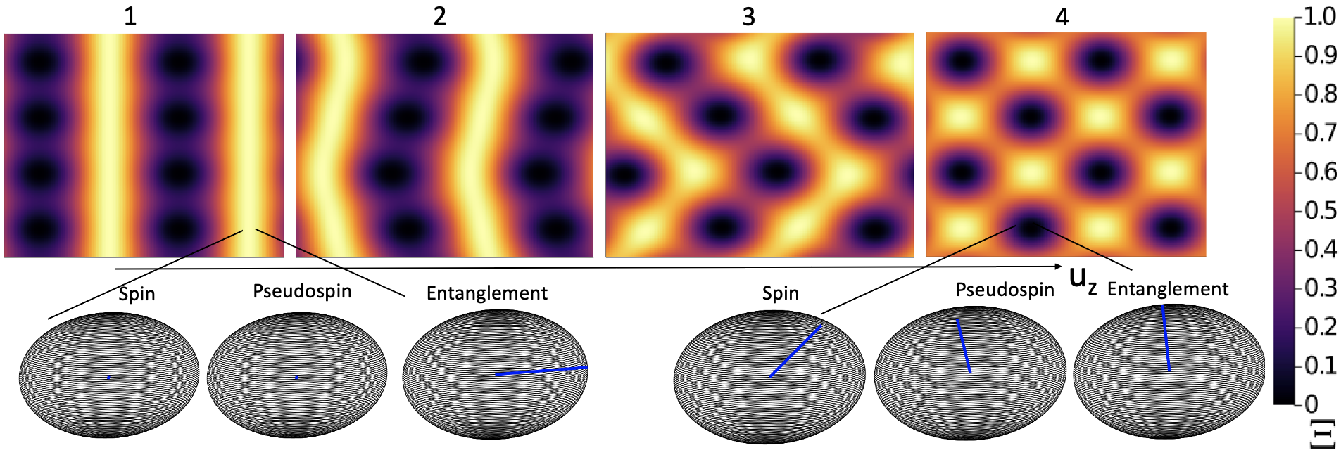
Figure 1: Entanglement patterns of the various entanglement ordered phases of multi-component ($\mathbb{C}P(3)$) textured crystals obtained on increasing the easy-axis anisotropy coupling constant ($u_{z}$ in Eq.(2)). Top row: From left to right we see first, the formation of continuous 1D straight lines of maximal entanglement $\Xi=1$, along the $y-$axis which have a discrete periodicity along $x$ - the entanglement smectic (1). Second, these straight lines start to modulate and form wavy patterns with modulated entanglement, which break the continuous translation symmetry of the smectic lines, while still maintaining a rotationally asymmetric and unidirectional nature - the entanglement stripe (3). As $u_{z}$ gets closer to $u_{p}$, $C_{4}$ symmetry is restored as in 4. Importantly, all above patterns have the same underlying $C_{4}$ symmetric charge density shown in Fig. 2 - it is the entanglement profile which breaks $C_{4}$ down to $C_{2}$. See Fig. 3a, to see $(u_{z},u_{p})$ values of 1-4. Bottom row: Bloch sphere representation of the local spin, pseudospin and entanglement vector for maximally (left) and minimally (right) entangled regions.

Model

For any quantum Hall ferromagnet, one can write the total energy for a 4-component spinor $\psi$ in an effective continuous theory as Sondhi et al. (1993); Moon et al. (1995)

$$E(\mathbf{\psi})=J\int d^{2}\textbf{r}\bigg{[}\dfrac{(\nabla\psi,\nabla\psi)}{(\psi,\psi)}-\dfrac{(\nabla\psi,\psi)(\psi,\nabla\psi)}{(\psi,\psi)}\bigg{]}+\\ g\int V(\mathbf{r}-\mathbf{r^{\prime}})Q(\textbf{r})Q(\textbf{r'})d^{2}\textbf{r}\>d^{2}\textbf{r'}+\int E_{A}(\mathbf{r})d^{2}\mathbf{r}$$ (1)

where $J$ and $g$ are coupling constants for the exchange and topological charge terms, $(a,b)\equiv\sum_{n=1}^{4}a^{*}_{n}b_{n}$, $V(\bf{r}-\bf{r}^{\prime})$ is the two body Coulomb potential (which we replace with a delta function term for analytical convenience in this work - see Methods) and $E_{A}$ is the anisotropy energy functional which breaks the approximate $SU(4)$ symmetry of the Coulomb interaction. We use the energy functional given in Kharitonov (2012); Lian et al. (2016) for anisotropies relevant to monolayer graphene, where pseudospin is the valley degree of freedom.

$$E_{A}(\ket{\psi(\mathbf{r})})=A\frac{\Delta_{Z}}{2}(u_{p}(M_{Px}^{2}+M_{Py}^{2})+u_{z}M_{Pz}^{2}-M_{Sz})$$ (2)

where $\Delta_{Z}\geq 0$ is proportional to the applied magnetic field, $u_{p}$ and $u_{z}$ characterize the pseudospin anisotropies which can be generated by short range interactions or lattice deformations due to phonon couplings and $A$ is a dimensionless constant.

To develop an analytical parameterization for skyrmion crystals for the above general energy functional, one must first consider an ansatz for the minimal energy configurations which imposes the constraint that the wavefunctions must be holomorphic. A natural choice of almost periodic holomorphic functions is the set of theta functions. The theta functions in our ansatz are

$$\theta_{p}(z)=\sum_{n=-\infty}^{\infty}e^{-\pi bd\frac{d}{a}(n+p/d)^{2}+2\pi\frac{d}{a}(n+p/d)z}$$ (3)

where $z=x+iy$ and we have $d$ skyrmions in a $a\times b$ unit cell ($d=4$ and $a=b$ for this work) and $p\in(0,1,..,d-1)$ in accordance with the Riemann-Roch theorem Debarre (2005). Our ansatz is for the simple case of a square lattice, however, symmetry breaking features of the entanglement measure presented in this work carry over to other shapes.

Using this basis of theta functions we construct the holomorphic spinor $\ket{\psi(\mathbf{r})}=F\ket{\psi_{0}(\mathbf{r})}$, where $\ket{\psi_{0}(\mathbf{r})}=(\theta_{0},\theta_{1},\theta_{2},\theta_{3})^{T}$ and $F$ is a $4\times 4$ $SU(4)$ matrix. The topological charge density term (see Methods) endows a stiffness to the crystal, and it was shown that all possible unitary matrices $F$ give rise to degenerate minimal energy configurations for skyrmion crystals with $SU(4)$-symmetric interactions Kovrizhin et al. (2013).

However, the anisotropy term lifts this large degeneracy and selects a subset among the $SU(4)$ manifold of $F$ matrices. Our assumptions to allow for such an analytic skyrmion crystal ansatz imply that we are working in a regime with $J\gg g\gg\Delta_{z}$. To obtain a general $SU(4)$ matrix $F$, we develop a parametrization technique, inspired from random matrix theory Diaconis and Forrester (2017), in terms of Euler angles (see Methods). Obtaining $\ket{\psi(\bf{r})}$ then reduces to a minimization problem for every $(u_{p},u_{z})$.

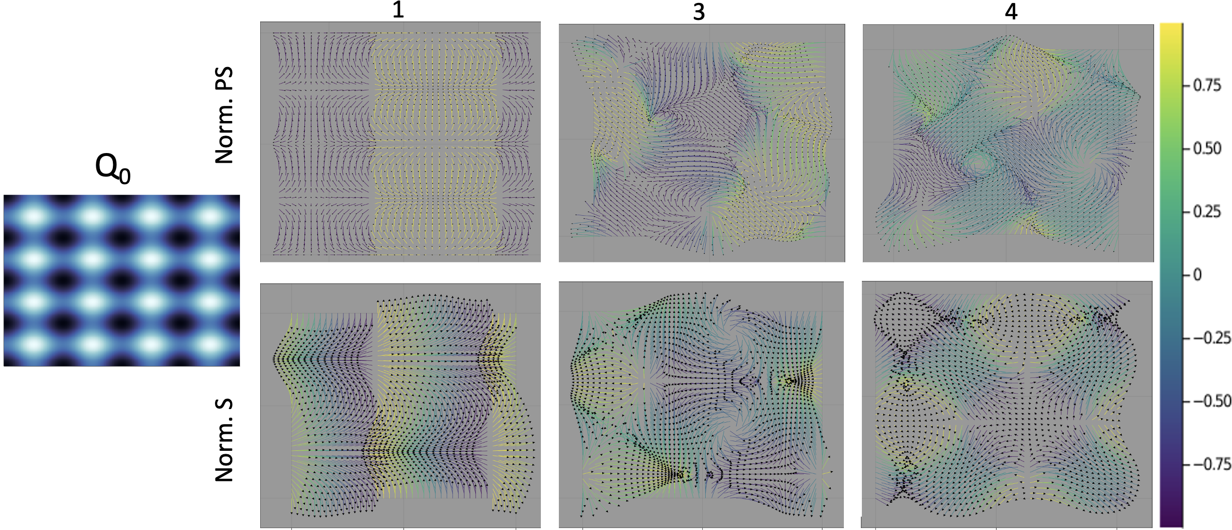
Figure 2: Underlying rotationally invariant $(C_{4})$ topological charge density (proportional to the charge density for quantum Hall skyrmion crystals) structure for the multi-component ($\mathbb{C}P(3)$) textured crystals and the different normalized spin and pseudospin ($\bm{M}_{P(S)}/\rm{cos}\alpha$) profiles obtained by increasing $u_{z}$. The length and direction of the arrows indicate the in-plane component and the color represents the out-of-plane component - violet for the south pole and bright yellow for the north (same direction as $B$-field). Note that there appear apparent discontinuities in the normalized spins, however these are not real discontinuities since these regions are maximally entangled regions where the actual spin/pseudospin components vanish. The numbers on top of the plots correspond to $u_{z}$ values in Fig. 3 a.

Schmidt decomposition and entanglement. Any normalized four-component complex ($\mathbb{C}P^{3}$) spinor can be written via a Schmidt decomposition in the form

$$\ket{\psi(\bf{r})}=\rm{cos}\frac{\alpha}{2}\ket{\Phi_{P}}\ket{\Phi_{S}}+e^{i\beta}\rm{sin}\frac{\alpha}{2}\ket{\Psi_{P}}\ket{\Psi_{S}}$$ (4)

where $\ket{\Phi_{S(P)}}$,$\ket{\Psi_{S(P)}}$ are orthogonal basis vectors belonging to the spin (pseudospin) subspace (see Douçot et al. (2008) for details). These basis vectors are parameterized by the usual spherical angles $(\theta_{S(P)},\phi_{S(P)})$. Along with $(\alpha,\beta)$, these angles define three Bloch vectors for spin, pseudospin and entanglement. The Bloch vectors defining the local spin and pseudospin magnetizations can be obtained from the spinor directly via

$$\mathbf{M}_{S}(\mathbf{r}) =\braket{\psi(\mathbf{r})}{1\otimes\mathbf{\sigma}}{\psi(\mathbf{r})}=\hat{n}(\theta_{S},\phi_{S})\rm{cos}(\alpha)$$ (5)

$$\mathbf{M}_{P}(\mathbf{r}) =\braket{\psi(\mathbf{r})}{\mathbf{\sigma}\otimes 1}{\psi(\mathbf{r})}=\hat{n}(\theta_{P},\phi_{P})\rm{cos}(\alpha)$$

where $\hat{n}$ is the unit vector on the sphere. In addition to these two, the entanglement Bloch vector is written as $\bm{m}_{E}=(\rm{sin}\alpha\,\rm{cos}\beta,\rm{sin}\alpha\,\rm{sin}\beta,\rm{cos}\alpha)$.

An immediate consequence of the entanglement between spin and pseudospin is the respective Bloch vectors shortening and hence exploring the interior of the sphere. Particularly drastic situations arise when at certain points in space there is maximal entanglement, i.e, the $\bm{M}_{P(S)}=\bm{0}$ (for $\alpha=\pi/2$). A convenient entanglement measure, in this context, is $\Xi=\rm{sin}^{2}\alpha$ Douçot et al. (2008).

Entanglement smectics and stripes. On analyzing the patterns of $\Xi(\bm{r})$ across the bulk, for certain cuts along $u_{p}-u_{z}$ parameter space we find phases with anisotropic profiles of spin-pseudospin entanglement. In these phases, the spatial profile of maximally entangled regions spontaneously breaks the four-fold ($C_{4}$) rotational symmetry of the underlying charge density of the crystal (Fig. 2), down to a two-fold one ($C_{2}$).

We identify two such entanglement orders - the entanglement smectic and entanglement stripe. In the former, maximally entangled regions ($\Xi=1$) form equidistant parallel lines as in Fig. 1-1, whereas in latter, the continuous translational symmetry (along $y$) of the maximally entangled regions is absent but the entanglement profile still maintains a unidirectional, discrete rotational symmetry broken pattern as in Fig. 1-3, much like uni-directional density waves. The symmetry features of these entanglement ordered phases are similar to the electronic smectic/stripe phase, discussed in quantum Hall and high-$T_{c}$ literature Koulakov et al. (1996); Moessner and Chalker (1996); Fradkin and Kivelson (1999); Emery et al. (1999, 2000). However, unlike charge or spin stripes (smectics) phases, the entanglement ordered phases have a four-fold symmetric charge density.

Such entanglement orders arise due to competition between different anisotropy terms given in eq. (2) in the presence of a dominant Coulomb interaction. Conventionally, the presence of these anisotropies would orient the spin and pseudospin vectors either in-plane or out-of-plane. However, in the $J\gg g\gg\Delta_{z}$ regime, the dominant Coulomb term imposes a topological charge density profile, such as the square lattice profile in Fig. 2 captured by our ansatz in eq. (3). As a consequence, we obtain a constrained optimization problem where the spins (pseudospins) cannot be all in-plane or out-of-plane and no single term in eq. (2) can be maximally satisfied. A compromise is allowed by spin-pseudospin entanglement which shortens the spin(pseudospin) vectors, and thereby reduces the energy loss from pseudospin terms in eq. (2). Such a reduction comes at a cost via a smaller gain from the Zeeman term which favours a larger spin magnitude.

Such an optimization problem induces the following features: First, there is no reduced $SU(2)$ description of these orders in terms of a collection of spin/pseudospin or even entanglement skyrmions Douçot et al. (2008); Lian et al. (2016), since the topological charge density constraint induces textures in all channels. Spin-pseudospin entanglement is maximal in regions which cost the most energy for a certain $(u_{p},u_{z})$. Second, the presence of a crystal adds the additional richness of packing of such non-uniform entanglement regions, especially for regions of maximal entanglement. These regions correspond to points at which the entanglement Bloch vector lies on the equator, which in turn corresponds to lines in real space (see Fig. 1). Hence, the problem becomes one of the optimal arrangement of such lines, inspiring connections with liquid crystals.

When $0<u_{z}<u_{p}/2$, the maximal energy cost comes from the in-plane pseudospin component. Due to the fixed topological charge constraint all pseudospins cannot be put out-of-plane. Hence, entanglement is energetically favoured in regions with maximal in-plane pseudospin, as it reduces the associated anisotropy cost. As a consequence, we see in Fig. 3, the entanglement stays constant till $u_{z}\sim u_{p}/2$, and the net out-of-plane pseudospin is much higher than that in-plane. Further, as we see from the spin profile, since $u_{p}>\Delta_{z}$ maximally entangled columns include spins pointing in opposite directions since the system compromises its gain from the zeeman term to prioritize reducing the in-plane pseudospin anisotropic cost (see Fig. 1-1 and Fig. 2). To maximize the area covered by the lines of maximal entanglement (by avoiding intersections) while respecting the symmetries imposed by the dominant Coulomb interaction which imposes square lattice charge density, the lines must be parallel. The system spontaneously chooses one of the two axes to align these lines with, thereby breaking the four-fold ($C_{4}$) symmetry down to two-fold ($C_{2}$).

On increasing $u_{z}$ beyond $u_{p}/2$, the anisotropy costs increase and so does the entanglement (see Fig. 3) since the easy-axis anisotropic cost becomes comparable to the easy-plane cost. Moreover, the distribution of maximally entangled regions changes as $u_{z}$ approaches $u_{p}$, resulting in transitions between different entanglement orders. Due to the competition between minimizing easy-axis and easy-plane costs, the entanglement spreads out spatially and the uniformity along one-dimensional smectics breaks up into a more general stripe order (see 1-3). Eventually when $u_{z}\sim u_{p}>\Delta_{z}$, the system restores four-fold rotational ($C_{4}$) symmetry (see 1-4). In the $u_{z}>u_{p}>\Delta_{z}$ regime, the pseudospin is mostly in-plane (see Fig. 2-4 and Fig. 3), and in regions where the topological charge density forces it to go out of plane, such as the core of the topological defects, the system maximally entangles, as seen in Fig. 2-4.

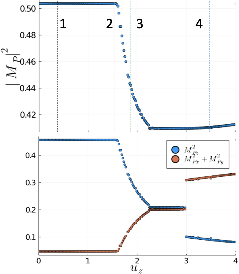
Figure 3: Entanglement order transitions on increasing easy-axis pseudospin anisotropy for $u_{p}=3\Delta_{z}$. (Top) Total pseudospin magnitude, the different numbered dash lines correspond to the respective profiles in Figs. 1 and 2. A continuous transition at $u_{z}=u_{p}/2$, from the entanglement smectic to the more general uni-directionally ordered entanglement stripe. Finally, there is another continuous transition corresponding to the restoration of four-fold rotational symmetry. See text for comments on transition at $u_{p}=u_{z}$. (Bottom) Out-of-plane and in-plane component of the pseudospin, as a function of easy-axis anisotropy.

Entanglement order transitions. As a consequence of such delicate competition we have two continuous entanglement order transitions. To study the nature of these transitions, we plot the average pseudospin magnitude and the out-of-plane component summed over all sites in Fig. 3. First there is a continuous transition at $u_{z}=u_{p}/2$ which corresponds to the deviation of maximally entangled regions from straight lines into wavy lines and modulated entanglement along those lines, thereby breaking the continuous translational symmetry along those lines. An appropriate order parameter for such a transition would be the amplitude of the periodic undulation of these lines along the transverse ($x$) direction. This corresponds to the entanglement smectic to entanglement stripe transition.

Next, there is another continuous transition corresponding to the restoration of $C_{4}$ symmetry. Such a transition occurs via melting of the entanglement stripe. Finally as we see from the jump in the in and out-of-plane components in Fig. 3b, there is another transition at $u_{p}=u_{z}$, however, there is no change in the symmetries of the entanglement structure across this transition.

Riemann-Goldstone Landau level structure and magnon transport signatures. In previous work, we showed that in the case where $J$ is the only non-zero energy scale, we get a series of effective Landau levels with the lowest Landau level being a flat band pinned to zero energy due to holomorphic constraints - the Riemann-Goldstone Landau level Chakraborty et al. (2023). For $g\neq 0$, the three Goldstone modes for the isotropic $SU(2)$ case would acquire a finite dispersion. In this work, for the $SU(4)$ case, we demonstrate the existence of 15 Goldstone modes and a single phonon mode in the Riemann-Goldstone Landau level based on counting independent small deformations in the zero momentum sector (see Methods). Moreover, using the axial gauge and a real-space discretization scheme (see Methods), we obtain their dispersion.

The anisotropy terms break the approximate $SU(4)$ symmetry and hence gap out 13 of the 15 type-preserving Goldstone modes. However, in addition to the phonon (only gapless in the continuum), there are remnant $U(1)_{P}$ and $U(1)_{S}$ symmetries which result in two gapless modes corresponding to a rotation about the $z-$axis of both spin and pseudospin. For $SU(4)$ ferromagnets, ref. Lian and Goerbig (2017) noted the presence of an extra $U(1)_{E}$ symmetry corresponding to the angle $\beta$ in the entanglement Bloch sphere. However, we do not get an additional gapless Goldstone branch for the skyrmion crystals considered here, because the $U(1)_{E}$ action involves non-linear transformations on the $\mathbb{C}P(3)$ manifold. As a result, the $U(1)_{E}$ action does not preserve the holomorphic nature of the texture, even for a uniform infinitesimal deformation.

A salient feature here, due to the highly anisotropic nature of the entanglement profile in the various phases, is the considerable anisotropy in the dispersion relation. One particularly notable case is that for the entanglement smectic. The group velocities for the two Goldstone modes of the entanglement smectic are heavily suppressed along one axis ($q_{x}$) of the Brillouin zone as compared to the other ($q_{y}$) (see Fig. 4). This suppression results in striking experimental consequences for magnon transport in quantum Hall heterojunction experiments.

Magnon transport in quantum Hall heterojunctions for graphene has emerged as a promising platform to detect the underlying spin structure of the quantum Hall phase diagram Wei et al. (2018); Zhou et al. (2020, 2022, 2021); Assouline et al. (2021). An intriguing question arising from our work is if magnon transmission can diagnose the entanglement structure. Say for example, we have the entangled smectic with uniform columns across which the spin vanishes (due to maximal entanglement). Such a configuration will not allow any low energy spin-wave approaching at normal incidence to pass through as the columns will act as a blockade, as seen from the extremely flat dispersions of the gapless modes along $q_{x}$ in Fig. 4. Hence, there will be almost full reflection of any such incoming magnon except perhaps at very special energies. Moreover, due to the strong anisotropy, there will be a strong dependence of the transmission on the incidence angle of the magnon. Such a drastic impedance mismatch is a unique consequence of such entanglement smectics, absent from any other kind of electronic order.

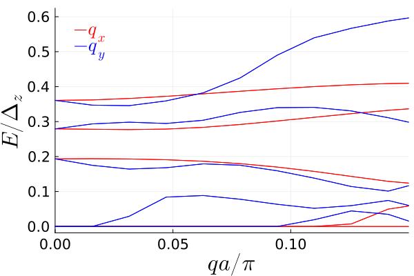
Figure 4: Lowest five modes' anisotropic dispersion of the entanglement smectic. Red (Blue) lines indicate dispersion along x (y) axis of first Brillouin zone. For weak values of $g$ ($g=J/20$, $u_{p}=3\Delta_{z}$ and $u_{z}=\Delta_{z}/10$ here), the two gapless modes remain relatively flat along $q_{x}$ whereas they become dispersive along $q_{y}$. For higher values of $g$ the two modes will eventually acquire a dispersion for both directions, however, the dispersion along $q_{x}$ will be strongly suppressed.

Discussion

In this work we have introduced the notion of anisotropic entanglement ordered phases which spontaneously break the discrete rotational symmetry of the charge density of the underlying crystal- the entanglement smectic and the entanglement stripe. We have also shown that these phases are associated with corresponding continuous entanglement order transitions. Finally, we have highlighted salient experimentally observable features of such entanglement orders in ongoing magnon transport experiments.

Besides transport, each of these anisotropic entanglement orders have a distinct spatial profile of the effective spin and pseudospin magnetization which could also be detected through imaging techniques like STM, which has achieved recent success in detecting symmetry broken phases in the lowest Landau level of graphene Feldman et al. (2016); Liu et al. (2022).

Our work, given the analogy with earlier seminal works in the quantum Hall and high-$T_{c}$ literature Koulakov et al. (1996); Moessner and Chalker (1996); Fradkin et al. (2010); Fradkin and Kivelson (1999); Emery et al. (2000, 1999); Kivelson et al. (2003); Millis and Norman (2007), raises the intriguing possibility of an entanglement nematic phase of matter, which would retain all translational symmetries and break only the rotational symmetry akin to the nematics found in liquid crystals. Following from this interesting questions on the melting of such stripe order and quantum criticality also arise.

Furthermore, several connections have been proposed between the physics of twisted bilayer graphene Cao et al. (2018a, b) and moiré systems in general, to multicomponent quantum Hall physics and skyrmions Bultinck et al. (2020); Khalaf et al. (2021); Khalaf and Vishwanath (2022). Such connections raise the exciting possibility of studying variations of such entanglement ordered phases between the different flavours in these systems, especially the dichalcogenides Seyler et al. (2019); Wang et al. (2020).

Methods

Discretizing $\mathbb{C}P(3)$ energy functional.

In this work we consider a delta function Coulomb potential and a reference topological charge density configuration generated by theta-functions, which is set to be the minimum of the energy functional (see discussion in Chakraborty et al. (2023) for experimental relevance).

A point in $\mathbb{C}P(N-1)$ is a line in $\mathbb{C}^{N}$ spanned by a non-zero $N$-component vector denoted by $\ket{\psi}$. As a preliminary step to discretize the energy functional let us specify the geodesics in $\mathbb{C}P(N-1)$ between $\mathbb{C}\ket{\psi_{1}}$ and $\mathbb{C}\ket{\psi_{2}}$ ($\mathbb{C}\ket{\psi}$ is the complex line in $\mathbb{C}^{N}$ space going through the vector $\psi$ and through the origin) with the $\braket{\psi}{\psi}=1$ constraint. We consider a map $\lambda\rightarrow\ket{\psi(\lambda)}$ such that $\ket{\psi(\lambda=0)}=\ket{\psi_{1}}$, $\ket{\psi(\lambda=1)}=\ket{\psi_{2}}$ and $\braket{\psi(\lambda)}{\psi(\lambda)}=1$. We may further choose phases of $\ket{\psi_{1}}$ and $\ket{\psi_{2}}$ such that $\braket{\psi_{1}}{\psi_{2}}\in\mathbb{R}$. We can define the angle $\theta\in[0,\pi/2]$ such that $\braket{\psi_{1}}{\psi_{2}}=\rm{cos}\,\theta$. The geodesic then corresponds to rotating $\ket{\psi_{1}}$ into $\ket{\psi_{2}}$ with constant angular velocity, which can be written as

$$\ket{\psi(\lambda)}=\dfrac{\rm{sin}(\theta(1-\lambda))\ket{\psi_{1}}+\rm{sin}(\theta\lambda)\ket{\psi_{2}}}{\rm{sin}\,\theta}$$ (6)

The geodesic length in $\mathbb{C}P(N-1)$ is simply $\theta$, which in the general case of $\braket{\psi_{1}}{\psi_{2}}\in\mathbb{C}$ is given by $\rm{cos}\,\theta=(\braket{\psi_{1}}{\psi_{2}}\braket{\psi_{2}}{\psi_{1}})/(\braket{\psi_{1}}{\psi_{1}}\braket{\psi_{2}}{\psi_{2}})^{1/2}$.

Say $\ket{\psi_{1}}$ and $\ket{\psi_{2}}$ correspond to the spinors on neighbouring sites, which implies that they differ by a small angle $\theta\approx 0$, we can write

$$\theta^{2}=1-\dfrac{\braket{\psi_{1}}{\psi_{2}}\braket{\psi_{2}}{\psi_{1}}}{\braket{\psi_{1}}{\psi_{1}}\braket{\psi_{2}}{\psi_{2}}}$$ (7)

which is gauge invariant. Therefore a natural discretization for the local exchange term can be written as

$$E_{\rm{exc}}=J\sum_{<i,j>}\bigg{(}1-\dfrac{\braket{\psi_{i}}{\psi_{j}}\braket{\psi_{j}}{\psi_{i}}}{\braket{\psi_{i}}{\psi_{i}}\braket{\psi_{j}}{\psi_{j}}}\bigg{)}$$ (8)

where the sum is over nearest neighbour pairs.

To discretize the topological charge density terms, one needs to consider 4 spinors associated with the sites of a plaquette in real space. The procedure to calculate this for the simpler $SU(2)$ skyrmion crystal using local spin vectors was introduced in ref.Chakraborty et al. (2023). The basic idea is to consider the nearest neighbours pairwise and calculate the topological charge between two nearby geodesics. We show here how to do this for the $\mathbb{C}P(3)$ manifold.

Consider a closed path $\gamma$ in $\mathbb{C}P(N-1)$ parametrized by $t\in[0,1]$. The topological charge associated to this path has the general form $\oint\mathcal{A}$, where $\mathcal{A}$ is a 1-form on $\mathbb{C}P(N-1)$ whose curl is equal to the canonical symplectic two form on $\mathbb{C}P(N-1)$ associated to the Fubini-Study metric. A convenient way to evaluate $\oint\mathcal{A}$ is to take a map $t\rightarrow\ket{\psi(t)}\in\mathbb{C}^{N}-{0}$ such that $\mathbb{C}\ket{\psi(t)}=\gamma(t)$ at all $t$. Such a procedure is called lifting the path. It is essential that this lifted path be closed as well, i.e $\ket{\psi(0)}=\ket{\psi(1)}$, in order to get an expression which is independent of the choice of such a path. Then we get

$$Q_{\gamma}=\frac{1}{2i}\int_{0}^{1}\dfrac{\braket{\psi}{\dot{\psi}}-\braket{\dot{\psi}}{\psi}}{\braket{\psi}{\psi}}dt$$ (9)

Let us now consider a geodesic quadrangle on $\mathbb{C}P(N-1)$ where $\mathbb{C}\ket{\psi_{j}^{\prime}}$ is very close to $\mathbb{C}\ket{\psi_{j}}$ ($j=0,1$), so we may set $\ket{\psi_{j}^{\prime}}=\ket{\psi_{j}}+\ket{\chi_{j}}$. If we consider the quadrangle comprising the two initial ($\psi_{0},\psi_{1}$) and two final ($\psi^{\prime}_{0},\psi^{\prime}_{1}$) points, we can write

$$\begin{split}Q_{01}&=\rm{arg}\bigg{(}\dfrac{\braket{\psi_{0}}{\psi^{\prime}_{0}}}{\braket{\psi_{0}}{\psi_{0}}}\bigg{)}+\rm{arg}\bigg{(}\dfrac{\braket{\psi_{0}^{\prime}}{\psi_{1}^{\prime}}}{\braket{\psi_{0}}{\psi_{1}}}\bigg{)}+\rm{arg}\bigg{(}\dfrac{\braket{\psi_{1}^{\prime}}{\psi_{1}}}{\braket{\psi_{1}}{\psi_{1}}}\bigg{)}\\ &=\frac{1}{2i}\bigg{(}\dfrac{\braket{\psi_{0}}{\chi_{0}}-\braket{\chi_{0}}{\psi_{0}}}{\braket{\psi_{0}}{\psi_{0}}}+\dfrac{\braket{\psi_{0}}{\chi_{1}}+\braket{\chi_{0}}{\psi_{1}}}{\braket{\psi_{0}}{\psi_{1}}}-\\ &\quad\dfrac{\braket{\chi_{1}}{\psi_{0}}+\braket{\psi_{1}}{\chi_{0}}}{\braket{\psi_{1}}{\psi_{0}}}+\dfrac{\braket{\chi_{1}}{\psi_{1}}-\braket{\psi_{1}}{\chi_{1}}}{\braket{\psi_{1}}{\psi_{1}}}\bigg{)}\end{split}$$ (10)

The total contribution from the plaquette $0123$ is then given by $Q_{0123}=Q_{01}+Q_{12}+Q_{23}+Q_{30}$. Finally, the contribution to the topological charge density term for the site $0$ is given by $\sum_{0\in\square}Q_{\square}^{2}$.

Euler angle parameterization of a general SU(4) matrix. Let $(e_{1},e_{2},...,e_{N})$ be an orthonormal basis in $\mathbb{C}^{N}$. The idea is to use a recursive procedure in order to parametrize all matrices in $SU(N)$ corresponding to isometries $f:\mathbb{C}^{N}\rightarrow\mathbb{C}^{N}$. Suppose that we know how to find a rotation $g_{1}\in SU(N)$ such that $g_{1}(e_{1})=f(e_{1})$, which amounts to saying that the first columns of the matrices representing $f$ and $g_{1}$ are identical. The explicit parametrization of such a $g_{1}$ will be given below. Let us introduce a rotation $f_{2}$ given by $f=g_{1}f_{2}$, then $f_{2}(e_{1})=e_{1}$. The matrix representing $f_{2}$ has $1$ in the top left and then a diagonal block $M_{2}\in SU(N-1)$. We apply the same procedure to $M_{2}$, i.e we search for $g_{2}\in SU(N-1)$ such that $g_{2}(e_{1})=f_{2}(e_{1})=e_{1}$ and $g_{2}(e_{2})=f_{2}(e_{2})\in\rm{Vect}(e_{2},e_{3},...,e_{N})$. Then $f_{2}=g_{2}f_{3}$ with $f_{3}(e_{1})=e_{1}$ and $f_{3}(e_{2})=e_{2}$. Now $f_{3}$ is a matrix with two diagonal blocks, the identity matrix $\mathbb{1}_{2}$ and $M_{3}\in SU(N-2)$. We keep applying this procedure to the nested sequence of groups $SU(N)\supset SU(N-1)\supset...\supset SU(2)$. In this decreasing sequence of groups, $SU(N-p)$ is understood as the subgroup of $SU(N)$ of rotations which leave $e_{1},...,e_{p}$ invariant. In the end we get

$$f=g_{1}g_{2}\dots g_{N-1}$$ (11)

It remains then to find a convenient parametrization for the $g_{1}$ rotation. We know that $g(e_{1})\in\rm{Vect}({e_{1},..e_{N}})$ is given (where Vect$(e_{1},\dots,e_{i})$ implies that the vector has $i$ non-zero components). The idea is to go from $e_{1}$ to $g(e_{1})$ step by step, switching on sequentially the non-zero component of $g(e_{1})$ starting from $x_{2}$, then $x_{3}$ and so on up to $x_{N}$. For this, we write $f(e_{1})=h_{N}h_{N-1}\dots h_{2}(e_{1})$ with

$$\begin{split}h_{2}(e_{1})&\equiv v_{2}\in\rm{Vect}(e_{1},e_{2})\\ h_{3}(v_{2})&\equiv v_{3}\in\rm{Vect}(e_{1},e_{2},e_{3})\\ &.\\ &.\\ h_{N}(v_{N-1})&\equiv g(e_{1})\in\rm{Vect}(e_{1},e_{2},...,e_{N})\end{split}$$ (12)

Let us define $R_{j}(\theta_{j},\phi_{j},\psi_{j})\in SU(N)$ as the rotation such that

$$\begin{split}R_{j}(\theta_{j},\phi_{j},\psi_{j})(e_{k})&=e_{k};k\notin{j-1,j}\\ R_{j}(\theta_{j},\phi_{j},\psi_{j})(e_{j-1})&=\rm{cos}(\theta_{j})e^{i\psi_{j}}e_{j-1}+\rm{sin}(\theta_{j})e^{i\phi_{j}}e_{j}\\ R_{j}(\theta_{j},\phi_{j},\psi_{j})(e_{j})&=-\rm{sin}(\theta_{j})e^{-i\phi_{j}}e_{j-1}+\rm{cos}(\theta_{j})e^{-i\psi_{j}}e_{j}\\ \end{split}$$ (13)

Using such a parametrization one can show that Eq. (12) is always satisfied with rotation matrices chosen as $h_{j}=R_{j}(\theta_{j},\phi_{j},\psi_{j})$. We start from $h_{N}$, and we write $f(e_{1})=g(e_{1})=x_{1}e_{1}+\dots+x_{N}e_{N}$ ($\sum_{i}|x_{i}|^{2}=1$). We wish to find $v_{N-1}=y_{1}e_{1}+\dots+y_{N-1}e_{N-1}$ ($\sum_{i}|y_{i}|^{2}=1$ and we can always choose $y_{N-1}$ to be a non-negative real number) and $\theta_{N}\in[0,\pi/2]$, $\phi_{N}\in[0,2\pi]$, $\psi_{N}\in[0,2\pi]$ such that $R_{N}(\theta_{N},\phi_{N},\psi_{N})(v_{N-1})=g(e_{1})$. This condition implies that $y_{k}=x_{k}$ for $k=(1,...,N-2)$ and

$$\begin{split}y_{N-1}\cos(\theta_{N})e^{i\psi_{N}}&=x_{N-1}\\ y_{N-1}\sin(\theta_{N})e^{i\phi_{N}}&=x_{N}\end{split}$$ (14)

One can write the polar decomposition of the R.H.S of the above equation to obtain the three Euler angles. Once $v_{N-1}\in\rm{Vect}(e_{1},...,e_{N-1})$ is determined we set to find $v_{N-2}\in\rm{Vect}(e_{1},..,e_{N-2})$ and $[\theta_{N-1},\phi_{N-1},\psi_{N-1}]$ such that $R_{N-1}(\theta_{N-1},\phi_{N-1},\psi_{N-1})(v_{N-2})=v_{N-1}$. One can solve this using the similar procedure which resulted in Eq. (14). Because $y_{N-1}$ is real and non-negative, we see that if we take the component of $v_{N-2}$ along $e_{N-2}$ to be also real and non-negative, then $\phi_{N-1}=0$. Continuing this process recursively one determines all the Euler angles, from $N-1$ to $2$. Therefore we can write

$$g_{1}=R_{N}(\theta_{N})R_{N-1}(\theta_{N-1})\dots R_{2}(\theta_{2})$$ (15)

where we have hidden the dependence on the other $\phi$ and $\psi$ angles for notational convenience. As we saw earlier, only $\phi_{N}\neq 0$, so $g_{1}$ in the above equation depends only on $2N-1$ real parameters, as it should because $f(e_{1})$ belongs to the unit sphere in $\mathbb{C}^{N}$, whose dimension is precisely $2N-1$. Since we have to also decompose $g_{2},\dots,g_{N-1}$ in a similar fashion, we have to introduce $2N-1+\dots+5+3=N^{2}-1$ Euler angles for an arbitrary matrix in $SU(N)$.

One can write these product decompositions as

$$\begin{split}g_{1}&=R_{N}(\theta_{1,N})R_{N-1}(\theta_{1,N-1})\dots R_{2}(\theta_{1,2})\\ g_{2}&=R_{N}(\theta_{2,N})R_{N-1}(\theta_{2,N-1})\dots R_{3}(\theta_{2,3})\\ &.\\ &.\\ g_{j}&=R_{N}(\theta_{j,N})R_{N-1}(\theta_{j,N-1})\dots R_{j+1}(\theta_{j,j+1})\\ &.\\ &.\\ g_{N-1}&=R_{N}(\theta_{N-1,N})\end{split}$$ (16)

Using these results for eq. (11) we obtain the matrix $f$.

$\mathbb{C}P(3)$ equations of motion. The kinetic term of the Lagrangian gives the Berry phase and is written as:

$$\mathcal{L}_{k}=\frac{1}{2i}\dfrac{\braket{\psi}{\dot{\psi}}-\braket{\dot{\psi}}{{\psi}}}{\braket{\psi}{\psi}}$$ (17)

Under a gauge transformation $\ket{\psi(t)}=f(t)e^{i\alpha(t)}\ket{\chi(t)}$, which gives

$$\mathcal{L}_{k}(\psi,\dot{\psi})=\mathcal{L}_{k}(\chi,\dot{\chi})+\dot{\alpha}$$ (18)

So provided $\alpha(0)=\alpha(1)$, we have $\int_{0}^{1}\mathcal{L}_{k}(\psi,\dot{\psi})dt=\int_{0}^{1}\mathcal{L}_{k}(\chi,\dot{\chi})dt$ (this in particular the case if we keep the end points of the path fixed, i.e $\alpha(0)=\alpha(1)=0$). The potential term $\mathcal{L}_{p}(\psi^{*},\psi)$ is invariant under gauge transformations $\psi_{a}\rightarrow\epsilon\psi_{a}$, with ($1\leq a\leq N$) and $\epsilon$ an arbitrary complex number. From this we get

$$\sum_{a=1}^{N}\frac{\partial\mathcal{L}_{p}}{\partial\psi_{a}}(\psi^{*},\psi)\psi_{a}=\sum_{a=1}^{N}\frac{\partial\mathcal{L}_{p}}{\partial\psi^{*}_{a}}(\psi^{*},\psi)\psi^{*}_{a}=0$$ (19)

The Euler-Lagrange equations of motion read

$$i\big{(}\dfrac{\dot{\psi}_{a}}{\braket{\psi}{\psi}}-\dfrac{\braket{\psi}{\dot{\psi}}}{\braket{\psi}{\psi}^{2}}\psi_{a}\big{)}=\dfrac{\partial\mathcal{L}_{p}}{\partial\psi_{a}^{*}}$$ (20)

Multiplying the L.H.S by $\psi_{a}^{*}$ and summing over $a$ gives 0, which is compatible with the gauge invariance of the potential term as expressed in Eq. (19). Let us assign $s_{a}\equiv-i(\partial\mathcal{L}_{p}/\partial\psi_{a}^{*})$, the above equation can then be written in terms of $s_{a}$ and it determines $\ket{\dot{\psi}}$ up to a vector proportional to $\ket{\psi}$. We can write

$$\ket{\dot{\psi}}=\braket{\psi}{\psi}\ket{s}+b\ket{\psi}$$ (21)

where $b$ is an arbitrary complex number. We can eliminate this redundancy in the choice of $b$ using the axial gauge. We wish to impose

$$\braket{g}{\dot{\psi}}=0$$ (22)

where $g$ is a given time-independent $N$-component complex vector. Most often $g$ will be chosen of the form $g_{a}=\delta_{ai}$ with fixed $i$ (at a given site). Imposing the above determines $b$ provided that $\braket{g}{\psi}\neq 0$. Then

$$b =-\braket{\psi}{\psi}\dfrac{\braket{g}{s}}{\braket{g}{\psi}}$$ (23)

$$\ket{\dot{\psi}} =\braket{\psi}{\psi}\left(\ket{s}-\dfrac{\braket{g}{s}}{\braket{g}{\psi}}\ket{\psi}\right)$$ (24)

To obtain the linearized equations of motion we start from of variational ground-state $\ket{\psi}$ and look for time dependent solutions of the form $\ket{\psi}+\ket{\chi(t)}$ with $\ket{\chi(t)}$ small. To first order in $\chi$ we get

$$\dfrac{\ket{\dot{\chi}}}{\braket{\psi}{\psi}} -\dfrac{\braket{\psi}{\dot{\psi}}}{\braket{\psi}{\psi}^{2}}\ket{\psi}=\ket{s}$$ (25)

$$s_{a} =-i\sum_{b=1}^{N}\big{(}\dfrac{\partial^{2}\mathcal{L}_{p}}{\partial\chi_{a}^{*}\partial\chi_{b}}\chi_{b}+\dfrac{\partial^{2}\mathcal{L}_{p}}{\partial\chi_{a}^{*}\partial\chi_{b}^{*}}\chi^{*}_{b}\big{)}$$ (26)

The above equation however does not have a solution when $\ket{\psi}$ is not an exact energy extremum, as it is the case in our variational procedure, where the energy functional is minimized over the global choice of an $SU(4)$ matrix $F$. To rectify this we can project $\ket{s}$ into the subspace orthogonal to $\ket{\psi}$. This gives us the following form for the equations of motion

$$\ket{\dot{\chi}}=\braket{\psi}{\psi}\big{(}\ket{s}-\dfrac{\braket{g}{s}}{\braket{g}{\psi}}\ket{\psi}\big{)}$$ (27)

However, to ensure discrete translational invariance one has to make a small modification and replace $\ket{\chi}$ by $\ket{w}=\langle g|\psi\rangle^{-1}\ket{\chi}$. The final equations of motion are

$$\ket{\dot{w}}=\dfrac{\braket{\psi}{\psi}}{\langle g|\psi_{0}\rangle}\left(\ket{s}-\dfrac{\braket{g}{s}}{\braket{g}{\psi}}\ket{\psi}\right)$$ (28)

where $\ket{s}$ in the R.H.S is now expressed as a function of $\ket{w}$.

Goldstone mode counting. In this section we present a mathematically rigorous argument for the existence of 15 type-preserving Goldstone modes (of which 13 are gapped out in presence of anisotropies) in the Riemann-Goldstone Landau level as well as a phonon, for the model that we considered above.

Let us examine the structure of small deformations at $\bm{q}=0$. Let us consider the texture described by the map $z\rightarrow(\theta_{0}(z),\theta_{1}(z),\dots,\theta_{N-1}(z))\equiv\ket{\psi(z)}$. We have two kinds of deformations in the $\bm{q}=0$ sector around such optimal crystals.

a) Type-preserving deformations: We deform $\ket{\psi(z)}$ into $\ket{\psi(z)}$ + $\ket{\chi(z)}$, with $\ket{\chi(z)}$ of the form

$$\chi_{a}(z)=\sum_{b=0}^{N-1}M_{ab}\theta_{b}(z)$$ (29)

where $M$ is a $N\times N$ matrix. We call such deformations type-preserving, because they don't require to modify the theta function basis used to describe the deformed texture. This gives us a continuous family of $q=0$ deformations with $2(N^{2}-1)$ real parameters, after excluding gauge transformations corresponding to $M$ matrices proportional to the identity.

b) Phonon deformations: These are of the form

$$\chi_{a}(z)=u\psi^{\prime}_{a}(z);\;u\in\mathbb{C}$$ (30)

where $\psi^{\prime}_{a}(z)=\partial\psi_{a}/\partial z$. Such deformations are not type-preserving since the derivative of a theta function doesn't transform under lattice translations as a theta function, hence these continuous translations cannot be accounted for without changing the underlying theta function basis. It is well known in the mathematics literature that line bundles (and their associated theta functions) of fixed degree $N$ on a torus have exactly one free complex deformation parameter, which can be visualized as the center of mass position of the set of zeros of theta functions inside a given unit cell. So, this suggests that phonon deformations exhaust all type deforming deformations which preserve the discrete lattice periodicity of the texture.

A general $q=0$ deformation may be written as

$$\chi_{a}(z)=\sum_{b=0}^{N-1}M_{ab}\theta_{b}(z)+u\psi^{\prime}_{a}(z)$$ (31)

with $\rm{trace}(M)=0$. Such deformations involve $2N^{2}$ real parameters.

$SU(N)$ symmetry generates 15 independent flat directions, i.e, small deformations that do not change the energy. We show below that these 15 directions are mutually orthogonal for the symplectic form that generates the linearized equations of motion. As a result we'll see that the 15 flat directions give 15 zero eigenvectors and 15 two-dimensional Jordan blocks. Recall that a 2D Jordan block arises from linearizing the free particle motion, generated by $H=p^{2}/2$, in the vicinity of any equilibrium point $(p,q)=(0,q_{0})$ in phase-space.

Symplectic form for small deformations in the $q=0$ sector: Take $\chi_{a}^{(1)}(z)$ and $\chi_{a}^{(2)}(z)$ to be two small deformations around the optimal Skyrmion crystal described by the holomorphic map $z\rightarrow\ket{\psi(z)}$. We define

$$\Omega\big{[}\chi^{(1)},\;\chi^{(2)}\big{]}\equiv i\int dxdy\bigg{[}\dfrac{\langle\chi_{2}|\;(\mathbb{1}-P_{\psi})\;|\chi_{1}\rangle}{\langle\psi|\psi\rangle}-\\ \dfrac{\langle\chi_{1}|\;(\mathbb{1}-P_{\psi})\;|\chi_{2}\rangle}{\langle\psi|\psi\rangle}\bigg{]}$$ (32)

where $P_{\psi}=\ket{\psi(z)}\bra{\psi(z)}/\langle\psi(z)|\psi(z)\rangle$ and we have hidden the $z-$dependence for notational convenience. We use this symplectic form because equations of the motion have the generalized Hamiltonian form:

$$i\bigg{(}\dfrac{\dot{\psi}_{a}(\bm{r})}{\langle\psi(\bm{r})|\psi(\bm{r})\rangle}-\dfrac{\langle\psi(\bm{r})|\dot{\psi}(\bm{r})\rangle\psi_{a}(\bm{r})}{\langle\psi(\bm{r})|\psi(\bm{r})\rangle^{2}}\bigg{)}=\dfrac{\partial\mathbb{L}_{p}}{\partial\psi^{*}_{a}(\bm{r})}$$ (33)

where $\mathbb{L}_{p}$ is the potential energy functional, and one can obtain these equations by imposing that

$$\Omega\big{[}\dot{\psi},\chi]=\int d^{2}r\bigg{(}\dfrac{\partial\mathbb{L}_{p}}{\partial\psi^{*}_{a}(\bm{r})}\chi_{a}^{*}(\bm{r})+\dfrac{\partial\mathbb{L}_{p}}{\partial\psi_{a}(\bm{r})}\chi_{a}(\bm{r})\bigg{)}$$ (34)

for all possible small deformations $\chi_{a}(\bm{r})$, $1\leq a\leq N$. $\Omega[\chi^{(1)},\chi^{(2)}]$ takes real values, is antisymmetric in $\chi^{(1)},\chi^{(2)}$ and is $\mathbb{R}$-bilinear (but not $\mathbb{C}$-bilinear).

Main properties of $\Omega$ (in the $q=0$ subspace): Phonon deformations and type preserving ones are $\Omega$-orthogonal: To see this consider $\ket{\chi^{(1)}}=M\ket{\psi}$, with $M$ a constant $N\times N$ matrix and $\ket{\chi^{(2)}}=\ket{\psi^{\prime}}$. Now

$$\Omega\big{[}M\ket{\psi},\lambda\ket{\psi^{\prime}}\big{]}=i\int_{\rm{unit}\,\rm{cell}}\lambda^{*}\dfrac{\langle\psi^{\prime}|(\mathbb{1}-P_{\psi})M|\psi\rangle}{\langle\psi|\psi\rangle}-\\ \lambda\dfrac{\langle\psi|M^{\dagger}(\mathbb{1}-P_{\psi})|\psi^{\prime}\rangle}{\langle\psi|\psi\rangle}$$ (35)

where $\lambda\in\mathbb{C}$. Each of the two terms in the integrand is a derivative of a periodic function, so the integrand over a unit cell vanishes. For example, we have:

$$\dfrac{\partial}{\partial z}\bigg{(}\dfrac{\langle\psi|M^{\dagger}|\psi\rangle}{\langle\psi|\psi\rangle}\bigg{)}=\bigg{(}\dfrac{\langle\psi|M^{\dagger}(\mathbb{1}-P_{\psi})|\psi^{\prime}\rangle}{\langle\psi|\psi\rangle}\bigg{)}$$ (36)

The two phonon deformations are mutually conjugate: Consider $\ket{\chi^{(1)}}=w^{(1)}\ket{\psi^{\prime}(z)}$ and $\ket{\chi^{(2)}}=w^{(2)}\ket{\psi^{\prime}(z)}$

$$\Omega\big{(}\chi^{(1)},\chi^{(2)}\big{)}=i\int_{\rm{unit}\,\rm{cell}}\dfrac{\langle\psi^{\prime}|\mathbb{1}-P_{\psi}|\psi^{\prime}\rangle}{\langle\psi|\psi\rangle}(w_{1}w^{*}_{2}-w_{2}w^{*}_{1})$$ (37)

The integrand is equal to twice the topological charge density because $\ket{\psi}$ is holomorphic. This implies that

$$\Omega\big{(}\chi^{(1)},\chi^{(2)}\big{)}=4\pi iN(w_{1}w^{*}_{2}-w_{2}w^{*}_{1})$$ (38)

Let us now further investigate the symplectic form within this subspace of type-preserving deformations, i.e we take $\ket{\chi^{(1)}}=M_{1}\ket{\psi}$ and $\ket{\chi^{(2)}}=M_{2}\ket{\psi}$. We can then write

$$\Omega\big{[}M_{1}\ket{\psi},M_{2}\ket{\psi}\big{]}=i\int_{\rm{unit}\,\rm{cell}}\dfrac{\langle\psi|M_{2}^{\dagger}(\mathbb{1}-P_{\psi})M_{1}|\psi\rangle}{\langle\psi|\psi\rangle}-\\ \dfrac{\langle\psi|M_{1}^{\dagger}(\mathbb{1}-P_{\psi})M_{2}|\psi\rangle}{\langle\psi|\psi\rangle}$$ (39)

Furthermore, any matrix $M$ can be written as a sum of hermitian and anti-hermitian matrices. If $M_{1}$ and $M_{2}$ are both hermitian/non-hermitian, then the corresponding deformations are $\Omega-$orthogonal.

Matrices with antihermitian generators correspond to infinitesimal SU(N) transformations, they form a $N^{2}-1$ dimensional subspace over $\mathbb{R}$ playing the role of $q_{j}$ coordinates ($1\leq j\leq N^{2}-1$). We also get a complementary $N^{2}-1$ dimensional subspace, composed of the traceless hermitian deformations, playing the role of $p_{j}$ (conjugate) coordinates. This yields the $N^{2}-1$ Jordan blocks because invariance of the total energy under $q-$translations imposes that the Taylor expansion around an optimal crystal contain only $p_{i}p_{j}$ terms.

For phonon deformations $\ket{\chi}=\lambda\ket{\psi^{\prime}}$, we may write $\lambda=q_{0}+ip_{0}$ with $q_{0}$ and $p_{0}$ real and eq. (38) shows that (after a proper normalization) $q_{0}$ and $p_{0}$ can be taken as a pair of canonically conjugate coordinates. So phonon deformations (at $q=0$) give rise to a zero frequency oscillator, instead of a Jordan block.

In the presence of anisotropies described by eq. (2), the original $SU(4)$ symmetry is broken into the much smaller two-dimensional $U(1)_{P}\times U(1)_{S}$ subgroup, turning 13 among the previous 15 Jordan blocks into finite frequency oscillators. Moving away from the $q=0$ sector and considering small but finite $q$ values also transforms each remaining Jordan block and the phonon mode into an oscillator mode, whose frequency depends smoothly on $q$.

Acknowledgements: This work was in part supported by the Deutsche Forschungsgemeinschaft under grants SFB 1143 (project-id 247310070) and the cluster of excellence ct.qmat (EXC 2147, project-id 390858490). B. D. thanks MPIPKS for its generous hospitality during several extended visits, which were crucial for the realization of this project. This research was supported in part by grants NSF PHY-1748958 and PHY-2309135 to the Kavli Institute for Theoretical Physics (KITP).

References

- Anderson (2018) P. W. Anderson, Basic notions of condensed matter physics (CRC Press, 2018).
- Koulakov et al. (1996) A. A. Koulakov, M. M. Fogler, and B. I. Shklovskii, Phys. Rev. Lett. 76, 499 (1996).
- Moessner and Chalker (1996) R. Moessner and J. T. Chalker, Phys. Rev. B 54, 5006 (1996).
- Emery et al. (1999) V. Emery, S. Kivelson, and J. Tranquada, Proceedings of the National Academy of Sciences 96, 8814 (1999).
- Emery et al. (2000) V. J. Emery, E. Fradkin, S. A. Kivelson, and T. C. Lubensky, Phys. Rev. Lett. 85, 2160 (2000).
- Fradkin and Kivelson (1999) E. Fradkin and S. A. Kivelson, Phys. Rev. B 59, 8065 (1999).
- Lilly et al. (1999) M. P. Lilly, K. B. Cooper, J. P. Eisenstein, L. N. Pfeiffer, and K. W. West, Phys. Rev. Lett. 82, 394 (1999).
- Du et al. (1999) R. R. Du, D. C. Tsui, H. L. Stormer, L. N. Pfeiffer, K. W. Baldwin, and K. W. West, Solid State Communications 109, 389 (1999).
- Wu et al. (2011) T. Wu, H. Mayaffre, S. Krämer, M. Horvatić, C. Berthier, W. Hardy, R. Liang, D. Bonn, and M.-H. Julien, Nature 477, 191 (2011).
- Millis and Norman (2007) A. J. Millis and M. R. Norman, Phys. Rev. B 76, 220503 (2007).
- Fradkin et al. (2010) E. Fradkin, S. A. Kivelson, M. J. Lawler, J. P. Eisenstein, and A. P. Mackenzie, Annu. Rev. Condens. Matter Phys. 1, 153 (2010).
- Kivelson et al. (2003) S. A. Kivelson, I. P. Bindloss, E. Fradkin, V. Oganesyan, J. M. Tranquada, A. Kapitulnik, and C. Howald, Rev. Mod. Phys. 75, 1201 (2003).
- Nielsen and Chuang (2010) M. A. Nielsen and I. L. Chuang, Quantum computation and quantum information (Cambridge university press, 2010).
- Horodecki et al. (2009) R. Horodecki, P. Horodecki, M. Horodecki, and K. Horodecki, Reviews of modern physics 81, 865 (2009).
- (15) Spin-pseudospin coupling is different from spin-pseudospin entanglement. The former is a necessary but insufficient condition for the latter. In this case entanglement is defined as the "non-classical" correlations between the spin and pseudospin "qubits".
- Lian and Goerbig (2017) Y. Lian and M. O. Goerbig, Phys. Rev. B 95, 245428 (2017).
- Murthy et al. (2017) G. Murthy, E. Shimshoni, and H. A. Fertig, Phys. Rev. B 96, 245125 (2017).
- Stefanidis and Villadiego (2023) N. Stefanidis and I. S. Villadiego, arXiv:2309.07217 (2023).
- Tarnopolsky et al. (2019) G. Tarnopolsky, A. J. Kruchkov, and A. Vishwanath, Phys. Rev. Lett. 122, 106405 (2019).
- Bultinck et al. (2020) N. Bultinck, E. Khalaf, S. Liu, S. Chatterjee, A. Vishwanath, and M. P. Zaletel, Phys. Rev. X 10, 031034 (2020).
- Brey et al. (1995) L. Brey, H. A. Fertig, R. Côté, and A. H. MacDonald, Phys. Rev. Lett. 75, 2562 (1995).
- Sondhi et al. (1993) S. L. Sondhi, A. Karlhede, S. A. Kivelson, and E. H. Rezayi, Phys. Rev. B 47, 16419 (1993).
- Goerbig et al. (2006) M. O. Goerbig, R. Moessner, and B. Douçot, Physical Review B 74, 161407 (2006).
- Alicea and Fisher (2006) J. Alicea and M. P. A. Fisher, Phys. Rev. B 74, 075422 (2006).
- Moon et al. (1995) K. Moon, H. Mori, K. Yang, S. M. Girvin, A. H. MacDonald, L. Zheng, D. Yoshioka, and S.-C. Zhang, Phys. Rev. B 51, 5138 (1995).
- Kharitonov (2012) M. Kharitonov, Phys. Rev. B 85, 155439 (2012).
- Lian et al. (2016) Y. Lian, A. Rosch, and M. O. Goerbig, Phys. Rev. Lett. 117, 056806 (2016).
- Debarre (2005) O. Debarre, Complex tori and abelian varieties, 6 (American Mathematical Soc., 2005).
- Kovrizhin et al. (2013) D. L. Kovrizhin, B. Douçot, and R. Moessner, Phys. Rev. Lett. 110, 186802 (2013).
- Diaconis and Forrester (2017) P. Diaconis and P. J. Forrester, Random Matrices: Theory and Applications 6, 1730001 (2017).
- Douçot et al. (2008) B. Douçot, M. O. Goerbig, P. Lederer, and R. Moessner, Phys. Rev. B 78, 195327 (2008).
- Chakraborty et al. (2023) N. Chakraborty, R. Moessner, and B. Doucot, Phys. Rev. B 108, 104401 (2023).
- Wei et al. (2018) D. S. Wei, T. Van Der Sar, S. H. Lee, K. Watanabe, T. Taniguchi, B. I. Halperin, and A. Yacoby, Science 362, 229 (2018).
- Zhou et al. (2020) H. Zhou, H. Polshyn, T. Taniguchi, K. Watanabe, and A. Young, Nature Physics 16, 154 (2020).
- Zhou et al. (2022) H. Zhou, C. Huang, N. Wei, T. Taniguchi, K. Watanabe, M. P. Zaletel, Z. Papić, A. H. MacDonald, and A. F. Young, Physical Review X 12, 021060 (2022).
- Zhou et al. (2021) T. X. Zhou, J. J. Carmiggelt, L. M. Gächter, I. Esterlis, D. Sels, R. J. Stöhr, C. Du, D. Fernandez, J. F. Rodriguez-Nieva, F. Büttner, et al., Proceedings of the National Academy of Sciences 118, e2019473118 (2021).
- Assouline et al. (2021) A. Assouline, M. Jo, P. Brasseur, K. Watanabe, T. Taniguchi, T. Jolicoeur, D. Glattli, N. Kumada, P. Roche, F. Parmentier, et al., Nature Physics 17, 1369 (2021).
- Feldman et al. (2016) B. E. Feldman, M. T. Randeria, A. Gyenis, F. Wu, H. Ji, R. J. Cava, A. H. MacDonald, and A. Yazdani, Science 354, 316 (2016).
- Liu et al. (2022) X. Liu, G. Farahi, C.-L. Chiu, Z. Papic, K. Watanabe, T. Taniguchi, M. P. Zaletel, and A. Yazdani, Science 375, 321 (2022).
- Cao et al. (2018a) Y. Cao, V. Fatemi, A. Demir, S. Fang, S. L. Tomarken, J. Y. Luo, J. D. Sanchez-Yamagishi, K. Watanabe, T. Taniguchi, E. Kaxiras, et al., Nature 556, 80 (2018a).
- Cao et al. (2018b) Y. Cao, V. Fatemi, S. Fang, K. Watanabe, T. Taniguchi, E. Kaxiras, and P. Jarillo-Herrero, Nature 556, 43 (2018b).
- Khalaf et al. (2021) E. Khalaf, S. Chatterjee, N. Bultinck, M. P. Zaletel, and A. Vishwanath, Science advances 7, eabf5299 (2021).
- Khalaf and Vishwanath (2022) E. Khalaf and A. Vishwanath, Nature Communications 13, 6245 (2022).
- Seyler et al. (2019) K. L. Seyler, P. Rivera, H. Yu, N. P. Wilson, E. L. Ray, D. G. Mandrus, J. Yan, W. Yao, and X. Xu, Nature 567, 66 (2019).
- Wang et al. (2020) L. Wang, E.-M. Shih, A. Ghiotto, L. Xian, D. A. Rhodes, C. Tan, M. Claassen, D. M. Kennes, Y. Bai, B. Kim, et al., Nature materials 19, 861 (2020).