compat=1.1.0 aainstitutetext: Dipartimento di Matematica e Fisica, Universitá di Roma Tre, Via della Vasca Navale 84, 00146, Roma, Italy bbinstitutetext: INFN Sezione di Roma Tre, Via della Vasca Navale 84, 00146, Roma, Italy ccinstitutetext: Departament de Física Teòrica, Universitat de València, 46100 Burjassot, Spain ddinstitutetext: Instituto de Física Corpuscular (CSIC-Universitat de València), Parc Científic UV, C/Catedrático José Beltrán, 2, E-46980 Paterna, Spain
Neutrino masses from new Weinberg-like operators: Phenomenology of TeV scalar multiplets
Abstract
The unique dimension- effective operator, , known as the Weinberg operator, generates tiny Majorana masses for neutrinos after electroweak spontaneous symmetry breaking. If there are new scalar multiplets that take vacuum expectation values (VEVs), they should not be far from the electroweak scale. Consequently, they may generate new dimension- Weinberg-like operators which in turn also contribute to Majorana neutrino masses. In this study, we consider scenarios with one or two new scalars up to quintuplet SU(2) representations. We analyse the scalar potentials, studying whether the new VEVs can be induced and therefore are naturally suppressed, as well as the potential existence of pseudo-Nambu-Goldstone bosons. Additionally, we also obtain general limits on the new scalar multiplets from direct searches at colliders, loop corrections to electroweak precision tests and the -boson mass.
Keywords:
Majorana Neutrino Masses, Effective Field Theory, Electroweak Precision Tests, New Scalar multiplets, Pseudo-Nambu-Goldstone boson, Collider Searches, boson mass, Lepton number violation1 Introduction
The standard model (SM), although an extremely successful theory, leaves several problems without a solution, such as the origin of the (tiny) neutrino masses, the nature of dark matter and the generation of the matter-antimatter asymmetry. In particular, in the SM neutrino masses are absent due to the particle content and the requirement of renormalisability. If the SM is understood as an Effective Field Theory (EFT) valid at the electroweak scale, new higher-dimensional effective operators beyond the renormalisable interactions included in , should be considered, suppressed by high-energy scales,
| (1) |
where runs over the dimension of the effective operator labeled by and are dimensionful () Wilson Coefficients (WCs). Notice that the latter are matrices in flavor space, whose indices we do not explicitly show in the following.
At the lowest order, dimension-, there is a unique operator with the SM Higgs doublet () with hypercharge and the lepton doublet () with hypercharge Weinberg:1979sa
| (2) |
where and , with the second Pauli matrix, and the charge-conjugated field being . We have chosen a fermion-like contraction and would correspond to an singlet representation of the UV completion. Alternatively, by using a Fierz identity, one can also write a fermion-like triplet contraction, , or a scalar-like triplet contraction, . At tree level, the UV completions of the Weinberg operator are the usual seesaws Minkowski:1977sc ; Yanagida:1980xy ; Gell-Mann:1979vob ; Mohapatra:1979ia ; Schechter:1980gr ; Schechter:1981cv ; Lazarides:1980nt ; Mohapatra:1980yp ; Foot:1988aq , discussed in detail below. For an EFT approach to lepton number violation (LNV), see Refs. Babu:2001ex ; deGouvea:2007qla ; deGouvea:2014lva ; Angel:2012ug ; delAguila:2012nu ; Gargalionis:2020xvt ; Herrero-Garcia:2019czj .
After Electroweak Spontaneous Symmetry Breaking (EWSSB), generates Majorana neutrino masses via the Feynman diagram of Fig. 1, suppressed by the large scale of LNV,
| (3) |
Considering that , with a dimensionless parameter and the new physics scale, Eq. (3) yields an explanation for the smallness of neutrino masses, which scale as , where is the Vacuum Expectation Value (VEV) of the SM Higgs field, GeV. For order one couplings, , reproducing the atmospheric mass scale, eV, demands GeV, close to the scale of Grand Unified Theories, this is the seesaw mechanism Yanagida:1980xy . If this is the origin of neutrino masses, it will therefore be very difficult to probe the new physics responsible for lepton number violation.
In this work, we postulate the presence of new low-energy scalar multiplets and study their implications for neutrino masses. The new scalar masses are bounded from above by perturbativity and unitarity from the fact that their masses are (where is some quartic scalar coupling), implying that the SM is augmented by low-energy ( (TeV)) degrees of freedom with which one can construct new SM EFT.
The possible new Weinberg-like operators with up to two new scalars are:
where
| (4) | ||||
Note that and are symmetric in flavor space, i.e. and . These operators are obtained at low energy by integrating out a heavy mediator at tree level. Once again, in writing Eq. (4), we have chosen a fermion-like contraction for our basis of operators, with denoting the highest representation of the UV completion. Below, we provide the relevant factors for all the other possible Lorentz contractions. As long as the new scalars take a VEV, , Majorana neutrino masses are generated, which in this case will scale as , , and corresponding to , , and , respectively.
Moreover, as the VEVs of the new multiplets () in which we will be interested violate the SM custodial symmetry (), they are bounded to be quite small, typically GeV. Such a suppression in the VEVs is natural if they are induced by the Higgs one, and is precisely what is needed to have tiny neutrino masses with not so large lepton number-violating scales, i.e., is parametrically suppressed. We will therefore be interested in scenarios that do not generate , but only , or and/or . For instance, if is generated, compared to the SM Weinberg operator, we have
| (5) |
Possible extra suppression in the WCs may lower the scale even further. The presence of new scalars at the EW scale, along with the Electroweak Precision Tests (EWPTs) and collider searches of heavy scalars makes these scenarios more testable than the usual high-scale seesaws.
In this work, we study and provide a catalogue of the new scenarios generated by these new Weinberg-like operators constructed with extra scalar multiplets that take a VEV. We consider natural scenarios, in which the new scalar multiplets obtain suppressed induced VEVs, i.e., . The most appealing scenarios are the ones in which the dominant contribution to neutrino masses is provided by the new operators. The UV models that generate those at tree level are considered genuine and will be studied in a companion paper us:2023two .
Similar cataloguing works have been done in the literature. Refs. Bonnet:2009ej ; Cepedello:2017lyo ; Anamiati:2018cuq discuss the generation of neutrino masses from operators higher than dimension 5. Minimal tree-level seesaw models and radiative neutrino mass models with additional scalar multiplets are discussed in Refs. McDonald:2013kca and Law:2013saa , respectively. Dirac neutrino masses from multiplet fields are studied in Ref. Wang:2016lve . Generic constraints on scalar eletroweak multiplets have been discussed in Refs. Hally:2012pu ; Dawson:2017vgm , while constraints on the Higgs couplings due to triplets and quadruplets were studied in Refs. Logan:2010en and Durieux:2022hbu ; Kannike:2023bfh , respectively.
The rest of the paper is structured as follows. In Section 2 we consider neutrino masses generated by Weinberg-like operators constructed by one or two new extra scalar multiplets. In Section 2.1 neutrino masses are considered in the pure SMEFT with just the Higgs doublet. In Sections 2.2 and 2.3 we extend the low-energy content of the SM with one or two new extra scalars, respectively, and list the new Weinberg-like operators they generate. In Section 3 we analyse the scalar sector and the constraints from EWPTs on the induced VEVs of the scalars. In Section 4 we focus on the phenomenology. We further study in detail the production of the scalars at colliders, as well as the loop corrections to EWPTs. These latter constraints are general and may be applied to models with new scalar multiplets, irrespective of neutrino masses. Finally, we conclude in Section 5.
2 Neutrino masses from Weinberg-like operators
2.1 Neutrino masses in the Standard Model Effective Field Theory
At dimension , there is only one operator, the Weinberg in Eq. (2). The other possible Lorentz contractions of the fields are
| (6) | ||||
Since the singlet , the last operator identically vanishes. The other cases yield non-zero neutrino masses and their UV completions at tree level correspond to the seesaws: the operators , and are associated with the Type-I (fermion singlet), Type-II (scalar triplet) and Type-III (fermion triplets) seesaws, respectively. Also, they may be generated at the loop level Ma:2006km (see Ref. Cai:2017jrq for a review of radiative neutrino mass models). Note that there exists only one independent contraction among the fields in the Weinberg operator, though every possible contraction can be obtained from the others via a Fierz transformation Fierz:1937wjm . Indeed, using , with () the Pauli matrices (generators of the SU(2) group) and the indices, the different operators in Eq. (6) are related as
| (7) |
In the following, we will focus on the case in which is very suppressed, so that its contribution to neutrino mass is irrelevant. Also, to alleviate notation, we will denote by the fermion singlet Lorentz contraction, i.e., equivalent to .
2.2 Extensions with one new scalar multiplet
In this section we construct Weinberg-like operators with a single new scalar multiplet, . We will denote such scenarios as “class-A” scenarios. In presence of both the SM Higgs and the new multiplet , the possible new Weinberg-like operators involving are and , see Eq. (4). As argued before, we will be interested in the scenarios where the contribution is suppressed, so that the dominant contribution to neutrino masses comes from the Feynman diagrams in Fig. 2.
Let us discuss first the term. In order to determine the representations for , we first observe the transformation under SU(2). However, if is an SU(2) doublet, a two-Higgs-Doublet Model Lee:1973iz (see Ref. Branco:2011iw for a review) is obtained, which has already been widely studied in literature Oliver:2001eg ; Hernandez-Garcia:2019uof . Therefore, is the only interesting possibility for our purposes. The hypercharge of the new scalar quadruplet is fixed by the Weinberg operator and must be either or .111We take the negative hypercharge assignment. Multiplets with positive hypercharges are still a viable option, but a difference in the hypercharge sign does not affect our analysis; therefore we do not consider them without loss of generality.
Let us now consider . Whatever the representation of is, say , it is always possible to construct a singlet with two identical scalar fields and two lepton doublets. However, in this case, the hypercharge of the new multiplet is forced to be . Thus, in order to have a neutral scalar component, must be in an even SU(2) representation. If we restrict our study to in order to avoid problems with unitarity and non-perturbativity close to the EW scale, due to their large RGE running Hally:2012pu ; Earl:2013jsa , the only viable representations are the doublet (which corresponds to the already mentioned 2HDM) and, again, the quadruplet. Neglecting the 2HDM-like models, the only viable possibilities in and are the following:
-
1.
:
-
2.
:
2.3 Extensions with two new scalar multiplets
Let us now consider the new Weinberg-like operators , see Eq. (4), which may arise due to the presence of two additional scalar multiplets, and .
We will denote such scenarios as “class-B” scenarios. As before, we are interested in the case in which neutrino masses are not generated via the operator which involves only the SM Higgs. The new operator produces neutrino masses via the Feynman diagram shown in Fig. 3.
In this framework, given the two scalar multiplets representations and , we need to construct a singlet among , and two lepton doublets. Using properties, we require either or . The former is possible only for , whereas, in the latter case, we have . Therefore, in addition to the case of being equal, and may be either two consecutive even or two consecutive odd representations. In order to construct the Weinberg-like operator , we also require that the hypercharges of and are either equal in modulus or differ by one unit. As before, we consider representations , neglect scenarios containing doublets or two identical representations with identical hypercharges and require that each scalar multiplet contains a neutral component. This leaves us with the following six possibilities:
-
1.
: and
-
2.
: and
-
3.
: and
-
4.
: and
-
5.
: and
-
6.
: and
Once again, a change in sign for the hypercharge of each scalar multiplet will not affect the results of our analyses; thus, one can also write these scenarios with positive hypercharges. Further, it can be seen that the scenario contains multiplets from the class-A scenarios, hence, in this case neutrino masses may also obtain a contribution from apart from . Finally, it is worth mentioning that in the scenarios containing a scalar triplet with hypercharge , a Type-II seesaw contribution may be induced. In these cases, in order to have , the trilinear coupling of the triplet with the Higgs doublets would have to be suppressed.
2.4 Wilson Coefficients for neutrino masses
Here, we quantify neutrino masses at tree level in the different scenarios containing new scalar multiplets. In order to compute their values, the four fields appearing in the Weinberg-like operators need to be contracted in a singlet, so the possible contractions are
where the UV complete model contains a fermion (scalar) mediator in the representation in the case of former (latter). As already mentioned before, the different contractions are related by Fierz transformations.
We first discuss the case of a fermion-like contraction , for which the neutrino masses can be obtained from Eq. 4 as
| (8) |
where we define and denote as the numerical factor corresponding to this contraction, where the index depicts the SM Higgs.
The representation of the fermion mediator can be determined from the the representation of the two scalar multiplets ( and ) entering a particular Weinberg operator (including the SM Higgs doublet). The contraction gives . Thus, if the representations of the two scalar multiplets are identical, the possible contractions of the full Weinberg operator are either from two -tuplets or from two -tuplets, hence . On the other hand, if , for instance, when and are two consecutive odd or even representations, the only possible contraction is between two -tuplets, where is the smaller of the two representations, thus for .
In the case of a scalar-like contraction , the two lepton doublets can only give a singlet or a triplet. As the singlet between the two doublets does not contribute to neutrino masses at tree level, the only possible contraction for this case is when the two scalar multiplets also form a triplet. Hence, the only possible UV scalar mediator is a triplet, i.e., , as in the Type-II seesaw model. Neutrino masses can be written as
| (9) |
where is the numerical factor coming from the contraction .
| ✘ | ✘ | ✘ |
| ✘ | ✘ | ✘ | ||||
| ✘ | ✘ | ✘ | ✘ | |||
| ✘ | ✘ | ✘ | ||||
| ✘ | ✘ | ✘ | ||||
| ✘ | ✘ | ✘ | ||||
| ✘ | ✘ | ✘ | ✘ |
In Tables 1 and 2, we list the numerical values of and corresponding to different representations and operators for class-A and B scenarios, respectively. Notice that in the scenario containing two quadruplets (), there also exist neutrino mass contributions from and Weinberg-like operators, with the former potentially dominating over the others due to the large SM Higgs VEV. The corresponding numerical factors are exactly the same as the ones shown in Table 1 for the class-A scenarios. Note that the only contraction which exists for every scenario is the one where both the lepton doublets and the scalars are in a triplet, namely .
3 The scalar sector
In this section we want to underline the physics of the scalar sector, analyzing the scalar potentials for all the possible cases as well as the implications of the couplings of new multiplets with the SM Higgs.
3.1 The scalar potential
Given the new scalar multiplets in our scenarios, we discuss the possible potential terms that may be built involving the new scalars and the SM Higgs doublet. First, we consider the simple case of the class-A scenarios involving only one additional scalar multiplet. If the new scalar carries lepton number, some of the potential terms may violate the additional symmetry. Thus, we can divide the full scalar potential in two parts: lepton-number-conserving and LNV terms
| (10) |
In the case of a quadruplet with hypercharge -1/2, we have
| (11) |
and
| (12) |
where the and as well as and terms, despite having the same field content, act as different potential terms due to difference in tensor contractions. For example, the tensor contractions of the quartic coupling can be written in full glory as .
For the quadruplet with hypercharge -3/2, the scalar potential has a different form
| (13) | ||||
and
| (14) |
where the only LNV term is linear in the new scalar multiplet.
Let us now consider the class-B scenarios, in which we have two different scalar multiplets. In this case, there is a plethora of scalar potential terms. For simplicity, we show here only the LNV terms, which are relevant for the following discussion. Looking only at the scalar potential, we might recognize also another accidental symmetry which arises due to the presence of a second scalar multiplet. Hence, considering the lepton number violating terms only, we can divide them in -conserving and violating parts as
| (15) |
where the -conserving term is
| (16) |
provided that the condition holds, where are the charges of and the SM Higgs doublet is uncharged. Such a term is present in all the class- scenarios. On the other hand, the -violating terms are listed in Table 3.
We use to denote the dimensionless coupling in the quartic terms and for the dimensionful coupling in the trilinear terms.222These couplings can be constrained from the stability of the potential. As the full scalar potential is very cumbersome, a complete study is beyond the scope of the present work. The definition of the potential terms in tensor notation is shown in Appendix B for the scenario.
As we will point out in Section 3.2, the scalar potential symmetries are needed to recognize the presence of two different massive pseudo-Nambu-Goldstones in our class-B scenarios. Another interesting discussion about the scalar potential involves the terms linear in the new scalar multiplets. These terms will be important in Section 3.4. In order to build a linear invariant term, we need at least two or three Higgs doublets. The SU(2) transformation properties of the relevant products of Higgs doublets are:
-
•
,
-
•
.
Let us start with the class-A scenarios, in which we add to the SM only one scalar quadruplet with hypercharge or . Given the products shown above, the only allowed potential term linear in a quadruplet is with three SM Higgs. For both hypercharge assignments and , an invariant mixed potential term of the form is allowed (see terms with and in Eqs. (11) and (14), respectively). In the class B scenarios, with quadruplets () we can again have terms ( and operators in Table 3); with triplets, on the other hand, it is possible to construct invariant terms of the form , where is some dimensionful coupling. This is the case of scenarios. SU(2) quintuplets do not allow for linear terms.
However, there is an interesting scalar potential operator which can always be constructed in class-B scenarios, the mixed linear term . If the two fields transform under the same representation, the product contains a singlet and the new mixed scalar term can always be written. If the two multiplets are on the other hand in two consecutive even representations, and with , the product among the two representations is
| (17) |
and it is clear that from their product that we can always build a triplet. Finally, in the case of two odd consecutive representations, i.e., and , we analogously have
| (18) |
where, once again, we obtain the same result. Thus, for all the class scenarios, the mixed term is always allowed.
Given the scalar potential, the scalar masses can be computed after EWSB. If a linear term in of the form is present in the potential (see Eq. (14)), the scalar masses have an upper bound given by
| (19) |
where is the VEV of the new multiplet, and are two of the scalar potential couplings, associated with and , respectively. Constraints from perturbativity imply TeV for small values of the scalar VEV. The new VEVs are expected to be small and are discussed in Section 3.3. The above bound holds only for scenarios containing quadruplets, namely , and . In the absence of the enhancement given by the term, we obtain a much more stringent bound, GeV. Therefore, these scalars may be produced at colliders.
3.2 The Pseudo-Nambu-Goldstone bosons
In our scenarios, as already mentioned, new scalars can have non-zero lepton number. Subsequently, when they take a VEV, the spontaneous breaking of lepton number may give rise to a Nambu-Goldstone boson, i.e., the Majoron Chikashige:1980ui ; Gelmini:1980re ; Diaz:1998zg ; Escribano:2021uhf . To illustrate this, in this section we analyse the scalar potential of one of the class-A scenarios as well as of one of the class-B scenarios as an example. The other scenarios belonging to a given class may be treated similarly, and they will provide similar results.
3.2.1 The scenario
In scenario , the SM Higgs doublet is accompanied by a scalar quadruplet . The full scalar potential for this scenario is given in Eqs. (11) and (12). In this scenario, neglecting the scalar potential, we can identify two symmetries: of hypercharge and of lepton number in the full Lagrangian. Therefore, we expect two Nambu-Goldstone bosons after the scalars take VEVs: the would-be one, associated with the spontaneous symmetry breaking of hypercharge gets by the -boson, while the other one is the so called Majoron. When we consider the scalar potential terms, while the former remains massless since the potential is invariant under , the latter can acquire a mass. The quartic terms in Eq. (12) play an important role: in the limit in which they vanish, lepton number is conserved in the scalar potential. Therefore, the breaking of the is only spontaneous and the is a massless Nambu-Goldstone boson. On the other hand, if those lepton number violating (LNV) terms are different from zero, the scalar potential presents an explicit breaking, so that the Majoron acquires a non-zero mass, i.e., it becomes a pseudo-Majoron .
If there is no CP-violation in the scalar sector, we can assume all the parameters and VEVs to be real and split the neutral scalar fields into their real and imaginary parts:
| (20) |
We focus only on the imaginary part of the neutral components of the scalar fields, since we are interested in discussing the Nambu-Goldstone bosons’ mass spectrum. The CP-odd mass eigenstates are related to the corresponding weak eigenstates as
| (21) |
where is the orthogonal matrix that diagonalizes the CP-odd neutral states squared mass matrix
| (22) |
The masses of the and CP-odd mass eigenstates are
| (23) |
As expected, we obtain a pure massless would-be Nambu-Goldstone boson , associated with the spontaneous breaking of the hypercharge, and a massive pseudo-Nambu-Goldstone boson , related to the explicit breaking of the lepton number in one unit, that we identify as the pseudo-Majoron. Notice that its mass term depends on the LNV quartic couplings of the potential and, as already mentioned, in the limit , it becomes massless. The mixing angle is given by
| (24) |
Due to the strong hierarchy (), which we will discuss in the next sections, the mixing between the two CP-odd scalar eigenstates is very suppressed. The same applies to the mixing between the CP-even ones.
3.2.2 The scenario
We now study the case of the scenario as an example. We choose this specific class-B scenario since it is a natural extension of the scenario discuss above. Indeed, in we add to a second multiplet, . Moreover, the study of such a scenario is particularly interesting since we can infer the results on the Majoron of the scenario setting to zero all the scalar potential couplings in which appears. In this scenario, as in all class-B scenarios, there are three symmetries: of hypercharge, of lepton number, and an additional accidental symmetry. In the limit in which all the violating terms in the potential go to zero, we expect to have three massless Nambu-Goldstone bosons; if instead we turn on the (Eq. (16)) we get a massive Nambu-Goldstone boson i.e., the pseudo-Majoron , associated with the explicit breaking of the lepton number. If the for are also different from zero (see Table 3), a second massive pseudo-Nambu-Goldstone boson is obtained, related to the accidental explicit symmetry breaking. As in Eq. (20), we can split the neutral scalar fields into their real and imaginary parts:
| (25) | |||
Due to the large number of operators in the scalar potential, the squared masses of the three CP-odd mass eigenstates are quite cumbersome. Therefore, we expand at leading order in . Under such an assumption, the squared masses of become
| (26) |
As expected, we obtain a pure massless would-be Nambu-Goldstone boson , associated with the spontaneous breaking of hypercharge, and two massive pseudo-Nambu-Goldstone bosons associated with the explicit breaking of the and symmetries, respectively. Even if at the leading order there is no dependence on the LNV potential coupling , in the limit of conservation, namely when with are zero, the pseudo-Majoron remains massive with . Defining as the tangent of mixing between the CP-odd scalars and , we obtain:
| (27) |
Given the strong hierarchy between the VEVs of the new scalars and SM Higgs one, it follows that the mixing among the CP-odd scalars is again very suppressed.
It is interesting to notice that, whenever a massive pseudoscalar is included in our scenario, we might set lower bounds on the LNV couplings. Indeed, such particles cannot have a mass which is below 45 GeV, otherwise we would have observed them in -boson decays CMS:2022ett . If we have terms proportional to in the potential (, , scenarios), neglecting small corrections proportional to , we have
| (28) |
This means that the lower limit on is rather stringent: . In other scenarios, where we can have terms like and , there is no enhancement from in the denominator, and the requirement GeV gives .
3.3 The VEVs of new scalars and the parameter
The parameter is defined as , where and are the mass of the and the bosons, respectively, and is the cosine of the Weinberg’s angle. In the SM, due to custodial symmetry Veltman:1977kh ; Sikivie:1980hm ; this is in agreement with the current experimental data, ParticleDataGroup:2022pth .333We do not take into account here the recent measurement of the -boson mass from CDF CDF:2022hxs , which will be discussed later. When a new scalar multiplet that takes a VEV, as in our scenarios, is added to the SM, custodial symmetry may be broken and therefore there may be a modification of the parameter. Thus, the allowed parameter space of such scalar extensions is highly restricted, see for example Ref. Dawson:2017vgm . Each scalar multiplet with weak isospin , hypercharge and VEV contributes at tree level as Langacker:1980js
| (29) |
In order to not spoil the electroweak precision measurements, we need . In addition, from the extraction of Fermi’s constant, , we have that . Therefore, it is clear that the VEV of any new scalar multiplet added to the SM must be rather small because the top mass and perturbativity require that the SM Higgs VEV is not much smaller than GeV.444Note that there are representations which maintain and have a neutral component, i.e. those that satisfy , for example, a (a 2HDM) and a . In the following, we quantify the constraints on the VEVs from the experimental value of the parameter, working in the regime .
| scenario | Induced VEVs | |
| 3.3 | ✔ | |
| 2.6 | ✔ |
First, let us consider the scenarios belonging to the class-A, namely the ones in which we add a single scalar multiplet: for and for . Recalling the general formula, Eq. (29), we get
| (30) | |||||
| (31) |
Using the experimental bound, we obtain the limits on the new VEVs, which are listed in Table 4. As expected, the BSM VEVs are always much smaller than the SM Higgs one. Using this result for which , it is also possible to estimate the energy scale of the UV complete theory. Indeed, since from the Weinberg-like operators the neutrino mass can be written as and (if the dimension-5 operators and are generated), imposing we can estimate the order of magnitude of the energy scale . Since we do not know in principle which of the operators gives the leading contribution to neutrino masses, we show here the mass scales one would obtain if only one of the operators exists. Taking the Wilson coefficients to be , we obtain for perturbative Wilson coefficients GeV for , which is present for both scenarios and GeV for , which is present for the scenario but not for the scenario .
Let us now consider the more complicated situation of class- scenarios, where we add two additional scalars, namely and . In this case, the isospin of the scalars can be deduced by the dimension of the SU(2) representation using . Thus, Eq. (29) becomes:
| (32) |
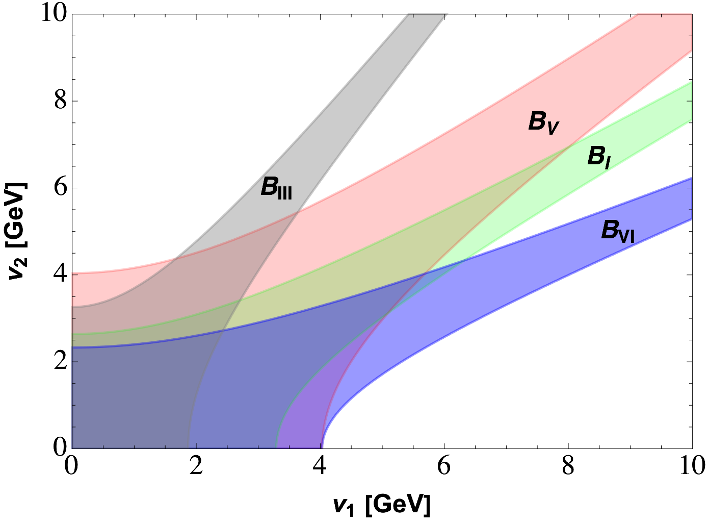
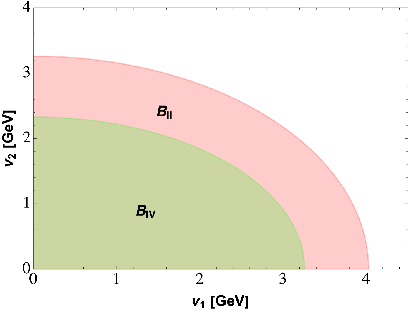
The allowed regions for each scenario are displayed in Fig. 4. As can be observed, two shapes for the allowed regions in the plane emerge. We can understand them as follows. If the condition
| (33) |
holds for both and , the allowed region is the area included in an ellipse of equation . On the other hand, if the condition of Eq. (33) holds only for or , the allowed region is the area delimited by two hyperbolae of equations . In both cases, the coefficient is a function of the parameter, the Fermi constant and the quantum numbers of the new scalar field .
| Scenario | Region | Induced VEVs | ||
| Hyperbola | 3.3 | 2.6 | ✔ | |
| Ellipse | 4.0 | 3.3 | ||
| Hyperbola | 1.9 | 3.3 | ✘ | |
| Ellipse | 3.3 | 2.3 | ✘ | |
| Hyperbola | 4.0 | 4.0 | ✔ | |
| Hyperbola | 4.0 | 2.3 |
Using this information, we can infer bounds on the VEV values.
When the allowed region is an ellipse (scenarios and ), the values of the two semi-axes correspond to the maximum values that the VEVs can assume. On the other hand, when the allowed region is the space between two hyperbolae (scenarios , , and ), the BSM VEVs can in principle also have large values if there is some partial cancellation among the contributions. However, they cannot exceed the limit imposed by the Fermi constant, namely 174 GeV. Moreover, given that the mass of the top quark is proportional to the SM Higgs VEV , by perturbativity the latter is not allowed to be too small. Thus, the new VEVs and also for the scenarios cannot exceed roughly .
Analogous to the case of class-A scenarios, we can deduce the energy scale of the new physics imposing that neutrino masses are and that the Wilson coefficients are of . Since for class-B scenarios we can have the dimension-5 operator from which , we obtain for all the scenarios, an energy scale GeV. The semi-axes of the conics which represent the allowed region for the new scalar VEVs obtained from EWPT for the class-B scenarios are listed in Table 5. Notice that in scenario the Wilson coefficients for and related to neutrino masses are not zero; given that the particle content of scenario is the same as the class-A scenarios, the new physics energy scale related to and for can be read in the discussion above. In this scenario, if all the operators are generated with Wilson coefficients, should be the largest, i.e., GeV.
3.4 Naturally-induced small VEVs
As studied above, EWPT constrain the VEVs of the new scalar multiplets to be much smaller than the Higgs doublet one. A natural way to have suppressed VEVs for the new multiplets is that they are induced by the Higgs doublet one through linear terms of the new fields in the potential. For the scenarios in which a linear term (with a trilinear dimensionful coupling) or (with a dimensionless quartic coupling) is present, a small induced VEV will be generated,
| (34) | ||||
| (35) |
where is the mass of the scalar multiplet . In Section 3.1 we have defined the conditions under which these terms exist in the potential: requires that is a triplet, while requires a quadruplet. We also showed that, regardless of the SU(2) representation, in our class-B scenarios there always exists the mixed term (see Eq. (16)). This would allow to induce a VEV for (or which will be suppressed with respect to (),
| (36) |
Summarizing, we have (see also Table 3):
- •
-
•
In the scenario, where we have two different quadruplets, there are both quartic linear terms ( and terms in Table 3 for and ) and a mixed term proportional to . Again, in this case both VEVs can be induced by the two quartic terms, see Eq. (35), and are naturally suppressed. Another possibility is to induce one of the two VEVs with the the first two terms and the second one with the mixed term. As already mentioned, it is expected that the VEV induced by the last term, Eq. (36), is subdominant.
-
•
In our and scenarios, the triplet may have a linear term proportional to in both cases, but not the quintuplet . However, a mixed term between the triplet and the quintuplet is always contained in the potential, proportional to . Thus, may be induced by the first term, Eq. (34), while by the mixed one, Eq. (36), therefore both are naturally suppressed.
-
•
When none of the scalars are in the doublet, triplet or quadruplet representations, namely for the and scenarios, we only have the mixed term with in Eq. (16). Thus, we can write a relation between the two BSM VEVs suppressing one of the two, but both of them cannot be naturally suppressed. In these scenarios, therefore, it is less natural to have small VEVs.
-
•
In scenario , where and are triplets, the scalar potential contains linear terms with two SM Higgses (with and as couplings for and ) and a mixed term with both new multiplets proportional to , see Eq. (16). In this scenario the two small VEVs can be directly induced by the SM Higgs via the first two potential terms proportional to and . Another possibility is to induce the VEV for one of the scalars via the linear term first and the second one using the mixed term. Typically, in the latter case the second VEV is smaller than the first.
We point out the presence of small induced VEVs in the last column of the Tables 4 and 5. We use the symbols ✔, and ✘ to signal that both, only one and no VEVs are induced by the linear terms in the scalar potential, respectively. In Appendix A we report for each scenario the exact expressions for neutrino masses from the small induced VEVs.
4 Phenomenology
In this section we study the phenomenological signatures associated to the different scalars present in the new operators. Given that perturbative unitarity constraints and some signals like depend on couplings of the scalar potential are mostly independent of neutrino masses and have been studied elsewhere for similar scenarios Arhrib:2011vc ; Chiang:2012qz ; Picek:2012ei ; Ghosh:2018drw , we will mainly focus on the signals of the new scalar multiplets at colliders and in EWPTs at loop level, which are directly related to neutrino masses.
4.1 Collider searches of multiply-charged scalars
The presence of multiple charged scalars belonging to different multiplets can lead to interesting phenomenological signatures at colliders. All the scenarios contain doubly-charged scalars, and except for and , all the scenarios also contain a triply-charged scalar. Furthermore, contains a quadruply-charged scalar. We are mainly interested in the phenomenology of scalars with charges 2 and above (), the decays of which can lead to multi-lepton events. Therefore, we do not consider the triplet in the analysis below. The other triplet in our scenarios, , has been widely studied in the literature in the context of Type-II seesaw (see Refs. Garayoa:2007fw ; FileviezPerez:2008jbu ; Aoki:2011pz ), and is also not discussed in the analysis below. Also, we will assume that the scalars do not mix among themselves or with any other scalars in the scenario, which is justified given that the new VEVs are much smaller than the SM Higgs one.
4.1.1 Production
The multiply-charged scalars can be pair-produced at the LHC via the Drell-Yann (DY) mechanism with an -channel exchange, whereas the associated production of the scalars involves an -channel boson exchange.555The scalars can also be photo-produced by photon fusion, e.g. via . The squared matrix element for these processes is proportional to the fourth power of the charge and thus the cross-section is enhanced for scalars with large charges. These processes can be dominant for large masses and enhance the cross section by an order of magnitude for multiply charged scalars. However, given the small parton density of photon and the large uncertainty associated with these processes, we do not consider them in the following. It can take place from a quark-antiquark initial state as
| (37) |
These cross sections depend mainly on the mass and quantum numbers of the scalars (hypercharge and isospin of the multiplet), and due to being -channel they are suppressed for heavier masses.
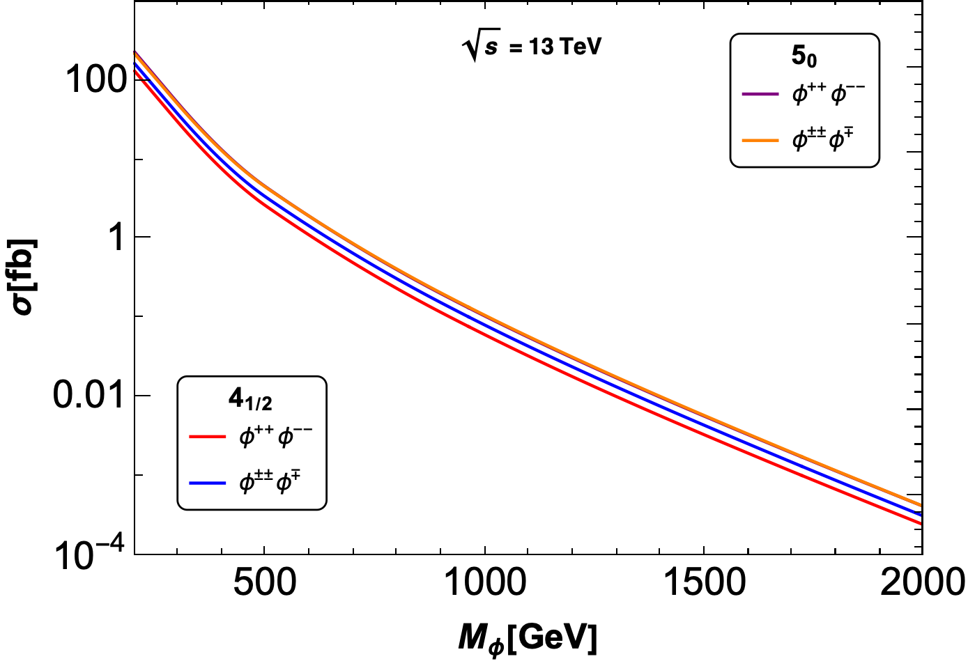
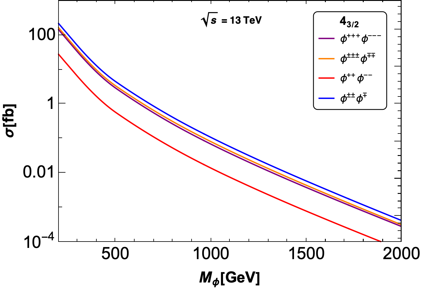
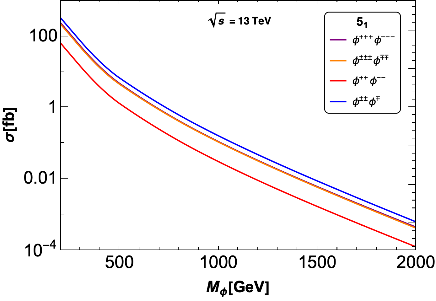
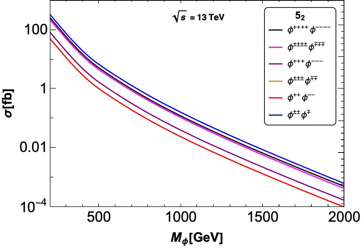
We implement the models in SARAH Staub:2013tta and numerically compute the cross-sections in MadGraph5_amC@NLO Alwall:2014hca using the NNPDF23_nlo_as_0119 PDF set Ball:2013hta . The production cross sections for the charged scalars belonging to different multiplets at the LHC (for TeV), as a function of the scalar mass, are shown in Fig. 5.
4.1.2 Decays
In this section, we discuss the decay modes of doubly, triply and quadruply-charged scalars. For scenarios belonging to class- which contain two new scalars, we take their masses to be similar so that one does not decay into the other. First, we focus solely on the decays of doubly-charged scalars, which can lead to interesting signals such as same-sign dilepton events, which are free of SM background. The effective interaction between a doubly-charged scalar () belonging to the multiplet and a pair of leptons of the same charge () can be obtained from the operator by choosing a particular contraction. This coupling can be expressed in terms of the neutrino mass matrix elements which are proportional to and would also depend on the mass ordering (normal or inverted). It can be written as
| (38) |
where is a scenario-dependent numerical factor given in Table 6 and is the VEV taken by the neutral component of the multiplet . Similarly, if the other multiplet also contains a doubly-charged component and the tensor expansion in terms of the multiplet components contains the term , we can simply make the substitution in the above formula to obtain the respective effective coupling. Note the inverse dependence on the VEV of the scalar. A large scalar VEV would highly suppress these decays, and the dominant decay channel for the doubly-charged scalars would be into a pair of bosons, which is directly proportional to the square of the VEV.
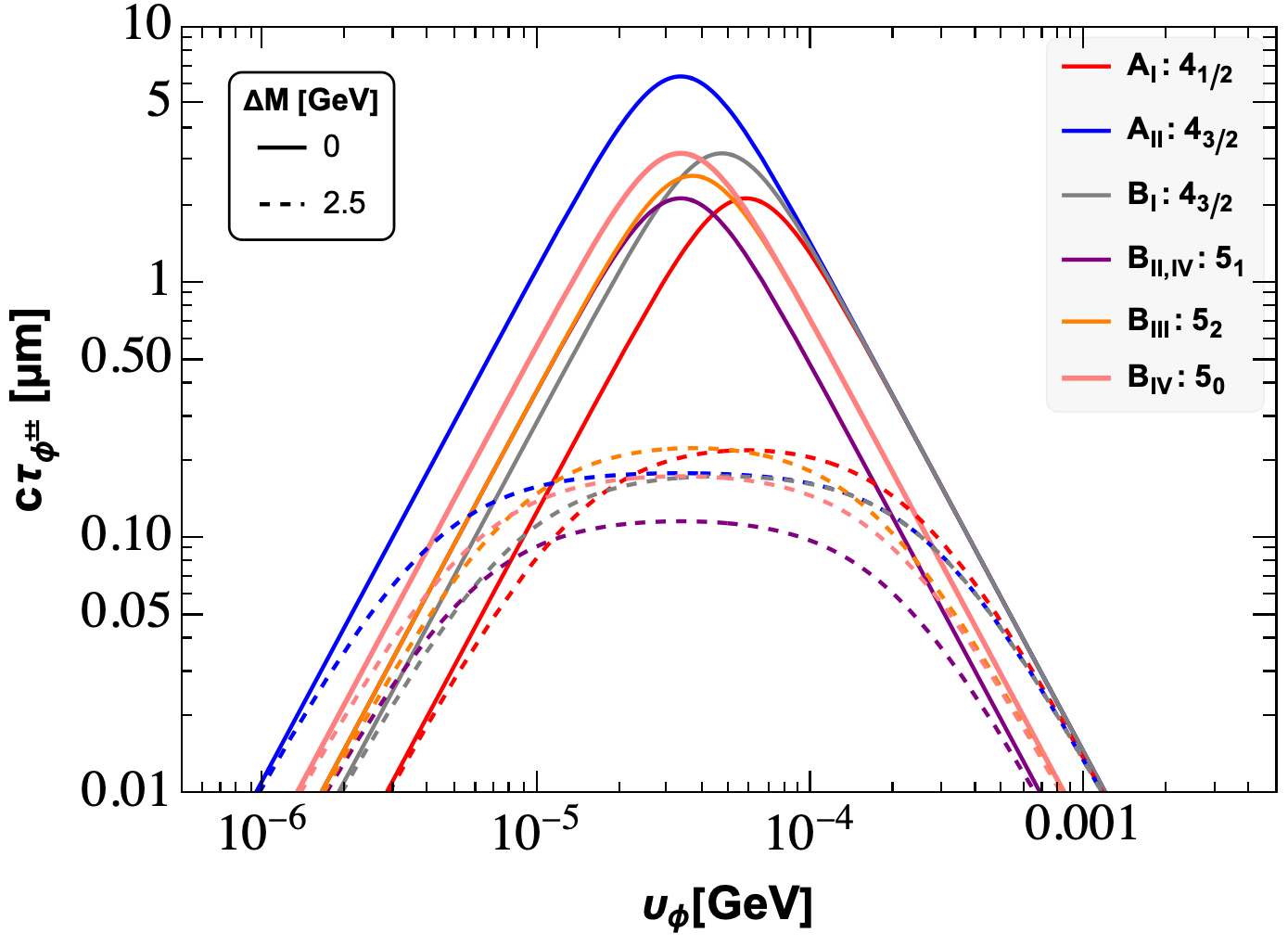
Furthermore, depending on the mass splitting between the scalar components, cascade decays () can become important, for example, decays into pions. As we show below in Section 4.2, the mass splittings between the scalars need to be small ( GeV) in order to satisfy the SM data, whereas, in the case of CDF data CDF:2022hxs , the splittings are constrained to be between GeV. Therefore, in the latter case, the cascade decays might be important for a range of VEVs. However, in both cases, we take the scalar masses to be much greater than the splittings, so the decay into solely scalar states are suppressed.
The decay rates of doubly-charged scalars belonging to quadruplet and quintuplet representations into the different channels can be scaled by comparing to the decays of a doubly-charged scalar belonging to a scalar triplet () as Ghosh:2018drw
| (39) |
where is the individual mass of active neutrinos, is the coupling, is the mass splitting among the components and is the scenario dependent factor related to the couplings and , respectively (see Table 6), MeV is the pion decay constant and . We have also dropped the index and use to denote the VEV of the scalar under consideration.
| Couplings and scale factors | ||||||
| Scenario | Scalar | |||||
| 1 | ||||||
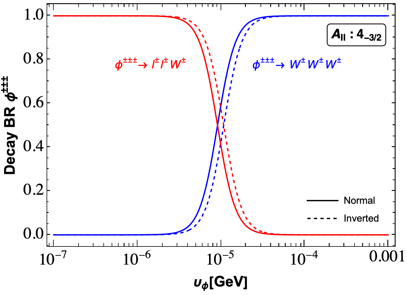
In the left (right) panel of Fig. 6 we show the branching ratio into different modes (proper decay length) of the doubly-charged scalar belonging to the multiplet of (for all scenarios) as a function of the VEV of the multiplet. We take and mass splitting GeV in the left (right) panels. The grey curves on the left panel denote the cascade decays into pions, leptons and quarks.
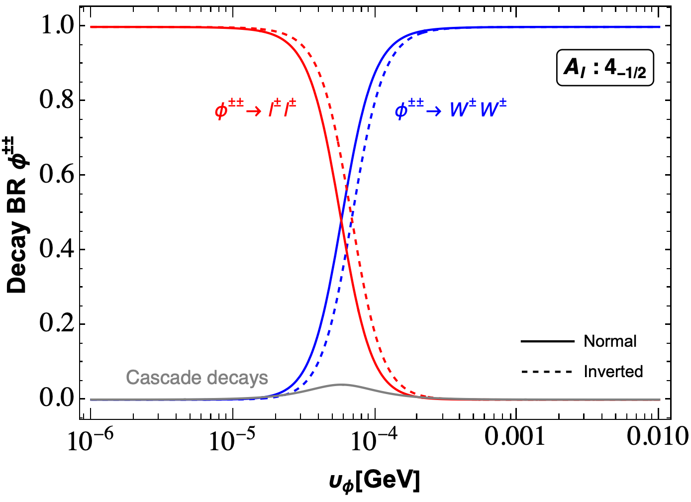
It can be seen that, for small mass splitting, the cascade decays are suppressed, and the dominant decay modes are into gauge bosons and same-sign leptons. Neglecting cascade decays, the crossover from dominant decays into leptons and into gauge bosons takes place at a value of the VEV around
| (40) |
The value of VEV at which this crossover takes place also corresponds to the point where the decay length of doubly-charged scalar is maximized. Thus, one can obtain an upper limit on the decay length of scalars. In the right panel of Fig. 6 it can be seen that the maximum proper decay length () that the doubly-charged scalars can achieve is less than for GeV, corresponding to degenerate components of the multiplet. The decay length reduces for heavier masses as well as for larger mass splittings, as the cascade decays become dominant as shown by the dashed curves. It should be noted that CMS initiates the search for displaced vertices for a proper decay length of CMS:2021tkn , and thus these scalars may not give any signals in those searches. However, prompt-lepton searches could be sensitive to them for .
Next, we focus on the decays of the triply-charged scalars. Depending on the mass splitting among the components, the dominant channels for their decays would be three-body states such as or , and two-body decays into and for , which are similar to the decays of doubly-charged scalars into (one can obtain the expressions using appropriate scaling factors). The decay widths of the triply-charged scalar present in of for are
| (41) |
The expressions for triply-charged scalars belonging to other multiplets can be obtained by rescaling the above expressions using the factors for couplings , and , see Table 6.

Similar to the case of doubly-charged scalars, the decay length is maximized at the VEV corresponding to the crossover where decays to start dominating over decays to , which is given by
| (42) |
In the left (right) panel of Fig. 7 we show the branching ratio into different modes (proper decay length) of the triply-charged scalar of scenario () as a function of the VEV of the multiplet. Being three-body decays, these decay lengths are much larger than those of doubly-charged scalars and lead to displaced vertices.
Finally, we move our attention to the quadruply-charged scalar belonging to the multiplet . The decay width of these scalars are much smaller compared to other scalars in the scenarios due to phase-space suppression. Analogous to the cases discussed above, the dominant decay modes are the four body decays to and which take place via a decay into a triply-charged scalar in association with a and the subsequent decays of the triply-charged scalar. The total decay width can be approximated by comparing to the three-body decays of triply-charged scalars as Arbelaez:2019cmj
| (43) |
where accounts for the phase-space suppression for decays to body states. Hence, the decay length of quadruply-charged scalars is roughly 60 (15) times larger than that of for masses of the order GeV, thus leading to () proper decay length. Therefore, scalars with masses can give rise to displaced vertices and can be searched for at the CMS detctor, whereas heavier quadruply-charged scalars may be looked for at prompt-lepton searches. We discuss the constraints from these searches below.
4.1.3 Signatures
The production and subsequent decays of multiply-charged scalars can lead to interesting signatures of new physics at the LHC. In Table 7, we collect the decay modes of various charged scalars and the signatures that can be obtained from pair and associated production of these scalars. As discussed above, the decay modes depend on the VEV of the corresponding scalar with leptonic decays dominating over the bosonic ones for low VEVs (see Eq. 40) and vice versa. If events like are observed at the LHC, they can confirm LNV experimentally delAguila:2013yaa .
| Decays | ||||||
| ✘ | ✘ | |||||
| ✘ | ✘ | |||||
| ✘ | ✘ | |||||
| ✘ | ✘ |
Further leptonic decays of can lead to multi-lepton events with multiple same-sign leptons in the final state, which have a very small SM background. For example, the pair and associated production of quadruply-charged scalars can lead to final states with 0-8 leptons including same-sign dileptons (), tri-lepton (SS) and tetra-lepton events (SS). Moreover, the final states from the pair production of these multi-charged scalars can all lead to lepton flavor violating 4-lepton events of the form and from the on-shell/off-shell leptonic decays of the doubly-charged scalars, corresponding to the diagonal and off-diagonal matrix elements of the light neutrino mass matrix .
The ATLAS and CMS collaborations search for doubly-charged scalars in multi-lepton finals states at TeV, corresponding to an integrated luminosity of ATLAS:2022pbd and CMS:2017pet , respectively. The ATLAS search focuses on the pair production of doubly-charged scalars and their same-sign leptonic decays with in two-, three-, four-lepton channels, considering only in the final state and assuming a 100% branching ratio to leptons, with equal branching ratio to each possible leptonic channel. In the absence of any positive signal, limits can thus be imposed on the doubly-charged scalar pair production times the branching ratio to leptons to derive a lower bound on the doubly-charged scalar mass, which in the context of left-right symmetric Type-II models comes out to 1080 GeV ATLAS:2022pbd .
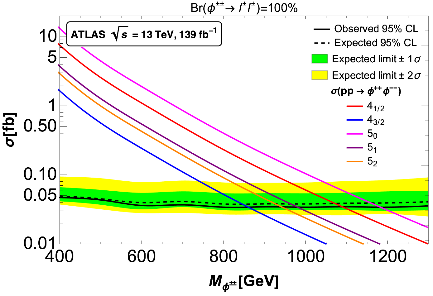
Given that the doubly-charged scalars of our scenarios exhibit similar decays, we can extend the ATLAS analysis to derive a limit on and thus on belonging to different multiplets,666Since the mass splittings among the various components of the multiplets is expected to be small from EWPTs, obtaining a bound on the doubly-charged scalar mass also gives an idea about the mass ranges of the other components of the multiplet. assuming that their induced VEV is extremely small so that . In the left plot of Fig. 8, we compare the theoretical pair production of doubly-charged scalars belonging to different multiplets (see Fig. 5) with the ATLAS results. The solid (dashed) lines represent the observed (expected) 95% CL upper limits on the pair production as a function of , and the green and yellow bands correspond to and uncertainty around the expected limit. It can be seen that GeV is excluded for the doubly-charged scalars belonging to the multiplet .
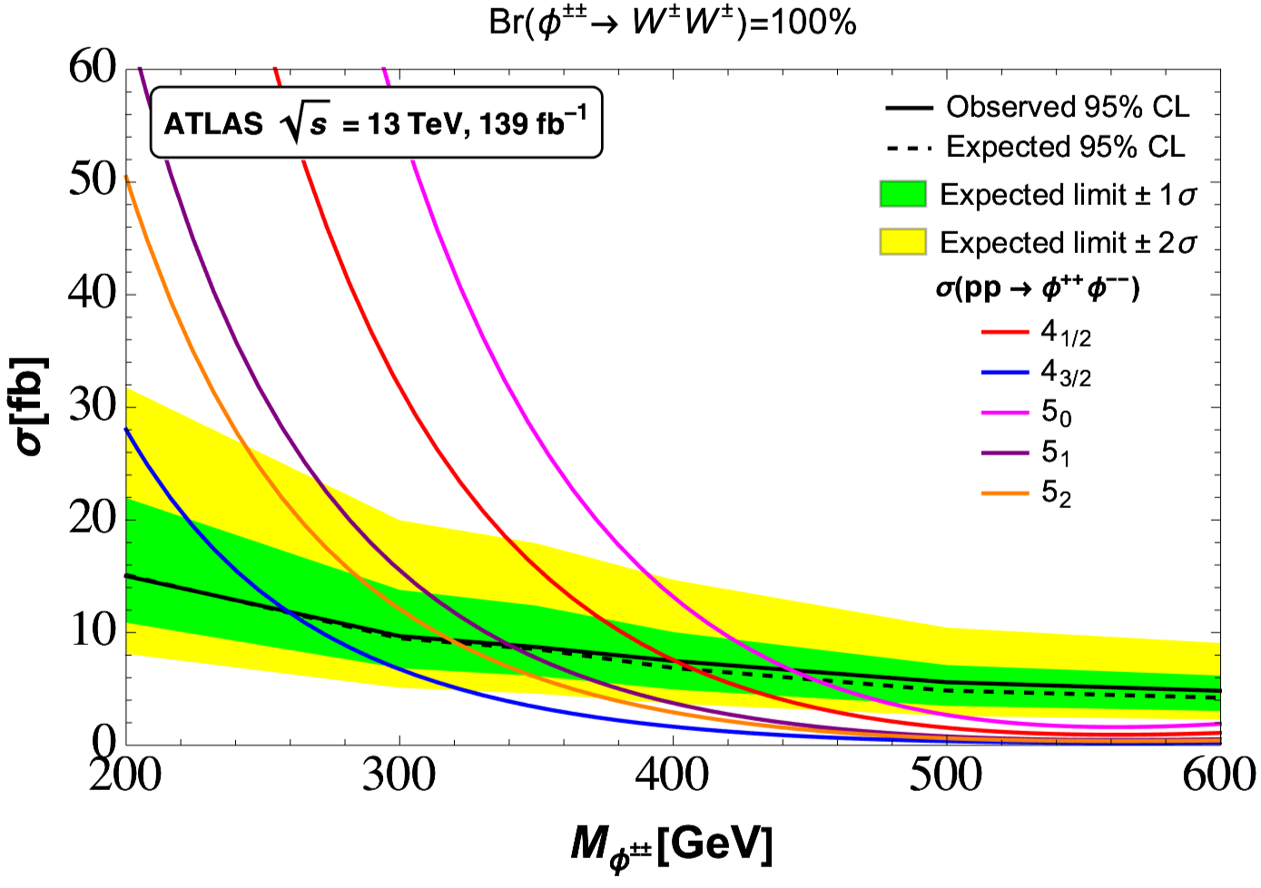
The ATLAS collaboration also searched for doubly- and singly-charged Higgs decaying into vector bosons in multi-lepton final states at TeV with an integrated luminosity of 139 , considering pair production of doubly-charged Higgs and its associated production with a singly-charged scalar in the context of the Type-II seesaw model ATLAS:2021jol . Similarly, in the absence of any deviation from SM prediction, we can extend the analysis to the doubly-charged scalars of the different multiplets to obtain naive bounds on their masses, assuming that , i.e., in the region of higher scalar VEVs. We compare the theoretical pair production cross-sections of the doubly-charged scalars with their results and show it in the right plot of Fig. 8, where the lines and bands have the same meaning as discussed above.
| Limits on | ||
| Multiplet | BR | BR |
| 1090 | 400 | |
| 860 | 260 | |
| 1180 | 440 | |
| 980 | 340 | |
| 940 | 320 | |
The lower bound on can be obtained similarly to the case above and are found to be much less stringent, for example, GeV is excluded for the doubly-charged scalars belonging to the multiplet . The exclusion limits on belonging to different multiplets from both these ATLAS searches are summarized in Table 8. These exclusion limits suffice to provide a rough estimate of the mass scales of the new scalars. These searches may help in distinguishing the doubly-charged scalars from different multiplets, since, depending on the presence of other highly-charged components in the multiplets and the mass hierarchy among them, the reconstruction of from the same-sign dilepton invariant mass may not always be possible. A study to discriminate lepton number violating scalars at the LHC, assuming that there are no excitations with was done in Ref. delAguila:2013yaa .
The search for higher-charged () scalars in the scenarios and the potential reach of the LHC in discovering them requires a more dedicated collider study in the context of a specific model and is beyond the scope of current work. We refer the reader to Refs. Bambhaniya:2013yca ; Ghosh:2018drw for the LHC phenomenology of scenario .
4.2 Electroweak Precision Tests at loop level
The addition of heavy scalar multiplets affect the oblique parameters (namely and ) that parameterize the effect of new physics on EW parameters. The new scenarios can be constrained by demanding these corrections to be small so that they do not distort the EW predictions of the SM. The oblique parameters are given by Peskin:1991sw
where is the fine structure constant, , and are the vacuum polarisation amplitudes.
The parameter, which can be written in terms of as , is equal to 1 at tree level in the SM, but can receive further corrections at the one-loop level. In our case, the leading contribution to at tree level due to addition of new scalar multiplets with isospin and hypercharge is given by Eq. (32). It can be seen that, except for scenarios containing just scalar doublets, at tree level for larger scalar multiplets obtaining VEVs, hence breaking the custodial symmetry, i.e. .
In scenarios where custodial symmetry is broken, there are complications in the calculation of oblique parameters at loop level. The parameter is divergent at one-loop level Gunion:1990dt , whereas computing and at one loop leads to either a gauge-dependent result or they become divergent as the radiative corrections that one gets in the new framework are qualitatively very different from the SM ones Jegerlehner:1991ed ; Albergaria:2021dmq . However, since we constrain the VEVs so that the parameter is close to one, we get , as discussed in Section 3.3. Therefore, the corrections to the oblique parameters can be estimated by making use of the general formulas presented in Ref. Lavoura:1993nq , where the following assumptions are made: i) the VEVs of the complex scalars are negligible, ii) the scalars do not mix with themselves or any other scalars in the theory. Both assumptions are justified for our analysis as we work in the limit , where labels the new scalar added to the SM. Further, we take as it is typically suppressed, which greatly improves the precision on and . The contribution of a scalar multiplet to the oblique parameters and is given by Lavoura:1993nq :
where is a arbitrary mass parameter used in dimensional regularization, is the hypercharge, is the weak isospin, is the third component of isospin for a multiplet with components and denotes the mass of the scalar component corresponding to it, with
| (44) |
for Mandal:2022zmy . We also discuss the implications of the addition of new scalar multiplets in alleviating the CDF anomaly related to the measurement of the boson mass777A similar study to explain the W-boson mass anomaly in terms of one loop effect of a general scalar multiplet and scalar extensions violating custodial symmetry was done in Ref. Wu:2022uwk ; Wu:2023utc ; Song:2022jns .. The correction to mass in terms of these oblique parameters (taking ) is given by Maksymyk:1993zm
| (45) |
The values of and and the correlation from the current global fit of electroweak precision data using the old (PDG 2022 ParticleDataGroup:2022pth ) and new CDF value of Lu:2022bgw are shown in Table 9.
| PDG 2022 | CDF 2022 | |
| 0.92 | 0.93 |
For the analysis below, we parameterize a scalar multiplet with components as and take the masses of the components as
| (46) |
assuming that the mass splittings among the components are equally spaced, with . In scenarios of class-, where two new scalars are involved, for the ease of analysis we take the mass of the lightest component to be the same, , and assume equal mass gaps for both multiplets, . Thus, using Eqs. (4.2) and (45), and the values given in Table 9, we can constrain the mass of the lightest component and the mass splitting by means of a two-parameter analysis. In Fig. 9 we show the EWPT bounds (at 95% C.L.) in the plane along with the bounds to reproduce the previous and the new measurement of the boson mass. The light blue (light red) region indicates the parameter space allowed by EWPT from the PDG (CDF measurement), whereas the dark blue (dark red) shows the parameter space allowed by the old (new) measurement of .
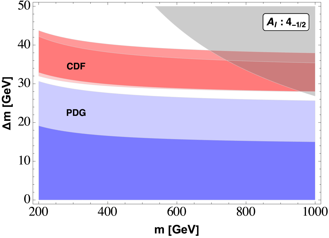
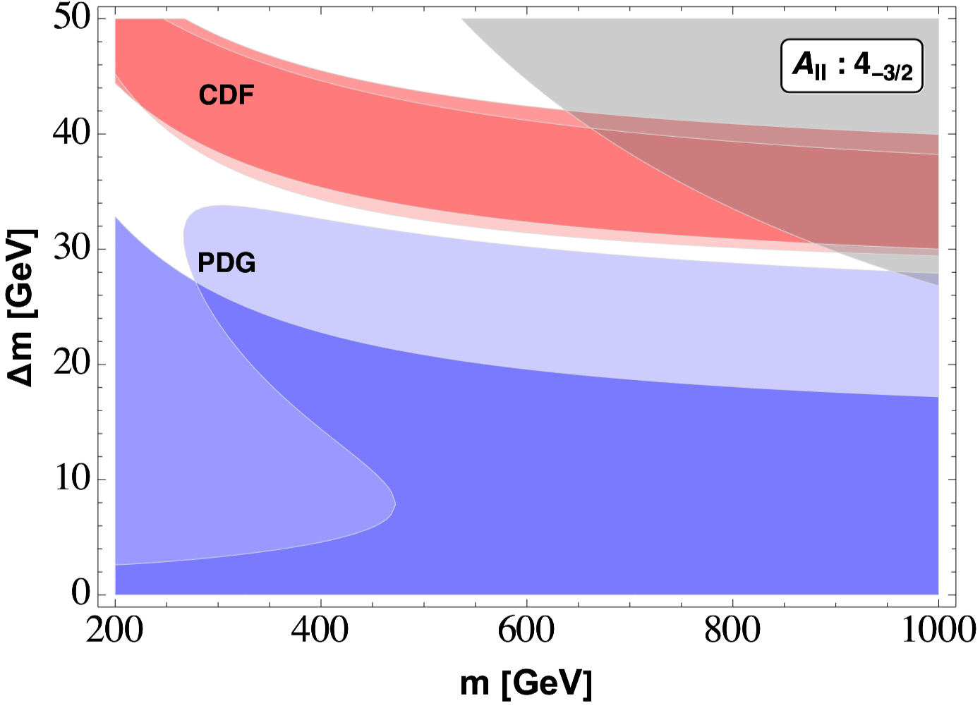

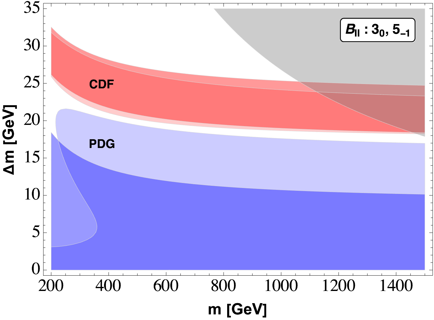
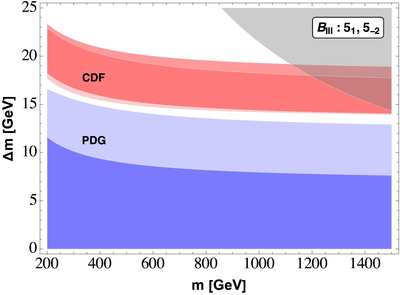
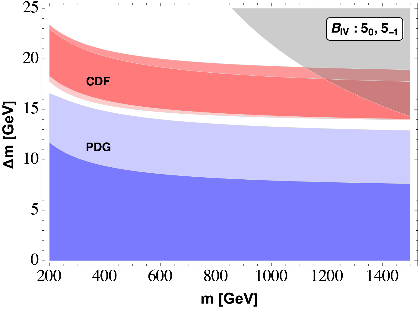
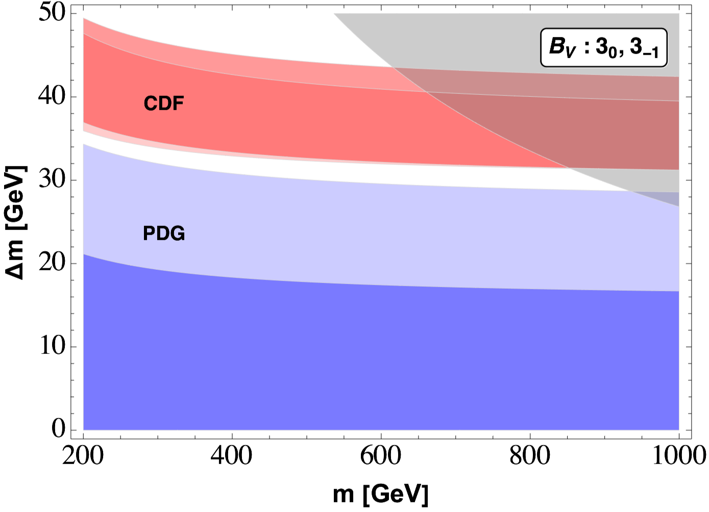
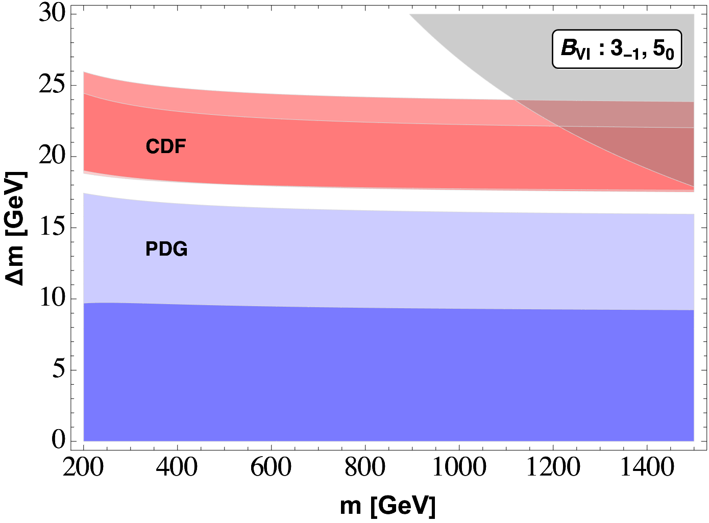
Note that the mass splitting among the components is proportional to the Higgs VEV and the quartic coupling . The mass gaps can then be parameterized as
| (47) |
where is bounded by perturbativity. We show this bound in the top right gray region in Fig. 9.
From the above estimates, it can be seen that multiplets belonging to higher representation require smaller mass splittings in order to be consistent with electroweak fits (EWPT and ). The allowed splittings are larger for the new CDF fit, as expected, since the new measurement indicates a larger value of and which is strongly disfavored by SM and is in tension with the PDG data. In class- scenarios, the CDF data points to a mass splitting of around 40 - 50 GeV for , 20 - 30 GeV for and 15 - 25 GeV for . Further, if the CDF data turns out to be correct, perturbativity excludes the new scalar masses to be larger than .
5 Conclusions
The origin of neutrino masses remains an open question. In the SM, with just the Higgs doublet, the Weinberg operator seems a very plausible indication for the Majorana nature of neutrinos. However, if this is the mechanism by which neutrinos acquire their tiny masses, it will be very difficult to test it. On the other hand, new scalar multiplets may be present at energies not far from the EW scale, and they give rise to new Weinberg-like operators. If these new scalars take VEVs, necessarily suppressed ( GeV) due to constraints from EWPTs, neutrino masses may be generated for smaller LNV scales.
In this work we study the possible Weinberg-like operators with new electroweak scalars. We consider scenarios where neutrino masses induced by the SM Weinberg operator are suppressed. These requirements leave us with possibilities with new scalar multiplets up to quintuplet SU(2) representations. We have found that, in some cases, naturally small induced VEVs are generated. Their UV completions lead to new seesaw scenarios, which are studied in a companion paper us:2023two , where we also study the one-loop contributions to neutrino masses and the phenomenology induced by the heavy fermions.
By construction, the new scalars are expected to lie not far from the EW scale, i.e., at TeV energies. Therefore, they may be produced at colliders. If the new VEVs are small enough ( keV), the neutrino mass matrix may be reconstructed from doubly-charged decays. Let us also mention that in these scenarios the electroweak phase transition may be first order, which in turn could explain the baryon asymmetry of the universe via electroweak baryogenesis. Gravitational waves may provide a way to probe this scenario. A detailed study of this possibility would be interesting to pursue.
We conclude that, if a positive signal is observed at colliders and/or a deviation is measured in EWPTs, this may point to new scalars at the TeV scale, which may well be related to the origin of neutrino masses as analysed in this work.
Acknowledgements.
We are grateful to Andrea Di Iura and Claudia Hagedorn for their participation in the early stages of this project. We also thank Anirban Karan, Emanuela Musumeci, Arcadi Santamaria and Avelino Vicente and for useful discussions. All Feynman diagrams were generated using the TikZ-Feynman package for LaTeX Ellis:2016jkw . JHG and DV are partially supported by the “Generalitat Valenciana” through the GenT Excellence Program (CIDEGENT/2020/020) and by the Spanish “Agencia Estatal de Investigación”, MICINN/AEI (10.13039/501100011033) grants PID2020-113334GB-I00 and PID2020-113644GB-I00. JHG is also supported by the “Consolidación Investigadora” Grant CNS2022-135592 funded by the Spanish “Agencia Estatal de Investigación”, MICINN/AEI (10.13039/501100011033) and by “European Union NextGenerationEU/PRTR”.Appendix A Weinberg-like operators with SM Higgs doublets
As long as , one can integrate-out the new multiplets and at low energies Weinberg-like operators with just Higgs doublets at dimension are generated Anamiati:2018cuq , of the form
| (48) |
We see that the case corresponds to the dimension- Weinberg operator. After EWSB, these Weinberg-like operators generate neutrino masses at tree level. This can also be understood from the fact that new scalars acquire an induced VEV, as discussed in Section 3.4.
Let us first consider the class-A scenarios. The effective neutrino mass for reads
| (49) |
where is the numerical factor associated with the contraction of the fields (which we report in Table 10) in the potential term linear in and is the symmetric part of the Wilson coefficients matrix associated to , as mentioned below Eq. 8. The mass dimensions of the two effective operators entering the neutrino masses in this case are and , respectively.
For the scenario, on the other hand, the neutrino mass matrix reads
| (50) |
that corresponds to operator.
| n | ||||
| ✘ | ✘ | 7, 9 | ||
| ✘ | ✘ | 7 | ||
| 7, 9, 11, 13 | ||||
| ✘ | 9 | |||
| ✘ | ✘ | 7 | ||
| ✘ | ✘ | 7 | ||
| 9, 11 | ||||
| ✘ | 9 |
Let us now move to the scenarios. The scenario is the most complicated one, since with two quadruplets we can have three types of BSM Weinberg-like operators, namely , and . Moreover, just like the previous case, we can induce both VEVs using the SM Higgs via quartic terms, or we can induce one of the two with the mixed term. If both new VEVs are induced by the Higgs, then neutrino masses read
| (51) | |||||
where it is clear that the Weinberg operator does not exist due to the -3/2 hypercharge of the second quadruplet. The effective dimension of the four operators are for the first two operators, and for the third and fourth one. If only is induced by the SM Higgs VEV while is induced via the mixing, neutrino masses read
| (52) | |||||
where the effective dimension is for the first operator, for the second and third operators and for the last one. On the other hand, if only is induced by the Higgs VEV we have a more suppressed contribution from the third term and neutrino masses are
Here the neutrino masses are obtained, in order, from , , and effective operators. Depending on the value of the Wilson coefficients , the dominant contribution can come from different terms. As an example, we show the Feynman diagram related to (left) and (right) operators in in Fig. 10.
Let us now consider the and scenarios. In this case we have only one possibility, namely that is induced by the SM Higgs while , coming from a quintuplet, can only be induced by the mixed term. We have operator from which neutrino masses can be written as
| (54) |
For the scenarios, and , as discussed in the previous section, there does not exist a mechanism which ensures that both the VEVs are naturally small. However, neutrino masses may still arise from operator, for instance, induced by (i.e., ),
| (55) |
In the opposite case the neutrino mass matrix can be obtained with the substitutions and .
Finally, for the , neutrino masses could arise from a or operator, depending on how the new multiplets VEVs are induced. If both of the VEVs are induced from SM Higgs one, we obtain a dimension- operator, which gives the following neutrino mass
| (56) |
where is the symmetric part of the Wilson coefficients matrix associated to , and are the numerical factors (see Table 10) related to the contractions of the and terms, respectively. On the other hand, if one of the two VEV is induced by the SM Higgs while the second one is induced by the mixed term , neutrino masses arise from a dimension- operator and they read
| (57) |
where now is the numerical factor related to the contraction of the mixed potential term. In this case we expect . If the second scalar multiplet VEV is the one induced directly by the Higgs, neutrino masses are obtained from Eq. (57) with the substitutions , and .
All the numerical coefficients arising from the contraction of the potential terms that induce the small VEVs are reported, as already mentioned, in Table 10 along with the mass dimension at which the neutrino masses are generated.
Appendix B Tensor contractions
We define here in tensor notation the lepton number violating potential terms in scenario (see Table 3), calling for simplicity and
| (58) | ||||
References
- (1) S. Weinberg, Baryon and Lepton Nonconserving Processes, Phys.Rev.Lett. 43 (1979) 1566.
- (2) P. Minkowski, at a Rate of One Out of Muon Decays?, Phys. Lett. B 67 (1977) 421.
- (3) T. Yanagida, Horizontal Symmetry and Masses of Neutrinos, Prog. Theor. Phys. 64 (1980) 1103.
- (4) M. Gell-Mann, P. Ramond and R. Slansky, Complex Spinors and Unified Theories, Conf. Proc. C 790927 (1979) 315 [1306.4669].
- (5) R.N. Mohapatra and G. Senjanovic, Neutrino Mass and Spontaneous Parity Nonconservation, Phys. Rev. Lett. 44 (1980) 912.
- (6) J. Schechter and J.W.F. Valle, Neutrino Masses in SU(2) x U(1) Theories, Phys. Rev. D 22 (1980) 2227.
- (7) J. Schechter and J.W.F. Valle, Neutrino Decay and Spontaneous Violation of Lepton Number, Phys. Rev. D 25 (1982) 774.
- (8) G. Lazarides, Q. Shafi and C. Wetterich, Proton Lifetime and Fermion Masses in an SO(10) Model, Nucl. Phys. B 181 (1981) 287.
- (9) R.N. Mohapatra and G. Senjanovic, Neutrino Masses and Mixings in Gauge Models with Spontaneous Parity Violation, Phys. Rev. D 23 (1981) 165.
- (10) R. Foot, H. Lew, X.G. He and G.C. Joshi, Seesaw Neutrino Masses Induced by a Triplet of Leptons, Z. Phys. C 44 (1989) 441.
- (11) K.S. Babu and C.N. Leung, Classification of effective neutrino mass operators, Nucl. Phys. B 619 (2001) 667 [hep-ph/0106054].
- (12) A. de Gouvea and J. Jenkins, A Survey of Lepton Number Violation Via Effective Operators, Phys. Rev. D77 (2008) 013008 [0708.1344].
- (13) A. de Gouvea, J. Herrero-Garcia and A. Kobach, Neutrino Masses, Grand Unification, and Baryon Number Violation, Phys.Rev. D90 (2014) 016011 [1404.4057].
- (14) P.W. Angel, N.L. Rodd and R.R. Volkas, Origin of neutrino masses at the LHC: effective operators and their ultraviolet completions, Phys. Rev. D 87 (2013) 073007 [1212.6111].
- (15) F. del Aguila, A. Aparici, S. Bhattacharya, A. Santamaria and J. Wudka, Effective Lagrangian approach to neutrinoless double beta decay and neutrino masses, JHEP 06 (2012) 146 [1204.5986].
- (16) J. Gargalionis and R.R. Volkas, Exploding operators for Majorana neutrino masses and beyond, JHEP 01 (2021) 074 [2009.13537].
- (17) J. Herrero-García and M.A. Schmidt, Neutrino mass models: New classification and model-independent upper limits on their scale, Eur. Phys. J. C 79 (2019) 938 [1903.10552].
- (18) A. Giarnetti, J. Herrero-Garcia, S. Marciano, D. Meloni and D. Vatsyayan, Neutrino masses from new Weinberg-like operators: Phenomenology of the seesaw completions, In preparation .
- (19) F. Bonnet, D. Hernandez, T. Ota and W. Winter, Neutrino masses from higher than d=5 effective operators, JHEP 10 (2009) 076 [0907.3143].
- (20) R. Cepedello, M. Hirsch and J.C. Helo, Lepton number violating phenomenology of d = 7 neutrino mass models, JHEP 01 (2018) 009 [1709.03397].
- (21) G. Anamiati, O. Castillo-Felisola, R.M. Fonseca, J.C. Helo and M. Hirsch, High-dimensional neutrino masses, JHEP 12 (2018) 066 [1806.07264].
- (22) K.L. McDonald, Minimal Tree-Level Seesaws with a Heavy Intermediate Fermion, JHEP 07 (2013) 020 [1303.4573].
- (23) S.S.C. Law and K.L. McDonald, A Class of Inert N-tuplet Models with Radiative Neutrino Mass and Dark Matter, JHEP 09 (2013) 092 [1305.6467].
- (24) W. Wang and Z.-L. Han, Naturally Small Dirac Neutrino Mass with Intermediate Multiplet Fields, JHEP 04 (2017) 166 [1611.03240].
- (25) K. Hally, H.E. Logan and T. Pilkington, Constraints on large scalar multiplets from perturbative unitarity, Phys. Rev. D 85 (2012) 095017 [1202.5073].
- (26) S. Dawson and C.W. Murphy, Standard Model EFT and Extended Scalar Sectors, Phys. Rev. D 96 (2017) 015041 [1704.07851].
- (27) H.E. Logan and M.-A. Roy, Higgs couplings in a model with triplets, Phys. Rev. D 82 (2010) 115011 [1008.4869].
- (28) G. Durieux, G. Durieux, M. McCullough, M. McCullough, E. Salvioni and E. Salvioni, Charting the Higgs self-coupling boundaries, JHEP 12 (2022) 148 [2209.00666].
- (29) K. Kannike, Constraining the Higgs Trilinear Coupling from an Quadruplet with Bounded-from-Below Conditions, 2311.17995.
- (30) E. Ma, Verifiable radiative seesaw mechanism of neutrino mass and dark matter, Phys. Rev. D 73 (2006) 077301 [hep-ph/0601225].
- (31) Y. Cai, J. Herrero-García, M.A. Schmidt, A. Vicente and R.R. Volkas, From the trees to the forest: a review of radiative neutrino mass models, Front.in Phys. 5 (2017) 63 [1706.08524].
- (32) M. Fierz, Zur Fermischen Theorie des -Zerfalls, Z. Phys. 104 (1937) 553.
- (33) T.D. Lee, A Theory of Spontaneous T Violation, Phys. Rev. D 8 (1973) 1226.
- (34) G.C. Branco, P.M. Ferreira, L. Lavoura, M.N. Rebelo, M. Sher and J.P. Silva, Theory and phenomenology of two-Higgs-doublet models, Phys. Rept. 516 (2012) 1 [1106.0034].
- (35) J.F. Oliver and A. Santamaria, Neutrino masses from operator mixing, Phys. Rev. D 65 (2002) 033003 [hep-ph/0108020].
- (36) J. Hernandez-Garcia and S.F. King, New Weinberg operator for neutrino mass and its seesaw origin, JHEP 05 (2019) 169 [1903.01474].
- (37) K. Earl, K. Hartling, H.E. Logan and T. Pilkington, Constraining models with a large scalar multiplet, Phys. Rev. D 88 (2013) 015002 [1303.1244].
- (38) Y. Chikashige, R.N. Mohapatra and R.D. Peccei, Are There Real Goldstone Bosons Associated with Broken Lepton Number?, Phys. Lett. B 98 (1981) 265.
- (39) G.B. Gelmini and M. Roncadelli, Left-Handed Neutrino Mass Scale and Spontaneously Broken Lepton Number, Phys. Lett. B 99 (1981) 411.
- (40) M.A. Diaz, M.A. Garcia-Jareno, D.A. Restrepo and J.W.F. Valle, Seesaw Majoron model of neutrino mass and novel signals in Higgs boson production at LEP, Nucl. Phys. B 527 (1998) 44 [hep-ph/9803362].
- (41) P. Escribano, M. Hirsch, J. Nava and A. Vicente, Observable flavor violation from spontaneous lepton number breaking, JHEP 01 (2022) 098 [2108.01101].
- (42) CMS collaboration, Precision measurement of the Z boson invisible width in pp collisions at s=13 TeV, Phys. Lett. B 842 (2023) 137563 [2206.07110].
- (43) M.J.G. Veltman, Limit on Mass Differences in the Weinberg Model, Nucl. Phys. B 123 (1977) 89.
- (44) P. Sikivie, L. Susskind, M.B. Voloshin and V.I. Zakharov, Isospin Breaking in Technicolor Models, Nucl. Phys. B 173 (1980) 189.
- (45) Particle Data Group collaboration, Review of Particle Physics, PTEP 2022 (2022) 083C01.
- (46) CDF collaboration, High-precision measurement of the boson mass with the CDF II detector, Science 376 (2022) 170.
- (47) P. Langacker, Grand Unified Theories and Proton Decay, Phys. Rept. 72 (1981) 185.
- (48) A. Arhrib, R. Benbrik, M. Chabab, G. Moultaka and L. Rahili, Higgs boson decay into 2 photons in the type~II Seesaw Model, JHEP 04 (2012) 136 [1112.5453].
- (49) C.-W. Chiang and K. Yagyu, Higgs boson decays to and Z in models with Higgs extensions, Phys. Rev. D 87 (2013) 033003 [1207.1065].
- (50) I. Picek and B. Radovcic, Enhancement of by seesaw-motivated exotic scalars, Phys. Lett. B 719 (2013) 404 [1210.6449].
- (51) T. Ghosh, S. Jana and S. Nandi, Neutrino mass from Higgs quadruplet and multicharged Higgs searches at the LHC, Phys. Rev. D 97 (2018) 115037 [1802.09251].
- (52) J. Garayoa and T. Schwetz, Neutrino mass hierarchy and Majorana CP phases within the Higgs triplet model at the LHC, JHEP 03 (2008) 009 [0712.1453].
- (53) P. Fileviez Perez, T. Han, G.-y. Huang, T. Li and K. Wang, Neutrino Masses and the CERN LHC: Testing Type II Seesaw, Phys. Rev. D 78 (2008) 015018 [0805.3536].
- (54) M. Aoki, S. Kanemura and K. Yagyu, Testing the Higgs triplet model with the mass difference at the LHC, Phys. Rev. D 85 (2012) 055007 [1110.4625].
- (55) F. Staub, SARAH 4 : A tool for (not only SUSY) model builders, Comput. Phys. Commun. 185 (2014) 1773 [1309.7223].
- (56) J. Alwall, R. Frederix, S. Frixione, V. Hirschi, F. Maltoni, O. Mattelaer et al., The automated computation of tree-level and next-to-leading order differential cross sections, and their matching to parton shower simulations, JHEP 07 (2014) 079 [1405.0301].
- (57) NNPDF collaboration, Parton distributions with QED corrections, Nucl. Phys. B 877 (2013) 290 [1308.0598].
- (58) CMS collaboration, Search for long-lived particles decaying to jets with displaced vertices in proton-proton collisions at 13 TeV, Phys. Rev. D 104 (2021) 052011 [2104.13474].
- (59) C. Arbeláez, J.C. Helo and M. Hirsch, Long-lived heavy particles in neutrino mass models, Phys. Rev. D 100 (2019) 055001 [1906.03030].
- (60) F. del Aguila, M. Chala, A. Santamaria and J. Wudka, Discriminating between lepton number violating scalars using events with four and three charged leptons at the LHC, Phys. Lett. B 725 (2013) 310 [1305.3904].
- (61) ATLAS collaboration, Search for doubly charged Higgs boson production in multi-lepton final states using 139 fb-1 of proton-proton collisions at = 13 TeV with the ATLAS detector, 2211.07505.
- (62) CMS collaboration, A search for doubly-charged Higgs boson production in three and four lepton final states at , .
- (63) ATLAS collaboration, Search for doubly and singly charged Higgs bosons decaying into vector bosons in multi-lepton final states with the ATLAS detector using proton-proton collisions at = 13 TeV, JHEP 06 (2021) 146 [2101.11961].
- (64) G. Bambhaniya, J. Chakrabortty, S. Goswami and P. Konar, Generation of neutrino mass from new physics at TeV scale and multilepton signatures at the LHC, Phys. Rev. D 88 (2013) 075006 [1305.2795].
- (65) M.E. Peskin and T. Takeuchi, Estimation of oblique electroweak corrections, Phys. Rev. D 46 (1992) 381.
- (66) J.F. Gunion, R. Vega and J. Wudka, Naturalness problems for rho = 1 and other large one loop effects for a standard model Higgs sector containing triplet fields, Phys. Rev. D 43 (1991) 2322.
- (67) F. Jegerlehner, Physics of precision experiments with Zs, Prog. Part. Nucl. Phys. 27 (1991) 1.
- (68) F. Albergaria and L. Lavoura, Prescription for finite oblique parameters S and U in extensions of the SM with m W m Z cos W, J. Phys. G 49 (2022) 085005 [2111.02339].
- (69) L. Lavoura and L.-F. Li, Making the small oblique parameters large, Phys. Rev. D 49 (1994) 1409 [hep-ph/9309262].
- (70) S. Mandal, O.G. Miranda, G. Sanchez Garcia, J.W.F. Valle and X.-J. Xu, Toward deconstructing the simplest seesaw mechanism, Phys. Rev. D 105 (2022) 095020 [2203.06362].
- (71) J. Wu, D. Huang and C.-Q. Geng, W-boson mass anomaly from a general SU(2)L scalar multiplet*, Chin. Phys. C 47 (2023) 063103 [2212.14553].
- (72) J. Wu, C.-Q. Geng and D. Huang, -boson Mass Anomaly from High-Dimensional Scalar Multiplets, 2307.12105.
- (73) H. Song, X. Wan and J.-H. Yu, Custodial symmetry violation in scalar extensions of the standard model*, Chin. Phys. C 47 (2023) 103103 [2211.01543].
- (74) I. Maksymyk, C.P. Burgess and D. London, Beyond S, T and U, Phys. Rev. D 50 (1994) 529 [hep-ph/9306267].
- (75) C.-T. Lu, L. Wu, Y. Wu and B. Zhu, Electroweak precision fit and new physics in light of the W boson mass, Phys. Rev. D 106 (2022) 035034 [2204.03796].
- (76) J. Ellis, TikZ-Feynman: Feynman diagrams with TikZ, Comput. Phys. Commun. 210 (2017) 103 [1601.05437].