Improving fidelity of multi-qubit gates using hardware-level pulse parallelization

Abstract

Quantum computation holds the promise of solving computational problems which are believed to be classically intractable. However, in practice, quantum devices are still limited by their relatively short coherence times and imperfect circuit-hardware mapping. In this work, we present the parallelization of pre-calibrated pulses at the hardware level as an easy-to-implement strategy to optimize quantum gates. Focusing on $R_{ZX}^{\mathrm{\,}}$ gates, we demonstrate that such parallelization leads to improved fidelity and gate time reduction, when compared to serial concatenation. As measured by Cycle Benchmarking, our most modest fidelity gain was from 98.16(7)% to 99.15(3)% for the application of two $R_{ZX}^{\mathrm{\,}}(\pi/2)$ gates with one shared qubit. We show that this strategy can be applied to other gates like the CNOT and CZ, and it may benefit tasks such as Hamiltonian simulation problems, amplitude amplification, and error-correction codes.

I Introduction

The field of quantum computing has seen an explosion of interest in the recent decades [nature2022editorial, Bravyi2022, nielsenQuantumComputationQuantum2012]. Seminal results such as Shor’s algorithm [shor_discrete_log, shor_factoring, nielsenQuantumComputationQuantum2012] and the threshold theorem for Quantum Error Correction [Devitt_2013, gottesman1997stabilizer, Ali07, aharonov1997fault] have provided the hope that quantum computers may one day solve problems that are currently intractable [nielsenQuantumComputationQuantum2012].

One major limitation to the field of quantum computation is that the quantum circuit abstraction breaks down when one uses real quantum devices. Physically, unitaries are only implemented approximately, using classical fields, and the resulting operation will not match the expected one with perfect fidelity [glaserTrainingSchrodingerCat2015, kochChargeinsensitiveQubitDesign2007a]. Furthermore, when designing quantum circuits, the circuit implementation is not tailored to some specific hardware. The circuit gates may be mapped sub-optimally to the pulse-level instruction schedule, thereby leading to longer pulse instructions and higher decoherence [sundaresanReducingUnitarySpectator2020, kimHighfidelityThreequbitIToffoli2022, alexanderQiskitPulseProgramming2020, nguyenBlueprintHighPerformanceFluxonium2022, ibrahimEvaluationParameterizedQuantum2022].

In fact, another main limitation of noisy intermediate-scale quantum (NISQ) devices is their relatively short coherence times [Preskill2018quantumcomputingin]. As the physical apparatus encoding the quantum state quickly interacts with the environment and suffers decoherence, there is a limited window where quantum operations can be performed on the quantum state, while still retaining acceptable fidelity. The rapid decoherence imposes limits on the circuit depths that are practically viable, and the number of gates applied, which limits the complexity of the quantum circuits that can be implemented in practice. This constraint ultimately limits the practical usefulness of quantum computing to solve problems where there is an expected theoretical quantum advantage. Consequently, in order to make the most use of current NISQ devices, we are compelled to shorten circuit times whenever possible, thereby enabling us to implement more complex circuits in the same time window.

Various approaches have been proposed to map abstract quantum circuits to efficient and fast pulse-level instructions. Transpilation, for instance, relies on gate cancellation and simplification, using optimization techniques [namAutomatedOptimizationLarge2018], and takes into account known connectivity constraints in the quantum device of interest, leading to a mapping that requires fewer intermediate gates to provide the desired connectivity, such as SWAP gates. At a lower level, circuit compilation [earnestPulseefficientCircuitTranspilation2021, stengerSimulatingDynamicsBraiding2021] tries to decompose the original quantum circuit in terms of quantum gates that are less common but more representative of the underlying physical system. Finally, at the lowest level, we may use quantum control [dalessandroIntroductionQuantumControl2021] and work with the pulse-level implementation directly, which might be the optimal policy to ensure high fidelities. However, this comes with significant trade-offs. The pulses that can be directly implemented in the superconducting qubits, for instance, do not map to commonly used quantum gates [kochChargeinsensitiveQubitDesign2007a]. As a result, building large quantum circuits by using these pulse gates directly would be unintuitive and impractical.

In this work, we present an optimization strategy that lies between compilation and quantum control and that is readily available in contemporary devices—parallelization of pre-calibrated pulses. Following this procedure, we are able to map unitaries to native instructions, reduce gate times and increase fidelity, all with minimal effort. We show in section II that many Hamiltonian simulation problems can benefit from such a parallelization. One particular realization of this strategy relies on parallelizing $R_{ZX}^{\mathrm{\,}}(\theta)$ gates with a shared qubit. In section III we present the parallelization strategy and demonstrate that the Parallel $R_{ZX}^{\mathrm{\,}}$ gate, $P_{abc}^{\mathrm{\,}}(\theta)$, is natively available in real devices and that it outperforms its serial counterpart. In fact, as measured by Cycle Benchmarking, by parallelizing two $R_{ZX}^{\mathrm{\,}}(\pi/2)$ gates the fidelity goes from $98.16(7)\%$ to $99.15(3)\%$. We emphasize that the $P_{abc}^{\mathrm{\,}}(\theta)$ gates constitute a family of native high-fidelity three-qubit gates. Finally, in LABEL:sec:applications, we discuss how the parallelization strategy can be further generalized and applied to other problems.

II Pulse parallelization in NISQ Devices

Current quantum devices already heavily rely on parallelization of single qubit gates in order to achieve short circuit depths and durations (see fig. 1). In this case, the pulse-level parallelization is straightforward, as there is no pulse overlap between qubits. Similarly, multi-qubit gates can be parallelized at the pulse level if no qubits are shared among them. However, in order to harness the full advantage of quantum devices, highly entangled quantum states are required, and to create these it is necessary to apply multi-qubit gates to shared qubits, for which parallelization at the pulse level is no longer straightforward.

Fortunately, while multi-qubit gates applied to overlapping qubits cannot be parallelized at the abstract circuit layer, we show that it is possible to parallelize them at the pulse layer, and that this parallelization is straightforward to implement once recognized.

Two gates $U_{1},U_{2}$ may be parallelizable, for instance, if they are generated by two commuting time-independent Hamiltonians $H_{1}$ and $H_{2}$,

$$U_{1}U_{2}=e^{-iH_{1}t_{1}}e^{-iH_{2}t_{2}}=e^{-it(H_{1}^{\prime}+H_{2}^{\prime})}.$$ (1)

Here, $H_{i}^{\prime}=H_{i}t_{i}/t$ are re-scaled versions of the Hamiltonians. The evolution on the right-hand side happens in time $t$, which may be chosen to be less than $t_{1}+t_{2},$ as illustrated in fig. 1.

In actual quantum machines—using superconducting transmon qubits, trapped ions, or others—Hamiltonians are implemented via an external driving signal, like an electrical current or a laser [kochChargeinsensitiveQubitDesign2007a]. Therefore, if two gates commute, it is possible that their underlying pulse signals can be superposed in order to approximate the evolution in eq. 1. Of course, it is important to emphasize that in real devices we can only approximate some desired Hamiltonian, as there are usually extra interactions that break commutativity [sundaresanReducingUnitarySpectator2020, kimHighfidelityThreequbitIToffoli2022, alexanderQiskitPulseProgramming2020, nguyenBlueprintHighPerformanceFluxonium2022, ibrahimEvaluationParameterizedQuantum2022]. Additionally, implementing $H_{1}^{\prime}+H_{2}^{\prime}$ may consume more resources than $H_{1}$ and $H_{2}$ individually, and there will be practical limitations to its implementation, like voltage saturation or non-linear effects. Nevertheless, if $t$ is less than $t_{1}+t_{2}$, parallelization may help achieve a computation in a shorter time interval, relative to the system’s decoherence time, resulting in a net fidelity gain.

For this reason, it is interesting to ask whether pulse superposition can be used for gate parallelization in practice. We show that, in contemporary commercially-available quantum devices, the answer is positive.

$$\Qcircuit@C=0.8em@R=0.6em{\ar@{.}[]+<0.5em,1em>;[d]+<0.5em,-2.5em>&\gate{X}\ar@{.}[]+<1em,1em>;[d]+<1em,-2.5em>\qw\ar@{.}[]+<1em,1em>;[d]+<1em,-2.5em>\gate{X}\ar@{.}[]+<1em,1em>;[d]+<1em,-2.5em>\qw\ar@{.}[]+<1em,1em>;[d]+<1em,-2.5em>\qw\\ \qw\gate{Y}\qw\gate{Z}\qw\push{\;\;\implies}\\ \gate{S}\qw\gate{S}\qw\qw\\ \Delta t\Delta t\Delta t\Delta t}\quad\Qcircuit@C=0.5em@R=0.6em@!R{&\qw\ar@{.}[]+<0em,1em>;[d]+<0em,-2.5em>\qw\qw\ar@{.}[]+<0.5em,1em>;[d]+<0.5em,-2.5em>\qw\qw\qw\qw\ar@{.}[]+<0em,1em>;[d]+<0em,-2.5em>\qw\\ \qw\gate{Y}\qw\qw\gate{Z}\qw\qw\qw\\ \qw\gate{Z}\qw\qw\qw\qw\qw\qw\\ \hskip 30.1388pt\Delta t\hskip 38.74988pt\Delta t}$$

$$\Qcircuit@C=1.5em@R=1em{\ar@{.}[]+<1em,1em>;[d]+<1em,-2em>&\ctrl{1}\ar@{.}[]+<1em,1em>;[d]+<1em,-2em>\qw\ar@{.}[]+<1em,1em>;[d]+<1em,-2em>\ctrl{1}\ar@{.}[]+<1em,1em>;[d]+<1em,-2em>\qw\ar@{.}[]+<1em,1em>;[d]+<1em,-2em>\qw\\ \control\qw\ctrl{1}\targ\targ\qw\push{\implies}\\ \qw\control\qw\qw\ctrl{-1}\qw\\ \Delta t\Delta t\Delta t\Delta t}\quad\Qcircuit@C=0.5em@R=1em{&\qw\ar@{.}[]+<0em,1em>;[d]+<0em,-2em>\ctrl{1}\qw\ar@{.}[]+<1em,1em>;[d]+<1em,-2em>\qw\qw\ctrl{1}\qw\ar@{.}[]+<1em,1em>;[d]+<1em,-2em>\qw\qw\\ \qw\control\qw\ctrl{1}\qw\qw\targ\targ\qw\qw\\ \qw\qw\control\qw\qw\qw\qw\ctrl{-1}\qw\qw\\ \hskip 21.52771pt\Delta t\hskip 51.6665pt\Delta t}$$

Figure 1: (Top) Standard optimization techniques already simplify single qubit gate implementations, by canceling gates (as in the top qubit, where $X^{2}$ is simplified to the identity), merging them ($S^{2}\rightarrow Z$), or simply parallelizing them at the pulse level (the pulse-level operations in the middle and bottom qubits go from being implemented in series to being in parallel). (Bottom) While canceling and merging are also common techniques to simplify multi-qubit gates, parallelization is generally only performed if the gates share no qubits. In this work, we show that, by parallelizing the low-level pulses that define the complex multi-qubit gates, some overlapping gates can be implemented in parallel. As multi-qubit gates are the main contributors to the circuit duration, considerable time savings are possible, without significant overheads.

II.1 Hamiltonian simulation with $R_{ZX}^{\mathrm{\,}}$ gates

To motivate the use of parallel gates with an application, consider a general $n$-qubit Hamiltonian composed of Pauli terms of the form $h_{i}O_{i_{1}}\cdots O_{i_{k}}$ with $O\in\quantity{X,Y,Z}$ and $\quantity{i_{1},\ldots,i_{k}}$ ($k\leq n$) an ordered subset of $\quantity{1,\ldots,n}$, and $h_{i}$ real constants. Since $\{I,X,Y,Z\}^{\otimes n}$ forms an operator basis, any Hamiltonian may in fact be decomposed in this way. Using trotterization techniques [ostmeyerOptimisedTrotterDecompositions2023], we may implement the Hamiltonian evolution by evolving Pauli terms separately. For now, we analyze the simple case where two Pauli terms commute, which will allow us to parallelize their evolution following eq. 1. Consider then, as an example, the three-qubit Hamiltonian acting on qubits $a,b,c,$

$$H =h_{1}O_{a}O_{b}+h_{2}O_{b}O_{c},$$ (2)

$$\text{with }O \in\quantity{X,Y,Z}.$$ (3)

A simple change of basis at qubits $a,b,$ and $c$ may convert $H$ into

$$\tilde{H} =UHU^{\dagger}$$ (4)

$$=h_{1}Z_{a}X_{b}+h_{2}X_{b}Z_{c}$$ (5)

where $U$ is the tensor product of single-qubit Pauli basis-change operators, given by the relation $\sqrt{X}Y\sqrt{X}^{\dagger}=Z$ and its cyclical permutations under $(X,Y,Z)$.

An $R_{ZX}$ gate, acting on a control qubit $a$ and a target qubit $b$, is the unitary generated by $Z_{a}X_{b}$,

$$R_{Z_{\scriptstyle a}X_{\scriptstyle b}}^{\mathrm{\,}}(\theta):=\exp(-i(\theta/2)Z_{a}X_{b}).$$ (6)

By using $\tilde{H}$ and $U$, the evolution of $H$ in eq. 2 can be implemented with the gate $P_{abc}^{\mathrm{\,}}(h_{1}t,h_{2}t)$, given by

$$P_{abc}^{\mathrm{\,}}(\theta_{1},\theta_{2}) :=\exp(-i\quantity[\frac{\theta_{1}}{2}Z_{a}X_{b}+\frac{\theta_{2}}{2}X_{b}Z_{c}])$$ (7)

$$=R_{Z_{\scriptstyle a}X_{\scriptstyle b}}^{\mathrm{\,}}(\theta_{1})\,R_{Z_{\scriptstyle c}X_{\scriptstyle b}}^{\mathrm{\,}}(\theta_{2}).$$ (8)

For the sake of simplicity, we also define $P_{abc}^{\mathrm{\,}}(\theta):=P_{abc}^{\mathrm{\,}}(\theta,\theta)$. The $R_{ZX}^{\mathrm{\,}}$ gate is then a candidate for parallelization.

As an application, consider the Heisenberg Hamiltonian

$$H=X_{1}X_{2}+X_{2}X_{3}+Y_{1}Y_{2}+Y_{2}Y_{3}+Z_{1}Z_{2}+Z_{2}Z_{3}.$$ (9)

Applying the following Trotterization to its evolution

$$\quantity(e^{-i\frac{t}{n}(X_{1}X_{2}+X_{2}X_{3})}e^{-i\frac{t}{n}(Y_{1}Y_{2}+Y_{2}Y_{3})}e^{-i\frac{t}{n}(Z_{1}Z_{2}+Z_{2}Z_{3})})^{n}$$ (10)

reveals a case where the parallelization technique can be applied. Each term can be converted, using the single qubit gates from eq. 4, to the unitary

$$e^{-i\frac{t}{n}(Z_{1}X_{2}+X_{2}Z_{3})},$$ (11)

which can be seen as a parallelized version of two $R_{ZX}(t/n)$ gates.

In the following section, we demonstrate that parallelizing two $R_{ZX}^{\mathrm{\,}}$ gates indeed leads to a fidelity gain in current quantum devices. In fact, the $R_{ZX}^{\mathrm{\,}}$ gate is quite versatile and can be used to construct other gates, such as the $\mathrm{CNOT}$ gate, which can also be parallelized, as we will explore in LABEL:sec:applications.

Although we demonstrate our approach for the three-qubit case, it can be straightforwardly generalized to $(n+1)$ qubits. Considering one qubit to be the target $t$, and the other $n$ qubits the controls $c_{i}$, any Hamiltonian of the form

$$H=\sum_{i=1}^{n}h_{i}O_{c_{i}}O_{t}$$ (12)

can be directly implemented by a pulse-parallelized version of the gate

$$P_{t,\mathbf{c}}^{\mathrm{\,}}({\bf\it\theta}) =\exp(-i\sum_{i=1}^{n}\frac{\theta_{i}}{2}Z_{c_{i}}X_{t}),$$ (13)

$$\text{with }{\bf\it\theta} =(\theta_{1},\ldots,\theta_{n})=(h_{1}t,\ldots,h_{n}t)$$ (14)

$$\text{and }\mathbf{c} =(c_{1},\ldots,c_{n}).$$ (15)

Similarly, we define $P_{t,\mathbf{c}}^{\mathrm{\,}}(\theta):=P_{t,\mathbf{c}}^{\mathrm{\,}}(\theta,\ldots,\theta)$.

So far, we have only considered the case where the target is the shared qubit. For generalized versions, see LABEL:app:common_targets.

We can now demonstrate that this parallelization strategy is feasible in contemporary quantum devices.

III Demonstration of a parallel $R_{ZX}^{\mathrm{\,}}$ gate

In this Section, we demonstrate the implementation of $P_{abc}^{\mathrm{\,}}$ (see eq. 7) in a platform of superconducting qubits, IBM’s ibmq_belem device.

We emphasize that the implementation we describe below relies on pre-calibrated pulses provided by the experimental platform. It thus requires minimal effort to set and is accessible on commercially available quantum devices.

III.1 Transmon Hamiltonians

The two-transmon system driven by the CR pulse at qubits $a$ and $b$ is approximately described [alexanderQiskitPulseProgramming2020] by the time-independent Hamiltonian

$$H_{\rm CR} =\frac{Z_{a}B_{b}+I_{a}C_{b}}{2}$$ (16)

$$B_{b} =\omega_{ZI}I_{b}+\omega_{ZX}X_{b}+\omega_{ZY}Y_{b}+\omega_{ZZ}Z_{b}$$ (17)

$$C_{b} =\omega_{IX}X_{b}+\omega_{IY}Y_{b}+\omega_{IZ}Z_{b},$$ (18)

where $I$ is the identity matrix and $X,Y,Z$ are the Pauli matrices. The symbols $\omega_{(\cdot)}$ are real coupling constants. We wish to isolate the main $Z_{a}X_{b}$ term. By carefully picking the phase of the CR pulse and applying a compensation pulse to the target qubit, undesirable terms in the Hamiltonian can be suppressed. Additionally, echo sequences can be employed to mitigate coherent errors (see LABEL:app:echo_implementation). A more detailed description of these noise suppression techniques can be found in [sundaresanReducingUnitarySpectator2020], and brief introductions in [kimHighfidelityThreequbitIToffoli2022, alexanderQiskitPulseProgramming2020, nguyenBlueprintHighPerformanceFluxonium2022, ibrahimEvaluationParameterizedQuantum2022]. By suppressing these terms, we end up with the Hamiltonian

$$H_{ZX}=\frac{Z_{a}X_{b}}{2},$$ (19)

allowing us to implement the $R_{Z_{\scriptstyle a}X_{\scriptstyle b}}^{\mathrm{\,}}(\theta)$ gate, given by eq. 6.

Obtaining the pulse composition of $R_{Z_{\scriptstyle a}X_{\scriptstyle b}}^{\mathrm{\,}}(\theta)$ for a general $\theta$ can be done from the calibrated pulses used for the CNOT gate, as explained in the next Section.

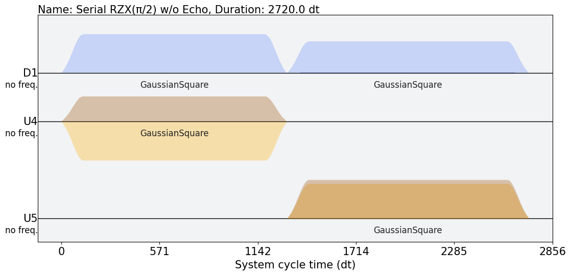
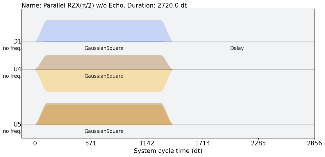
Figure 2: Example pulse sequence for the serial (top) and parallel (bottom) version of the double $R_{ZX}^{\mathrm{\,}}$ gate, as described in LABEL:sec:przx, for the ibmq_belem device. By parallelizing the CR pulses (orange) and merging the compensation tones (blue), the gate duration of two $R_{ZX}^{\mathrm{\,}}$ gates may be reduced by up to half. The parallelization can be made automatically, without additional calibration schemes, by using the $R_{ZX}^{\mathrm{\,}}$ gate pulse shape stemming from the associated CNOT calibration, as described in section III.2.

III.2 Parallel $R_{ZX}^{\mathrm{\,}}$ pulse calibration and design

III.2.1 Pulse calibration from existing $\mathrm{CNOT}$ gates

As the CNOT gate (with echo, see LABEL:app:echo_implementation) is widely used as a standard for 2-qubit entangling quantum gates, the calibration of current quantum devices generally attempts to mitigate the error present in CNOT gate applications. Since the echoed CNOT gates are implemented through the use of cross-resonance (CR) pulses with angle $\theta=\pm\pi/4$, pulses of this format are expected to present lower error rates, and can be used to define suitable pulses for other angle values.

Often, the echoed CNOT gate implementation is achieved by first decomposing the gates in terms of $R_{ZX}(\pi/4)$ (or $R_{ZX}(\pi/2)$ without echo) gates and additional single qubit gates. The error of the CNOT gates is then minimized by calibrating the pulses of the constituting gates, according to the decomposition used. There are several equivalent ways of decomposing CNOT gates in this manner. A possible decomposition for the unechoed CNOT gate is

(20)

(21)

(22)

which is the one often used on IBM’s quantum devices. An alternative formulation is &1@.[