Charge-4e Superconductivity in a Hubbard model

Abstract

A phase of matter in which fermion quartets form a superconducting condensate, rather than the paradigmatic Cooper pairs, is a recurrent subject of experimental and theoretical studies. However, a comprehensive microscopic understanding of charge-4$e$ superconductivity as a quantum phase is lacking. Here, we propose and study a two-orbital tight-binding model with attractive Hubbard-type interactions. Such a model naturally provides the Bose-Einstein condensate as a limit for electron quartets and supports charge-4$e$ superconductivity, as we show by mapping it to a spin-1/2 chain in this perturbative limit. Using both exact diagonalization and density matrix renormalization group calculations for the one-dimensional case, we further establish that the ground state is indeed a superfluid phase of 4$e$ charge carriers and that this phase can be stabilized well beyond the perturbative regime. Importantly, we demonstrate that 4$e$ condensation dominates over 2$e$ condensation even for nearly decoupled orbitals, a scenario suitable for experiments with ultracold atoms in the form of almost decoupled chains. Our model paves the way for both experimental and theoretical exploration of 4$e$ superconductivity and provides a natural starting point for future studies beyond one dimension or more intricate 4$e$ states.

Introduction

Electron pairing is the generic instability of a Fermi liquid in the presence of attractive interactions [1]. This result prompts the question whether superconductivity based on four-electron condensates could exist in physical systems or whether such a phase will always be pre-empted by two-electron superconductivity. Experimentally, definite evidence for charge-4e superconductivity is to date missing. Yet, unusual flux quantization in kagome metals were interpreted as signatures of 4$e$ superconductivity [2, 3, 4], and the breaking of time-reversal symmetry (TRS) above $T_{\rm c}$ in some iron-based superconductors was argued to be compatible with fermion quadrupling [5, 6, 7], although without establishing phase-coherent superconductivity.

Still, several theoretical studies proposed specific scenarios or broader mechanisms that would enable 4e-superconducting phases. These include the thermal fluctuation regime above a pair-density-wave phase, in which 4e-superconductivity appears as a vestigial order [8, 9, 10, 11, 12], doping an antiferromagnet [13], the coupling of two superconducting condensates [14, 15], by frustrating the superconductivity in 45 degree twisted bilayer cuprates [16], through condensation of Skyrmions in a quantum spin-Hall phase [17]. Other attempts have tackled models built as mean-field analogues of Bardeen–Cooper–Schrieffer (BCS) theory for a $4e$ order parameter [18, 19], or by studying a $4e$ analogue of a BCS wavefunction [20] corresponding to a highly non-local Hamiltonian. Despite this plethora of proposals, a microscopic understanding of the quantum nature of 4$e$ superconductivity is missing. A major road block is the lack of a well-behaved microscopic model system amenable to numerical techniques.

In this work, we propose charge-$4e$ superconductivity in an attractive Hubbard-type model, which is local and appeals through its simplicity. The attractive Hubbard model has been a vital theoretical test bed for establishing superconductivity beyond the BCS mean-field approximation [21]. As such, it allows to explore the cross-over from BCS to a Bose-Einstein-condensate (BEC) regime [22, 23, 24] and the competition between charge density wave (CDW) order and singlet superconductivity. The BEC limit of the Hubbard model is a particularly natural starting point: For large enough attractive interactions and no hopping between the sites, fermions are bound into pairs at each lattice site. Adding hopping between the sites as a perturbation then allows the pairs to hop and establish phase coherence at low enough temperatures for appropriate fillings [25]. This physics is well described through mapping the effective low energy model to a hard-core boson or spin model [26]. Here, we generalize the idea of the BEC limit as a starting point by considering two orbitals per site and choosing the interactions between the states such as to form four-electron bound states.

Note that one-dimensional (1D) superconductors are gapless states, for which correlations decay algebraically as a function of distance. Specifically, we define a 1D 4e superconducting as a state in which four-body correlations decay algebraically, while two- and one-body correlations decay exponentially. As a consequence of the charge carriers being quartets, in other words $e^{*}=4e$, this phase should respond to flux insertion with a flux quantization of a quarter of the flux quantum, $\Phi_{0}/4=h/(4e)$.

Model

It is instructive to first construct the BEC limit for the 4e-superconducting phase. Working in the grand-canonical ensemble, we consider a lattice system with—for now—no tunneling between unit cells, and a (near) degeneracy between ground states which differ in filling by four electrons. To realize this situation, we consider a 1D chain with each site containing two spinful orbitals, labeled by $\ell\in\{1,2\}$ and spin index $\sigma\in\{\uparrow,\downarrow\}$ [Fig. 1(a)]. We further denote by $\hat{c}^{\dagger}_{i,\ell,\sigma}$ ($\hat{c}_{i,\ell,\sigma}$) the creation (annihilation) operator for such an electronic state at the $i$th site. The corresponding density operator is $\hat{n}_{i,\ell,\sigma}=\hat{c}^{\dagger}_{i,\ell,\sigma}\hat{c}_{i,\ell,\sigma}$, and we define $\hat{n}_{i,\ell}=(\hat{n}_{i,\ell,\uparrow}+\hat{n}_{i,\ell,\downarrow})$. The onsite Hamiltonian for the $i$-th site reads

$$\hat{H}_{i}=-\mu\sum_{\ell,\sigma}\hat{n}_{i,\ell,\sigma}+U\sum_{\ell}\hat{n}_{i,\ell,\uparrow}\hat{n}_{i,\ell,\downarrow}+V\hat{n}_{i,1}\hat{n}_{i,2},$$ (1)

where $\mu$ is the chemical potential, and $U$ and $V$ are the Hubbard interaction parameters within the same and between different orbitals, respectively. In the following, we focus on the regime $\mu,\,U,\,V<0$ and express all the parameters in units of $(-\mu)$ for compactness of notation. The onsite Hamiltonian, Eq. (1), is diagonal in the occupation number basis, and the four-fold occupied state has energy

$$E_{4}=2\delta,\quad\delta\equiv 2+U+2V.$$ (2)

By tuning $\delta\ll 1$ and $U\sim V$, the low energy subspace of the single-unit-cell Fock space comprises the empty ($N=0$) and four-fold occupied ($N=4$) states only, while the states with particle numbers $N=1,2,3$ lie at higher energy [Fig. 1(b)]. Note that this energy hierarchy can only be reached if $V\neq 0$. At $V=0$ the two orbitals are fully decoupled, and $N=2$ states become part of the low-energy subspace with the $N=4$ state.

For a finite lattice of size $L$, the (near) degeneracy of zero- and four-electron states at every site leads to an extensive (near) ground-state degeneracy of states with $N=4n$ ($n=0,1,\cdots L$) particles. In a thermodynamically large lattice, the (near) degeneracy occurs at all fillings $0<\nu<1$ . The extensive ground-state degeneracy alone is not sufficient to reach a superconducting state. Thus, the full Hamiltonian we consider is obtained by connecting neighboring sites by spin- and orbital-conserving tunneling terms,

$$\hat{H}=\sum_{i=1}^{L}\hat{H}_{i}-t\sum_{i=1}^{L}\sum_{\ell,\sigma}(\hat{c}^{\dagger}_{i,\ell,\sigma}\hat{c}_{i+1,\ell,\sigma}+\text{h.c.}).$$ (3)

By introducing tunneling between the unit cells, the degeneracy is lifted for finite $L$ and may, in the thermodynamic limit, result in a phase-coherent superconducting condensate whose constituents are electronic quartets [27].

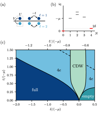
Figure 1: The charge-$4e$ model introduced in Eq. (3): (a) Real-space schematic with a unit cell highlighted by the gray dashed rectangle. (b) Energy levels as a function of particle number $N$ for the single-site Hamiltonian, Eq. (1). (c) Schematic phase diagram as a function of $\delta$, $t$ and $U=V$. The phase boundaries are traced from the iDMRG data obtained at bond dimension $\chi=500$ [28].

Figure. 1(c) shows the ground state phase diagram of Hamiltonian (3) for the SU$(4)$ symmetric [29, 30] case of $U=V$ featuring $4e$ superconductivity in a large part of the parameter space , separated by a ($Q\!=\!\pi$) CDW with filling $\nu=1/2$. While for zero hopping, the system is either empty or full, finite hopping leads to a non-trivial filling and can introduce coherence between sites. Note that this phase diagram can be qualitatively understood, in the limit $t\ll 1$ and $\delta\ll 1$, through a mapping of the low-energy limit to an effective spin-1/2 model, where the two spin states at every site correspond to the empty and four-electron state, namely the quartet of our model, of each site. As compared to the $2e$ case, the hopping of a quartet is a forth-order process, competing with second-order processes, which makes the conclusion about the emergence of a phase-coherent condensate less immediate. Although the effective model has some degree of complexity due to fourth-order terms in perturbation theory, the result simplifies to an XXZ chain with external magnetic field and next-to-nearest neighbor coupling [28]. The effective spin-1/2 model model hosts two fully polarized ferromagnetic phases, which map to the empty and full lattice in the original model, an antiferromagnetic phase, which maps to the fermionic CDW, and a gapless XY phase, which corresponds to the $4e$-superconducting phase. Below, we use exact diagonalization (ED) and density matrix renormalization group (DMRG) to characterize the non-trivial regions of this phase diagram further.

$\pi/2$-periodic magnetic flux response

We first employ ED on a finite chain to gather evidence for a phase-coherent charge-$4e$ superconducting state. The spectrum of a $L=6$ chain with periodic boundary conditions, shown in Fig. 2(a), shows the low-energy modes in the sectors with particle numbers $N=4n$, $n\in\mathbb{Z}_{+}$, and the absolute ground state for $N=16$ particles, which is away from half filling. We further observe a low-lying state at $\nu=1/2$, which we will identify as a charge density wave (CDW) below.

Figure 2(b) depicts the lowest-energy state energy spectrum as a function of flux $\Phi$ through the ring. Conveniently, ED allows to probe the response to such a flux through modification of the tunneling amplitude $t\rightarrow e^{\mathrm{i}\varphi}t$, with $\varphi=2\pi\Phi/(L\Phi_{0})$ with $\Phi_{0}=h/e$ the flux quantum. The spectrum shows two minima with period $\pi/2$, hinting at a $\Phi_{0}/4$ periodicity under flux insertion, the telltale signature of the charge-$4e$ superconducting phase. (Note that we attribute the absence of exact degeneracy of states at $\varphi=0,\,\pi/2,\,\pi,\,3\pi/2$ to finite-size effects.) Importantly, the finite curvature of the spectrum close to $\varphi=0$ is a measure for the non-zero superfluid weight, which is indicative of a coherent state [33, 34, 35, 36, 37].

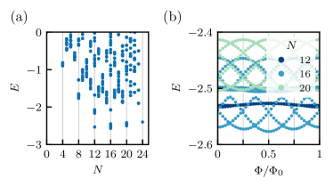
Figure 2: (a) ED spectrum on the $L=6$ chain with periodic boundary conditions for different particle numbers $N$. (b) ED spectrum on the $L=6$ ring as a function of inserted flux $\Phi$. Colors distinguish between states with different particle numbers. For both panels, we use $\delta=-0.2$, $t=0.35$, and $V=U$.

Phase diagram

To combat finite size effects, we next compute the ground state of the model defined in Eq. (3) and its properties using a two-site infinite DMRG (iDMRG) algorithm [38, 39, 40, 41] (see also [28]).

To characterize and distinguish different phases, we define the reduced two- and four-body correlation functions

$$\begin{split}\bar{C}^{(4)}(r)&=C^{(4)}(r)-[C^{(2)}_{\bar{\ell}=0}(r)]^{2},\\ \bar{C}^{(2)}(r)&=C^{(2)}_{\bar{\ell}=0}-[C^{(1)}(r)]^{2},\end{split}$$ (4)

where $C^{(2)}_{\ell,\sigma,\bar{\ell},S}(r)=\absolutevalue{\expectationvalue{\hat{P}^{\dagger}_{0,\ell,\sigma,\bar{\ell},S}\hat{P}_{r,\ell,\sigma,\bar{\ell},S}}}$, $C^{(4)}(r)=\absolutevalue{\expectationvalue{\hat{Q}^{\dagger}_{0}\hat{Q}_{r}}}$, and $C^{(1)}_{\ell,\sigma}(r)=\absolutevalue{\expectationvalue{\hat{c}^{\dagger}_{0,\ell,\sigma}\hat{c}_{r,\ell,\sigma}}}$. All the expectation values are computed over the ground state, and we have introduced the pair and quartet operators

$$\begin{split}\hat{P}_{r,\ell,\sigma,\bar{\ell},S}&=\hat{c}_{r,\ell,\sigma}\hat{c}_{r,\ell+\bar{\ell},\sigma+S},\\ \hat{Q}_{r}&=\hat{c}_{r,1,\uparrow}\hat{c}_{r,1,\downarrow}\hat{c}_{r,2,\uparrow}\hat{c}_{r,2,\downarrow}.\end{split}$$ (5)

We will use the compact notation $\hat{P}_{r,\ell}\equiv\hat{P}_{r,\ell,\uparrow,0,1}=\hat{c}_{r,\ell,\uparrow}\hat{c}_{r,\ell,\downarrow}$ later. The Hamiltonian in Eq. (3) conserves TRS, particle number, and the orbital and spin quantum numbers. Hence, it is sufficient to consider the subset $C^{(2)}_{\bar{\ell}}(r)\equiv C^{(2)}_{1,\uparrow,\bar{\ell},S}(r)$, out of all the two-body correlations, and all the $C^{(1)}_{\ell,\sigma}(r)$’s are equal. In addition, at $U=V$, by SU$(4)$ symmetry, and at $V=0$ the relevant two-body correlation is $C^{(2)}_{\bar{\ell}=0}(r)$ [28]. In Eq. (4) we already used the ensuing simplification by dropping the respective indices.

We now come back to the phase diagram in Fig. 1(c), and explore in detail the physics of the individual phases. In particular, the charge-$4e$ superconducting phase is studied beyond the aforementioned perturbative mapping to a spin-1/2 chain where its existence is rigorously established. At large values of $t$, where a transition to a Luttinger liquid phase occurs, it is suppressed as indicated by the dashed line in Fig. 1(c). Using iDMRG, it is hard to reliably locate this transition between two gapless regimes. Yet, the numerical evidence we discuss below shows the extent of charge-$4e$ superconductivity well beyond the perturbative regime in a substantial portion of the phase diagram.

Figure 3 summarizes the numerical results on three distinct observables, namely the correlations, susceptibilities, and an analysis of operator overlaps with the subleading eigenvectors of the transfer matrix, in three different phases: the charge-4$e$ superconducting phase (upper row), the CDW (central row), and a charge-$2e$ superconducting regime (bottom row) obtained by setting $V=0$.

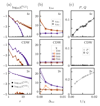
Figure 3: Characterization of the charge-$4e$ (top row), CDW (central row), and charge-$2e$ (bottom row) phases, as obtained from iDMRG. (a) Log-log plot of the absolute value of the correlations in Eq. (4) as a function of distance $r$. (b) Susceptibility to charge-$4e$ and charge-$2e$ perturbations, see Eq. (6). In (a) and (b), markers and colors distinguish types of correlations and susceptibility, respectively, while the opacity indicates the bond dimension $\chi$. (c) $P$ (circles) and $Q$ (squares) transfer matrix overlaps as a function of inverse $\chi$. The (c) bottom panel is evaluated on the charge-2$e$ model. The parameters are $\delta=-0.5,\,t=0.6,\,V/U=1$ (top row), $\delta=0,\,t=1,\,V/U=1$ (central row) and $\delta=-0.3,\,t=0.5,\,V=0$ (bottom row) [28].

Figure 3(a) shows the correlations, Eq. (4), evaluated on the ground state as a function of distance $r$ and different bond dimension $\chi$ of the matrix-product ansatz. In the $4e$-superconducting phase, the two-body correlations decay exponentially for any $\chi$, while the four-body correlations decay algebraically before leveling off at a distance that increases with $\chi$. This constant behavior is an artifact of the finite $\chi$ [42], and an intrinsic limitation of matrix-product states to capture gapless systems [43]. For the CDW case, both correlations decay exponentially. At $V/U=0$, the charge-$2e$ superconducting phase has $\bar{C}^{(2)}$ correlations following an algebraic decay, while $\bar{C}^{(4)}$ is exponentially suppressed.

Figure 3(b) shows the susceptibilities to the charge-$4e$ and charge-$2e$ superconducting perturbations for the same choices of parameters. In particular, we study the susceptibilities to mean-field perturbations of charge-2e and -4e type with perturbations of the form $\delta\hat{H}_{2e}=\Delta_{2e}\sum_{i,\ell}\hat{P}^{\dagger}_{i,\ell}+\text{h.c.}$ and $\delta\hat{H}_{4e}=\Delta_{4e}\sum_{i}\hat{Q}^{\dagger}_{i}+\text{h.c.}$, respectively. These perturbations lead to non-vanishing expectation values $\Delta_{P}=\expectationvalue{\hat{P}^{\dagger}_{1}+\hat{P}^{\dagger}_{2}}$ and $\Delta_{Q}=\expectationvalue{\hat{Q}^{\dagger}}$ with respect to the ground state of the perturbed Hamiltonian, where we dropped the index $r$ due to translational symmetry. Finally, we obtain the susceptibilities

$$\chi_{2e}=\left.\partialderivative{\Delta_{P}}{\Delta_{2e}}\right\rvert_{\Delta_{4e}=0},\quad\chi_{4e}=\left.\partialderivative{\Delta_{Q}}{\Delta_{4e}}\right\rvert_{\Delta_{2e}=0}.$$ (6)

While the exact order parameters for the charge-2$e$ and charge-4$e$ superconductors are in principle not known, we expect a non-zero overlap with $\Delta_{P}$ and $\Delta_{Q}$, respectively. Importantly, for a choice of parameters falling in the charge-$4e$ phase $\chi_{4e}$ shows a peak for $\Delta_{4e}\rightarrow 0$, the charge-$2e$ phase has a peak in $\chi_{2e}$, while the susceptibilities are constant in the CDW phase.

In Fig. 3(c), we analyze more directly the transfer matrix $T$ constructed from the matrix-product ground states in the respective phases [28, 44, 45]. By construction, the largest eigenvalue of $T$ is 1. If the subleading eigenvalue is separated from 1 by a gap that persists in the limit $\chi\to\infty$, all correlations decay exponentially over large enough distances. Indeed, the subleading eigenvalue extrapolates to 1 in this limit in the putative charge-$2e$ and charge-$4e$ phases, while this is not the case in the CDW phase [28]. This allows in principle for algebraic decay of correlations in the former two phases. To deduce which correlations decay algebraically, we compute the overlap between the eigenvector with subleading eigenvalue of $T$ and the pair and quartet operators $\hat{P}^{\dagger}_{1}$ and $\hat{Q}^{\dagger}$, indicated by $P$ and $Q$, respectively [Fig. 3(c)]. While $P$ overlaps dominates in the charge-$2e$ superconducting phase as expected, we observe that $Q$ overlaps dominate in the charge-$4e$ phase.

Stability of charge-$4e$ phase

So far, we have focused on the limits $V=U$ and $V=0$ to establish that they realize, respectively, charge-$4e$ and charge-$2e$ superconducting phases. We now address the interpolating regime $0<V<U$, while keeping $\delta$ constant. Figure 4(a) shows the correlations introduced in Eq. (4). While $\bar{C}^{(4)}$ remains algebraic for any $V<0$, $\bar{C}^{(2)}$ switches from an exponential decay to algebraic at $V/U=0$, suggesting a $4e$ phase for any nonzero $V$. We parametrize the long-distance behavior of the correlations as

$$\bar{C}^{(i)}(r)\sim r^{-\eta_{i}},\quad\bar{C}^{(i)}(r)\sim e^{-\frac{r}{\xi_{i}}},$$ (7)

for algebraic and exponential decay, respectively. While the matrix-product ground state cannot fully capture an algebraic decay [43], we extrapolate the value of $\eta_{i}$’s by considering the correlations up to a finite distance, after which they become constant. In Fig. 4(b), the extracted $\xi_{2},\,\eta_{2}$ for $V/U>0$, and $\eta_{1}$ for $V/U=0$ are shown. Remarkably, the charge-$4e$ phase remains stable over a large parameter range away from $V=U$. Defining a phase boundary between the charge-$4e$ and charge-$2e$ phases is challenging, but our data suggests it lies close to or at $V/U=0$.

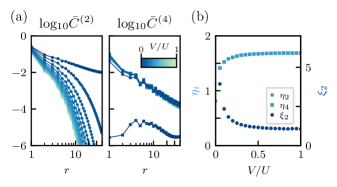
Figure 4: (a) Log-log plot of the correlations defined in Eq. (4) for varying $V/U\in[0,1]$, constant $\delta=0.3$ and $t=0.5$, and at fixed bond dimension $\chi=500$. (b) Exponents extracted from the curves in (a), as defined in Eq. (7).

Discussion

The attractive fermionic Hubbard model describes a system, where a (charge-$2e$) superconducting ground state is unambiguously established theoretically. Realizing superconductivity in the attractive Hubbard model is the declared and realistic goal of cold-atom research [46]. In our work, we have shown that the two-orbital extension of this model realizes a charge-$4e$ superconducting phase at intermediate and strong coupling in a substantial part of its phase diagram. In particular, we found the phase to persist for weak (attractive) interorbital interactions, which addresses the probably biggest limitation in realizing it with cold atoms in experiments.

In addition to the implementation in cold-atom experiments, several theoretical avenues for extending our work present themselves: The approach to construct a charge-$4e$ superconductor can be replicated in higher dimensions. Specifically in two dimensions, the physics of Mott and charge transfer insulators recently described in van der Waals heterostructures may be exploited towards a solid-state experimental realization. Furthermore, the charge-$4e$ order parameter realized in our model transforms trivially under all point group (or internal) symmetries of and can thus be denoted conventional, paralleling the classification of charge-$2e$ superconductors. Exploring unconventional charge-$4e$ superconductors, in other words those that transform as a nontrivial representation of the point group, could lead to the discovery of new topological states.

Acknowledgments

The authors acknowledge useful discussions with Bartholomew Andrews, Edwin Miles Stoudenmire, Johannes Motruk, Martin Zwierlein, Jörg Schmalian, and Daniele Guerci. The authors also acknowledge Nikita Astrakhantsev for his contributions to some of the preliminary calculations of this work. We acknowledge the use of the software packages QuSpin [47, 48] for ED calculations, TeNPy [49] for the iDMRG numerical simulations, and Pymablock [50] to aid the low energy effective model derivation. MOS acknowledges funding from the Forschungskredit of the University of Zurich (Grant number FK-23-110). TN acknowledges support from the Swiss National Science Foundation through a Consolidator Grant (iTQC, TMCG-2_213805).

Supplementary Material

I Charge-2e model

In the main text, we presented a charge-$4e$ model built from a Bose-Einstein-condensate limit, Eq. (3). In this section, we discuss the analogous construction for a charge-$2e$ system. We introduce the 2$e$ model by considering a one-dimensional (1D) chain with a single spinful orbital per site, with $\hat{c}^{\dagger}_{i,\sigma}$ ($\hat{c}_{i,\sigma}$) the creation (annihilation) operator of the electron with spin $\sigma\in\{\uparrow,\downarrow\}$ at the $i$th site. The Hamiltonian for the charge-$2e$ model is the 1D Hubbard model,

$$\hat{H}_{2e}=\sum_{i}\hat{H}_{i}-t\sum_{i,\sigma}\hat{c}^{\dagger}_{i,\sigma}\hat{c}_{i+1,\sigma},\quad\hat{H}_{i}=-\mu\sum_{\sigma}\hat{n}_{i,\sigma}+U\hat{n}_{i,\uparrow}\hat{n}_{i,\downarrow},$$ (S1)

The Hamiltonian for an individual site, $\hat{H}_{i}$, has a four-dimensional Hilbert space, and the two-fold occupied state has energy $\delta\equiv(-2\mu+U)$. For $-\mu<0$, $U<0$ and $\delta\ll 1$, the low energy subspace is made of the empty and two-fold occupied state (Fig. S1(a)). As in the main text, we express the parameters in units of $(-\mu)$ in the following, unless otherwise specified. The hopping term in Eq. (S1) induces coherence between sites and leads to superfluidity in the thermodynamic limit, for the right choices of $\delta,\,t$. The ground-state filling evaluated within ED  is shown in Fig. S1(b), for a chain of length $L=6$. The figure shows two regions where the ground state is the empty or full lattice, a charge density wave (CDW) region, where the ground state is at half filling, and intermediate regions, where the filling interpolates between $0$ or $1$ and $0.5$. Note that in the thermodynamic limit the CDW and the $2e$ gapless phases become degenerate at half filling, and the distinction in Fig. S1(b) is an artifact of finite size effects in ED. Figure S1(c) shows the response of the energy spectrum under flux insertion, which has minima at $\Phi/\Phi_{0}=0,\,\frac{1}{2}$, as expected from a charge-$2e$ superconductor.

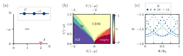
Figure S1: Charge-2e model (a) Energy levels for the single site Hamiltonian, with $\delta=-2\mu+U$. The inset shows the schematic chain structure. (b) Filling of the ground state as a function of $\delta$ and $t$ as obtained from ED on a chain of length $L=6$. (c) Response of the energy spectrum under flux insertion for a chain of length $L=6$, with $\delta=-0.25$ and $t=0.3$.

II Effective spin model in one-dimension

In this section, we outline the derivation of the low energy effective spin-1/2 model for the charge-$4e$ model introduced in the main text, Eq. (3), and we show the resulting phase diagram.

At every site, the local Hilbert space of the full fermionic model Eq. (3) is 16-dimensional. In the low energy effective model we only retain the two lowest-energy states, namely the vacuum and the four-fold occupied state

$$\ket{0},\quad\hat{c}^{\dagger}_{i,1,\uparrow}\hat{c}^{\dagger}_{i,1,\downarrow}\hat{c}^{\dagger}_{i,2,\uparrow}\hat{c}^{\dagger}_{i,2,\downarrow}\ket{0}=\ket{4},$$ (S2)

and integrate out all the remaining states. In the following, we consider $U=V$ for simplicity, and the limit $\delta\ll-\mu$, where the low energy theory is valid. Note that for clarity, in this section we do not express parameters in units of $-\mu$. We take the hopping term of the Hamiltonian in (3) to be the perturbation, with $t\ll-\mu$. For the perturbation theory, we consider terms up to fourth order in $t/(-\mu)$, as this is the minimal order of the perturbative expansion that allows to describe hopping processes of quartets, and we only retain terms to first order in $\delta/(-\mu)$.

In the following, we consider one, two and three sites processes, and we write their contributions to the perturbation theory . There are no corrections coming from four site processes up to this order in perturbation theory.

The Hamiltonian projected on a single site does not contain corrections coming from the tunneling term, but it has only the diagonal entries

$$\bra{0}H\ket{0}=0,\ \bra{4}\hat{H}\ket{4}=2\delta.$$ (S3a)

Considering two sites, we have

$$\begin{split}\bra{0,4}\hat{H}_{t}\ket{0,4}&=-\frac{2t^{2}}{-\mu}\left(1+\frac{\delta}{-2\mu}\right)-\frac{1}{4}\frac{t^{4}}{-\mu^{3}}+O\left(\frac{t^{5}}{\mu^{4}},\frac{\delta^{2}}{-\mu}\right),\\ \bra{0,4}\hat{H}_{t}\ket{4,0}&=-\frac{9}{4}\frac{t^{4}}{-\mu^{3}}+O\left(\frac{t^{5}}{\mu^{4}}\right).\end{split}$$ (S3b)

There are also three-site processes that lead to additional diagonal terms

$$\begin{split}\bra{4,0,0}\hat{H}_{t}\ket{4,0,0}-\bra{4,0}\hat{H}_{t}\ket{4,0}=\bra{4,4,0}\hat{H}_{t}\ket{4,4,0}-\bra{4,0}\hat{H}_{t}\ket{4,0}&=\frac{1}{2}\frac{t^{4}}{\mu^{3}}+O\left(\frac{t^{5}}{\mu^{4}}\right),\\ \bra{0,4,0}\hat{H}_{t}\ket{0,4,0}-2\bra{4,0}\hat{H}_{t}\ket{4,0}=\bra{4,0,4}\hat{H}_{t}\ket{4,0,4}-2\bra{4,0}\hat{H}_{t}\ket{4,0}&=-\frac{2}{5}\frac{t^{4}}{\mu^{3}}+O\left(\frac{t^{5}}{\mu^{4}}\right),\\ \end{split}$$ (S3c)

where we subtract the two-site terms to isolate the contributions from the three-site configurations alone.

The problem can be mapped to a hardcore bosonic model, where we identify

$$\hat{b}^{\dagger}_{i}\equiv\hat{c}^{\dagger}_{i,1,\uparrow}\hat{c}^{\dagger}_{i,1,\downarrow}\hat{c}^{\dagger}_{i,2,\uparrow}\hat{c}^{\dagger}_{i,2,\downarrow},$$ (S4)

and the bosonic operators satisfy the hard-core bosonic algebra

$$[\hat{b}_{i},\hat{b}^{\dagger}_{j}]=\delta_{i,j}(1-2\hat{b}^{\dagger}_{i}\hat{b}_{i}),\quad[\hat{b}_{i},\hat{b}_{j}]=0.$$ (S5)

By collecting all the contributions derived in Eqs. (S3), the effective hard-core bosonic Hamiltonian becomes

$$\begin{split}\hat{H}_{\mathrm{h.c.b.}}=&\frac{9}{4}\frac{t^{4}}{\mu^{3}}\sum_{j}(\hat{b}^{\dagger}_{j}\hat{b}_{j+1}+\text{h.c.})+2\left[\frac{2t^{2}}{\mu}\left(1-\frac{\delta}{2\mu}\right)+\frac{11}{20}\frac{t^{4}}{\mu^{3}}+\delta\right]\sum_{j}\hat{n}_{j}\\ &\quad-2\left[\frac{2t^{2}}{\mu}\left(1-\frac{\delta}{2\mu}\right)-\frac{3}{20}\frac{t^{4}}{\mu^{3}}\right]\sum_{j}\hat{n}_{j}\hat{n}_{j+1}-\frac{7}{5}\frac{t^{4}}{\mu^{3}}\sum_{i}\hat{n}_{i}\hat{n}_{i+2}.\end{split}$$ (S6)

The hard-core bosons can be expressed in terms of spin-1/2 operators $S^{k}_{j}=\sigma^{k}_{j}/2$ ($k=0,1,2,3$, $\sigma^{i}$ Pauli matrices) acting on site $j$

$$\hat{b}^{\dagger}_{i}=2S^{+}_{i}=(S^{x}_{i}+\mathrm{i}S^{y}_{i}),\quad\hat{b}_{i}=2S^{-}_{i}=(S^{x}_{i}-\mathrm{i}S^{y}_{i}),\quad\hat{b}^{\dagger}_{i}\hat{b}_{i}=\hat{n}_{i}=\left(S^{z}_{i}+\frac{\mathbb{1}}{2}\right),$$ (S7)

which satisfy the relations

$$[S^{-}_{i},S^{+}_{j}]=-2\delta_{ij}S^{z}_{i},\quad(\sigma^{\pm}_{i})^{2}=0,\quad S^{x}_{i}S^{x}_{i+1}+S^{y}_{i}S^{y}_{i+1}=2(S^{+}_{i}S^{-}_{i+1}+S^{-}_{i}S^{+}_{i+1}).$$ (S8)

In terms of spin operators, the low energy effective Hamiltonian becomes

$$\begin{split}\hat{H}_{\mathrm{spin}}=&\sum_{i}J(\hat{S}^{x}_{i}\hat{S}^{x}_{i+1}+\hat{S}^{y}_{i}\hat{S}^{y}_{i+1}+\Delta\hat{S}^{z}_{i}\hat{S}^{z}_{i+1})+h\sum_{i}\hat{S}^{z}_{i}+K\sum_{i}\hat{S}^{z}_{i}\hat{S}^{z}_{i+2},\end{split}$$ (S9a)

with the coefficients

$$\begin{split}&J=\frac{9}{4}\frac{t^{4}}{\mu^{3}},\\ &J\Delta=-2\left[\frac{2t^{2}}{\mu}\left(1-\frac{\delta}{2\mu}\right)-\frac{3}{20}\frac{t^{4}}{\mu^{3}}\right],\\ &K=-\frac{7}{5}\frac{t^{4}}{\mu^{3}},\\ &h=2\left[\frac{2t^{2}}{\mu}\left(1-\frac{\delta}{2\mu}\right)+\frac{11}{20}\frac{t^{4}}{\mu^{3}}+\delta\right]+J\Delta+K.\end{split}$$ (S9b)

The resulting low-energy effective model is a non-frustrated XXZ spin-1/2 chain with magnetic field and next-to-nearest-neighbor coupling. Without next-to-nearest-neighbor coupling, meaning $K=0$, this model realizes the paradigmatic XXZ model, which is known to host a paramagnetic gapless superfluid phase [51]. Equivalently, the one-dimensional attractive Hubbard model for hardcore bosons, Eq. (S6), is also known to host a superfluid phase [42].

We compute the ground state of the model in Eq. (S9) within two-site iDMRG, as a function of the perturbative parameters $t/(-\mu)$ and $\delta/(-\mu)$. In Fig. S2, the resulting values for the expectation value of the average $z$-component of the spin $\expectationvalue{S_{z}}$ [Fig S2(a)], its variance var$\expectationvalue{S_{z}}$ [Fig S2(b)], and the spin-spin correlations $\expectationvalue{S^{z}_{0}S^{z}_{r}}-\expectationvalue{S^{z}_{0}}\expectationvalue{S^{z}_{r}}$ [Fig S2(c)], are shown for fixed bond dimension $\chi=50$ and with a maximal energy error cutoff of $10^{-4}$ (see iDMRG parameters section). From these values, we can identify different phases: At small $t/(-\mu)$ and large $\absolutevalue{\delta}/(-\mu)$, the ground state is ferromagnetic ($\expectationvalue{S^{z}}=\pm 0.5$), around $\delta/(-\mu)\sim 0$ the system orders antiferromagnetically ($\expectationvalue{S^{z}}=0$), and for intermediate values there is a superfluid gapless phase ($0<\absolutevalue{\expectationvalue{S^{z}}}<0.5$). In the language of the original fermionic model, the ferromagnetic phases with opposite polarization correspond to a completely empty or completely filled chain, the antiferromagnetic phase maps to a $Q=\pi$ CDW order, where sites are alternatively empty or four-fold occupied, and the gapless superfluid phase translates into a charge-$4e$ superconducting gapless phase.

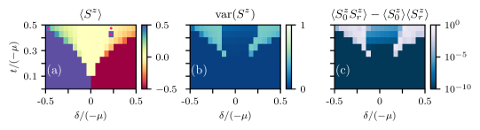
Figure S2: Effective spin model. (a) Expectation value of the $z$-component of the spin $S^{z}$, (b) its variance, and (c) correlations measured at a fixed distance $r=10$. These values are obtained within iDMRG with bond dimension $\chi=50$. Data points marked by a pink dot in (a) correspond to iDMRG runs that reached the maximal number of sweeps before reaching the accuracy $\Delta E$.

III iDMRG

III.1 iDMRG parameters

The iDMRG results presented throughout this work have been obtained by using the two-site iDMRG algorithm implemented in the TeNPy library (version 0.10.0) [49]. The main parameters for the iDMRG runs used throughout this work are

• "chi_list": {0:$\chi/2$, n_1:$3\chi/4$, n_2:$\chi$}, where $\chi$ is the bond dimension quoted with the data. The values n_1 and n_2 are of order 20 and 50, respectively.

• "trunc_params":{"svd_min":1.e-15, "trunc_cut":1e-8}, and "update_env":10.

• "max_E_err"="max_S_err"=$\Delta E$. The parameter $\Delta E$, determines the two-site iDMRG convergence threshold, and we take the same for both energy and entropy convergence. Generically, $\Delta E$ is taken in the range $10^{-4}$–$10^{-8}$, depending on the phase and model.

• "min_sweeps": 50, and "max_sweeps": between 500 and 1000,

• "mixer":True, with parameters:

  "mixer_params":{"amplitude":1.e-5, "decay":1.2, "disable_after":30}

The remaining parameters are set to the TeNPy default.

III.2 Phase diagram from iDMRG

In this section, we present in more detail the numerical results obtained within iDMRG applied to the model of Eq. (3) in the main text, in other words, the full fermionic model that realizes a charge-4e superconducting phase. To characterize the phase boundaries, we obtain a series of observables evaluated on the iDMRG ground state: the results are collected in Fig. S3 at bond dimension $\chi=500$, $\Delta E=10^{-6}$. The quantities shown in the panels of Fig. S3 are defined as follows:

1. Filling: $\nu=\sum_{i,\ell,\sigma}\expectationvalue{\hat{n}_{i,\sigma,\ell}}_{\mathrm{GS}}/8$, where $i$ runs over the two sites over which the iDMRG minimization is performed, and $\ell$ and $\sigma$ are the orbital and spin index respectively.

2. Variance of the filling: $\text{var}(\nu)=\frac{1}{16}\sum_{i,\ell,\sigma}\expectationvalue{\hat{n}^{2}_{i,\sigma,\ell}}_{\mathrm{GS}}-\nu^{2}$.

3. The CDW order parameter is $O_{\text{CDW}}=\frac{1}{16}\sum_{i,j}(-1)^{i+j}N_{i}N_{j}$, where $N_{i}=\sum_{\ell,\sigma}\expectationvalue{\hat{n}_{i,\ell,\sigma}}_{\mathrm{GS}}$.

4. The correlations $C^{(1)}$, $\bar{C}^{(2)}$ and $\bar{C}^{(4)}$ are the ones introduced in the main text, for the SU(4) symmetric case.

The jumps in the values of the filling, correlations and the CDW order parameters then allow us to trace the phase boundaries sketched in Fig. 1 of the main text. The transitions between empty and full lattice towards the gapless charge-$4e$ phase is sharply defined by the jump in the value of $\nu$ as well as the correlations, and the same holds for the transition between CDW and charge-$4e$ phase. The phase boundaries that separates the charge-$4e$ phase and the CDW from the Luttinger liquid are less sharp, and therefore harder to numerically pinpoint.

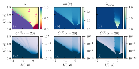
Figure S3: Charge-4e model. iDMRG data evaluated at constant bond dimension $\chi=500$, and maximal energy error $1e-6$, as a function of $t$ and $\delta$. Pink dots indicate data points for which the iDMRG run reached the maximal number of sweeps. The panels display the following quantities evaluated on the ground state: (a) Filling, (b) variance of the filling, (c) order paramter for the CDW, (d)–(f) correlations at a fixed distance $r=10$, respectively (d) $C^{(1)}$, (e) $\bar{C}^{(2)}$, and (f) $\bar{C}^{(4)}$. Note that for (d)–(f) the colorscale is logaritmic, hence correlations below the value $10^{-12}$ are flattened.

Figure S4 shows the behavior of the $\bar{C}^{(4)}$ correlations across two phase transitions: between the fully-filled ground state and the $4e$ phases, and between the $4e$ and CDW phases, for different choices of bond dimension $\chi$. The figure suggests that the results are converged to a sufficient degree for $\chi=500$ and thus, showcases how the choice of $\chi=500$ for the phase diagram allows to trace the same boundaries that would be obtained at higher values of $\chi$, within sufficient accuracy, while being more accessible numerically.

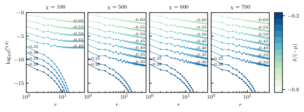
Figure S4: Bond dimension scaling. Log-log fountain plot of $\bar{C}^{(4)}(r)$ correlations for different bond dimension $\chi$ (specified by the panel titles). The correlations are evaluated within two-site iDMRG, with $\Delta E=10^{-6}$, at fixed $t/(-\mu)=0.6$ and varying $\delta/(-\mu)\in[-0.8,-0.2]$. For each value of $\delta$, correlations are shifted by an equally spaced offset, for visibility, and different values of $\delta$ are both labeled by the corresponding value and distinguished by color. In the phase with ground state filling $\nu=1$, correlations are constant and zero, therefore they do not appear in the panels. This choice of parameters drives the system across two phase boundaries: first between the full lattice ($\delta\leq-0.65$) and the $4e$ phase ($\delta\geq-0.60$), and then between $4e$ ($\delta\leq-0.30$) and the CDW ($\delta\geq-0.35$) phases. Dashed lines indicate that the iDMRG calculation reached the maximal number of sweeps before reaching the energy precision, which occurs close to the phase boundaries values.

For completeness, in Fig. S5 we show all the bare (without subtraction) correlations for the same choices of model parameters of Fig. 3 in the main text. In the SU(4) symmetric cases [Fig. S5(a), (b)], the ${C^{(2)}_{\bar{\ell}}}$’s are equal, while for $V=0$ [Fig. S5(c)] only ${C^{(2)}_{\bar{\ell}=0}}$ displays algebraic decay, while ${C^{(2)}_{\bar{\ell}=1}}$ decays exponentially. For this, in the main text we only display ${C^{(2)}_{\bar{\ell}=0}}$ as it suffices to characterize the phases.

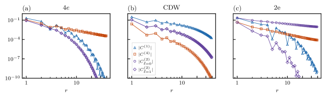
Figure S5: Bare correlations Log-log plot of the bare correlations evaluated on the ground state of the model in Eq. (3), for (a) the $4e$ phase, (b) the CDW, and (c) the $2e$ phase. The panels correspond to the same choice of model parameters of Fig. 3 in the main text: (a) $\delta=-0.5,\,t=0.6,\,V/U=1$, (b) $\delta=0,\,t=1,\,V/U=1$, and (c) $\delta=-0.3,\,t=0.5,\,V=0$. Here all correlations are obtained at fixed bond dimension $\chi=700$.

III.3 Transfer matrix overlaps

To further characterize and distinguish the charge-$4e$ phase from a $2e$-superconducting state, we compare the overlaps of some relevant operators with the second leading eigenvalue of the transfer matrix obtained from the iDMRG ground state.

The charge-$4e$ and the charge-$2e$ superconducting phases are gapless, and this manifests in the divergence of the correlation length $\xi$ as a function of bond dimension $\chi$. The correlation length, in turn, is extracted from the second leading eigenvalue of the transfer matrix $\lambda_{2}$, through the relation $\lambda_{2}=e^{-\frac{1}{\xi}}$. In other words, the gaplessness of the phase also manifests as $\lambda_{2}(\chi)\rightarrow 1$ as $\chi\rightarrow\infty$ (where we write $\lambda_{2}(\chi)$ to make the dependence on $\chi$ explicit).

Let us consider connected correlators of the following form, for a translationally invariant system

$$C_{O}(|i-j|)=\expectationvalue{\hat{O}^{\dagger}_{i}\hat{O}_{j}}_{\mathrm{GS}}-\expectationvalue{\hat{O}^{\dagger}_{i}}_{\mathrm{GS}}\expectationvalue{\hat{O}_{j}}_{\mathrm{GS}},$$ (S10)

where $\hat{O}_{i}$ is an operator acting on site $i$. These can be expressed as [45]

$$C_{O}(|i-j|)=\tr[\hat{O}^{\dagger}_{i}T^{|i-j-1|}\hat{O}_{j}]-\expectationvalue{\hat{O}^{\dagger}_{i}}_{\mathrm{GS}}\expectationvalue{\hat{O}_{j}}_{\mathrm{GS}}$$ (S11)

where $T$ is the transfer matrix. The transfer matrix can be decomposed in terms of its eigenvalues $\{\lambda_{i}\}$ and eigenvectors $v_{i}$ (ordered as $\absolutevalue{\lambda_{1}}>\absolutevalue{\lambda_{2}}\geq\absolutevalue{\lambda_{2}}\geq\cdots\geq\absolutevalue{\lambda_{{\chi^{2}}}}$)

$$T=\sum_{i=1}^{\chi^{2}}\lambda_{i}\ket{v_{i}}\bra{v_{i}}$$ (S12)

with the largest eigenvalue $\lambda_{1}=\max\{\lambda_{i}\}_{i=1}^{\chi^{2}}=1$, and all the other eigenvalues $|\lambda_{i}|<1$ for $i\neq 1$. The connected correlator can then be expressed as

$$C_{O}(|i-j|)=\Big{\langle}\hat{O}^{\dagger}_{i}\left(\sum_{i=2}^{\chi^{2}}\lambda^{|i-j+1|}_{v_{i}}\ket{v_{i}}\bra{v_{i}}\right)\hat{O}_{j}\Big{\rangle}.$$ (S13)

Therefore, maximizing the overlap between the second leading eigenvalue $v_{2}$ and a generic operator $\hat{O}$ conveys which operator is characterized by the slowest exponential decay across the MPS ground state. This, for a gapless phase, would lead to algebraic decay in the limit of $\chi\rightarrow\infty$, combined with the correlation length divergence. In practice, there is a finite number of symmetry inequivalent operators in our model, therefore it is sufficient to evaluate the overlaps for each operator to find the maximal overlap with $v_{2}$. In particular, we consider

$$\begin{split}\hat{P}^{\dagger}_{1}=\hat{c}^{\dagger}_{1,\uparrow}\hat{c}^{\dagger}_{1,\downarrow},\quad\hat{P}^{\dagger}_{1,2}=\hat{c}^{\dagger}_{1,\uparrow}\hat{c}^{\dagger}_{2,\downarrow},\quad\hat{P}^{\dagger\prime}_{1,2}=\hat{c}^{\dagger}_{1,\uparrow}\hat{c}^{\dagger}_{2,\uparrow},\quad\hat{Q}^{\dagger}=\hat{c}^{\dagger}_{1,\uparrow}\hat{c}^{\dagger}_{1,\downarrow}\hat{c}^{\dagger}_{2,\uparrow}\hat{c}^{\dagger}_{2,\downarrow}.\end{split}$$ (S14)

We indicate the overlap of the operator $\hat{O}^{\dagger}_{\alpha}$ with $v_{2}$ by $O_{\alpha}$. In the main text, we only show $P_{1}$, $Q$ and leave out $P_{1,2}$ and $P_{1,2}^{\prime}$ as the two-particle operator overlaps are all equivalent at $U=V$.

The spectra of the transfer matrix, correlation length and the overlaps of the operators are shown in Figs. S6, S7,S8. The charge-$4e$ and CDW cases are evaluated within the charge-$4e$ model of Eq. (3), while the charge-$2e$ phase is evaluated on the single orbital chain, see the model of Eq. (S1)

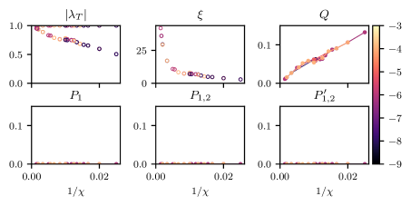
Figure S6: Transfer-matrix analysis in the charge-4e phase. This figure shows some transfer matrix numerical results obtained in the charge-4e model with parameters $\delta=-0.5$, $t=0.6$, and $V/U=1$, as a function of inverse bond dimension $\chi$. Colors indicate the $\log_{10}(\Delta E)$ of the maximal energy error $\Delta E$. The first two panels show the three largest eigenvalues of the transfer matrix spectrum (panel $|\lambda_{T}|$) and the correlation length extracted from $\lambda_{2}$ (panel $\xi$). The remaining panels show the $O_{\alpha}$ overlaps, following the notation introduced in Eq. (S14).

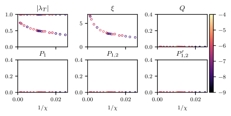
Figure S7: Transfer Matrix in the CDW phase. This figure shows some transfer matrix numerical results obtained in the charge-4e model with parameters $\delta=0$, $t=1$, and $V/U=1$, as a function of inverse bond dimension $\chi$. Colors indicate the $\log_{10}(\Delta E)$ of the maximal energy error $\Delta E$. The first two panels show the three largest eigenvalues of the transfer matrix spectrum (panel $|\lambda_{T}|$) and the correlation length extracted from $\lambda_{2}$ (panel $\xi$). The remaining panels show the $O_{\alpha}$ overlaps, following the notation introduced in Eq. (S14).

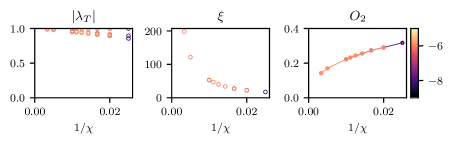
Figure S8: Transfer Matrix in the charge-2e phase. This figure shows some transfer matrix numerical results obtained in the charge-2e model with parameters $\delta=-0.3$, $t=0.5$, as a function of inverse bond dimension $\chi$. Colors indicate the $\log_{10}(\Delta E)$ of the maximal energy error $\Delta E$. The panels show the three largest eigenvalues of the transfer matrix spectrum (panel $|\lambda_{T}|$) and the correlation length extracted from $\lambda_{2}$ (panel $\xi$, and the last panel shows the $O_{2}$ overlaps, following the notation introduced in Eq. (S14).

References

- Cooper [1956] L. N. Cooper, Bound Electron Pairs in a Degenerate Fermi Gas, Phys. Rev. 104, 1189 (1956).
- Ge et al. [2022] J. Ge, P. Wang, Y. Xing, Q. Yin, H. Lei, Z. Wang, and J. Wang, Discovery of charge-4e and charge-6e superconductivity in kagome superconductor CsV3Sb5 (2022), 2201.10352 .
- Pan et al. [2022] Z. Pan, C. Lu, F. Yang, and C. Wu, Frustrated superconductivity and “charge-6e” ordering (2022), arXiv:2209.13745 .
- Zhou and Wang [2022] S. Zhou and Z. Wang, Chern Fermi pocket, topological pair density wave, and charge-4e and charge-6e superconductivity in kagomé superconductors, Nature Communications 13, 10.1038/s41467-022-34832-2 (2022).
- Grinenko et al. [2021] V. Grinenko, D. Weston, F. Caglieris, C. Wuttke, C. Hess, T. Gottschall, I. Maccari, D. Gorbunov, S. Zherlitsyn, J. Wosnitza, A. Rydh, K. Kihou, C.-H. Lee, R. Sarkar, S. Dengre, J. Garaud, A. Charnukha, R. Hühne, K. Nielsch, B. Büchner, H.-H. Klauss, and E. Babaev, State with spontaneously broken time-reversal symmetry above the superconducting phase transition, Nature Physics 17, 1254 (2021).
- Maccari et al. [2023] I. Maccari, J. Carlström, and E. Babaev, Prediction of time-reversal-symmetry breaking fermionic quadrupling condensate in twisted bilayer graphene, Phys. Rev. B 107, 064501 (2023).
- Maccari and Babaev [2022] I. Maccari and E. Babaev, Effects of intercomponent couplings on the appearance of time-reversal symmetry breaking fermion-quadrupling states in two-component london models, Phys. Rev. B 105, 214520 (2022).
- Wu [2005] C. Wu, Competing orders in one-dimensional spin- fermionic systems, Phys. Rev. Lett. 95, 266404 (2005).
- Berg et al. [2009] E. Berg, E. Fradkin, and S. A. Kivelson, Charge-4e superconductivity from pair-density-wave order in certain high-temperature superconductors, Nature Physics 5, 830 (2009), arXiv:0904.1230 .
- Berg et al. [2009] E. Berg, E. Fradkin, and S. A. Kivelson, Theory of the striped superconductor, Phys. Rev. B 79, 064515 (2009).
- Agterberg et al. [2020] D. F. Agterberg, J. S. Davis, S. D. Edkins, E. Fradkin, D. J. Van Harlingen, S. A. Kivelson, P. A. Lee, L. Radzihovsky, J. M. Tranquada, and Y. Wang, The physics of pair-density waves: Cuprate superconductors and beyond, Annual Review of Condensed Matter Physics 11, 231 (2020), https://doi.org/10.1146/annurev-conmatphys-031119-050711 .
- Jian et al. [2021] S.-K. Jian, Y. Huang, and H. Yao, Charge- superconductivity from nematic superconductors in two and three dimensions, Phys. Rev. Lett. 127, 227001 (2021).
- Kivelson et al. [1990] S. A. Kivelson, V. J. Emery, and H. Q. Lin, Doped antiferromagnets in the weak-hopping limit, Phys. Rev. B 42, 6523 (1990).
- Herland et al. [2010] E. V. Herland, E. Babaev, and A. Sudbø, Phase transitions in a three dimensional lattice london superconductor: Metallic superfluid and charge- superconducting states, Phys. Rev. B 82, 134511 (2010).
- Fernandes and Fu [2021] R. M. Fernandes and L. Fu, Charge- Superconductivity from Multicomponent Nematic Pairing: Application to Twisted Bilayer Graphene, Phys. Rev. Lett. 127, 047001 (2021).
- Liu et al. [2023] Y.-B. Liu, J. Zhou, C. Wu, and F. Yang, Charge 4e superconductivity and chiral metal in the -twisted bilayer cuprates and similar materials (2023), arXiv:2301.06357 .
- Moon [2012] E.-G. Moon, Skyrmions with quadratic band touching fermions: A way to achieve charge superconductivity, Phys. Rev. B 85, 245123 (2012).
- Jiang et al. [2017] Y.-F. Jiang, Z.-X. Li, S. A. Kivelson, and H. Yao, Charge- superconductors: A Majorana quantum Monte Carlo study, Phys. Rev. B 95, 241103 (2017).
- Gnezdilov and Wang [2022] N. V. Gnezdilov and Y. Wang, Solvable model for a charge- superconductor, Phys. Rev. B 106, 094508 (2022).
- Li et al. [2022] P. Li, K. Jiang, and J. Hu, Charge 4 superconductor: a wavefunction approach (2022), arXiv:2209.13905 .
- Micnas et al. [1990] R. Micnas, J. Ranninger, and S. Robaszkiewicz, Superconductivity in narrow-band systems with local nonretarded attractive interactions, Rev. Mod. Phys. 62, 113 (1990).
- Robaszkiewicz et al. [1981] S. Robaszkiewicz, R. Micnas, and K. A. Chao, Hartree theory for the negative- extended Hubbard model: Ground state, Phys. Rev. B 24, 4018 (1981).
- Robaszkiewicz et al. [1982] S. Robaszkiewicz, R. Micnas, and K. A. Chao, Hartree theory for the negative- extended Hubbard model. II. Finite temperature, Phys. Rev. B 26, 3915 (1982).
- Nozières and Schmitt-Rink [1985] P. Nozières and S. Schmitt-Rink, Bose condensation in an attractive fermion gas: From weak to strong coupling superconductivity, Journal of Low Temperature Physics 59, 195 (1985).
- Ho et al. [2009] A. F. Ho, M. A. Cazalilla, and T. Giamarchi, Quantum simulation of the Hubbard model: The attractive route, Phys. Rev. A 79, 033620 (2009).
- Singer et al. [1998] J. Singer, T. Schneider, and M. Pedersen, On the phase diagram of the attractive Hubbard model: Crossover and quantum critical phenomena, Eur. Phys. J. B , 17–30 (1998).
- Greiter [2005] M. Greiter, Is electromagnetic gauge invariance spontaneously violated in superconductors?, Annals of Physics 319, 217 (2005).
- [28] Supplementary Material. In the Supplementary Material accompanying this paper we discuss the charge-2 model analogous to the one presented in the main text, and the derivation of the low energy effective spin model of the charge-4 system. We also include additional information on the iDMRG calculations, such as the iDMRG paramters, numerical data for the phase diagram presented in the main text, and a more detailed explanation of how we obtain the transfer matrix overlaps.
- Assaraf et al. [1999] R. Assaraf, P. Azaria, M. Caffarel, and P. Lecheminant, Metal-insulator transition in the one-dimensional Hubbard model, Phys. Rev. B 60, 2299 (1999).
- Honerkamp and Hofstetter [2004] C. Honerkamp and W. Hofstetter, Ultracold Fermions and the Hubbard Model, Phys. Rev. Lett. 92, 170403 (2004).
- Lieb and Wu [1968] E. H. Lieb and F. Y. Wu, Absence of Mott Transition in an Exact Solution of the Short-Range, One-Band Model in One Dimension, Phys. Rev. Lett. 20, 1445 (1968).
- Sólyom [1979] J. Sólyom, The Fermi gas model of one-dimensional conductors, Advances in Physics 28, 201 (1979).
- Kosterlitz and Thouless [1973] J. M. Kosterlitz and D. J. Thouless, Ordering, metastability and phase transitions in two-dimensional systems, Journal of Physics C: Solid State Physics 6, 1181 (1973).
- Nelson and Kosterlitz [1977] D. R. Nelson and J. M. Kosterlitz, Universal jump in the superfluid density of two-dimensional superfluids, Phys. Rev. Lett. 39, 1201 (1977).
- Shastry and Sutherland [1990] B. S. Shastry and B. Sutherland, Twisted boundary conditions and effective mass in Heisenberg-Ising and Hubbard rings, Phys. Rev. Lett. 65, 243 (1990).
- Scalapino et al. [1993] D. J. Scalapino, S. R. White, and S. Zhang, Insulator, metal, or superconductor: The criteria, Phys. Rev. B 47, 7995 (1993).
- Scalapino et al. [1992] D. J. Scalapino, S. R. White, and S. C. Zhang, Superfluid density and the Drude weight of the Hubbard model, Phys. Rev. Lett. 68, 2830 (1992).
- White [1992] S. R. White, Density matrix formulation for quantum renormalization groups, Phys. Rev. Lett. 69, 2863 (1992).
- White [1993] S. R. White, Density-matrix algorithms for quantum renormalization groups, Phys. Rev. B 48, 10345 (1993).
- Schollwöck [2005] U. Schollwöck, The density-matrix renormalization group, Rev. Mod. Phys. 77, 259 (2005).
- McCulloch [2008] I. P. McCulloch, Infinite size density matrix renormalization group, revisited (2008), arXiv:0804.2509 [cond-mat.str-el] .
- Kiely and Mueller [2022] T. G. Kiely and E. J. Mueller, Superfluidity in the one-dimensional Bose-Hubbard model, Phys. Rev. B 105, 134502 (2022).
- Rams et al. [2018] M. M. Rams, P. Czarnik, and L. Cincio, Precise Extrapolation of the Correlation Function Asymptotics in Uniform Tensor Network States with Application to the Bose-Hubbard and XXZ Models, Phys. Rev. X 8, 041033 (2018).
- Haegeman and Verstraete [2017] J. Haegeman and F. Verstraete, Diagonalizing transfer matrices and matrix product operators: A medley of exact and computational methods, Annual Review of Condensed Matter Physics 8, 355 (2017), https://doi.org/10.1146/annurev-conmatphys-031016-025507 .
- Vanderstraeten et al. [2019] L. Vanderstraeten, J. Haegeman, and F. Verstraete, Tangent-space methods for uniform matrix product states, SciPost Phys. Lect. Notes , 7 (2019).
- Hartke et al. [2023] T. Hartke, B. Oreg, C. Turnbaugh, N. Jia, and M. Zwierlein, Direct observation of nonlocal fermion pairing in an attractive Fermi-Hubbard gas, Science 381, 82 (2023).
- Weinberg and Bukov [2017] P. Weinberg and M. Bukov, QuSpin: a Python package for dynamics and exact diagonalisation of quantum many body systems part I: spin chains, SciPost Phys. 2, 003 (2017).
- Weinberg and Bukov [2019] P. Weinberg and M. Bukov, QuSpin: a Python package for dynamics and exact diagonalisation of quantum many body systems. Part II: bosons, fermions and higher spins, SciPost Phys. 7, 020 (2019).
- Hauschild and Pollmann [2018] J. Hauschild and F. Pollmann, Efficient numerical simulations with Tensor Networks: Tensor Network Python (TeNPy), SciPost Phys. Lect. Notes , 5 (2018), code available from https://github.com/tenpy/tenpy, arXiv:1805.00055 .
- Araya Day et al. [2023] I. Araya Day, S. Miles, D. Varjas, and A. R. Akhmerov, Pymablock (2023).
- Franchini [2016] F. Franchini, An Introduction to Integrable Techniques for One-Dimensional Quantum Systems, Vol. 940 (Lecture Notes in Physics, 2016).