^∗Department of Physics, University of Illinois Urbana-Champaign
Urbana, IL 61801

^†PITT PACC, University of Pittsburgh
Pittsburgh, PA, USA

^‡Center for Quantum Mathematics and Physics (QMAP)
University of California, Davis, CA 95616

^♢Department of Physics and Astronomy
University of Utah, Salt Lake City, UT 94103

Interactions between dark matter and ordinary matter will transfer momentum, and therefore give rise to a force on ordinary matter due to the dark matter ‘wind.’ We present a realistic model of dark matter where this force can be maximal, meaning that an order-1 fraction of the dark matter momentum incident on a target of ordinary matter is reflected. The model consists of light ($m_{\phi}\mathrel{{\mathrel{\raise 1.29167pt\hbox{$<$\kern-7.5pt\lower 4.30554pt\hbox{$\sim$}}}}}\text{eV}$) scalar dark matter with an effective interaction $\phi^{2}\bar{\psi}\psi$, where $\psi$ is an electron or nucleon field. If the coupling is repulsive and sufficiently strong, the field $\phi$ is excluded from ordinary matter, analogous to the Meissner effect for photons in a superconductor. We show that there is a large region of parameter space that is compatible with existing constraints, and which can be probed by sensitive force experiments, such as satellite tests of the equivalence principle and torsion balance experiments.

1 Introduction

Understanding the microscopic nature of dark matter is one of the major open problems in particle physics and cosmology. Dark matter has been detected only through its gravitational interactions, but additional interactions are needed in order to explain its relic abundance, giving hope that we can find additional signals of dark matter in the laboratory or astrophysical or cosmological observations. The allowed dark matter masses and interactions span a vast parameter space, and it is important to carry out experimental searches for as wide a range of models as possible.

In this paper, we consider a new probe of dark matter: the force on ordinary matter due to an incident flux of dark matter—the dark matter ‘wind.’ Due to the motion of the stars in the galaxy relative to the dark matter halo, the local dark matter is moving relative to the solar system with an average speed $v_{\text{DM}}\sim 300~{}\text{km}/\text{s}\sim 10^{-3}c$. We can estimate the maximal force that could be exerted by the dark matter wind by assuming that the full flux of dark matter on an object is reflected by the object. If the dark matter interacted strongly with a macroscopic target with cross-sectional area $A$, the force exerted by the dark matter on the target is given by

$$F_{\text{max}}\sim\rho^{\vphantom{2}}_{\text{DM}}v_{\text{DM}}^{2}A,$$ (1.1)

where $\rho_{\text{DM}}\sim 0.3$ GeV$/$cm³ is the dark matter density near the earth. The corresponding acceleration of a solid sphere of radius $R$ and density $\rho$ is

$$a_{\text{max}}\sim 10^{-12}~{}\text{m}/\text{s}^{2}\hskip 1.00006pt\left(\frac{R}{\text{cm}}\right)^{-1}\left(\frac{\rho}{10~{}\text{g}/\text{cm}^{3}}\right)^{-1}.$$ (1.2)

These accelerations are large enough to be detected using sensitive low-frequency force probes, such as those used to test the equivalence principle [1, 2, 3].

The interactions of dark matter with ordinary matter are strongly constrained by direct dark matter searches, as well as cosmological and astrophysical constraints. Nonetheless, we will show that there is a model of dark matter where the force on ordinary matter can be maximal, and which is compatible with all these constraints. In this model, dark matter is described by a light scalar field $\phi$ with an effective coupling

$$\mathcal{L}_{\text{int}}=-\frac{1}{2f_{\psi}}\phi^{2}\bar{\psi}\psi,$$ (1.3)

where $\psi$ is an electron or nucleon field. The absence of a Yukawa coupling $\phi\bar{\psi}\psi$ can be explained by a $\mathbb{Z}_{2}$ symmetry under which $\phi\mapsto-\phi$. In a region containing matter, we have $\langle\bar{\psi}\psi\rangle=n_{\psi}$ in the non-relativistic limit, where $n_{\psi}$ is the number density of $\psi$ particles. Therefore, this interaction gives an additional contribution to the dark matter mass inside matter:

$$\Delta m_{\phi}^{2}=\frac{n_{\psi}}{f_{\psi}}.$$ (1.4)

We will consider the case $f_{\psi}>0$, so that $\Delta m_{\phi}^{2}>0$. Inside matter, the relation between the energy and and momentum of a $\phi$ particle is modified:

$$E_{\text{matt}}=\sqrt{k_{\text{matt}}^{2}+m_{\phi}^{2}+\Delta m_{\phi}^{2}}.$$ (1.5)

If $\Delta m_{\phi}^{2}$ is sufficiently large, then the propagation of dark matter is suppressed inside matter. For a $\phi$ particle in vacuum with momentum $k$ incident on a region of ordinary matter, energy conservation gives

$$E_{\text{matt}}=E_{\text{vac}}=\sqrt{k_{\text{vac}}^{2}+m_{\phi}^{2}},$$ (1.6)

and we see that $k_{\text{matt}}^{2}<0$ for $\Delta m_{\phi}^{2}>k_{\text{vac}}^{2}$. If this is satisfied, then the matter region is classically forbidden, and the propagation of the dark matter is exponentially suppressed. This is a coherent scattering effect that is important when the density of scatterers is large compared to the de Broglie wavelength of the dark matter. It is analogous to the Meissner effect for photons in a superconductor, so we call this the ‘dark matter Meissner effect.’

We will show that there is a large region of the $m_{\phi},f$ parameter space of this model where the dark matter Meissner effect takes place, which are allowed by laboratory and astrophysical/cosmological constraints. This occurs for very light dark matter, $m_{\phi}\mathrel{{\mathrel{\raise 1.29167pt\hbox{$<$\kern-7.5pt\lower 4.30554pt\hbox{$\sim$}}}}}\text{eV}$, where it is a good approximation to treat the dark matter as a coherent classical wave. This opens the exciting possibility that it may be possible to directly measure the force exerted by dark matter on ordinary matter. We emphasize that here we are discussing the average force due to the motion of the dark matter, rather than the oscillatory force due to coherent $\phi$ oscillations with frequency $\omega=m_{\phi}$, which has been previously considered in the literature [4, 5]. We expect the wind force to dominate if we average over time scales longer than the coherence time of these oscillations, which is of order

$$t_{\text{coherence}}\sim\frac{1}{m_{\phi}v_{\text{DM}}^{2}}\sim\text{sec}\left(\frac{m_{\phi}}{10^{-8}\mathrm{~{}eV}}\right)^{-1}.$$ (1.7)

The strong interaction between ordinary matter and dark matter makes the detection of the dark matter wind force possible, but it also means that ordinary matter can act as a shield for the dark matter wind. Because of this shielding effect, we are not able to identify any existing force experiments that are sensitive to this force. We will give estimates for the size of the force, and discuss some possible future experiments that may be sensitive to it. Further work is needed to design an experiment that is sensitive to this force.

This paper is organized as follows. In §2, we discuss the physics of the dark matter Meissner effect. In §3 we review existing constraints on the model. In §4 we give estimates for the size of the force on potential experimental targets. Our conclusions are given in §5. Appendices give additional details of our calculations, and discuss UV completions and fine tuning.

2 The Dark Matter Meissner Effect

In this section we discuss the dark matter Meissner effect in more detail. We begin with some simple estimates for the the parameter regime where the effect takes place and can lead to a maximal force on a target. We then explain the methods used to perform precise calculations of the force, and give some parametric estimates for various limiting cases.

2.1 Estimates

In the presence of matter, coherent scattering effects can be important if the density of scatterers is sufficiently high. For example, for the earth’s atmosphere, we have

$$\frac{\bar{\lambda}_{\text{dB}}}{n_{\text{atm}}^{-1/3}}\sim 10^{5}\left(\frac{m_{\phi}}{\text{eV}}\right)^{-1},$$ (2.1)

where $\bar{\lambda}_{\text{dB}}=1/m_{\phi}v_{\phi}$ is the reduced de Broglie wavelength of the dark matter particles in vacuum and $n_{\text{atm}}$ is the number density of nucleons near the earth’s surface. As long as this ratio is large in the parameter range we are interested in we can approximate the matter as continuous. Inside matter, we then have

$$\langle\bar{\psi}\psi\rangle=n_{\psi}\sim\frac{\rho_{\text{matter}}}{m_{p}},$$ (2.2)

where $n_{\psi}$ is the number density of $\psi$ particles (nucleons or electrons) in matter . Therefore, as discussed in the introduction, dark matter will be excluded from regions of sufficiently high density if $\Delta m_{\phi}^{2}>k_{\text{vac}}^{2}$, where $\Delta m_{\phi}^{2}$ is the matter contribution to the dark matter mass. This condition is satisfied for

$$\frac{1}{f}\mathrel{{\mathrel{\raise 1.29167pt\hbox{$>$\kern-7.5pt\lower 4.30554pt\hbox{$\sim$}}}}}2\times 10^{-8}~{}\text{GeV}^{-1}\left(\frac{m_{\phi}}{\text{eV}}\right)^{2}\left(\frac{\rho_{\text{matter}}}{10~{}\text{g}/\text{cm}^{3}}\right).$$ (2.3)

This can be written more intuitively as

$$\bar{\lambda}_{\text{dB}}\mathrel{{\mathrel{\raise 1.29167pt\hbox{$>$\kern-7.5pt\lower 4.30554pt\hbox{$\sim$}}}}}L_{\text{skin}}.$$ (2.4)

If this condition is satisfied, then the propagation of dark matter into the target has an exponential suppression $\sim e^{-d/L_{\text{skin}}}$, where $d$ is the distance into the target and

$$L_{\text{skin}}=\frac{1}{|k_{\text{matt}}|}\sim\left(\frac{f}{n_{\psi}}\right)^{1/2}\sim 3\times 10^{-2}~{}\text{cm}\left(\frac{1/f}{10^{-8}~{}\text{GeV}^{-1}}\right)^{-1/2}\left(\frac{\rho_{\text{matter}}}{10~{}\text{g}/\text{cm}^{3}}\right)^{-1/2}.$$ (2.5)

is the skin depth associated with the dark matter Meissner effect. In order for the force to be maximal, for a target of linear size $R$ we also require

$$R\mathrel{{\mathrel{\raise 1.29167pt\hbox{$>$\kern-7.5pt\lower 4.30554pt\hbox{$\sim$}}}}}L_{\text{skin}},$$ (2.6)

so that the exponential suppression causes an order-1 fraction of the dark matter to be reflected from the target. If Eqs. (2.3) and (2.6) are both satisfied, we expect the force to be maximal, so that the estimate Eq. (1.2) holds.

Assuming we are interested in experimental targets with the density of ordinary matter and with size of order $10$ cm or smaller, the region of parameters that we can hope to probe is roughly

$$10^{-8}~{}\text{eV}\mathrel{{\mathrel{\raise 1.29167pt\hbox{$<$\kern-7.5pt\lower 4.30554pt\hbox{$\sim$}}}}}m_{\phi}\mathrel{{\mathrel{\raise 1.29167pt\hbox{$<$\kern-7.5pt\lower 4.30554pt\hbox{$\sim$}}}}}10~{}\text{eV},\qquad 10^{-13}~{}\text{GeV}^{-1}\mathrel{{\mathrel{\raise 1.29167pt\hbox{$<$\kern-7.5pt\lower 4.30554pt\hbox{$\sim$}}}}}\frac{1}{f}\mathrel{{\mathrel{\raise 1.29167pt\hbox{$<$\kern-7.5pt\lower 4.30554pt\hbox{$\sim$}}}}}10^{-8}~{}\text{GeV}^{-1}.$$ (2.7)

The upper bound on $m_{\phi}$ and $1/f$ come from the requirement that the force be maximal; the lower bounds come from constraints on the model from nucleosynthesis and supernova cooling. These constraints will be reviewed in §3.

2.2 Quantitative Calculations

We now discuss how to perform quantitative calculations of the force due to the dark matter wind. We consider a monochromatic wave of dark matter incident on a target localized at the origin. The force on the target can be computed two different methods. In the first method, we approximate the dark matter as a classical field and find the classical scattering solution for the field in the presence of the target. We can then compute the force on the target by computing the momentum transferred to the target by the field. The classical field approximation is valid for $m_{\phi}\ll 10\mathrm{~{}eV}$, which is satisfied in most (but not all) of the phenomenologically interesting parameter space of our model. In the second method, we treat the incident dark matter wave as a superposition of $\phi$ particles, and compute the scattering probability of these particles from the target using non-relativistic quantum scattering theory. We can then compute the force by adding up the momentum transferred to the target by each scattering particle. In Appendix A, we show that these two methods give identical results in the non-relativistic limit.

We begin with the classical field picture. We assume that far from the target the solution is a plane wave in the $+z$ direction:

$$\lim_{r\to\infty}\phi({\mathbf{r}},t)=\mathop{\rm Re}\!\big{[}\phi_{0}e^{-i(\omega t-kz)}\big{]},$$ (2.8)

where

$$\omega=\sqrt{k^{2}+m_{\phi}^{2}}$$ (2.9)

is the frequency in vacuum. To compute the force, we consider a steady state solution of the form

$$\phi({\mathbf{r}},t)=\mathop{\rm Re}\!\big{[}e^{-i\omega t}\psi({\mathbf{r}})\big{]}.$$ (2.10)

The equations of motion of the field in the presence of the target give

$$\bigg{(}{\mathbf{\nabla}}^{2}+k^{2}-\frac{n_{\psi}({\mathbf{r}})}{f}\bigg{)}\psi({\mathbf{r}})=0,$$ (2.11)

which we can rewrite as

$$\bigg{[}{-\frac{1}{2m_{\phi}}}{\mathbf{\nabla}}^{2}+V_{\text{eff}}({\mathbf{r}})\bigg{]}\psi({\mathbf{x}}\hskip 0.50003pt)=E\psi({\mathbf{x}}\hskip 0.50003pt),$$ (2.12)

where

$$V_{\text{eff}}({\mathbf{r}})=\frac{n_{\psi}({\mathbf{r}})}{2m_{\phi}f},\qquad E=\frac{k^{2}}{2m_{\phi}}.$$ (2.13)

This is the time-independent non-relativistic Schrödinger equation that describes scattering solutions for a $\phi$ particle with potential $V_{\text{eff}}({\mathbf{r}})$. We are interested in the non-relativistic case ($k\ll m_{\phi}$), but it is interesting that we obtain the non-relativistic Schrödinger equation even if the system is relativistic. More importantly for us, this allows us to use standard results from quantum mechanical scattering theory in the classical calculation, and will be used to show that the quantum and classical calculations predict the same time-averaged force.

The result is that the time-averaged force on a target is given by (assuming axial symmetry about the $z$ axis)

$$F^{z}_{\text{target}}=-\frac{\pi\rho_{\phi}}{m_{\phi}^{2}}\sum_{\ell\,=\,0}^{\infty}(\ell+1)\Big{[}S_{\ell}^{*}S^{\vphantom{\dagger}}_{\ell+1}+S_{\ell+1}^{*}S^{\vphantom{\dagger}}_{\ell}-2\Big{]},$$ (2.14)

where

$$\rho_{\phi}={\textstyle\frac{1}{2}}|\phi_{0}|^{2}m_{\phi}^{2}$$ (2.15)

is the density of dark matter, and

$$S_{\ell}=e^{2i\delta_{\ell}},$$ (2.16)

where $\delta_{\ell}$ is the phase shift for the partial wave $\ell$ in the effective potential Eq. (2.13). ($S_{\ell}$ is the quantum-mechanical $S$-matrix element for the partial wave.) Note that the force vanishes in the no-scattering limit $S_{\ell}\to 1$, as it must. The derivation of this result is given in Appendix A for both the classical and quantum pictures.

We now use this result to understand how the force depends on the three length scales in the problem: the reduced de Broglie wavelength $\bar{\lambda}_{\text{dB}}$, the skin depth $L_{\text{skin}}=(f/n_{\psi})^{1/2}$, and the size of the target $R$. We first consider the limit

$$L_{\text{skin}}\ll\bar{\lambda}_{\text{dB}}\ll R.$$ (2.17)

The first inequality is equivalent to $V_{\text{eff}}\gg k^{2}/2m_{\phi}$, the strong potential regime. Because $\bar{\lambda}_{\text{dB}}\ll R$, we are in the classical geometric limit where the we can compute the force assuming that the dark matter is made of classical particles that scatter elastically from the target. This is the case where the naive picture used to derive the estimate Eq. (1.1) for the force is quantitatively correct. For example, for a spherical target of radius $R$, we have

$$F_{\text{target}}=\rho_{\phi}v_{\phi}^{2}\pi R^{2}.$$ (2.18)

Parametric limit	$F/F_{\text{classical}}$
$L_{\text{skin}}\ll\bar{\lambda}_{\text{dB}}\ll R$	1
$L_{\text{skin}}\ll R\ll\bar{\lambda}_{\text{dB}}$	$\sim 1$
$R\ll L_{\text{skin}}\ll\bar{\lambda}_{\text{dB}}$	$\sim(R/L_{\text{skin}})^{4}$
$L_{\text{skin}}\gg\bar{\lambda}_{\text{dB}}$	$\sim(\text{min}\{R,\bar{}\lambda_{\text{dB}}\}/L_{\text{skin}})^{4}$

Table 1: Various parametric limits of the drag force on a target of linear size $R$. Here $F/F_{\text{classical}}$ is the ratio of the dark matter force to the force for classical elastic scattering from the target. The first three entries are for the strong scattering limit ($L_{\text{skin}}\ll\bar{\lambda}_{\text{dB}}$) while the last is for the weak scattering limit. All estimates are in the coherent scattering limit where the de Broglie wavelength of the dark matter is sufficiently large that we can approximate the target as a continuous matter distribution.

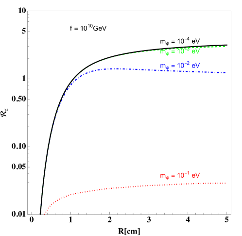
Fig. 1: Ratio $\mathcal{R}_{z}$ between the force and its classical limit as function of the size of the test object $R$, which is made of aluminum. We have fixed $f=10^{10}$ GeV, which corresponds to the skin depth $L_{\rm skin}=0.56$ cm, and plotted the ratio with $m_{\phi}=(10^{-1},10^{-2},10^{-3},10^{-4})$ eV, which corresponds to the reduced de Broglie wavelength $\bar{\lambda}_{\rm dB}=(0.2,2.0,20,200)$ cm.

Next we consider the regime

$$L_{\text{skin}}\ll R\ll\bar{\lambda}_{\text{dB}}.$$ (2.19)

We have $kR\ll 1$, so we have $s$-wave scattering, and we are still in the strong potential regime. For a spherical target of constant density, we have the textbook quantum ‘hard sphere scattering’ problem. The relevant phase shifts are given by $\delta_{0}=-kR$, $\delta_{1}=O\big{(}(kR)^{3}\big{)}$, and the force is given by

$$F_{\text{target}}=4\rho_{\phi}v_{\phi}^{2}\pi R^{2}.$$ (2.20)

Once again, this agrees with the estimate Eq. (1.1). Note that the force is 4 times larger than the classical force in this limit; this is the famous factor of 4 enhancement of the $s$-wave cross section compared to classical geometric scattering.

Next we consider the regime

$$R\ll L_{\text{skin}}\ll\bar{\lambda}_{\text{dB}}.$$ (2.21)

Because we have $R\ll L_{\text{skin}}$, the target does not strongly affect the incoming wave, and we can use the Born approximation. In this case, the scattering cross section and the force is proportional to $V_{\text{eff}}^{2}\propto 1/f^{2}$. Therefore, the scattering is highly suppressed compared to the strong potential regime, where the cross section is independent of $f$. For a sphere of radius $R$ with $kR\ll 1$, the Born scattering amplitude is given by

$$f(\theta)=-\frac{m_{\phi}}{2\pi}\int\mkern-5.0mud^{3}r\hskip 1.00006pte^{i{\mathbf{q}}\cdot{\mathbf{r}}}\hskip 1.00006ptV({\mathbf{r}})=-\frac{n_{\psi}R^{3}}{3f},$$ (2.22)

where $q=2k\sin(\theta/2)$ is the momentum transfer. The force is then given by

$$F_{\text{target}}=n_{\phi}v_{\phi}\int_{-1}^{1}d\!\hskip 0.50003pt\cos\theta\,\frac{1}{2\pi}|f(\theta)|^{2}\,m_{\phi}v_{\phi}(1-\cos\theta)=4\pi R^{2}\rho_{\phi}v_{\phi}^{2}\left(\frac{n_{\psi}R^{2}}{3f}\right)^{2}.$$ (2.23)

Note that the ratio to the maximal force is of order $(R/L_{\text{skin}})^{4}\ll 1$.

In the weak potential regime $V_{\text{eff}}\ll k^{2}/2m_{\phi}$ (or $L_{\text{skin}}\gg\bar{\lambda}_{\text{dB}}$) we can again use the Born approximation, and the force is again suppressed by $1/f^{2}$. We summarize these results for a general target of size $R$ in Table 1 and visualize different limit in Figure 1, where we have plotted the ratio $\mathcal{R}_{z}$ between the force on a solid aluminum sphere and its classical limit as function of the radius $R$.

2.3 Shielding Effects

We now give some quantitative estimates of the effect of shielding. We are interested in the strong potential regime $L_{\text{skin}}\ll\bar{\lambda}_{\text{dB}}$, since this is the only case where shielding can be significant. We will consider a shield with size $\sim R$ and thickness $\Delta R\ll R$.

To get a qualitative understanding, we consider a shield that is an infinite plane with thickness $\Delta R$ that is perpendicular to the direction of propagation of the dark matter. Computing the transmission coefficient for this case is a standard problem in non-relativistic quantum mechanics [7], and the result is (assuming $L_{\text{skin}}\ll\bar{\lambda}_{\text{dB}}$)

$$|T|^{2} =\left[1+\frac{\bar{\lambda}_{\text{dB}}^{2}}{4L_{\text{skin}}^{2}}\sinh^{2}(\Delta R/L_{\text{skin}})\right]^{-1}\simeq\begin{cases}\displaystyle\frac{16L_{\text{skin}}^{2}}{\bar{\lambda}_{\text{dB}}^{2}}e^{-2\Delta R/L_{\text{skin}}}&\Delta R\mathrel{{\mathrel{\raise 1.29167pt\hbox{$>$\kern-7.5pt\lower 4.30554pt\hbox{$\sim$}}}}}L_{\text{skin}},\\[12.0pt] \displaystyle 1-\frac{\bar{\lambda}_{\text{dB}}^{2}\Delta R^{2}}{4L_{\text{skin}}^{4}}&\Delta R\ll L_{\text{skin}}.\end{cases}$$ (2.24)

As expected, the transmission coefficient is exponentially suppressed for $\Delta R\mathrel{{\mathrel{\raise 1.29167pt\hbox{$>$\kern-7.5pt\lower 4.30554pt\hbox{$\sim$}}}}}L_{\text{skin}}$, and is is close to 1 if $\Delta R\ll L_{\text{skin}}$. This can be used to approximate the shielding effects if the size of the shield $R$ is much larger than the reduced de Broglie wavelength $\bar{\lambda}_{\text{dB}}$.

The opposite limit $\bar{\lambda}_{\text{dB}}\gg R$ is less intuitive. It is relevant only for the very lightest dark matter masses in the phenomenological regime of interest. We investigate this regime with a simple model consisting of a hollow sphere of radius $R$ and thickness $\Delta R\ll R$. To quantify the importance of the shielding, we compute the momentum density of the dark matter at the center of the sphere, $\langle T^{0z}\rangle_{r=0}$. This gives the strength of the dark matter ‘wind’ seen by a target at the center of the sphere. The solution is given in Appendix A (see Eq. (6.2)). In the large de Broglie wavelength limit, the solution is dominated by the lowest partial waves, and we obtain the ratio

$$\mathcal{R}=\mathop{\rm Re}(D_{0}^{*}D^{\vphantom{\dagger}}_{1}),$$ (2.25)

where the coefficients $D_{\ell}$ are given in Eq. (6.25c). In the limit

$$L_{\text{skin}}\ll\bar{\lambda}_{\text{dB}},\qquad R\ll\bar{\lambda}_{\text{dB}},$$ (2.26)

we find

$$\mathcal{R}=\frac{\langle T^{0z}\rangle_{r=0}}{\langle T^{0z}\rangle_{r\to\infty}}\simeq\begin{cases}\displaystyle 12\frac{L_{\text{skin}}^{2}}{R^{2}}e^{-2\Delta R/L_{\text{skin}}}&\Delta R\mathrel{{\mathrel{\raise 1.29167pt\hbox{$>$\kern-7.5pt\lower 4.30554pt\hbox{$\sim$}}}}}L_{\text{skin}},\\[10.0pt] \displaystyle 1-\frac{4}{3}\frac{R\Delta R}{L_{\text{skin}}^{2}}.&\Delta R\ll L_{\text{skin}},\end{cases}$$ (2.27)

As we expect, the result is exponentially suppressed for $\Delta R\mathrel{{\mathrel{\raise 1.29167pt\hbox{$>$\kern-7.5pt\lower 4.30554pt\hbox{$\sim$}}}}}L_{\text{skin}}$, and near 1 for $\Delta R\ll L_{\text{skin}}$. However, the coefficients differ from the infinite wall limit Eq. (2.27).

For $\Delta R\ll L_{\text{skin}}$, the deviation from 1 is of order $1/L_{\text{skin}}^{2}\sim 1/f$ rather than $1/f^{2}$ because it results from the interference of a weakly scattered wave and the unscattered wave. This is allowed because there is no unitarity constraint that relates the momentum density in the center to the scattering amplitude, as in the infinite wall case.

In Fig. 2 we show how the ratio $\mathcal{R}$ depends on the thickness of the shielding. The parameters are chosen to approximately match the satellite experiment proposed in Ref. [8], which will be discussed briefly in §4 below.

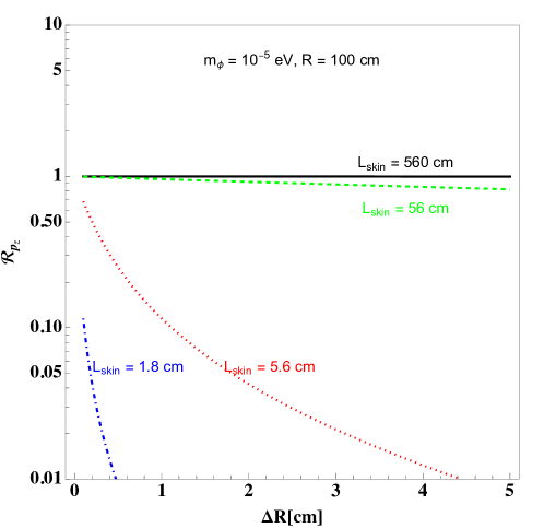
Fig. 2: Ratio $\mathcal{R}_{p_{z}}$ between the $z$-component momentum density inside a hollow sphere as functions of thickness of the shell with outer radius $R=100$ cm, which is made of Aluminum. We have fixed $m_{\phi}=10^{-4}$ eV and plotted the ratio with $f=(10^{10},10^{12},10^{14},10^{16})$ GeV.

3 Existing Constraints

In this section, we summarize constraints on the model from existing observations. Much of this section is a summary of previous work, but we also consider additional effects related to the dark Meissner effect that have not been previously considered in the literature; we find that these effects do not affect the existing constraints.

For definiteness, we consider the constraints a benchmark models with effective couplings to nucleons and electrons given by

$$\mathcal{L}_{\text{eff}}=-\left[\frac{1}{f_{n}}\bar{n}n+\frac{1}{f_{p}}\bar{p}p+\frac{1}{f_{e}}\bar{e}e\right]{\textstyle\frac{1}{2}}\phi^{2}.$$ (3.1)

For most purposes, we can assume that there is an approximately equal couplings to protons and neutrons with coefficient $f_{N}^{-1}=\frac{1}{2}(f_{n}^{-1}+f_{p}^{-1})$.

3.1 Supernova Cooling

The first constraint we consider is the cooling of stars due to $\phi$ emission. Our model contains an irrelevant interaction, and so the strongest astrophysical cooling constraint comes from supernova SN1987A, since this have the highest relevant temperature scale ($T_{\text{SN}}\sim 30$ MeV). The constraint can be approximated using the ‘Raffelt criterion’ [9], which states that the instantaneous luminosity for the new light particles with effective masses smaller than $T_{\text{SN}}$ cannot exceed the neutrino luminosity observed by the SN1987A.

For the nucleon coupling, this constraint was estimated in [10], and gives

$$f_{N}\mathrel{{\mathrel{\raise 1.29167pt\hbox{$>$\kern-7.5pt\lower 4.30554pt\hbox{$\sim$}}}}}1.1\times 10^{8}~{}\text{GeV}.$$ (3.2)

The bound for electron couplings does not appear in the literature, so we derived it using the approximations described in [10]. We constrain the production rate by

$$\Gamma(e^{+}e^{-}\rightarrow\phi\phi)\simeq\frac{7\zeta(3)T_{\text{SN}}^{7}}{320\pi f_{e}^{2}}\lesssim 10^{-14}\text{ MeV}^{5}$$ (3.3)

which leads to

$$f_{e}\mathrel{{\mathrel{\raise 1.29167pt\hbox{$>$\kern-7.5pt\lower 4.30554pt\hbox{$\sim$}}}}}1.4\times 10^{8}\,\rm GeV.$$ (3.4)

Because of the high density of the supernova core, the mass of the $\phi$ particles inside the core is much larger than the mass in vacuum. However, this does not affect the bounds in this model because the mass is still small compared to the temperature $T_{\text{SN}}$. For example, for couplings to nucleons, we have

$$\sqrt{\Delta m_{\phi}^{2}}=\sqrt{\frac{n_{N}}{f_{N}}}\sim 4~{}\text{keV}\left(\frac{f_{N}}{10^{8}~{}\text{GeV}}\right)^{-1/2},$$ (3.5)

where we assumed $n_{N}\sim 2\times 10^{38}/$cm³. The effects for the electron coupling are even weaker, since $n_{e}/n_{N}\sim 10^{-2}$.

3.2 Big Bang Nucleosynthesis

Next we consider the constraints from big bang nucleosynthesis. During nucleosynthesis $\langle\phi^{2}\rangle$ was larger than it is today, and this affects the proton-neutron mass difference and the electron mass via the couplings Eq. (3.1). The relic abundances of nuclei are very sensitive to these quantities, so this puts a bound on the parameters of the model. The nucleon and electron mass modification is given by

$$\Delta m_{\psi}=\frac{\langle\phi^{2}\rangle}{2f_{\psi}}=\frac{\rho_{\phi}}{m_{\phi}^{2}f_{\psi}},\qquad\psi=n,\,p,\,e.$$ (3.6)

where the dark matter density $\rho_{\phi}$ is fixed by the cosmological evolution. Therefore, nucleosynthesis primarily puts a bound on the parameter combination $1/m_{\phi}^{2}f_{\psi}$.

These bounds were considered in [12], and have been refined considerably since [13, 14]. For electron couplings, the constraint in the parameter region of interest to us can be summarized as

$$\frac{1}{m_{\phi}^{2}f_{e}}\mathrel{{\mathrel{\raise 1.29167pt\hbox{$<$\kern-7.5pt\lower 4.30554pt\hbox{$\sim$}}}}}9~{}\text{GeV}^{-1}\,\text{eV}^{-2}.$$ (3.7)

For the nucleon couplings, the bounds are model-dependent: they depend on the form of the couplings of $\phi$ to quarks and gluons above the QCD confinement scale. The reason is that the nucleosynthesis bounds are primarily sensitive to the neutron-proton mass difference, while the matter effects we are considering in this paper are primarily sensitive to the sum of the proton and nucleon couplings. To illustrate the range of possibilities, we consider two benchmark models, one where the $\phi$ field couples only to the down quark, and the second where it couples only to gluons:

$$\mathcal{L}_{\text{int}}=-\frac{1}{2\Lambda_{d}}\phi^{2}\bar{d}d\qquad\text{or}\qquad-\frac{1}{2\Lambda_{G}^{2}}\phi^{2}G^{\mu\nu}_{a}G_{\mu\nu a}.$$ (3.8)

Each of these models can be approximately realized by specific UV completions of the model, as discussed in Appendix B. The nucleosynthesis bounds are weaker for the second model because the gluon coupling contributes to the neutron-proton mass difference only through small isospin-breaking effects. In both models, we have $f_{p}\simeq f_{n}\simeq f_{N}$, and the respective bounds are

$$\frac{1}{m_{\phi}^{2}f_{N}}\mathrel{{\mathrel{\raise 1.29167pt\hbox{$<$\kern-7.5pt\lower 4.30554pt\hbox{$\sim$}}}}}2\times 10^{-4}~{}\text{GeV}^{-1}\,\text{eV}^{-2}\qquad\text{or}\qquad\frac{1}{m_{\phi}^{2}f_{N}}\mathrel{{\mathrel{\raise 1.29167pt\hbox{$<$\kern-7.5pt\lower 4.30554pt\hbox{$\sim$}}}}}2\times 10^{-2}~{}\text{GeV}^{-1}\,\text{eV}^{-2}.$$ (3.9)

These constraints are illustrated in Fig. 3 along with the constraints from supernova cooling.

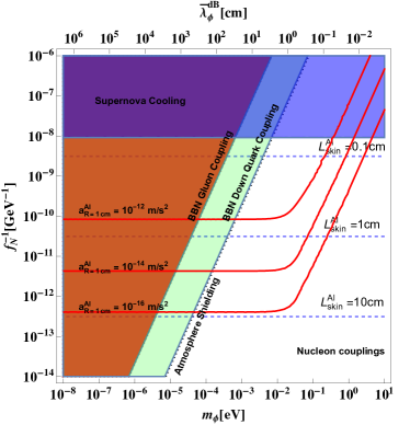
Fig. 3: Summary of constraints for couplings of $\phi$ to nucleons (left panel) and electrons (right panel). The blue regions are excluded by supernova cooling, while the red and green regions are excluded by nucleosynthesis. In the left figure, the red region corresponds to a coupling to gluons, while the green region corresponds to the coupling to the down quark. Above the black dotted line, the dark matter wind is shielded by the earth’s atmosphere. The red solid lines give the acceleration of a solid aluminum target with radius 1 cm. For comparison, the horizontal blue dashed lines give the skin depth $L_{\text{skin}}$ for aluminum.

3.3 The Dark Drag Force

Because of the dark matter Meissner effect, ordinary baryonic matter will experience a force in the dark matter rest frame that tends to make it come to rest relative to the dark matter. For obvious reasons, we call this the dark drag force. In this subsection, we consider the effect of this force on ordinary matter in a galaxy such as the Milky way.

Our galaxy consists of a dark matter halo, with ordinary matter orbiting inside the halo with speed $\sim v_{\phi}$. The dark drag force tends to make baryonic matter come to rest relative to the halo, possibly modifying galactic dynamics in an observable way.

Our galaxy contains copious amounts of gas, mostly Hydrogen. A Hydrogen molecule is far too small a target for the collective effects discussed above to be important, so the drag force can be obtained from the scattering cross section for a proton to scatter from a $\phi$ particle:

$$\Gamma=n_{\phi}v_{p}\sigma(\phi p\to\phi p)=\frac{\rho_{\phi}v_{p}}{16\pi m_{\phi}f_{p}^{2}},$$ (3.10)

where $v_{p}$ is the relative velocity of the proton relative to the dark matter.

Because $m_{p}\gg m_{\phi}$, each collision results in a transfer of kinetic energy of order $m_{\phi}v_{\text{rel}}^{2}$. The rate of energy loss of the proton is therefore

$$\frac{\dot{E}_{p}}{E_{p}}\sim\frac{\rho_{\phi}v_{p}}{16\pi f_{p}^{2}m_{p}}.$$ (3.11)

Note that this is independent of $m_{\phi}$ when expressed in terms of the dark matter density $\rho_{\phi}$. The age of a typical galaxy is of order $T_{\text{gal}}\sim 10^{10}$ years. Requiring that a typical proton orbiting the galaxy does not lose an order-1 fraction of its energy during that time gives the extremely weak constraint $f_{p}\mathrel{{\mathrel{\raise 1.29167pt\hbox{$<$\kern-7.5pt\lower 4.30554pt\hbox{$\sim$}}}}}10~{}\text{MeV}$. The constraints on electron couplings are similarly weak.

For sufficiently large objects, the collective effects become important for the drag force. To estimate this maximum size of this effect, we assume a maximal acceleration given by Eq. (1.2). For a given density $\rho$ of the object, the force is proportional to the area, while the mass is proportional to the volume, so the acceleration is proportional to $1/R$, where $R$ is the size of the object. The dark drag force is then large enough to slow the object over the lifetime of the galaxy for

$$R\mathrel{{\mathrel{\raise 1.29167pt\hbox{$<$\kern-7.5pt\lower 4.30554pt\hbox{$\sim$}}}}}\frac{\rho_{\phi}v_{\phi}T_{\text{gal}}}{\rho}\sim\text{cm}\left(\frac{\rho}{10~{}\text{g}/\text{cm}^{3}}\right)^{-1},$$ (3.12)

where we have normalized $\rho$ to the density of ordinary matter. (Note that the average density of the sun and Jupiter are both $\sim 1$ g$/$cm³, which is not so different.) Such small objects do not play an important role in the dynamics of the galaxy. It is intriguing that small chunks of ice (for example) cannot freely orbit our galaxy, but we know of no observational constraint arising from this effect.

4 Detecting the Dark Matter Wind

In this section we discuss experiments that may be able to detect the force from the dark matter wind in the parameter regime where the dark matter Meissner effect is nearly maximal. This force has multiple characteristics that can be used to separate the signal from experimental backgrounds. However, we will argue that existing experiments are not sensitive to this force due to shielding effects. We will give a general discussion of both earth-based and satellite experiments, but we will leave the question of experimental parameters and feasibility for future work.

To give an indication of the magnitude of the force, we plot the size of the acceleration of a 11 g spherical aluminum target with radius of 1 cm in Fig. 3, along with the constraints on the model discussed in §3. For comparison, the sensitivity of the Eöt-Wash torsion balance experiment for a similar target ($m\simeq 5$ g) is $\delta a\simeq 9\times 10^{-15}$ m$/$s² [2, 1]. The Microscope satellite experiment, which currently puts the strongest limits on violations of the equivalence principle, has a sensitivity of $\delta a\simeq 5\times 10^{-14}$ m$/$s², but for a larger target ($m\sim 300$ g) [15]. The upgraded version of this experiment (Galileo) is expected to increase the sensitivity by another 2 orders of magnitude [16] . We see that the accelerations that can be detected in existing or planned weak force experiments are nominally sensitive to the dark matter wind a wide range of parameter space of the model.

However, the same effect that gives rise to the force also means that the dark matter wind is shielded by ordinary matter. For example, the earth’s atmosphere will shield the dark matter wind if $\Delta m_{\phi}^{2}\sim n_{\text{atm}}/f\mathrel{{\mathrel{\raise 1.29167pt\hbox{$>$\kern-7.5pt\lower 4.30554pt\hbox{$\sim$}}}}}m_{\phi}^{2}v_{\phi}^{2}$, or

$$\frac{f^{-1}}{m_{\phi}^{2}}\mathrel{{\mathrel{\raise 1.29167pt\hbox{$>$\kern-7.5pt\lower 4.30554pt\hbox{$\sim$}}}}}10^{-4}~{}\text{GeV}^{-1}\,\text{eV}^{-2}.$$ (4.1)

This is the region above the dashed black line in Fig. 3, and terrestrial experiments will not be sensitive to the dark matter wind this regime.

The quantitative effects of shielding in an experiment cannot be determined quantitatively without modeling the experiment and its environment. Rough estimates of the shielding in existing experiments indicate that the shielding is too large for them to be sensitive to the dark matter wind. For example, torsion balance experiments take place in vibration-isolated laboratories surrounded by meters of dense matter. The masses in the Microscope experiment are surrounded by instrumentation with thickness $\sim 5$ cm, in addition to the rest of the satellite. It is clear that experiments designed to be sensitive to the force from the dark matter wind will have to be carefully designed to ensure that shielding effects are small. See Fig. 2 for a quantitative example.

We now discuss what kind of experiments might be sensitive to the force from the dark matter wind. Force experiments that search for violations of the equivalence principle are natural points of comparison, since these typically involve very precise measurements of forces on large (cm scale) targets. The acceleration due to gravity is independent of the target, while the acceleration produced by the dark matter is proportional to the area of the target and inverse proportional to its mass. In this sense, the dark matter wind induces a violation of the equivalence principle, and the dependence of the force on the target parameters is one handle to distinguish the dark matter force from gravity and background effects.

In addition, the average direction of the dark matter wind is known to be coming from the constellation Cygnus, which is visible in the northern hemisphere. Terrestrial experiments therefore have a daily modulation in the direction of the force, including the disappearance of the force when Cygnus is below the horizon. The reflection of the dark matter from the surface of the earth means that the net direction of the wind is horizontal in the approximation where the only matter near the experiment is the (nearly) flat surface of the earth. However, this is not expected to be a good approximation if there are large dense objects nearby, and modeling of the interaction of the dark matter with the experimental environment will be required to determine if there is a signal whose characteristics can be understood with sufficient accuracy to be confident that a given experiment is in fact sensitive.

For satellite-based experiments, there is a modulation once per orbit due to the orbit of the satellite. In this case, the environment consists of the earth, and the effects of the shielding and reflection of dark matter from the earth must be modeled.

In addition, both terrestrial and satellite experiments will experience an annual modulation of the signal due to the earth’s motion around the sun. The earth orbits the sun with a speed of approximately 30 km$/$s, approximately $10\%$ of the average speed of the dark matter wind. The dark matter force is proportional to the square of the wind velocity (see Eq. (1.1)), so this will give rise to a significant modulation in the magnitude of the force. The phase and magnitude of this modulation is completely calculable, and provides an additional handle on the signal.

The strong shielding of dark matter opens the possibility of controlling dark matter to increase the sensitivity of experiments. Experiments can selectively admit the dark matter through ‘windows’ with reduced shielding. If these windows can be opened and closed, this can be used to measure backgrounds in the absence of signals. In the regime where the force is maximal, the reflection of dark matter from ordinary matter is nearly perfect, and one can imagine dark matter ‘wave guides’ to bring the dark matter wind into a low-background laboratory environment in a controlled way, or trapping dark matter in a cavity. Less dramatically, the signal can be modulated by shielding that introduces a known time dependence, for example moving an inhomogeneous shield around a force detector.

One proposed experiment that we believe would be sensitive to the dark matter wind is a space mission test of the gravitational inverse-square law on a distance scale of 1–100 AU, proposed in [8]. The spacecraft is sent out of the orbital plane of the solar system, where the gravitational force is completely dominated by the sun. The experiment consists of one ‘drag free’ spacecraft that steers around a proof mass floating in its center, together with another spacecraft 10 km away that communicates ranging information to the earth. The expected sensitivity to a deviation in the radial acceleration is $\delta a\sim 4\times 10^{-17}$ m$/$s². This sensitivity benefits from the fact that the deviation from the expected geodesic orbit builds up over the many years that the distance is being measured. The drag-free spacecraft is required to have a simple spherical geometry to control various background effects. If we approximate it as a sphere of radius $\sim 1$ m with $\sim 1$ cm aluminum shielding, then the dark matter force of the proof mass will be nearly maximal for a wide range of parameters (see Fig. 2). In principle the directionality of the dark matter force can be used to distinguish it from a violation of the inverse-square law for the gravitational force, but this experiment is sensitive mainly to the distance to the earth, and hence the component of the acceleration along this direction. However, it appears that this type of experiment can be sufficiently light shielding together with sensitivity to acceleration to observe the dark matter wind.

An upgraded version of this experiment with two drag-free spacecraft and one relay spacecraft that ranges the distance to the drag-free spacecraft could presumably measure the distance between the two drag-free spacecraft with at least as good an accuracy as the distance to the earth, and therefore would independently measure the relative acceleration of the drag-free spacecraft, and thereby distinguish the dark matter force from a modified gravitational acceleration. We hope that the possibility of measuring the force from dark matter will give an additional motivation for building this kind of experiment.

5 Conclusions

In this paper, we have explored a model of dark matter where the interaction between dark matter and ordinary matter can be maximally strong, in the sense that dark matter scatters elastically from sufficiently dense and large matter targets. The dark matter in this model consists of a scalar $\phi$ with mass $m_{\phi}\mathrel{{\mathrel{\raise 1.29167pt\hbox{$<$\kern-7.5pt\lower 4.30554pt\hbox{$\sim$}}}}}\text{eV}$ and an effective coupling to nucleons and/or electrons given by Eq. (1.3). This coupling increases the mass of the $\phi$ particle inside ordinary matter, which suppresses the propagation of dark matter inside the target and can lead to elastic scattering. This is a collective effect due to the coherent scattering of the dark matter from many nucleons/electrons. It is similar to the Meissner effect that gives photons a mass inside a superconductor, so we call it the ‘dark Meissner effect.’

Because of the rotation of the Milky Way inside the dark matter halo, the dark matter around the earth is moving with an average velocity $v_{\phi}\sim 300$ km$/$s from the direction of Cygnus. The maximal force from this dark matter ‘wind’ that arises for elastic scattering is very small (see Eq. (1.2)), but is large enough to be detected in sensitive force measurements. However, the strong interaction between dark matter and ordinary matter also means that the dark matter is shielded from existing experiments.

We have shown how this force can be computed quantitatively, using both the classical and quantum pictures for the dark matter. We present a number of explicit calculations to illustrate how the force depends on the dark matter de Broglie wavelength, target size and density, amount of shielding, etc. These calculations confirm that the dark matter force can indeed be maximal in a wide range of parameters. Based on these estimates, we believe that existing fifth force experiments (both terrestrial and satellite based) are not sensitive to the dark matter force because of shielding effects. We also show that this model is consistent with astrophysical and cosmological constraints in a region where the force is large enough to be observed experimentally (see Fig. 3).

This leads us to consider a novel experimental signal of dark matter: multiple elastic scatterings of dark matter from ordinary matter that are accumulated during a long period of time, leading to a collective force that can be detected using sensitive force experiments. This is a unique signal with many characteristics that can be used to distinguish it from backgrounds: the force has a known direction, annual modulation due to the earth’s orbit, and time dependence due to the earth’s shadow. Perhaps most uniquely, the force is proportional to the area of the target, and dark matter can be shielded and/or controlled by ordinary matter. Detecting such a signal would not only give direct evidence of dark matter, but also information about its local velocity distribution.

To detect this signal, one needs a sufficiently sensitive force probe that is not too shielded from the dark matter wind. The size of the force to be measured is larger than forces already probed in these experiments, and we see no insurmountable obstacle to building such an experiment. We do not propose a specific experimental design to search for this signal in this paper, leaving this for future work. We hope that our results will stimulate work in this direction.

Note: As we were completing this work, we became aware of Ref. [17], which demonstrates that the force mediated by the $\phi$ field has a range of order the de Broglie wavelength (rather than the Compton wavelength) due to the presence of a background $\phi$ field. That work does not give results for the case where the collective effects discussed in this paper are important. Ref. [17] also gives a stronger bound on the $\phi^{4}$ coupling from the bullet cluster, modifying the tuning estimates in our Appendix B.

Appendix A: Calculations and Results

In this appendix, we collect additional details about the calculation of the force due to the dark matter wind. We also present results of calculations for particular cases.

We are interested in steady-state solutions of the form Eq. (2.10) that describe scattering of an incident wave in the $+z$ direction. This means that $\psi({\mathbf{r}})$ has the form

$$\psi({\mathbf{r}})=\phi_{0}\Big{[}e^{ikz}+\psi_{\text{scatt}}({\mathbf{r}})\Big{]},$$ (6.1)

where $k=m_{\phi}v_{\phi}$. The classical equations of motion for $\phi$ imply that $\psi({\mathbf{r}})$ satisfies the non-relativistic Schrödinger equation, Eqs. (2.12) and (2.13). This leads to the equivalence between the force computed in the classical and quantum pictures, as we will see.

Finding the solution to this problem is a standard problem in non-relativistic quantum mechanics. At large distances where the matter density vanishes, the scattered wave can be written as

$$\psi_{\text{scatt}}({\mathbf{r}})=\sum_{\ell\,=\,0}^{\infty}i^{\ell}(2\ell+1)P_{\ell}(\cos\theta)A_{\ell}\Big{[}j_{\ell}(kr)+iy_{\ell}(kr)\Big{]},$$ (6.2)

where we have defined

$$A_{\ell}=\frac{S_{\ell}-1}{2}.$$ (6.3)

Here $S_{\ell}$ is the quantum-mechanical $S$-matrix element for the partial wave $\ell$ (see Eq. (2.16)). Here $j_{\ell}$ ($y_{\ell}$) are the spherical Bessel functions of the first (second) kind, and $P_{\ell}$ are the Legendre polynomials. Eqs. (6.1) and (6.2) can be understood from the partial wave expansion of the full solution:

$$\psi({\mathbf{r}})=\phi_{0}\sum_{\ell}i^{\ell}(2\ell+1)C_{\ell}(r)P_{\ell}(\cos\theta),$$ (6.4)

where the partial waves for $r\to\infty$ are given by

$$C_{\ell}(r)=j_{\ell}(kr)+A_{\ell}\big{[}j_{\ell}(kr)+iy_{\ell}(kr)\big{]}\to\frac{e^{-i(kr-\ell\pi/2)}+S_{\ell}e^{i(kr-\ell\pi/2)}}{2ikr}.$$ (6.5)

This corresponds to a phase shift $S_{\ell}$ for the outgoing wave.

The solution above describes both the classical $\phi$ field, and also the wavefunction for a single $\phi$ particle in the quantum picture. However, the calculation of the force is different in the two pictures. In the classical formulation, we compute the force on the target by computing the momentum transferred to the target by the field. In the presence of the target, the spatial components of the energy-momentum tensor of the $\phi$ field are not conserved:

$$\partial_{\mu}T^{\mu i}_{\phi}=-\frac{\partial_{i}n({\mathbf{r}})}{2f}\phi^{2},$$ (6.6)

where $T^{\mu\nu}_{\phi}$ is the energy momentum tensor for the $\phi$ field

$$T^{\mu\nu}_{\phi}=\partial^{\mu}\phi\partial^{\nu}\phi-\eta^{\mu\nu}\mathcal{L}_{\phi},\qquad\mathcal{L}_{\phi}=\frac{1}{2}(\partial\phi)^{2}-\frac{1}{2}\big{(}m_{\phi}^{2}+n({\mathbf{r}})/f\big{)}\phi^{2}.$$ (6.7)

Therefore, the presence of a target transfers momentum to the field. The force on the target can therefore be obtained from the momentum transfer to the field:

$$F^{i}_{\text{target}}=-\frac{d}{dt}P_{\phi}^{i}=-\int\mkern-5.0mudA\,T_{\phi}^{ij}\hat{n}^{j}.$$ (6.8)

The integration surface is taken in a region where $n({\mathbf{r}})=0$, so $T^{\mu\nu}_{\phi}$ is conserved and the integral is independent of the choice of surface. We can therefore evaluate the integral over a sphere with radius $r\to\infty$. Because $dA\propto r^{2}$, the only terms that contribute are those where $T^{\mu\nu}_{\phi}\sim 1/r^{2}$.

Because we are interested in the force on time scales $t\gg 1/\omega$, we will average over the oscillations in time. The averaged components of the energy-momentum tensor are given by

$$\langle T^{00}_{\phi}\rangle ={\textstyle\frac{1}{4}}\Big{[}(\omega^{2}+m_{\phi}^{2})|\psi|^{2}+|{\mathbf{\nabla}}\psi|^{2}\Big{]},$$ (6.9a)

$$\langle T^{ij}_{\phi}\rangle =\langle T_{\phi\hskip 0.70004ptij}\rangle={\textstyle\frac{1}{4}}\Big{[}\partial_{i}\psi^{*}\partial_{j}\psi+\partial_{j}\psi^{*}\partial_{i}\psi-{\textstyle\frac{1}{2}}\delta_{ij}{\mathbf{\nabla}}^{2}|\psi|^{2}\Big{]},$$ (6.9b)

where $i,j$ are Cartesian spatial indices. The force on the target is in the $z$ direction, so we can write

$$\langle F_{\text{target}}^{z}\rangle =-\int\mkern-5.0mudA\hskip 1.00006pt\langle T^{zi}_{\phi}\rangle\hat{r}^{i}$$

$$=-2\pi r^{2}\int_{-1}^{1}\!d\!\hskip 0.50003pt\cos\theta\,{\textstyle\frac{1}{4}}\Big{[}\big{(}\partial_{z}\psi^{*}\partial_{r}\psi+\mathrm{h.c.}\big{)}-{\textstyle\frac{1}{2}}{\mathbf{\nabla}}^{2}|\psi|^{2}\cos\theta\Big{]}.$$ (6.10)

Because the integral is over a surface with $r\to\infty$, only the terms $\sim 1/r^{2}$ in the integrand contribute.

Keeping only the leading terms in the expansion in $1/r$ in the partial wave expansion is equivalent to using the approximations

$$\partial_{z}\psi\simeq\cos\theta\partial_{r}\psi,\qquad{\mathbf{\nabla}}^{2}|\psi|^{2}\simeq\partial_{r}^{2}|\psi|^{2},$$ (6.11)

which gives

$$F_{\text{target}}^{z} =-\frac{\pi r^{2}}{2}\int_{-1}^{1}\!d\!\hskip 0.50003pt\cos\theta\,\Big{[}|\partial_{r}\psi|^{2}-{\textstyle\frac{1}{2}}\big{(}\psi^{*}\partial_{r}^{2}\psi+\mathrm{h.c.}\big{)}\Big{]}\cos\theta+O(1/r).$$ (6.12)

We use the identities

$$j^{\prime}_{\ell}(\rho)=-j_{\ell+1}(\rho)+\frac{\ell}{\rho}j_{\ell}(\rho),\qquad y^{\prime}_{\ell}(\rho)=-y_{\ell+1}(\rho)+\frac{\ell}{\rho}y_{\ell}(\rho),$$ (6.13)

and the asymptotic forms of the spherical Bessel functions to obtain

$$(\partial_{r})^{n}\psi=-\frac{i\phi_{0}}{2kr}(ik)^{n}\sum_{\ell}(2\ell+1)P_{\ell}(\cos\theta)\Big{[}S_{\ell}e^{ikr}-(-1)^{\ell+n}e^{-ikr}\Big{]}+O(1/r^{2}).$$ (6.14)

The angular average is performed using the identity

$$\int_{-1}^{1}d\!\hskip 0.50003pt\cos\theta\,P_{\ell}(\cos\theta)P_{\ell^{\prime}}(\cos\theta)\cos\theta=\begin{cases}\displaystyle\frac{2\max(\ell,\ell^{\prime})}{(\ell+\ell^{\prime})(\ell+\ell^{\prime}+2)}&\ell-\ell^{\prime}=\pm 1,\\[12.0pt] 0&\text{otherwise},\end{cases}$$ (6.15)

and we obtain

$$F^{z}_{\text{target}}=-2\pi|\phi_{0}|^{2}\sum_{\ell}(\ell+1)\Big{[}S_{\ell}^{*}S^{\vphantom{\dagger}}_{\ell+1}+S_{\ell+1}^{*}S^{\vphantom{\dagger}}_{\ell}-2\Big{]}.$$ (6.16)

With the normalization Eq. (2.15), this gives the result Eq. (2.14) for the force.

We now compare this to the momentum transfer computed in the quantum mechanics picture. In this picture, the momentum is transferred to the target by the scattering of individual $\phi$ particles. The scattering cross section is determined by the $r\to\infty$ behavior of the scattered wave

$$\psi_{\text{scatt}}({\mathbf{r}})\to\frac{e^{ikr}}{r}f(\theta),\qquad f(\theta)=\frac{1}{2ik}\sum_{\ell}(2\ell+1)P_{\ell}(\cos\theta)(S_{\ell}-1).$$ (6.17)

The differential scattering cross section is given by

$$\frac{d\sigma}{d\Omega}=\frac{1}{2\pi}\frac{d\sigma}{d\cos\theta}=|f(\theta)|^{2},$$ (6.18)

so the momentum transferred to the target is given by

$$F^{z}_{\text{target}} =n_{\phi}v_{\phi}\int_{-1}^{1}d\!\hskip 0.50003pt\cos\theta\,\frac{d\sigma}{d\cos\theta}\hskip 1.00006ptm_{\phi}v_{\phi}(1-\cos\theta)$$

$$=-\frac{\pi\rho_{\phi}}{m_{\phi}^{2}}\sum_{\ell}(\ell+1)\Big{[}S_{\ell}^{*}S^{\vphantom{\dagger}}_{\ell+1}+S_{\ell+1}^{*}S^{\vphantom{\dagger}}_{\ell}-2\Big{]},$$ (6.19)

where we used $k=m_{\phi}v_{\phi}$. This agrees with the classical result Eq. (2.14).

6.1 Solid sphere

We first consider scattering from a sphere of radius $R$ and number density $n_{0}$. This is a standard problem in quantum mechanics. The wavefunction $\psi({\mathbf{r}})$ outside the sphere is given by the expansion Eq. (6.2), while the wavefunction inside is given by

$$\psi_{r<R}(\mathbf{r})=\phi_{0}\sum_{\ell}(2\ell+1)i^{\ell}B_{\ell}j_{\ell}(\tilde{k}r)P_{\ell}(\cos\theta),$$ (6.20)

where

$$\tilde{k}=\sqrt{k^{2}-n_{0}/f\,}.$$ (6.21)

Note that the wavefunction for $r<R$ does not have a $y_{\ell}$ term because this is singular at the origin. The coefficients $A_{\ell}$ (which are equivalent to $S_{\ell}$, see Eq. (6.3)) and $B_{\ell}$ that define the solution are obtained by requiring that the wavefunction and its first derivative are continuous at $r=R$. The result is

$$A_{\ell} =\frac{-kj_{\ell}(\tilde{k}R)j_{\ell}^{\prime}(kR)+\tilde{k}j_{\ell}^{\prime}(\tilde{k}R)j_{\ell}(kR)}{kj_{\ell}(\tilde{k}R)h_{\ell}^{(1)\prime}(kR)-\tilde{k}j_{\ell}^{\prime}(\tilde{k}R)h^{(1)}_{\ell}(kR)},$$ (6.22a)

$$B_{\ell} =\frac{kh^{\prime}_{\ell}(kR)j_{\ell}(kR)-kj^{\prime}_{\ell}(kR)h_{\ell}(kR)}{kh^{\prime}_{\ell}(kR)j_{\ell}(\tilde{k}R)-\tilde{k}j^{\prime}_{\ell}(\tilde{k}R)h_{\ell}(kR)}.$$ (6.22b)

6.2 Hollow sphere

To model shielding effects, we now consider a spherical shell with inner radius $R_{1}$, outer radius $R_{2}$, and density $n_{0}$:

$$n(r)=n_{0}\big{[}\theta(R_{2}-r)-\theta(R_{1}-r)\big{]}.$$ (6.23)

Here we are interested in computing the momentum density $\langle T^{0z}\rangle$ at the center of the sphere (see Fig. 2). We have

$$\psi_{r>R_{2}}(\mathbf{r}) =\phi_{0}\sum_{\ell}(2\ell+1)i^{\ell}\left[j_{\ell}(kr)+A_{\ell}h_{\ell}^{(1)}(kr)\right]P_{\ell}(\cos\theta),$$ (6.24a)

$$\psi_{R_{1}<r<R_{2}}(\mathbf{r}) =\phi_{0}\sum_{\ell}(2\ell+1)i^{\ell}\left[B_{\ell}j_{\ell}(\tilde{k}r)+C_{\ell}y_{\ell}(\tilde{k}r)\right]P_{\ell}(\cos\theta),$$ (6.24b)

$$\psi_{r<R_{1}}(\mathbf{r}) =\phi_{0}\sum_{\ell}(2\ell+1)i^{\ell}D_{\ell}j_{\ell}(kr)P_{\ell}(\cos\theta).$$ (6.24c)

The wavefunction and its first derivative must be continuous at both the inner and outer surfaces, and we obtain

$$A_{\ell} =\frac{\tilde{k}j_{\ell}(kR_{2})\left(j_{\ell}^{\prime}(\tilde{k}R_{2})+N_{\ell}y_{\ell}^{\prime}(\tilde{k}R_{2})\right)-kj_{\ell}^{\prime}(kR_{2})\left(j_{\ell}(\tilde{k}R_{2})+N_{\ell}y_{\ell}(\tilde{k}R_{2})\right)}{kh_{\ell}^{(1)\prime}(kR_{2})\left(j_{\ell}(\tilde{k}R_{2})+N_{\ell}y_{\ell}(\tilde{k}R_{2})\right)-h_{\ell}^{(1)}(kR_{2})\left(\tilde{k}j_{\ell}^{\prime}(\tilde{k}R_{2})+N_{\ell}\tilde{k}y_{\ell}^{\prime}(\tilde{k}R_{2})\right)},$$ (6.25a)

$$B_{\ell} =\frac{kj_{\ell}(kR_{2})h_{\ell}^{(1)\prime}(kR_{2})-kj_{\ell}^{\prime}(kR_{2})h_{\ell}^{(1)}(kR_{2})}{kh_{\ell}^{(1)\prime}(kR_{2})\left(j_{\ell}(\tilde{k}R_{2})+N_{\ell}y_{\ell}(\tilde{k}R_{2})\right)-h_{\ell}^{(1)}(kR_{2})\left(\tilde{k}j_{\ell}^{\prime}(\tilde{k}R_{2})+N_{\ell}\tilde{k}y_{\ell}^{\prime}(\tilde{k}R_{2})\right)},$$ (6.25b)

$$C_{\ell} =B_{\ell}N_{\ell},\quad D_{\ell}=\frac{B_{\ell}}{j_{\ell}(kR_{1})}\left[j_{\ell}(\tilde{k}R_{1})+N_{\ell}y_{\ell}(\tilde{k}R_{1})\right],$$ (6.25c)

where $N_{\ell}$ is given by

$$N_{\ell}=\frac{kj_{\ell}^{\prime}(kR_{1})j_{\ell}(\tilde{k}R_{1})-\tilde{k}j_{\ell}^{\prime}(\tilde{k}R_{1})j_{\ell}(kR_{1})}{\tilde{k}y_{\ell}^{\prime}(\tilde{k}R_{1})j_{\ell}(kR_{1})-kj_{\ell}^{\prime}(kR_{1})y_{\ell}(\tilde{k}R_{1})}.$$ (6.26)

The momentum density inside the hollow sphere ($r<R_{1}$) is given by directly using Eq. (6.9b):

$$\langle T^{0z}(r,\theta)\rangle =\rho_{\phi}v_{\phi}\sum_{\ell\neq\ell^{\prime}}(2\ell+1)(2\ell^{\prime}+1)\mathop{\rm Re}\!\big{[}i^{\ell^{\prime}+\ell-1}D_{\ell}^{*}D^{\vphantom{\dagger}}_{\ell^{\prime}}\big{]}j_{\ell}(kr)P_{\ell}(\cos\theta)$$

$$\qquad\qquad\qquad{}\times\left[j^{\prime}_{\ell^{\prime}}(kr)\cos\theta P_{\ell^{\prime}}(\cos\theta)+\frac{j_{\ell^{\prime}}(kr)}{kr}\sin^{2}\theta P^{\prime}_{\ell^{\prime}}(\cos\theta)\right].$$ (6.27)

Appendix B: UV Completions

In this appendix, we consider two possible UV completions of the effective interactions Eq. (1.3) and show how they connect with the different cases for the nucleosynthesis bound discussed in §3. We also briefly discuss the tuning in these models.

As one would expect for a model of a light scalar with non-derivative couplings, the mass $m_{\phi}$ is very fine-tuned. The dark matter relic abundance depends sensitively on $m_{\phi}$ (for example through the misalignment mechanism [18, 19, 20]), so this tuning may have an anthropic origin [21]. On the other hand, a coupling of the form

$$\Delta\mathcal{L}=-\frac{\lambda_{\phi}}{4!}\phi^{4}$$ (7.1)

is allowed by all symmetries and is also UV sensitive. This coupling is tightly constrained by constraints from structure formation [22]

$$\lambda_{\phi}\mathrel{{\mathrel{\raise 1.29167pt\hbox{$<$\kern-7.5pt\lower 4.30554pt\hbox{$\sim$}}}}}3\times 10^{-7}\left(\frac{m_{\phi}}{\mathrm{~{}eV}}\right)^{4}.$$ (7.2)

A value of $\lambda_{\phi}$ that violates this bound modifies the spectrum of density fluctuations, but structure formation still takes place, so there is no obvious anthropic constraint on $\lambda_{\phi}$.

The simplest UV completion of the model comes from adding the scalar $\phi$ to the Standard Model with the most general renormalizable couplings compatible with the $\phi\mapsto-\phi$ symmetry:

$$\Delta\mathcal{L}_{\text{SM}}=-{\textstyle\frac{1}{2}}m_{\phi}^{2}\phi^{2}-\frac{\lambda_{\phi}}{4!}\phi^{4}-{\textstyle\frac{1}{2}}\epsilon\phi^{2}H^{\dagger}H.$$ (7.3)

This gives a $\phi$ dependent shift in the Higgs VEV:

$$\frac{\delta v}{v}=\frac{\epsilon\phi^{2}}{2m_{h}^{2}},$$ (7.4)

where $m_{h}=125$ GeV is the physical Higgs mass. Below the electroweak symmetry breaking scale, this induces various couplings of $\phi^{2}$ to standard model fields. For example, the coupling to SM fermions $\psi$ is given by

$$\Delta\mathcal{L}_{\text{eff}}=-\sum_{\psi}\frac{1}{2f_{\psi}}\phi^{2}\bar{\psi}\psi\qquad\frac{1}{f_{\psi}}=\frac{\epsilon\hskip 0.50003ptm_{\psi}}{m_{h}^{2}}.$$ (7.5)

For light fermions such as the electron and the up and down quarks, this is suppressed by the fermion mass. The low-energy couplings that are not suppressed in this way are couplings to the SM gauge field strength operators, for example $\phi^{2}G^{\mu\nu}_{a}G^{\vphantom{\dagger}}_{\mu\nu a}$, where $G_{\mu\nu a}$ is the gluon field strength. Integrating out the heavy quarks gives a common contribution to the neutron and proton masses

$$\frac{1}{f_{p}}\simeq\frac{1}{f_{n}}\simeq\frac{2}{9}\frac{\epsilon\hskip 0.50003ptm_{p}}{m_{h}^{2}}.$$ (7.6)

At low energies, this model dominantly couples to the nucleons, and this coupling is approximately isospin preserving. This corresponds to the weaker nucleosynthesis constraint in the left panel of Fig. 3.

In this model, the $\phi^{4}$ coupling has a UV divergent 1-loop contribution of order

$$\Delta\lambda_{\phi}\sim\frac{\epsilon^{2}}{16\pi^{2}}\ln\frac{\Lambda_{\text{UV}}}{m_{h}},$$ (7.7)

where $\Lambda_{\text{UV}}$ is the UV cutoff, which we identify with the scale of new physics. Comparing this to the bound Eq. (7.2) from structure formation we have

$$\frac{\Delta\lambda_{\phi}}{\lambda_{\phi\hskip 0.35002pt\text{bound}}}\sim 10^{-6}\left(\frac{m_{\phi}}{\text{eV}}\right)^{-4}\left(\frac{f}{10^{10}\mathrm{~{}GeV}}\right)^{-2},$$ (7.8)

where we have assumed that $\log(\Lambda_{\text{UV}}/m_{h})\sim 1$. As long as this is ratio is smaller than 1, the model is not fine-tuned.

Next, we consider another UV completion which can dominantly couple to electrons at low energies. This comes from adding the following interaction to the SM:

$$\mathcal{L}_{\text{SM}}=-\frac{1}{2M_{e}^{2}}\phi^{2}(LHe^{c}+\mathrm{h.c.}).$$ (7.9)

This requires UV completion at a scale of order $M_{e}$, so we require $M_{e}\mathrel{{\mathrel{\raise 1.29167pt\hbox{$>$\kern-7.5pt\lower 4.30554pt\hbox{$\sim$}}}}}\text{TeV}$. Below the electroweak symmetry breaking scale, this generates a coupling of $\phi^{2}$ to the electron given by

$$\frac{1}{f_{e}}=\frac{m_{e}}{M_{e}^{2}}.$$ (7.10)

In this UV completion, the dark matter couples dominantly to the electron at low energies.

We now discuss the fine-tuning of the quartic coupling in this model. The dominant UV divergent contribution is given by a 2-loop diagram, and is of order

$$\Delta\lambda_{\phi}\sim\left(\frac{1}{16\pi^{2}}\right)^{2}\frac{\Lambda_{\text{UV}}^{4}}{M^{4}}$$ (7.11)

which gives

$$\frac{\Delta\lambda_{\phi}}{\lambda_{\phi\hskip 0.35002pt\text{bound}}}\sim\left(\frac{m_{\phi}}{\text{eV}}\right)^{-4}\left(\frac{\Lambda_{\text{UV}}}{\text{TeV}}\right)^{4}\left(\frac{f}{10^{10}\mathrm{~{}GeV}}\right)^{-2}.$$ (7.12)

A variation of this model is to couple dominantly to a light quark, for example the down quark:

$$\mathcal{L}_{\text{SM}}=-\frac{1}{2M_{d}^{2}}\phi^{2}(QHd^{c}+\mathrm{h.c.}).$$ (7.13)

Below the electroweak symmetry breaking scale, the dominant coupling is to the down quark, with

$$\frac{1}{f_{d}}=\frac{m_{d}}{M_{d}^{2}}.$$ (7.14)

This violates isospin maximally, corresponding to the stronger nucleosynthesis bound in the left panel of Fig. 3.

References

- [1] T. A. Wagner, S. Schlamminger, J. H. Gundlach, and E. G. Adelberger, “Torsion-balance tests of the weak equivalence principle,” Class. Quant. Grav. 29 (2012) 184002, arXiv:1207.2442 [gr-qc].
- [2] S. Schlamminger, K. Y. Choi, T. A. Wagner, J. H. Gundlach, and E. G. Adelberger, “Test of the equivalence principle using a rotating torsion balance,” Phys. Rev. Lett. 100 (2008) 041101, arXiv:0712.0607 [gr-qc].
- [3] J. G. Lee, E. G. Adelberger, T. S. Cook, S. M. Fleischer, and B. R. Heckel, “New Test of the Gravitational Law at Separations down to 52 m,” Phys. Rev. Lett. 124 no. 10, (2020) 101101, arXiv:2002.11761 [hep-ex].
- [4] P. W. Graham, D. E. Kaplan, J. Mardon, S. Rajendran, and W. A. Terrano, “Dark Matter Direct Detection with Accelerometers,” Phys. Rev. D 93 no. 7, (2016) 075029, arXiv:1512.06165 [hep-ph].
- [5] D. Carney, A. Hook, Z. Liu, J. M. Taylor, and Y. Zhao, “Ultralight dark matter detection with mechanical quantum sensors,” New J. Phys. 23 no. 2, (2021) 023041, arXiv:1908.04797 [hep-ph].
- [6] H. Fukuda, S. Matsumoto, and T. T. Yanagida, “Direct Detection of Ultralight Dark Matter via Astronomical Ephemeris,” Phys. Lett. B 789 (2019) 220–227, arXiv:1801.02807 [hep-ph].
- [7] L. D. Landau and E. M. Lifshits, Quantum Mechanics: Non-Relativistic Theory, vol. v.3 of Course of Theoretical Physics. Butterworth-Heinemann, Oxford, 1991.
- [8] B. Buscaino, D. DeBra, P. W. Graham, G. Gratta, and T. D. Wiser, “Testing long-distance modifications of gravity to 100 astronomical units,” Phys. Rev. D 92 no. 10, (2015) 104048, arXiv:1508.06273 [gr-qc].
- [9] G. G. Raffelt, “Astrophysical methods to constrain axions and other novel particle phenomena,” Phys. Rept. 198 (1990) 1–113.
- [10] K. A. Olive and M. Pospelov, “Environmental dependence of masses and coupling constants,” Phys. Rev. D 77 (2008) 043524, arXiv:0709.3825 [hep-ph].
- [11] W. DeRocco, P. W. Graham, and S. Rajendran, “Exploring the robustness of stellar cooling constraints on light particles,” Phys. Rev. D 102 no. 7, (2020) 075015, arXiv:2006.15112 [hep-ph].
- [12] Y. V. Stadnik and V. V. Flambaum, “Can dark matter induce cosmological evolution of the fundamental constants of Nature?,” Phys. Rev. Lett. 115 no. 20, (2015) 201301, arXiv:1503.08540 [astro-ph.CO].
- [13] S. Sibiryakov, P. Sørensen, and T.-T. Yu, “BBN constraints on universally-coupled ultralight scalar dark matter,” JHEP 12 (2020) 075, arXiv:2006.04820 [hep-ph].
- [14] T. Bouley, P. Sørensen, and T.-T. Yu, “Constraints on ultralight scalar dark matter with quadratic couplings,” JHEP 03 (2023) 104, arXiv:2211.09826 [hep-ph].
- [15] MICROSCOPE Collaboration, P. Touboul et al., “MICROSCOPE Mission: Final Results of the Test of the Equivalence Principle,” Phys. Rev. Lett. 129 no. 12, (2022) 121102, arXiv:2209.15487 [gr-qc].
- [16] A. M. Nobili et al., “’Galileo Galilei’ (GG): Space test of the weak equivalence principle to 10(-17) and laboratory demonstrations,” Class. Quant. Grav. 29 (2012) 184011.
- [17] K. Van Tilburg, “Wake Forces,” arXiv:2312.xxxx.
- [18] J. Preskill, M. B. Wise, and F. Wilczek, “Cosmology of the Invisible Axion,” Phys. Lett. B 120 (1983) 127–132.
- [19] L. F. Abbott and P. Sikivie, “A Cosmological Bound on the Invisible Axion,” Phys. Lett. B 120 (1983) 133–136.
- [20] M. Dine and W. Fischler, “The Not So Harmless Axion,” Phys. Lett. B 120 (1983) 137–141.
- [21] B. Freivogel, “Anthropic Explanation of the Dark Matter Abundance,” JCAP 03 (2010) 021, arXiv:0810.0703 [hep-th].
- [22] A. Arvanitaki, J. Huang, and K. Van Tilburg, “Searching for dilaton dark matter with atomic clocks,” Phys. Rev. D 91 no. 1, (2015) 015015, arXiv:1405.2925 [hep-ph].