An analytic description of substructure-induced gravitational perturbations of hot stellar systems

Abstract

Perturbations to stellar systems can reflect the gravitational influence of dark matter substructures. Whereas perturbations to cold stellar systems are the most commonly studied, the sources of perturbations to dynamically hot systems are less ambiguous because such systems cannot support persistent inhomogeneity on small scales. We point out a simple algebraic relationship between the two-point statistics of a hot stellar system and those of the perturbing matter. The density and velocity power spectra of the stars are proportional to the density power spectrum of the perturbers, scaled by $k^{-4}$. This relationship allows easy evaluation of the suitability of a stellar system for detecting dark substructure. As examples, we show that the Galactic stellar halo is expected to be sensitive to cold dark matter substructure at wave numbers $k\lesssim 0.4$ kpc^-1, and the Galactic disk might be sensitive to substructure at wave numbers $k\sim 4$ kpc^-1. These systems could provide direct measurements of the nonlinear matter power spectrum at these wave numbers.

1 Introduction

Dark matter has no known nongravitational interaction with Standard Model particles. Consequently, an important experimental strategy is to infer the properties of the dark matter from its gravitational influence alone. If the dark matter is cold, it should cluster on scales much smaller than galaxies, forming collapsed and tightly bound haloes that contain no visible matter at all. Such dark haloes could be detected gravitationally, but unambiguous detection remains elusive.

A longstanding approach is to search for the gravitational influence of dark structures on visible systems of stars. Heating of dwarf galaxies by dark haloes has been considered (Starkenburg & Helmi, 2015), as has heating of star clusters (Peñarrubia, 2019; Webb et al., 2019), of tidal streams of stars (Ibata et al., 2002; Johnston et al., 2002; Carlberg, 2009; Carlberg & Agler, 2023), and of binary star systems (Penarrubia et al., 2010; González-Morales et al., 2013; Ramirez & Buckley, 2023). We focus on a refinement of this approach, which is to consider inhomogeneity induced by the gravitational influence of the dark structures. Tidal streams are the most common target for this strategy (Siegal-Gaskins & Valluri, 2008; Yoon et al., 2011; Carlberg, 2012; Ngan & Carlberg, 2014; Erkal & Belokurov, 2015; Carlberg, 2016; Erkal et al., 2016; Sanders et al., 2016; Bovy et al., 2017; Banik et al., 2018; Banik & Bovy, 2019; Bonaca et al., 2019; De Boer et al., 2020; Banik et al., 2021a, b; Koppelman & Helmi, 2021; Li et al., 2021; Malhan et al., 2021; Delos & Schmidt, 2022; Doke & Hattori, 2022; Ferguson et al., 2022; Montanari & García-Bellido, 2022; Tavangar et al., 2022), although galactic disks (e.g. Chequers et al., 2018; Tremaine et al., 2023) and spheroids (Bazarov et al., 2022; Davies et al., 2023) have been considered as well.

We use analytic methods to derive how the statistics of a gravitationally perturbed stellar system are related to those of the perturbing matter distribution. We focus on dynamically hot systems, employing approximations that are appropriate when perturbations cannot outlast the orbital time scale. Despite their popularity as probes of dark substructure, cold stellar streams can develop inhomogeneity for a range of other reasons as well (Capuzzo Dolcetta et al., 2005; Küpper et al., 2008, 2010, 2012; Amorisco et al., 2016; Pearson et al., 2017; Ibata et al., 2020; Qian et al., 2022; Weatherford et al., 2023). For hot systems, sources of inhomogeneity are easier to disambiguate due to the short lifetimes of perturbations.

We find a simple analytic relationship between the gravitationally induced perturbations of a stellar system and the properties of the perturbing structures. The power spectra of the stellar density and velocity fields become algebraically related to the power spectrum of the perturber density field. By comparing these induced power spectra to the intrinsic Poisson noise associated with the number of stars, one can easily test the sensitivity of a stellar system as a probe of dark substructure.

2 Statistics of the gravitational field

We begin by quantifying the spatial and temporal structure of the gravitational field induced by a perturbing matter system. Let $\rho(\bm{x})$ be the matter density field, where $\bm{x}$ is position. It induces gravitational acceleration

$$\bm{a}(\bm{x}) =G\int\mathrm{d}^{3}\bm{x}^{\prime}\rho(\bm{x}^{\prime})\frac{\bm{x}^{\prime}-\bm{x}}{|\bm{x}^{\prime}-\bm{x}|^{3}},$$ (1)

as a function of position $\bm{x}$, or

$$\bm{a}(\bm{k}) =4\pi\mathrm{i}G\rho(\bm{k})\bm{k}/k^{2}$$ (2)

in Fourier space, where $\rho(\bm{k})\equiv\int\mathrm{d}^{3}\bm{x}\,\mathrm{e}^{-\mathrm{i}\bm{k}\cdot\bm{x}}\rho(\bm{x})$ is the Fourier transform of $\rho(\bm{x})$. Now suppose the field is moving at velocity $\bm{u}$. As a function of time $t$, the acceleration induced by this field is

$$\bm{a}(\bm{k},t|\bm{u}) =4\pi\mathrm{i}G\mathrm{e}^{-\mathrm{i}\bm{k}\cdot\bm{u}t}\rho(\bm{k})\bm{k}/k^{2}.$$ (3)

To study the spatial structure of the gravitational acceleration, we evaluate

$$\langle a_{i}(\bm{k},t|\bm{u})a_{j}^{*}(\bm{k}^{\prime},t^{\prime}|\bm{u})\rangle =16\pi^{2}G^{2}\frac{k_{i}k_{\!j}}{k^{4}}\mathrm{e}^{-\mathrm{i}\bm{k}\cdot\bm{u}(t-t^{\prime})}$$

$$\hphantom{=}\times(2\pi)^{3}\delta_{D}^{3}(\bm{k}-\bm{k}^{\prime})P_{\rho}(k),$$ (4)

where we use

$$\langle\rho^{*}(\bm{k})\rho(\bm{k}^{\prime})\rangle\equiv(2\pi)^{3}\delta_{D}^{3}(\bm{k}-\bm{k}^{\prime})P_{\rho}(k),$$ (5)

which defines the power spectrum $P_{\rho}(k)$ of the density field. Here $\delta_{D}^{3}$ is the three-dimensional Dirac delta function. Equation (2) describes the power spectrum of accelerations arising from a matter distribution moving at a uniform speed $\bm{u}$. However, we can proceed straightforwardly to obtain the accelerations arising from a matter distribution with an arbitrary velocity distribution $f_{\mathrm{vel}}(\bm{u})$, as long as we assume that matter moving at different velocities is uncorrelated. Let the perturbing matter consist of a superposition of density fields moving at different $\bm{u}$. Since the fields with different $\bm{u}$ are uncorrelated, their power spectra are additive, and we may simply integrate equation (2) over the velocity distribution. This leads to

$$\langle a_{i}(\bm{k},t)a_{j}^{*}(\bm{k}^{\prime},t^{\prime})\rangle =16\pi^{2}G^{2}\frac{k_{i}k_{\!j}}{k^{4}}\!\!\int\!\!\mathrm{d}^{3}\bm{u}f_{\mathrm{vel}}(\bm{u})\mathrm{e}^{-\mathrm{i}\bm{k}\cdot\bm{u}(t-t^{\prime})}$$

$$\hphantom{=}\times(2\pi)^{3}\delta_{D}^{3}(\bm{k}-\bm{k}^{\prime})P_{\rho}(k).$$ (6)

To simplify equation (2), we can adopt a Maxwellian velocity distribution,

$$f_{\mathrm{vel}}(\bm{u})=(2\pi\sigma^{2})^{-3/2}\exp[-u^{2}/(2\sigma^{2})],$$ (7)

where $\sigma$ is the velocity dispersion per dimension. Then

$$\langle a_{i}(\bm{k},t)a_{j}^{*}(\bm{k}^{\prime},t^{\prime})\rangle =16\pi^{2}G^{2}\frac{k_{i}k_{\!j}}{k^{4}}\mathrm{e}^{-\frac{1}{2}k^{2}\sigma^{2}(t-t^{\prime})^{2}}$$

$$\hphantom{=}\times(2\pi)^{3}\delta_{D}^{3}(\bm{k}-\bm{k}^{\prime})P_{\rho}(k).$$ (8)

Another potentially useful possibility is that the perturbing matter has a Maxwellian velocity distribution in its rest frame but that the stellar system is moving at some velocity $\bm{u}_{0}$ with respect to that frame. It is straightforward to see that equation (2) is multiplied by $\mathrm{e}^{\mathrm{i}\bm{k}\cdot\bm{u}_{0}(t-t^{\prime})}$ in that case. Although such nonzero $\bm{u}_{0}$ can be incorporated into subsequent calculations, it makes the resulting statistics anisotropic. For example, wave vectors $\bm{k}$ perpendicular to $\bm{u}_{0}$ are unaffected. For simplicity, we will maintain $\bm{u}_{0}=0$.

Note that $P_{\rho}(k)=\bar{\rho}^{2}P(k)$, where $P(k)$ is the power spectrum of the density contrast with respect to the cosmological average $\bar{\rho}$, a more commonly discussed quantity in cosmological contexts. However, we emphasize that $P_{\rho}(k)$ is not the matter power spectrum extrapolated using linear-order cosmological perturbation theory (as is standard in cosmology) but rather the nonlinear matter power spectrum, which describes the nonlinearly evolved matter density field. Nonlinear structure is often discussed in terms of (sub)halo models, and $P_{\rho}(k)$ can be evaluated from such models in the following way. Suppose that haloes of mass $M$ have differential number density $\mathrm{d}n/\mathrm{d}M$ per mass interval and spatial volume and that a halo of mass $M$ is spherical with density profile $\rho(r|M)$ as a function of radius $r$. Then

$$P_{\rho}(k)=\int\mathrm{d}M\frac{\mathrm{d}n}{\mathrm{d}M}\left|\rho(k|M)\right|^{2}$$ (9)

if halo positions are uncorrelated, where $\rho(k|M)$ is the three-dimensional Fourier transform of $\rho(r|M)$, i.e.,

$$\rho(k|M)=\int_{0}^{\infty}4\pi r^{2}\mathrm{d}r\,\rho(r|M)\frac{\sin(kr)}{kr}.$$ (10)

If haloes have a nontrivial spatial distribution, then equation (9) also includes a two-halo term (e.g. Scherrer & Bertschinger, 1991). However, subhalo positions are expected to be mostly uncorrelated due to phase mixing and the subdominance of their mutual gravitation.

3 Density and velocity perturbations

We now explore how the gravitational acceleration fields described by equation (2) drive stellar motions and hence the distribution of stars. Let $f(\bm{x},\bm{v})$ be the distribution function of the stars. The collisionless Boltzmann equation reads

$$\frac{\partial f}{\partial t}+\bm{v}\cdot\frac{\partial f}{\partial\bm{x}}+\bm{a}(\bm{x},t)\cdot\frac{\partial f}{\partial\bm{v}}=0,$$ (11)

where $\bm{a}(\bm{x},t)$ is the gravitational acceleration at the position $\bm{x}$ and time $t$. Now separate $f(\bm{x},\bm{v},t)=f_{0}(\bm{v})+f_{1}(\bm{x},\bm{v},t)$ into the unperturbed distribution function $f_{0}$, which we approximate to be spatially uniform and constant in time, and the perturbation $f_{1}$. In Fourier space, the Boltzmann equation becomes

$$\frac{\partial f_{1}(\bm{k},\bm{v},t)}{\partial t}+\mathrm{i}\bm{k}\cdot\bm{v}f_{1}(\bm{k},\bm{v},t)+\bm{a}(\bm{k},t)\cdot\frac{\partial f_{0}(\bm{v})}{\partial\bm{v}}=0$$ (12)

at linear order in the perturbations. Note that we approximate the acceleration $\bm{a}(\bm{k},t)$ to be entirely perturbative.

The solution to equation (12) is

$$f_{1}(\bm{k},\bm{v},t)=-\int_{t_{0}}^{t}\mathrm{d}t^{\prime}\mathrm{e}^{-\mathrm{i}\bm{k}\cdot\bm{v}(t-t^{\prime})}\bm{a}(\bm{k},t^{\prime})\cdot\frac{\partial f_{0}(\bm{v})}{\partial\bm{v}}$$ (13)

for an arbitrary integration constant $t_{0}$, which can be interpreted as the time that perturbations began. In order to study ongoing perturbations, we will take $t_{0}\to-\infty$, i.e., we assume that they began in the arbitrarily distant past. We also assume for simplicity that the unperturbed distribution of stellar velocities is Maxwellian with dispersion $\sigma_{*}$ per dimension, so that

$$f_{0}(\bm{v})=\frac{\bar{n}_{*}}{(2\pi\sigma_{*}^{2})^{3/2}}\exp\left(-\frac{\bm{v}^{2}}{2\sigma_{*}^{2}}\right).$$ (14)

Here, $n_{*}\equiv\int\mathrm{d}^{3}\bm{v}f_{0}(\bm{v})$ is the unperturbed stellar number density. Then the perturbation to the distribution function becomes

$$f_{1}(\bm{k},\bm{v},t) =\frac{\bar{n}_{*}}{(2\pi)^{3/2}\sigma_{*}^{5}}\int_{-\infty}^{t}\mathrm{d}t^{\prime}\mathrm{e}^{-\mathrm{i}\bm{k}\cdot\bm{v}(t-t^{\prime})-\frac{\bm{v}^{2}}{2\sigma_{*}^{2}}}\bm{v}\cdot\bm{a}(\bm{k},t^{\prime}).$$ (15)

The fractional stellar density perturbation is

$$\delta_{*}(\bm{k},t) =\frac{1}{\bar{n}_{*}}\int\mathrm{d}^{3}\bm{v}\,f_{1}(\bm{k},\bm{v},t)$$ (16)

$$=-\mathrm{i}\int_{-\infty}^{t}\mathrm{d}t^{\prime}\bm{k}\cdot\bm{a}(\bm{k},t^{\prime})(t-t^{\prime})\mathrm{e}^{-\frac{1}{2}k^{2}\sigma_{*}^{2}(t-t^{\prime})^{2}},$$ (17)

while the mean velocity of the stars is

$$\bar{v}_{i}(\bm{k},t) =\frac{1}{\bar{n}_{*}}\int\mathrm{d}^{3}\bm{v}\,v_{i}\,f_{1}(\bm{k},\bm{v},t)$$ (18)

$$=\!\!\int_{-\infty}^{t}\!\!\!\!\!\mathrm{d}t^{\prime}\left[\delta_{ii^{\prime}}-k_{i}k_{i^{\prime}}\sigma_{*}^{2}(t-t^{\prime})^{2}\right]\mathrm{e}^{-\frac{1}{2}k^{2}\sigma_{*}^{2}(t-t^{\prime})^{2}}a_{i^{\prime}}(\bm{k},t^{\prime}),$$ (19)

where the repeated $i^{\prime}$ index is summed over. Here $\delta_{ii^{\prime}}$ is the Kronecker delta, equal to 1 if its indices are equal and 0 otherwise.

3.1 Density power

From equation (17), we find that

$$\langle\delta_{*}(\bm{k})\delta_{*}^{*}(\bm{k}^{\prime})\rangle =\int_{-\infty}^{t}\mathrm{d}t^{\prime}\int_{-\infty}^{t}\mathrm{d}t^{\prime\prime}(t-t^{\prime})(t-t^{\prime\prime})$$

$$\hphantom{=}\times\mathrm{e}^{-\frac{k^{2}\sigma_{*}^{2}}{2}(t-t^{\prime})^{2}-\frac{k^{\prime 2}\sigma_{*}^{2}}{2}(t-t^{\prime\prime})^{2}}$$

$$\hphantom{=}\times k_{i}k_{j}^{\prime}\langle a_{i}(\bm{k},t^{\prime})a_{j}^{*}(\bm{k}^{\prime},t^{\prime\prime})\rangle,$$ (20)

where the repeated indices $i$ and $j$ are summed. Defining the power spectrum $P_{*}(k)$ of stellar density contrasts such that $\langle\delta_{*}(\bm{k})\delta_{*}^{*}(\bm{k}^{\prime})\rangle\equiv(2\pi)^{3}\delta_{D}^{3}(\bm{k}-\bm{k}^{\prime})P_{*}(k)$ and substituting equation (2) leads to

$$P_{*}(k) =16\pi^{2}G^{2}P_{\rho}(k)\int_{-\infty}^{t}\mathrm{d}t^{\prime}\int_{-\infty}^{t}\mathrm{d}t^{\prime\prime}(t-t^{\prime})(t-t^{\prime\prime})$$

$$\hphantom{=}\times\mathrm{e}^{-\frac{k^{2}\sigma_{*}^{2}}{2}\left[(t-t^{\prime})^{2}+(t-t^{\prime\prime})^{2}\right]-\frac{k^{2}\sigma^{2}}{2}(t^{\prime}-t^{\prime\prime})^{2}}$$ (21)

$$=16\pi^{2}g_{1}(\sigma/\sigma_{*})\frac{G^{2}P_{\rho}(k)}{\sigma_{*}^{4}k^{4}},$$ (22)

where we define the dimensionless function

$$g_{1}(s) \equiv\int_{0}^{\infty}\mathrm{d}\chi\int_{0}^{\infty}\mathrm{d}\xi\,\chi\xi\,\mathrm{e}^{-\frac{1}{2}(\chi^{2}+\xi^{2})-\frac{s^{2}}{2}(\xi-\chi)^{2}}$$ (23)

by substituting $\chi\equiv k\sigma_{*}(t-t^{\prime})$ and $\xi\equiv k\sigma_{*}(t-t^{\prime\prime})$. Evaluating the integrals leads to

$$g_{1}(s) =\frac{1}{1+2s^{2}}+\frac{s^{2}[\pi-\arctan(\sqrt{1+2s^{2}}/s^{2})]}{(1+2s^{2})^{3/2}}.$$ (24)

We plot $g_{1}$ in figure 1. Note that $g_{1}(1)=(9+2\pi\sqrt{3})/27\simeq 0.74$, corresponding to the dynamically hot case where the stars and the perturbing matter have the same velocity distribution. Conversely, in the $\sigma_{*}\ll\sigma$ limit, corresponding to a cold stellar distribution, $g_{1}(\sigma/\sigma_{*})\to(\pi/\sqrt{8})\sigma_{*}/\sigma$, so that $P_{*}\propto\sigma^{-1}\sigma_{*}^{-3}$.

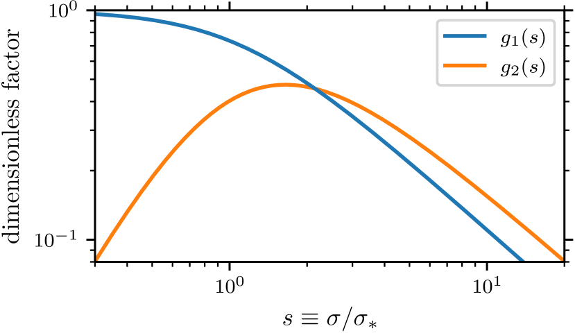
Figure 1: Dimensionless factors $g_{1}(s)$ and $g_{2}(s)$ that appear in equations (22) and (27), respectively, which are functions of the ratio $s\equiv\sigma/\sigma_{*}$ of the velocity dispersion of the perturbing matter to that of the stars. The stellar density power spectrum is proportional to $g_{1}$ (blue curve), while the stellar velocity power spectrum is proportional to $g_{2}$ (orange curve).

3.2 Velocity power

Similarly, equation (19) leads to

$$\langle\bar{v}_{i}(\bm{k})\bar{v}_{j}^{*}(\bm{k}^{\prime})\rangle =\int_{-\infty}^{t}\mathrm{d}t^{\prime}\int_{-\infty}^{t}\mathrm{d}t^{\prime\prime}\mathrm{e}^{-\frac{k^{2}\sigma_{*}^{2}}{2}(t-t^{\prime})^{2}-\frac{k^{\prime 2}\sigma_{*}^{2}}{2}(t-t^{\prime\prime})^{2}}$$

$$\hphantom{=}\times\left[\delta_{ii^{\prime}}\!-\!k_{i}k_{i^{\prime}}\sigma_{*}^{2}(t\!-\!t^{\prime})^{2}\right]\left[\delta_{\!j\!j^{\prime}}\!-\!k^{\prime}_{\!j}k^{\prime}_{\!j^{\prime}}\sigma_{*}^{2}(t\!-\!t^{\prime\prime})^{2}\right]$$

$$\hphantom{=}\times\langle a_{i^{\prime}}(\bm{k},t^{\prime})a_{j^{\prime}}(\bm{k}^{\prime},t^{\prime\prime})\rangle,$$ (25)

where repeated indices are summed. By defining $\langle\bar{v}_{i}(\bm{k})\bar{v}_{j}^{*}(\bm{k}^{\prime})\rangle\equiv(2\pi)^{3}\delta_{D}^{3}(\bm{k}-\bm{k}^{\prime})P_{v_{i}v_{j}}(\bm{k})$ and substituting equation (2), we obtain the power spectrum of mean stellar velocities,

$$P_{v_{i}v_{j}}(\bm{k}) =16\pi^{2}G^{2}\frac{k_{i}k_{\!j}}{k^{4}}P_{\rho}(k)\int_{-\infty}^{t}\mathrm{d}t^{\prime}\int_{-\infty}^{t}\mathrm{d}t^{\prime\prime}$$

$$\hphantom{=}\times\left[1\!-\!k^{2}\sigma_{*}^{2}(t\!-\!t^{\prime})^{2}\right]\left[1\!-\!k^{2}\sigma_{*}^{2}(t\!-\!t^{\prime\prime})^{2}\right]$$

$$\hphantom{=}\times\mathrm{e}^{-\frac{k^{2}\sigma_{*}^{2}}{2}\left[(t-t^{\prime})^{2}+(t-t^{\prime\prime})^{2}\right]}\mathrm{e}^{-\frac{1}{2}k^{2}\sigma^{2}(t^{\prime}-t^{\prime\prime})^{2}}$$ (26)

$$=16\pi^{2}g_{2}(\sigma/\sigma_{*})\frac{G^{2}k_{i}k_{\!j}P_{\rho}(k)}{\sigma_{*}^{2}k^{6}},$$ (27)

where we define another dimensionless function

$$g_{2}(s) \equiv\int_{0}^{\infty}\!\!\!\!\!\mathrm{d}\chi\!\!\int_{0}^{\infty}\!\!\!\!\!\mathrm{d}\xi\,(1\!-\!\chi^{2})(1\!-\!\xi^{2})\,\mathrm{e}^{-\frac{1}{2}(\chi^{2}+\xi^{2})-\frac{s^{2}}{2}(\xi-\chi)^{2}}$$ (28)

$$=\frac{s^{2}(1-s^{2})}{(1+2s^{2})^{2}(1+s^{2})}+\frac{3s^{4}[\pi-\arctan(\sqrt{1+2s^{2}}/s^{2})]}{(1+2s^{2})^{5/2}}.$$ (29)

We plot $g_{2}$ in figure 1. If the stars and the perturbing matter have the same velocity distribution, then $g_{2}$ evaluates to $g_{2}(1)=2\pi/3^{5/2}\simeq 0.40$. In the opposite limit that the stellar distribution is cold ($\sigma_{*}\ll\sigma$), $g_{2}(\sigma/\sigma_{*})\to(3\pi/2^{5/2})\sigma_{*}/\sigma$, so that $P_{v_{i}v_{j}}\propto(\sigma\sigma_{*})^{-1}$.

3.3 Density-velocity cross-correlations

Finally, we note that the cross power between the stellar density contrast and the mean velocity of stars vanishes. In particular, equations (17) and (19) imply

$$\langle\delta_{*}(\bm{k})\bar{v}_{i}^{*}(\bm{k}^{\prime})\rangle =-\mathrm{i}k_{j}\!\!\int_{-\infty}^{t}\!\!\!\!\mathrm{d}t^{\prime}\!\!\int_{-\infty}^{t}\!\!\!\!\mathrm{d}t^{\prime\prime}(t\!-\!t^{\prime})\left[\delta_{ii^{\prime}}-k^{\prime}_{i}k^{\prime}_{i^{\prime}}\sigma_{*}^{2}(t\!-\!t^{\prime\prime})^{2}\right]$$

$$\hphantom{=}\times\mathrm{e}^{-\frac{k^{2}\sigma_{*}^{2}}{2}(t-t^{\prime})^{2}-\frac{k^{\prime 2}\sigma_{*}^{2}}{2}(t-t^{\prime\prime})^{2}}$$

$$\hphantom{=}\times\langle a_{j}(\bm{k},t^{\prime})a^{*}_{i^{\prime}}(\bm{k}^{\prime},t^{\prime\prime})\rangle$$ (30)

$$=-16\pi^{2}\mathrm{i}\frac{G^{2}k_{i}P_{\rho}(k)}{\sigma_{*}^{3}k^{5}}(2\pi)^{3}\delta_{D}^{3}(\bm{k}-\bm{k}^{\prime})$$

$$\hphantom{=}\times\!\!\int_{0}^{\infty}\!\!\!\!\!\mathrm{d}\chi\!\!\int_{0}^{\infty}\!\!\!\!\!\mathrm{d}\xi\,\chi(1\!-\!\xi^{2})\mathrm{e}^{-\frac{1}{2}(\chi^{2}+\xi^{2})-\frac{(\sigma/\sigma_{*})^{2}}{2}(\xi-\chi)^{2}}$$ (31)

$$=0,$$ (32)

where the last line comes from evaluating the integrals.

4 Discussion

We derived analytic relationships between the two-point statistics of a gravitationally perturbed stellar system and those of the matter that sources the perturbations. Although the description is general, the motivation for this work was to explore the degree to which stellar systems can be used as a probe of dark matter substructures. The key results are equation (22), which describes the stellar density field, and equation (27), which describes the stellar velocity field. In both cases, the power spectrum of the stars is proportional to that of the perturbers, albeit weighted by $k^{-4}$. We also point out that the stellar density and velocity fields are completely uncorrelated with each other.

These results can be used to straightforwardly evaluate the suitability of a stellar system for probing dark matter substructure. As an example, we note that the Milky Way’s stellar halo at a radius of about $20$ kpc has a number density of order $\bar{n}_{*}\sim 10^{-5}$ pc^-3, based on a power-law density profile with index -3.5 and local normalization of about $10^{-4}$ M_⊙ pc^-3 (Helmi, 2008) and assuming the average star weighs 0.5 M_⊙. The power spectrum of the Poisson noise is hence $P_{*}(k)=\bar{n}_{*}^{-1}\sim 10^{-4}$ kpc³. The radial velocity dispersion is about 120 km s^-1 (Helmi, 2008), and if we approximate that it is isotropic and the same for stars and substructures, equation (22) implies that perturber power spectra larger than $P_{\rho}(k)\sim 10^{13}(k/\text{kpc}^{-1})^{4}$ M${}_{\odot}^{2}\,$kpc^-3 produce stellar density perturbations that exceed the level of the Poisson noise. Figure 2 shows this sensitivity limit. For comparison, we also show the nonlinear power spectrum that corresponds (per equations 9 and 10) to the subhalo model used by Bovy et al. (2017) and Delos & Schmidt (2022) to study perturbations to stellar streams at a comparable Galactocentric radius. This subhalo model is based on the numerical simulation of Diemand et al. (2008) of a Milky Way–like dark matter halo. Apparently, for $k\lesssim 0.4$ kpc^-1, this substructure model would induce perturbations in the stellar distribution that exceed the level of the Poisson noise.

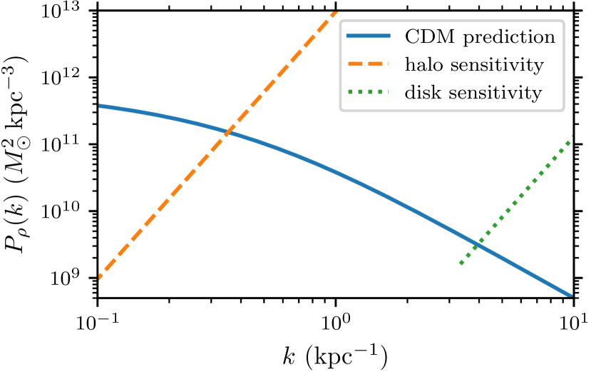
Figure 2: Testing the capacity of the Milky Way’s stellar halo and disk to probe dark matter substructure. We plot the nonlinear matter power spectrum $P_{\rho}(k)$; the solid curve shows the prediction for cold dark matter (CDM) while the dashed and dotted curves show the sensitivity limits for the Milky Way’s stellar halo at $\sim 20$ kpc and local disk stars, respectively. Specifically, for each wave number $k$, the sensitivity limit corresponds to the smallest value of $P_{\rho}(k)$ that would induce fluctuations in the stellar density field that exceed the level of the intrinsic Poisson noise arising from the finite number of stars. The predicted matter power spectrum corresponds to the subhalo model used by Bovy et al. (2017) and Delos & Schmidt (2022), which is based on the CDM simulation of Diemand et al. (2008).

A potential complication is that the stellar halo already exhibits some degree of clustering due to its history, since it is believed to consist of debris from tidally disrupted objects (Naidu et al., 2020). We remark, however, that historical clustering can be distinguished in principle from clustering associated with the gravitational perturbations discussed in this work. When clustering arises from history, density and velocity perturbations must be strongly correlated; otherwise they would rapidly dissipate. On the other hand, we showed that the transient density and velocity perturbations induced by substructure are completely uncorrelated.

The principal approximations made in these calculations are that the perturbing matter fields are the only source of gravitational acceleration and that the unperturbed systems are spatially uniform. Stars, of course, reside inside galaxies, and we have neglected the host galaxy’s gravity and its overall density structure. These approximations are valid under the following conditions.

1. The time scale $(k\sigma_{*})^{-1}$ for the stellar velocity dispersion to erase perturbations is much shorter than the stars’ orbital time scale. If perturbations can persist over an orbital period, then one cannot neglect orbital dynamics.

2. The length scale $k^{-1}$ under consideration is much smaller than the overall size of the system. Otherwise, the global structure of the system must be accounted for.

In practice, these requirements mean that the stars must comprise a velocity-dispersion-supported structure, as opposed to one supported by rotation. Hence, the calculations in this work are applicable to spheroidal galaxies, spheroidal components of galaxies, and globular star clusters. The calculations only directly apply to galactic disks or stellar streams if $k^{-1}$ is much smaller than the system’s transverse size (set by the velocity dispersion), although for larger scales, one can modify the description to include an approximate account of orbital dynamics (see Delos & Schmidt, 2022).

Based on these considerations, figure 2 also shows the estimated sensitivity of nearby stars in the Galactic disk to perturbations by substructure, plotted only up to $k^{-1}=0.3$ kpc, which is approximately the vertical scale height of the dominant component of the disk (Bland-Hawthorn & Gerhard, 2016). We assume the stars comprise a mass density of about $0.04$ M${}_{\odot}\,$pc^-3 and have a velocity dispersion of 30 km s^-1 per dimension (Bland-Hawthorn & Gerhard, 2016), and we again assume that stars have average mass 0.5 M_⊙ and that the substructure velocity dispersion is 120 km s^-1 per dimension. Figure 2 suggests that dark substructure around $k\sim 4$ kpc^-1 could be barely detectable through induced density perturbations of the local stellar field. However, it should be noted that substructure that crosses the disk is likely disrupted to a significantly greater degree than is reflected in the dark-matter-only simulation on which the predicted $P_{\rho}(k)$ in figure 2 is based (e.g. D’Onghia et al., 2010). Also, the disk sensitivity prediction is based on equation (22), which is derived under the assumption that the stars and the substructure have the same rest frame. As we discuss in section 2, the net motion between the stars and the substructure would alter the result for wave vectors $\bm{k}$ not perpendicular to it. A third concern is that the calculations in this work neglect the self-gravity of the stellar perturbations themselves, which can be relevant for galactic disks (e.g. Widrow, 2023).

A final note is that we only studied two-point statistics. Nonlinear dark matter structures can be highly nongaussian, and the resulting stellar density and velocity fields would have significantly nongaussian statistics as a result. However, it is possible to analytically evaluate higher-order statistics through similar calculations to those presented in this work.

Data Availability

No new data were generated or analysed in support of this research.

References

- Amorisco et al. (2016) Amorisco N. C., Gómez F. A., Vegetti S., White S. D. M., 2016, MNRAS, 463, L17
- Banik & Bovy (2019) Banik N., Bovy J., 2019, MNRAS, 484, 2009
- Banik et al. (2018) Banik N., Bertone G., Bovy J., Bozorgnia N., 2018, J. Cosmology Astropart. Phys., 2018, 061
- Banik et al. (2021a) Banik N., Bovy J., Bertone G., Erkal D., de Boer T. J. L., 2021a, MNRAS, 502, 2364
- Banik et al. (2021b) Banik N., Bovy J., Bertone G., Erkal D., de Boer T. J. L., 2021b, J. Cosmology Astropart. Phys., 2021, 043
- Bazarov et al. (2022) Bazarov A., Benito M., Hütsi G., Kipper R., Pata J., Põder S., 2022, Astronomy and Computing, 41, 100667
- Bland-Hawthorn & Gerhard (2016) Bland-Hawthorn J., Gerhard O., 2016, ARA&A, 54, 529
- De Boer et al. (2020) De Boer T. J. L., Erkal D., Gieles M., 2020, MNRAS, 494, 5315
- Bonaca et al. (2019) Bonaca A., Hogg D. W., Price-Whelan A. M., Conroy C., 2019, ApJ, 880, 38
- Bovy et al. (2017) Bovy J., Erkal D., Sanders J. L., 2017, MNRAS, 466, 628
- Capuzzo Dolcetta et al. (2005) Capuzzo Dolcetta R., Di Matteo P., Miocchi P., 2005, AJ, 129, 1906
- Carlberg (2009) Carlberg R. G., 2009, ApJ, 705, L223
- Carlberg (2012) Carlberg R. G., 2012, ApJ, 748, 20
- Carlberg (2016) Carlberg R. G., 2016, ApJ, 820, 45
- Carlberg & Agler (2023) Carlberg R. G., Agler H., 2023, The Astrophysical Journal, 953, 99
- Chequers et al. (2018) Chequers M. H., Widrow L. M., Darling K., 2018, MNRAS, 480, 4244
- D’Onghia et al. (2010) D’Onghia E., Springel V., Hernquist L., Keres D., 2010, ApJ, 709, 1138
- Davies et al. (2023) Davies E. Y., Vasiliev E., Belokurov V., Evans N. W., Dillamore A. M., 2023, MNRAS, 519, 530
- Delos & Schmidt (2022) Delos M. S., Schmidt F., 2022, MNRAS, 513, 3682
- Diemand et al. (2008) Diemand J., Kuhlen M., Madau P., Zemp M., Moore B., Potter D., Stadel J., 2008, Nature, 454, 735
- Doke & Hattori (2022) Doke Y., Hattori K., 2022, ApJ, 941, 129
- Erkal & Belokurov (2015) Erkal D., Belokurov V., 2015, MNRAS, 454, 3542
- Erkal et al. (2016) Erkal D., Belokurov V., Bovy J., Sanders J. L., 2016, MNRAS, 463, 102
- Ferguson et al. (2022) Ferguson P. S., et al., 2022, AJ, 163, 18
- González-Morales et al. (2013) González-Morales A. X., Valenzuela O., Aguilar L. A., 2013, J. Cosmology Astropart. Phys., 2013, 001
- Helmi (2008) Helmi A., 2008, A&ARv, 15, 145
- Ibata et al. (2002) Ibata R. A., Lewis G. F., Irwin M. J., Quinn T., 2002, MNRAS, 332, 915
- Ibata et al. (2020) Ibata R., Thomas G., Famaey B., Malhan K., Martin N., Monari G., 2020, ApJ, 891, 161
- Johnston et al. (2002) Johnston K. V., Spergel D. N., Haydn C., 2002, ApJ, 570, 656
- Koppelman & Helmi (2021) Koppelman H. H., Helmi A., 2021, A&A, 649, A55
- Küpper et al. (2008) Küpper A. H. W., MacLeod A., Heggie D. C., 2008, MNRAS, 387, 1248
- Küpper et al. (2010) Küpper A. H. W., Kroupa P., Baumgardt H., Heggie D. C., 2010, MNRAS, 401, 105
- Küpper et al. (2012) Küpper A. H. W., Lane R. R., Heggie D. C., 2012, MNRAS, 420, 2700
- Li et al. (2021) Li T. S., et al., 2021, ApJ, 911, 149
- Malhan et al. (2021) Malhan K., Valluri M., Freese K., 2021, MNRAS, 501, 179
- Montanari & García-Bellido (2022) Montanari F., García-Bellido J., 2022, Physics of the Dark Universe, 35, 100978
- Naidu et al. (2020) Naidu R. P., Conroy C., Bonaca A., Johnson B. D., Ting Y.-S., Caldwell N., Zaritsky D., Cargile P. A., 2020, ApJ, 901, 48
- Ngan & Carlberg (2014) Ngan W. H. W., Carlberg R. G., 2014, ApJ, 788, 181
- Peñarrubia (2019) Peñarrubia J., 2019, MNRAS, 484, 5409
- Pearson et al. (2017) Pearson S., Price-Whelan A. M., Johnston K. V., 2017, Nature Astronomy, 1, 633
- Penarrubia et al. (2010) Penarrubia J., Koposov S. E., Walker M. G., Gilmore G., Wyn Evans N., Mackay C. D., 2010, arXiv e-prints, p. arXiv:1005.5388
- Qian et al. (2022) Qian Y., Arshad Y., Bovy J., 2022, MNRAS, 511, 2339
- Ramirez & Buckley (2023) Ramirez E. D., Buckley M. R., 2023, MNRAS, 525, 5813
- Sanders et al. (2016) Sanders J. L., Bovy J., Erkal D., 2016, MNRAS, 457, 3817
- Scherrer & Bertschinger (1991) Scherrer R. J., Bertschinger E., 1991, ApJ, 381, 349
- Siegal-Gaskins & Valluri (2008) Siegal-Gaskins J. M., Valluri M., 2008, ApJ, 681, 40
- Starkenburg & Helmi (2015) Starkenburg T. K., Helmi A., 2015, A&A, 575, A59
- Tavangar et al. (2022) Tavangar K., et al., 2022, ApJ, 925, 118
- Tremaine et al. (2023) Tremaine S., Frankel N., Bovy J., 2023, MNRAS, 521, 114
- Weatherford et al. (2023) Weatherford N. C., Rasio F. A., Chatterjee S., Fragione G., Kıroğlu F., Kremer K., 2023, arXiv e-prints, p. arXiv:2310.01485
- Webb et al. (2019) Webb J. J., Bovy J., Carlberg R. G., Gieles M., 2019, MNRAS, 488, 5748
- Widrow (2023) Widrow L. M., 2023, MNRAS, 522, 477
- Yoon et al. (2011) Yoon J. H., Johnston K. V., Hogg D. W., 2011, ApJ, 731, 58