Deep Hybrid Camera Deblurring

Abstract

Mobile cameras, despite their significant advancements, still face low-light challenges due to compact sensors and lenses, leading to longer exposures and motion blur. Traditional solutions like blind deconvolution and learning-based methods often fall short in handling ill-posedness of the deblurring problem. To address this, we propose a novel deblurring framework for multi-camera smartphones, utilizing a hybrid imaging technique. We simultaneously capture a long exposure wide-angle image and ultra-wide burst images from a smartphone, and use the sharp burst to estimate blur kernels for deblurring the wide-angle image. For learning and evaluation of our network, we introduce the HCBlur dataset, which includes pairs of blurry wide-angle and sharp ultra-wide burst images, and their sharp wide-angle counterparts. We extensively evaluate our method, and the result shows the state-of-the-art quality.

1 Introduction

While mobile cameras have significantly improved, they still struggle in low-light environment due to their small sensors and lenses, leading to longer exposure times and increased susceptibility to motion blur from hand movement or moving subjects. To remove blur, numerous learning-based deblurring methods have been proposed [28, 40, 21, 22, 47, 44, 48, 11, 7, 8], which train deep networks on deblurring datasets. Nonetheless, their performances are still limited due to the wide variety of blur patterns in real-world blurred images that makes it difficult for the network to encompass all potential blur degradation [19].

To address the aforementioned challenges, several deep learning-based methods have been proposed, focusing on blur kernel estimation [5, 6, 36, 19, 16]. These methods train kernel estimation networks that are leveraged for the deblurring process, enhancing both their generalization ability and performance [19, 16]. However, these approaches rely on synthetic blur kernel datasets derived from restrictive blur models for training, such as linear motion [36], uniform blur [19, 6], segmented uniform blur [5], which cannot reflect realistic blur trajectories. Additionally, estimating blur kernels from a single blurry image is inherently challenging. The infinite number of blur kernels and sharp images can result in the same blurred image, making the task a highly ill-posed problem.

In this paper, we propose a practical image deblurring framework based on blur kernels, specifically designed for modern mobile devices like the Apple iPhone and Samsung Galaxy series, which now commonly feature asymmetric multi-cameras. To facilitate accurate blur kernels estimation, we revisit hybrid imaging [2, 38, 39, 25] and design our framework to leverage images captured by multi-cameras with different setting, leading to improvement in overall deblurring quality.

The core concept of hybrid imaging, initially introduced by Ben-Ezra and Nayar [2], is centered on capturing images from multi-cameras and selectively extracting advantageous features of each image derived from its distinct camera setting, such as shutter speed and focal length, to compose a final enhanced image. Modern mobile devices with asymmetric multi-cameras naturally align with this concept. These devices typically have at least two cameras with different but fixed focal lengths, offering varying camera settings between the cameras. In dual-camera setup, the wide-angle camera has higher focal length and captures subjects in higher resolution with narrower field of view (FOV) compared to its counterpart, typically the ultra-wide camera.

Our framework leverages multi-cameras in mobile devices for hybrid imaging by customizing capture settings of the cameras, to address the challenges posed by previous deblurring approaches in blur kernel estimation primarily stemming from ambiguities in estimating blur kernels using only a single blurry image. Specifically, our multi-camera hybrid imaging utilizes the wide-angle and ultra-wide cameras on iPhone 13 Pro Max as the primary and secondary components within the hybrid imaging system, respectively, with the wide-angle image as our target.

In our dual-camera hybrid imaging system, the main wide-angle camera, with a higher focal length, captures high-resolution images at a slow shutter speed. This setup, while offering superior image quality such as less noise and accurate color representation, is prone to motion blur. Meanwhile, the secondary ultra-wide camera captures a burst of lower-resolution images at rapid shutter speed, ensuring sharpness but with potentially reduced image quality. The key concept here is to use the sharp ultra-wide images, captured with a short exposure time, to accurately gather motion information which is difficult to obtain from the blurry wide-angle images alone. This motion information is then utilized to deblur the wide-angle image, thus retaining the image quality benefits of its camera setting.

For the kernel-based motion deblurring, we introduce a deep network with two sub-networks: the Hybrid Camera Deblurring Network (HC-DNet) and the Fusion Network (HC-FNet). These networks deblur blurry wide-angle images by leveraging the strengths of our dual-camera hybrid imaging system. HC-DNet uses a burst of sharp ultra-wide images to compute optical flows and transform them to per-pixel blur kernels for deblurring the wide-angle image. However, challenges may arise in blur kernels due to errors in the optical flows, particularly in textureless regions and small objects. To mitigate this, HC-FNet, inspired by burst imaging techniques [3, 13, 27], refines the output of HC-DNet using the entire sequence of ultra-wide burst images to compensates for any residual blurs or kernel estimation errors from HC-DNet.

To train and evaluate our model, we present the HCBlur dataset, created using videos of the wide-angle and ultra-wide cameras. We developed a hybrid camera iOS application to enable simultaneous video capture from these cameras. We gathered 1,176 pairs of wide-angle and ultra-wide videos, then synthesized blurred images by averaging sharp frames of wide-angle videos. The HCBlur dataset comprises 8,568 pairs of blurry wide-angle images with corresponding sets of sharp ultra-wide burst images, reflecting our multi-camera hybrid imaging setup, along with their corresponding sharp wide-angle ground-truth images.

To summarize, our contributions include:

• the first deblurring framework designed for mobile devices with multi-cameras leveraging hybrid imaging.

• a novel deep networks for wide-angle image deblurring using ultra-wide burst images in blur kernel estimation and detail compensation.

• the HCBlur dataset, the first dataset for motion deblurring training with hybrid imaging.

2 Related Work

Image Deblurring  To restore a sharp image from a blurred one, deblurring has been widely studied. Conventional blind deconvolution methods [17, 33, 9, 45, 46, 30, 37, 10] employ an iterative process to optimize a blur kernel and a latent sharp image. Recently, learning-based deblurring methods [28, 40, 21, 22, 47, 44, 48, 11, 7, 8] directly estimate the latent sharp image. However, these methods still struggle with the generalization problem due to the difficulty of learning arbitrary possible motion blur [16].

Blur Kernel Estimation  Various blur kernel estimation methods have been proposed such as edge-based [37, 9], tho-phase kernel estimation [45], phase-only image [31], MAP-based [10, 46], $L_{0}$ norm prior [46]. There are a few learning-based blur kernel estimation methods [5, 6, 36, 19, 16]. They proposed blur kernel estimation networks for distinct types of blur such as uniform blur [6, 19], linear motion [36], non-uniform blur [5, 16]. The blur kernel is exploited by non-blind deconvolution [5, 6, 36] or conditioning for deblurring networks [19, 16]. However, their performance is still limited due to the ill-posedness of the deblurring problem.

Hybrid Imaging Deblurring  Ben-Ezra and Nayar [2] first introduced a deblurring method using hybrid imaging. Tai et al. [38, 39] extends the idea for non-uniform deblurring and video deblurring. Li et al. [25] proposed a method of hybrid imaging for motion deblurring and depth map super-resolution. We introduce a hybrid imaging deblurring method for real-world mobile devices, addressing the challenges of different FOVs of cameras, which is more practical and highly relevant to real-world scenarios.

Burst Enhancement Burst enhancement networks [3, 13, 14, 27] for super-resolution take low-resolution burst images as inputs and enhance their image quality. Bhat et al. [3] proposed a method that aligns burst images using optical flow and merges them using attention-based methods. For the alignment of burst images, implicit alignment using deformable convolution is adopted by [13, 14, 27]. Mehta et al. [27] proposed merging of burst images using transposed attention. The HC-FNet also uses burst images, but its primary objective is deblurring rather than the super-resolution of low-resolution images.

Face Deblurring using Dual Cameras  Lai et al. [23] proposed a face deblurring method that leverages dual cameras of smartphone cameras. They capture a blurred image and a short-exposure image simultaneously and align the short-exposure image using an optical flow network. Then, a UNet conducts the deblurring using concatenated two images. The method is designed specifically for face deblurring based on utilizing an image. On the other hand, our method is for general deblurring using burst images.

3 Hybrid Imaging for Mobile Multi-Cameras

In our proposed hybrid imaging system, we use wide-angle and ultra-wide cameras of the iPhone 13 Pro Max. These cameras simultaneously capture a scene at different temporal and spatial resolutions. Here, our goal is to enhance a potentially blurry wide-angle images, typically captured at slow shutter speeds, by leveraging a burst of sharp ultra-wide images. This setting allows our deblurring framework to address motion blur and improve overall image quality in challenging low-light scenarios. Throughout the rest of the paper, for brevity, we denote wide-angle image and the ultra-wide burst images as $\mathbf{W}$ and $\mathbf{UWs}$, respectively.

To establish differing frame capture rates between the two cameras, we develop a hybrid camera iOS application using the multi-camera API [1]. Our hybrid camera application sets the wide-angle camera to capture a long-exposure image $\mathbf{W}$ at 4K resolution ($\text{2160}\!\times\!\text{3840}$), with configurable exposure times ranging from $1/15$s and $1/2$s. Simultaneously, the ultra-wide camera captures burst images $\mathbf{UWs}$, each at 60 frames per second, each with a resolution of 720P ($\text{720}\!\times\!\text{1280}$). To prevent blurs in the burst images captured by the ultra-wide camera, we limit the maximum exposure time to $1/120$s. The acquisition times of $\mathbf{W}$ and $\mathbf{UWs}$ could slightly differ because of the distinct frame rates. To this end, we record timestamps that include start and end capturing times of each image taken by both the wide-angle and ultra-wide cameras. These timestamps provide a reference to extract images of $\mathbf{UWs}$ corresponding to the $\mathbf{W}$and allow us to estimate temporally synchronized blur kernels with the actual exposure of $\mathbf{W}$.

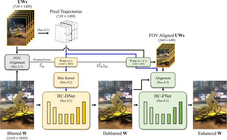
Figure 1: The overview of the proposed method.

3.1 FOV Alignment

While our hybrid camera application is capable of concurrent capturing of a wide-angle image $\mathbf{W}$ and ultra-wide bursts $\mathbf{UWs}$, additional processing is required to mitigate geometric misalignment between $\mathbf{W}$ and $\mathbf{UWs}$, which arises from differences in physical properties in the multi-cameras. Specifically, the baseline of two cameras and different focal lengths cause scene-dependent disparities and different FOV between the captured images, respectively.

However, in our hybrid imaging setup where the wide-angle camera configured for long exposure, the potential presence of blur in $\mathbf{W}$ can introduce errors when naïvely applying conventional alignment methods [26, 15]. To address these issues, we introduce FOV alignment, a technique for aligning multi-camera images based on stereo calibration [50] and plane sweep methods [12]. Our FOV alignment module is designed to preserve the spatial coherency of ultra-wide images by considering a constraining planar depth plane and utilizing stereo camera parameters during alignment, resulting in robust alignment. Moreover, our FOV alignment module extends beyond previous mobile multi-camera alignment method, which only account for differences in focal lengths and crop wider FOV images to match narrower ones [23, 42, 24]. Instead, our alignment module considers scene-dependent disparities between multi-camera images, further enhancing alignment accuracy.

Our FOV alignment aims at determining a transform index $\hat{C}_{w}$ containing per-pixel offsets that resample ultra-wide images in a way that maximizes their similarity with the wide-angle image $\mathbf{W}$. Mathematically, we have:

$$\hat{C}_{w}=\mathop{\mathrm{argmin}}\limits_{T(C_{w},d|d\in D)}MSE(I^{w},\mathbb{W}(I^{uw},T(C_{w},d))$$ (1)

where $T(C_{w},d)=K_{uw}E_{r}^{-1}dK_{w}^{-1}C_{w}$. Here, $C_{w}$ represents a meshgrid containing 2D coordinates of a wide-angle image, and our goal is to find a transform index $T({C}_{w},d)$, where $T$ transforms ${C}_{w}$ based on a planar depth value $d$ chosen from candidates in $D$, which includes 18 candidate depth values derived from pixel disparities ranging from 5 to 95 with a 5-pixel interval. To compute a transformed coordinates in $T(\cdot)$, we use intrinsic matrices $K_{w}$ and $K_{uw}$ of wide-angle and ultra-wide cameras, respectively, and a relative extrinsic matrix $E_{r}$ obtained from stereo calibration.

We choose the optimal transform index $\hat{C}_{w}$ from a set of 18 candidates ${T({C}_{w},d|d\in D)}$ by minimizing the mean-squared-error (MSE) between the wide-angle frame $I^{w}$ and an ultra-wide frame $I^{uw}$ resampled using bilinear sampling operation denoted as $\mathbb{W}$ with each candidate. Note that for $I^{uw}$, we use an averaged image created from burst ultra-wide images in $\mathbf{UWs}$, to include blurs closely resembles the blurs in $\mathbf{W}$, facilitating a more meaningful comparison between resampled ultra-wide and wide-angle images. The result of our FOV alignment is the transform index $\hat{C}_{w}$, which is then employed by our deblurring networks for them to utilize information in the burst of ultra-wide images $\mathbf{UWs}$ while deblurring the wide-angle image $\mathbf{W}$.

4 Deep Hybrid Camera Deblurring

In this section, we introduce the deblurring network, designed to leverage our hybrid imaging setup (Fig. 1). Our deblurring network comprises two sub-networks: hybrid-camera deblurring network (HC-DNet) and fusion network (HC-FNet). Leveraging wide-angle blurry image $\mathbf{W}$ and a burst of ultra-wide angle images $\mathbf{UWs}$, our network aims to enhance $\mathbf{W}$ by utilizing $\mathbf{UWs}$. HC-DNet takes the lead in deblurring $\mathbf{W}$, and the output is then refined by HC-FNet to achieve further enhancement. The two sub-networks differ in how they extract and apply useful information of $\mathbf{UWs}$ when processing $\mathbf{W}$.

HC-DNet leverages $\mathbf{UWs}$ to construct per-pixel blur kernels aligned with $\mathbf{W}$. To construct the blur kernels, we first compute a optical flow-based pixel trajectories within $\mathbf{UWs}$, containing per-pixel motion information its center frame to each of other frames. Then, the pixel trajectories are transformed into per-pixel blur kernels and aligned to $\mathbf{W}$ using the FOV alignment module. The HC-DNet subsequently performs deblurring on $\mathbf{W}$ by exploiting the constructed blur kernels. However, errors may arise during the constructions of the blur kernels, particularly for regions lacking textures or containing small objects, potentially leading to inaccuracies in the optical flow estimation.

HC-FNet utilizes $\mathbf{UWs}$ to provide additional compensation to address potential errors in the deblurring process, especially those caused by inaccurate blur kernels. To this end, we design HC-FNet to directly utilize $\mathbf{UWs}$ and leverage useful information that can be extracted from the burst images. HC-FNet takes deblurred resulf of HC-DNet and produces the final output further enhanced by fusing the burst information of $\mathbf{UWs}$.

4.1 Pixel Trajectories in UWs

Before delving into the specifics of HC-DNet and HC-FNet, we first explain how we compute the pixel trajectories from the burst of ultra-wide images $\mathbf{UWs}$, as this process is utilized by both sub-networks for constructing blur kernels and extracting aggregated burst information.

To compute pixel trajectory of $\mathbf{UWs}$, consisting of frames $\{I^{uw}_{1},\cdots,I^{uw}_{c},\cdots,I^{uw}_{e}\}$, where 1, $c$ and $e$ indicate the first, center, and last frame indices respectively, we begin by estimating backward and forward optical flows across the adjacent image pairs from each 1st and last frame towards the center frame. Specifically, for all adjacent frames from the 1st to ($c-1$)-th index, we compute backward optical flow as $B^{i+1}_{i}=RAFT(I^{uw}_{i+1},I^{uw}_{i})$, where $RAFT$ is the optical flow estimation network [41]. For the remaining frames from $(c+1)$-th to $e$-th index, we compute forward optical flows as $F^{i-1}_{i}=RAFT(I^{uw}_{i-1},I^{uw}_{i})$.

Having estimated flows $\{B^{2}_{1}\dots B^{c}_{c-1},F^{c}_{c+1}\dots F^{e-1}_{e}\}$, we construct pixel trajectory denoted as $P^{c}$. The pixel trajectory $P^{c}$ essentially represents the per-pixel trajectories of each pixel in a center frame towards the other frames. It is computed by cumulatively adding the estimated backward and forward optical flows in both directions, starting from the center frame. Initially, the pixel trajectory for the center frame is set with a pixel coordinate: $P^{c}_{c}(x,y)=\{x,y\}$. Then, we first compute the backward trajectory using computed backward optical flows as follows:

$$P^{c}_{i}(x,y)=P^{c}_{i+1}(x,y)+B^{i+1}_{i}(P^{c}_{i+1}(x,y))$$ (2)

where $\forall i\in\{c-1,\dots,1\}$ and $P^{c}_{i}(x,y)$ represents the coordinates of a pixel at $(x,y)$ in the center frame to $i$-th frame. For the forward trajectories, we use forward flows computed from the center to the last frames as follows:

$$P^{c}_{i}(x,y)=P^{c}_{i-1}(x,y)+F^{i-1}_{i}(P^{c}_{i-1}(x,y))$$ (3)

where $\forall i\in\{c+1,\dots,e\}$. Finally, the pixel trajectory $P^{c}$ contains the per-pixel trajectory of a center frame of $\mathbf{UWs}$ to each other frame indices. It is subsequently utilized by HC-DNet for constructing blur kernel and by HC-FNet for aggregating burst information from $\mathbf{UWs}$.

4.2 HC-DNet

In this section, we present the HC-DNet, which constructs per-pixel blur kernels utilizing a burst of ultra-wide images $\mathbf{UWs}$ and exploits them in the process of deblurring a blurry wide-angle image $\mathbf{W}$.

Blur Kernel Construction

HC-DNet first constructs per-pixel blur kernels using $\mathbf{UWs}$. The blur kernel is constructed based on the pixel trajectory $P^{c}$ of $\mathbf{UWs}$ (Sec. 4.1), and for the final blur kernel to be geometrically aligned to $\mathbf{W}$, we first align the $P^{c}$ to $\mathbf{W}$ using the transform index $\hat{C}_{w}$ computed in the FOV alignment module (Sec. 3.1). Formally, we have:

$$\bar{P}^{c}_{i}=K_{w}E_{r}dK_{uw}^{-1}P^{c}_{i},$$ (4)

$$\hat{P}^{c}_{i}=\mathbb{W}(\bar{P}^{c}_{i},\hat{C}_{w}),$$ (5)

where, $\bar{P}^{c}_{i}$ is the pixel trajectories converted from ${P}^{c}_{i}$ to match the coordinate values with the coordinates system of the wide-angle camera. For the planar depth value $d$, we use the same value used when computing $\hat{C}_{w}$ (Eq. 1) in the FOV alignment module. Finally, $\hat{P}^{c}_{i}$ is the pixel trajectory of $\mathbf{UWs}$ geometrically aligned to $\mathbf{W}$.

Next, we construct the blur kernel directly leveraging the aligned pixel trajectories $\hat{P}^{c}$. However, $\hat{P}^{c}$ may not directly compatible to be utilized for convolutional neural network (CNN), due to potential variations in its temporal dimensions caused by the varying number of burst images in $\mathbf{UWs}$, which depends on the camera settings. To adapt $\hat{P}^{c}$ for use with CNNs, we further process it to fix its temporal dimension. This involves 1D interpolation to ensure a consistent number of time stamps. With pixel trajectories ${\hat{P}_{1}^{c},\dots,\hat{P}_{e}^{c}}$ from $\mathbf{UWs}$ and their timestamps ${t_{1},\dots,t_{e}}$, where $t_{1}$ and $t_{e}$ correspond to the start and end capture timestamps of $\mathbf{W}$, we construct the blur kernel $K$ as follows:

$$K_{t} =(t-t_{i})\cdot\frac{\hat{P}^{c}_{i+1}-\hat{P}^{c}_{i}}{t_{i+1}-t_{i}}+\hat{P}^{c}_{i},$$ (6)

where $\forall t\in\{0,0.125,\dots,0.875,1\}$ is the pre-defined fixed time stamps. $t_{i+1}$ and $t_{i}$ are the nearest relative time stamps of $\mathbf{UWs}$ with respect to each $t$. For the final blur kernel $K$, we subtract the values of $K_{0.5}$ from all $K_{i}$ to represent the relative distance to the center, which are then concatenated along the channel dimension for input to the network.

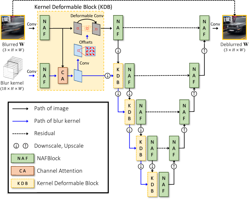
Figure 2: Architecture of the HC-DNet.

Architecture

HC-DNet takes a blurred $\mathbf{W}$ and a blur kernel $K$ as inputs to produce deblurred $\mathbf{W}$ as the output (Fig. 2). The network follows the U-Net architecture, in which we compose each level of encoder and decoder blocks with NAFBlocks [8]. To optimize the utilization of the blur kernel $K$, we design a novel kernel deformable block (KDB), which we attach before each level of the encoders. KDB is specifically designed to promote adaptive processing of $\mathbf{W}$ depending on blur kernel $K$, for facilitating the utilization of $\mathbf{UWs}$. In KDB, features of $\mathbf{W}$ and $K$ are initially extracted by NAFBlocks. Channel attentions [18] are then computed from the features of $\mathbf{W}$ that are attended on features of blur kernels, which is to prevent utilization of potentially inaccurate blur kernels. Subsequently, the attended features of $K$ are used for predicting offsets and weights for a deformable convolution layer [51], which adaptively handles features of $\mathbf{W}$ depend on $K$, leading to more effective utilization of $K$ in deblurring $\mathbf{W}$.

4.3 HC-FNet

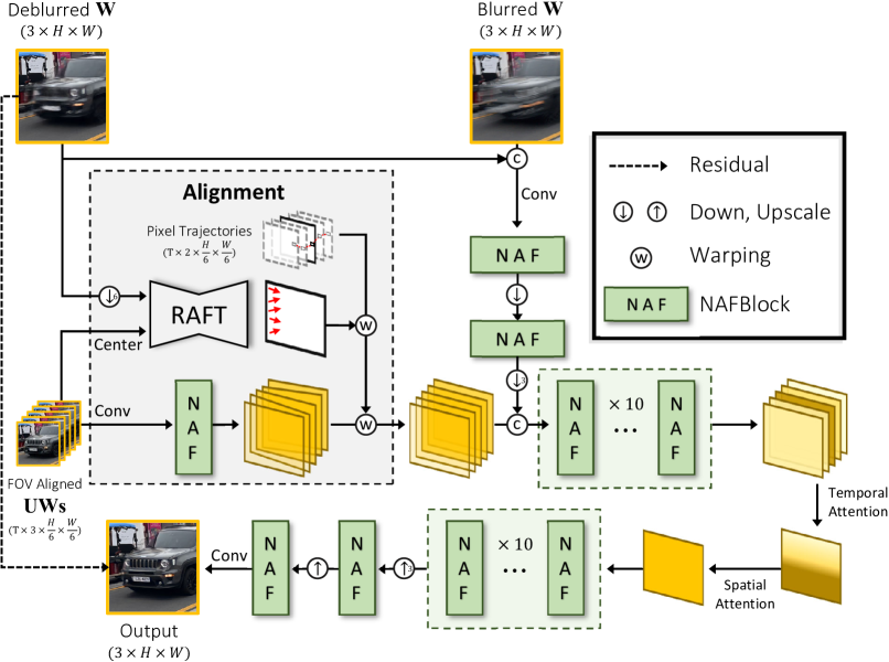
Figure 3: Architecture of the HC-FNet.

While HC-DNet employs a blur kernel constructed from the burst of ultra-wide images $\mathbf{UWs}$ to deblur $\mathbf{W}$, potential errors may still persist in the deblurred result, especially if there are inaccuracies in the optical flow estimation during the construction of blur kernels. To mitigate these remaining errors in the deblurring process, HC-FNet leverages $\mathbf{UWs}$ as an additional source of compensation. Inspired by the burst enhancement network [3], we design HC-FNet to incorporate $\mathbf{UWs}$ and extract useful information that can be derived from the burst images to be fused and further enhance the quality of the deblurred image.

HC-FNet takes a wide-angle image $\mathbf{W}$ deblurred by HC-DNet and ultra-wide burst images $\mathbf{UWs}$ as inputs to produce the final enhanced output. For effective extraction and fusion of the burst images, accurate per-pixel alignment of each ultra-wide image in the burst of $\mathbf{UWs}$ to the deblurred wide-angle image is required. To achieve this, HC-FNet incorporates FOV alignment (Sec. 3.1) on $\mathbf{UWs}$ and additionally applies per-pixel alignment between each frame in $\mathbf{UWs}$ and the deblurred $\mathbf{W}$ leveraging pixel trajectories (Sec. 4.1). Subsequently, HC-FNet utilizes these per-pixel aligned $\mathbf{UWs}$ to further improve the quality of the deblurred image. In this section, we first explain the alignment process and then describe the architecture of HC-FNet.

Per-pixel Alignment of UWs with deblurred W  We apply resolution-preserving FOV alignment on $\mathbf{UWs}$ and its pixel trajectory $P^{c}_{i}$ to be aligned with the wide-angle image $\mathbf{W}$. Here, we use with 6$\times$ downsampled version of transform index $\hat{C}_{w}$, denoted as $(\hat{C}_{w})_{6\downarrow}$, to maintain original resolution of sampling sources. Mathematically, we have:

$$\tilde{I}^{uw}_{i}=\mathbb{W}(I^{uw}_{i},(\hat{C}_{w})_{6\downarrow})$$ (7)

$$\tilde{P}^{c}_{i}=\mathbb{W}(P^{c}_{i},(\hat{C}_{w})_{6\downarrow})$$ (8)

where $\tilde{I}^{uw}_{i}$ represents the $i$-th resolution-preserved image of the FOV-aligned $\mathbf{UWs}$, and $\tilde{P}^{c}$ is the aligned pixel trajectory with preserved resolution. Here, $(\cdot){s\downarrow}$ denotes bicubic downsampling with a scale factor $s$.

The results of resolution-preserved FOV alignment have limitations for burst information extraction. Because the transform index $\hat{C}_{w}$ is computed from planar depth, the FOV-aligned ultra-wide images in $\tilde{I}^{uw}$ may not be precisely pixel-wise aligned with the deblurred $\mathbf{W}$. Since HC-FNet processes the deblurred image, achieving a more accurate alignment of $\mathbf{UWs}$ with the deblurred $\mathbf{W}$ can boost the burst information extraction process.

To address this, we compute per-pixel warping map that can further refine the alignment of $\tilde{I}^{uw}$ with $\mathbf{W}$. Specifically, we begin by resizing the deblurred image to match the resolution of $\tilde{I}^{uw}$. Then, we estimate optical flow between the the center frame FOV aligned ultra-wide image $I_{c}^{uw}$ and deblurred image, denoted as $D^{w}$. Formally, we have:

$$\tilde{F}^{deblur}_{c}=RAFT((D^{w})_{\downarrow},\tilde{I}_{c}^{uw}),$$ (9)

where, $\tilde{F}_{c}^{deblur}$ is the motion from the deblurred image to the center frame of FOV aligned ultra-wide image $\tilde{I}_{c}^{uw}$. Using $\tilde{F}_{c}^{deblur}$ and FOV-aligned pixel trajectories $\tilde{P}^{c}_{i}$, we can compute per-pixel warping indices to apply per-pixel alignment on $\tilde{I}^{uw}_{i}$ with respect to the deblurred image. This can be defined as follows:

$$\tilde{P}^{deblur}_{i}=\mathbb{W}(\tilde{P}^{c}_{i},\tilde{F}^{deblur}_{c}),$$ (10)

where $\tilde{P}^{deblur}_{i}$ contains the coordinates representing per-pixel motion from the deblurred image to each FOV-aligned ultra-wide image $\tilde{I}^{uw}_{i}$. Finally, in HC-FNet, $\tilde{P}^{deblur}_{i}$ is utilized to apply per-pixel alignment to the intermediate feature extracted from $\tilde{I}^{uw}_{i}$.

Architecture of HC-FNet  Our HC-FNet is designed based on the architecture used in the previous burst image-based super-resolution method [3], in which low-resolution burst images are utilized to super-resolve a target low-resolution image. We increase the efficiency of the network by adopting NAFBlocks in the architecture. The network takes $\mathbf{UWs}$ and deblurred $\mathbf{W}$, as well as the original blurred $\mathbf{W}$, to preserve information that might otherwise be lost during deblurring [40]. We first apply resolution-preserving FOV alignment on each ultra-wide image in $\mathbf{UWs}$ to compute aligned burst $\tilde{I}^{uw}$, using Eq. 8. Then, HC-FNet computes features of $\tilde{I}^{uw}$ whose alignment is further refined using the per-pixel warping map $\tilde{P}^{deblur}_{i}$ computed using Eq. 10 that provides refined alignment information regarding deblurred $\mathbf{W}$. After the alignment, the features of the deblurred and blurred $\mathbf{W}$ are concatenated with the aligned features. These combined features are then fused through NAFBlocks, which first process the burst features of aligned $\mathbf{UWs}$ frame-by-frame, each of which are concatenated with blurred and deblurred features of $\mathbf{W}$. We then aggregate these burst features using the temporal and spatial attention module [43] to merge them into a single frame. Finally, the merged features are further processed by additional NAFBlocks and upscaled to the resolution of $\mathbf{W}$ through upsampling layers.

5 HCBlur Dataset

We introduce the HCBlur dataset for training the HC-DNet and HC-FNet. We simultaneously capture sharp videos of wide and ultra-wide cameras and synthesize blurred $\mathbf{W}$ by averaging the sharp frames, which is a common method for synthesizing blurred datasets [28, 29, 32, 35, 34].

We modified our hybrid camera application for simultaneously capturing videos. Specifically, the wide camera captures videos of 4K resolution at 30 frames per second, while the ultra-wide camera captures videos of 720P resolution at 60 frames per second. Using the application, we collected video pairs of wide and ultra-wide cameras in various indoor, daytime, and night-time scenes. To prevent blur in the videos, the maximum shutter speed was set to 1/240 and 1/120 seconds for daytime and night-time scenes, respectively. We recorded videos of the wide camera at 30 frames per second, due to the limitation of multi-camera API[1]. Averaging the videos can result in discontinuous blur due to the large motion between frames. To address this problem, we estimated optical flows between frames and excluded frames with a maximum displacement greater than 36 pixels. The number of frames for averaging was randomly sampled, ranging from 5 to 13, and the center frame of the frames was used as the ground truth image. To construct $\mathbf{UWs}$, frames of ultra-wide video were extracted using their timestamps. We randomly subsampled the frames from 5 to 14 to create a reasonable number of images.

We adopt a realistic blur synthesis pipeline [32], which can improve the generalization ability of a synthetic dataset for deblurring on real-world blurred images. Specifically, we applied the frame interpolation method [49] before averaging and mask-based saturation synthesis [32] to generate realistic light streaks. To simulate realistic noise, we calibrated the shot and read noise parameters of our camera system, then synthesized Poisson-Gaussian noise on blurred $\mathbf{W}$ and $\mathbf{UWs}$. In indoor or night scenes, the frames of ultra-wide videos already contain significant noise, so we skipped noise synthesis on images of $\mathbf{UWs}$ captured with ISO values exceeding 400. Finally, we synthesized 8,568 pairs of blurred $\mathbf{W}$ and $\mathbf{UWs}$ from 1,176 videos. For training and evaluating deblurring methods, we split the dataset into train, validation, and test sets, which consist of 5,795, 880, and 1,731 pairs, respectively. More details on synthesizing the HCBlur dataset are provided in the supplement.

6 Experiments

Implementation Details We utilize the AdamW optimizer [20] and the psnr loss [8] for training. The initial learning rate is set to 1e-3 and is gradually reduced to 1e-7 using a cosine annealing strategy. Our training process follows a two-step; we first train HC-DNet and then proceed to train HC-FNet while using the results of HC-DNet. HC-DNet is trained for over 300,000 iterations with a batch size of 32, and HC-FNet is trained for 150,000 iterations with a batch size of 8. During the optimization of HC-FNet, the optical flow network for alignment is also jointly optimized. The patch size for training is set to 384 for both networks.

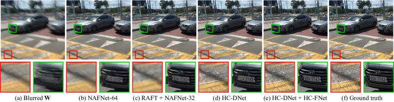
Figure 4: Deblurred results on the HC-Blur dataset.

6.1 Results on the HCBlur dataset

Methods	PSNR / SSIM	Params. (M)
MIMO-UNet+ [11]	22.42 / 0.5966	16.11
Uformer-B† [44]	23.31 / 0.6332	50.88
HINet [7]	23.60 / 0.6360	88.67
NAFNet-32 [8]	23.60 / 0.6363	17.11
NAFNet-64 [8]	24.18 / 0.6607	67.89
RAFT + NAFNet-32	24.39 / 0.6597	18.14
HC-DNet	26.20 / 0.7274	9.63
HC-DNet + HC-FNet	26.83 / 0.7413	11.69

Table 1: Quantitative comparison of deblurring methods on the HCBlur dataset. The $\dagger$ indicates that the method was evaluated using patch-wise testing due to the memory limitation, even with an 80GB memory GPU.

We evaluate the proposed method and other deblurring methods on the HCBlur test set. We compare single image deblurring methods, including state-of-the-art CNN methods [11, 7, 8] and a transformer-based method [44]. To show the effectiveness of ultra-wide burst images $\mathbf{UWs}$, we also compare a deblurring method based on an image of $\mathbf{UWs}$, denoted by ‘RAFT + NAFNet-32’. Specifically, we estimate an optical flow between the center frame of $\mathbf{UWs}$ and a resized version of the blurred $\mathbf{W}$, and then upsample the flow to the resolution of $\mathbf{W}$. Then, we extract the feature of the center frame using a NAFBlock and then warp the feature using the flow, following the same alignment process as HC-FNet. Then, NAFNet [8] performs deblurring by taking the features and blurred images as inputs. The optical flow network [41] used for alignment is also jointly trained during the training process.

The proposed method is compared with the other potential methods in Table 1. The proposed method achieves the best performance among the other methods. Especially, HC-DNet itself already outperforms the other competitors. The results show that the estimated blur kernel from $\mathbf{UWs}$ significantly improves the deblurring performance. The ‘HC-DNet + HC-FNet’ achieves the best performance as HC-FNet further improves the performance by fusing details of $\mathbf{UWs}$. Otherwise, all single image deblurring methods have inferior performance. ‘RAFT + NAFNet-32’ achieves much better performance than the single image deblurring methods, but the performance is inferior compared to the proposed method.

Fig. 4 shows qualitative results on the HCBlur dataset. The figure clearly demonstrates that both HC-DNet and ‘HC-DNet + HC-FNet’ produce significantly sharper images than other methods. HC-DNet produces a slightly blurry image due to large motion, but HC-FNet effectively enhances the deblurred image by exploiting information from the $\mathbf{UWs}$. We also present qualitative results on real-world blurred images. Fig. 5 shows our methods consistently produce sharper images compared to other methods. More qualitative results are provided in the supplement.

Figure 5: Deblurred results on real-world image.

6.2 Ablation Study

Methods	PSNR / SSIM
HC-DNet	22.80 / 0.6068
+ KGC [19]	24.97 / 0.6736
+ KAM [16]	24.98 / 0.6742
+ Concat	25.02 / 0.6764
+ KDB w/o CA	25.61 / 0.7065
+ KDB	25.68 / 0.7085

Table 2: Ablation study of HC-DNet.

DeblurNet	Alignment	Fusion	PSNR / SSIM
x	RAFT	TSA [43]	23.23 / 0.5984
NAFNet-32	RAFT	TSA [43]	24.06 / 0.6500
HC-DNet	Non-align	TSA [43]	26.69 / 0.7393
HC-DNet	BIPNet [13]	TSA [43]	26.73 / 0.7394
HC-DNet	RAFT	Avg	26.74 / 0.7414
HC-DNet	RAFT	Trans Att [27]	26.78 / 0.7404
HC-DNet	RAFT	TSA [43]	26.83 / 0.7413

Table 3: Ablation study of HC-FNet.

In this section, we will show the impact of various components within HC-DNet and HC-FNet, which are trained over 300,000 and 150,000 iterations with a batch size of 8, respectively. An additional ablation study, e.g., on the effect of the number of burst shot images, can be found in the supplementary material.

Ablation study of HC-DNet Table 2 shows the deblurring performance of different methods for utilizing blur kernels. We compare the proposed method, kernel deformable block (KDB), with methods that do not use a blur kernel, as well as those employing simple concatenation, kernel guide convolution (KGC) [19], and kernel attention module (KAM) [16]. The KGC utilizes the blur kernel to linearly transform features in the deblurring network, while the KAM employs the blur kernel to determine weights for pixel-wise channel attention. Additionally, we evaluate a variation of kernel deformable block, which does not incorporate channel attention. The table shows that the blur kernel significantly improves the deblurring performance even with simple concatenating, but the proposed KDB achieves more significant performance. Also, channel attention further improves performance, while KGC and KAM perform poorly, even worse than simple concatenation.

Ablation study of HC-FNet. Table 3 shows the effects of different components of HC-FNet. To demonstrate the importance of the deblurring module, we compare HC-FNet without using the deblurring network and using a single-image deblurring network (i.e., NAFNet [8]). The performance of both methods is inferior compared to the proposed method. The results show that the requirement of a deblurring module and single image deblurring is insufficient for hybrid camera deblurring. We compare our method with the alignment method used in BIPNet [13], which implicitly aligns features using deformable convolution. As shown in the table, the alignment method of BIPNet [13] has an inferior performance compared to the optical flow-based alignment. We also compare temporal and spatial attention (TSA) [43] with the transposed attention [27]. The table shows TSA achieves better performance than the transposed attention.

7 Conclusion

We have introduced the first learning-based hybrid camera deblurring method. We propose a novel method that includes HC-DNet and HC-FNet, which utilize low-resolution burst images as a blur kernel and an input of burst imaging, respectively. Additionally, we have presented the HC-Blur dataset for training and evaluating deblurring methods. Our experiments have demonstrated the effectiveness of the proposed methods on the HC-Blur dataset and real-world blurred images.

— Supplementary Material —

In this supplement, we present visualizations of the intermediate results of the proposed method, details of synthesizing the HCBlur dataset, and an additional experimental result omitted from the main paper due to the space limit. Additionally, we provide additional qualitative results on the HCBlur dataset and real-world images.

Appendix A Visualization of Blur Kernel

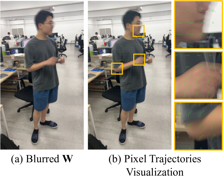
Figure 6: Visualization of pixel-wise blur kernels.

We provide an example of the per-pixel blur kernels estimated from ultra-wide burst images $\mathbf{UWs}$ in the Fig. 6. We visualize the blur kernels by linearly interpolating the values between time stamps. As shown in the figure, the estimated blur kernels are well-matched to the motion of the blurred wide-angle image, even with the dynamic object.

Appendix B Visualization of FOV Alignment

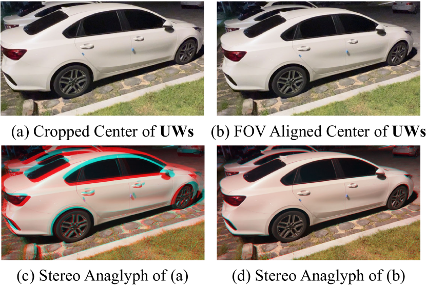
Figure 7: Example images of the simple cropping and the FOV alignment. We present stereo-anaglyph images, where the aligned center frame of $\mathbf{UWs}$ and a ground truth image are overlaid by red and cyan channels, respectively.

Fig. 7 shows example images of naïve cropping, as adopted by  [23, 42, 24], and our proposed FOV alignment technique. We also provide stereo-anaglyph images corresponding to each method, where the aligned image and a ground truth image are overlaid by red and cyan channels, respectively. As shown in the Fig. 7(c), the result of the cropping is largely misaligned with the ground truth, resulting in the presence of edges of red and cyan colors. Otherwise, the results of FOV alignment are well-aligned compared to the cropping. Note that, the FOV alignment cannot ensure the per-pixel alignment accuracy, as the method assumes a planar depth. However, it is more accurate than the previous approach of naïve cropping and provides sufficient alignment for reliable blur kernels estimation.

Appendix C Visualization of Per-pixel Alignment of UWs

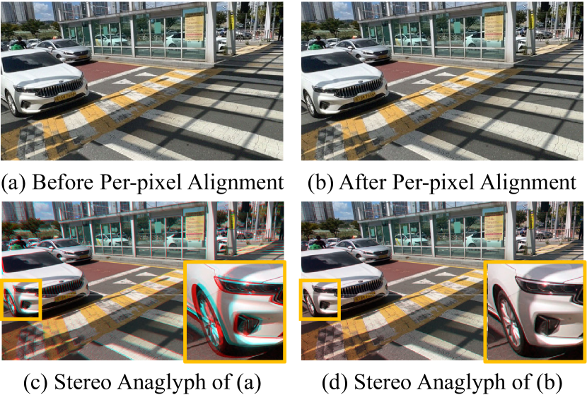
Figure 8: Example images of before and after the per-pixel alignment. We present stereo-anaglyph images, where the aligned center frame of $\mathbf{UWs}$ and a ground truth image are overlaid by red and cyan channels, respectively.

The proposed HC-FNet takes ultra-wide burst images $\mathbf{UWs}$ to produce the final enhanced output. Accurate alignment among burst images is essential to the burst imaging techniques [3, 13, 27]. To achieve accurate alignment, we perform an additional per-pixel alignment step on ultra-wide burst images $\mathbf{UWs}$ using the deblurred image $\mathbf{W}$ from HC-DNet. Fig. 8 shows result images before and after the per-pixel alignment step, along with their corresponding stereo-anaglyph images. The figure shows that the per-pixel alignment step effectively corrects the remaining misalignment.

Appendix D Details of Realistic Blur Synthesis Pipeline

Rim et al. [32] introduced a realistic blur synthesis pipeline to improve the generalization ability of a synthetic dataset on real-world blurred images. This is important because a deblurring network trained on a naïve synthetic dataset usually fails to deblur real-world blurred images. Following [32], we applied a realistic blur synthesis pipeline on the HCBlur dataset, including frame interpolation, saturation synthesis, and noise synthesis.

To reduce the discontinuity of blur, we applied a frame interpolation method [49] before averaging frames of wide-angle videos. We increased the frames per second of wide-angle videos from 30 to 480 fps by applying the frame interpolation method to the videos.

We also adopted saturation synthesis to generate realistic light streaks. For the saturation synthesis, we used the mask-based saturation synthesis [32] as:

$$I^{w}_{sat}=\textrm{clip}(I^{w}_{syn}+\alpha M^{w}_{sat})$$ (11)

where $I^{w}_{syn}$ is a blurred wide-angle image after averaging, and $M^{w}_{sat}$ is a saturation mask computed by averaging saturated pixels. $\textrm{clip}(\cdot)$ is a clipping function and $\alpha$ is a scaling factor randomly sampled from a uniform distribution $\mathcal{U}(0.25,2.75)$.

To simulate noise realistically, we converted images to the raw-RGB space, synthesized Poisson-Gaussian noise, and converted them back to the original color space (i.e., the sRGB color space). For converting the color space, color conversion matrixes of wide-angle and ultra-wide cameras are estimated using color chart images. We calibrated noise parameters of two cameras and then randomly synthesized noise on blurred $\mathbf{W}$ and $\mathbf{UWs}$. We model noise in an image as:

$$I_{noisy}=(I+N_{shot})+N_{read}$$

where $I_{noisy}$ is a noisy image and $I$ is a clean image. $N_{shot}$ and $N_{read}$ are shot noise and read noise, respectively. We use the Poisson noise and Gaussian noise model for the shot noise and read noise as follows:

$$(I+N_{shot}) \sim \mathcal{P}\left(\frac{I_{photon}}{\lambda_{shot}}\right)\lambda_{shot}$$ (12)

$$N_{read} \sim \mathcal{N}(0,\lambda_{read})$$ (13)

where $I_{photon}$ is the number of photons in the clean image. $\lambda_{shot}$ and $\lambda_{read}$ are shot noise (i.e., a mean of Poisson distribution $\mathcal{P}$) and read noise parameters (i.e., a variance of Gaussian distribution $\mathcal{N}$), respectively. We calibrated shot and read noise parameters for each camera across a range of ISO settings, from ISO 100 to 2500. To generate noises of various ISO values, we model the linear relationships of ISO values, shot noise, and read noise parameters, similar to [4]. Specifically, we first randomly sampled ISO values of wide and ultra-wide cameras as:

$$\textrm{ISO}_{w} \sim \mathcal{U}(100,800)$$ (14)

$$\textrm{ISO}_{uw} \sim \mathcal{U}(1.0,4.0)\times\textrm{ISO}_{w}$$ (15)

where $\mathcal{U}$ is a uniform distribution. $\textrm{ISO}_{w}$ is a randomly sampled ISO value of the wide camera, $\textrm{ISO}_{uw}$ is a ISO value of the ultra-wide camera. We increased the ISO values for the ultra-wide camera to simulate that the wide camera image $\mathbf{W}$ is blurred but less noisy, while the ultra-wide images $\mathbf{UWs}$ have more noise than $\mathbf{W}$.

Then, we use a linear model between the ISO values and the shot noise parameters as follows:

$$\hat{\lambda}^{w}_{shot}=1.8768\mathrm{e}{-06}\times\textrm{ISO}_{w}+9.1875\mathrm{e}{-05}$$ (16)

$$\hat{\lambda}^{uw}_{shot}=3.6760\mathrm{e}{-06}\times\textrm{ISO}_{uw}+5.8747\mathrm{e}{-04}$$ (17)

where $\hat{\lambda}^{w}_{shot}$ and $\hat{\lambda}^{uw}_{shot}$ are shot noise parameters for ISO values of each camera. The multipliers and intercepts are estimated from the calibrated shot and read noise parameters using linear regression.

We also estimated the linear relationship between the shot and read noise parameters following [4]. We model read noise parameters for each camera as:

$$log(\hat{\lambda}^{w}_{read})=1.1137\times log(\hat{\lambda}^{w}_{shot})-5.4715$$ (18)

$$log(\hat{\lambda}^{uw}_{read})=1.0753\times log(\hat{\lambda}^{uw}_{shot})-5.0671$$ (19)

where $\lambda^{w}_{read}$ and $\lambda^{uw}_{read}$ are read noise parameters of the wide-angle and ultra-wide cameras, respectively. We randomly sampled ISO values, shot, and read noise parameters and then synthesized noise on blurred $\mathbf{W}$ and $\mathbf{UWs}$ using Eq. (12) and Eq. (13). In indoor or night scenes, the ultra-wide burst images $\mathbf{UWs}$ already contain significant noise, so we skipped noise synthesis on images of $\mathbf{UWs}$ captured with ISO values exceeding 400.

Appendix E Effects of the Number of Images

The Number of Frames	PSNR / SSIM
3	22.80 / 0.6090
5	25.00 / 0.6760
7	25.90 / 0.7063
9	26.25 / 0.7202
11	26.46 / 0.7275

Table 4: Deblurring performance according to the number of frames in $\mathbf{UWs}$.

In this section, we show how the deblurring performance of the proposed method is influenced by the number of images in $\mathbf{UWs}$. We evaluate the deblurring performance on the HCBlur dataset by varying the number of frames in $\mathbf{UWs}$. However, the HCBlur dataset includes a variable number of frames in $\mathbf{UWs}$, making it challenging to evaluate using a consistent number of frames. To this end, we subsampled 411 pairs containing over 11 frames in $\mathbf{UWs}$ from the test set of the HCBlur dataset. We then compared the deblurring performance by varying the number of frames in $\mathbf{UWs}$, ranging from 3 to 11. Table 4 shows the deblurring performance significantly improves with the number of frames on $\mathbf{UWs}$ increases. This indicates that more information from $\mathbf{UWs}$ is indeed beneficial for deblurring. In the case of three frames, the performance significantly drops because the HCBlur training set does not include three frames of $\mathbf{UWs}$.

Appendix F Additional Qualitative Results

Fig. 9 and Fig. 10 show additional deblurred results on the HCBlur dataset and real-world images, respectively. These figures demonstrate the proposed method successfully deblur compared to the other methods.

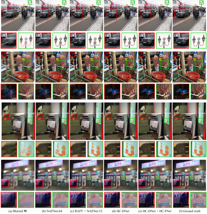
Figure 9: Deblurred results on the HCBlur dataset.

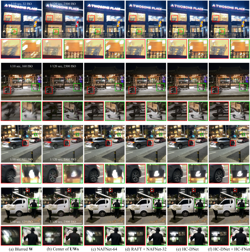
Figure 10: Deblurred results on real-world images.

References

- [1] AVCaptureMultiCamSession. https://developer.apple.com/documentation/avfoundation/avcapturemulticamsession.
- Ben-Ezra and Nayar [2003] M. Ben-Ezra and S.K. Nayar. Motion deblurring using hybrid imaging. In CVPR, 2003.
- Bhat et al. [2021] Goutam Bhat, Martin Danelljan, Luc Van Gool, and Radu Timofte. Deep burst super-resolution. In CVPR, 2021.
- Brooks et al. [2019] Tim Brooks, Ben Mildenhall, Tianfan Xue, Jiawen Chen, Dillon Sharlet, and Jonathan T Barron. Unprocessing images for learned raw denoising. In CVPR, 2019.
- Carbajal et al. [2023] Guillermo Carbajal, Patricia Vitoria, José Lezama, and Pablo Musé. Blind motion deblurring with pixel-wise kernel estimation via kernel prediction networks. IEEE Trans. Comput. Imaging, 2023.
- Chakrabarti [2016] Ayan Chakrabarti. A neural approach to blind motion deblurring. In ECCV, 2016.
- Chen et al. [2021] Liangyu Chen, Xin Lu, Jie Zhang, Xiaojie Chu, and Chengpeng Chen. Hinet: Half instance normalization network for image restoration. In CVPRW, 2021.
- Chen et al. [2022] Liangyu Chen, Xiaojie Chu, Xiangyu Zhang, and Jian Sun. Simple baselines for image restoration. In ECCV, 2022.
- Cho and Lee [2009] Sunghyun Cho and Seungyong Lee. Fast motion deblurring. ACM TOG, 2009.
- Cho and Lee [2017] Sunghyun Cho and Seungyong Lee. Convergence analysis of map based blur kernel estimation. In ICCV, 2017.
- Cho et al. [2021] Sung-Jin Cho, Seo-Won Ji, Jun-Pyo Hong, Seung-Won Jung, and Sung-Jea Ko. Rethinking coarse-to-fine approach in single image deblurring. In ICCV, 2021.
- Collins [1996] Robert T Collins. A space-sweep approach to true multi-image matching. In CVPR, 1996.
- Dudhane et al. [2022] Akshay Dudhane, Syed Waqas Zamir, Salman Khan, Fahad Shahbaz Khan, and Ming-Hsuan Yang. Burst image restoration and enhancement. In CVPR, 2022.
- Dudhane et al. [2023] Akshay Dudhane, Syed Waqas Zamir, Salman Khan, Fahad Shahbaz Khan, and Ming-Hsuan Yang. Burstormer: Burst image restoration and enhancement transformer. In CVPR, 2023.
- Evangelidis and Psarakis [2008] Georgios D Evangelidis and Emmanouil Z Psarakis. Parametric image alignment using enhanced correlation coefficient maximization. IEEE TPAMI, 2008.
- Fang et al. [2023] Zhenxuan Fang, Fangfang Wu, Weisheng Dong, Xin Li, Jinjian Wu, and Guangming Shi. Self-supervised non-uniform kernel estimation with flow-based motion prior for blind image deblurring. In CVPR, 2023.
- Fergus et al. [2006] Rob Fergus, Barun Singh, Aaron Hertzmann, Sam T. Roweis, and William T. Freeman. Removing camera shake from a single photograph. ACM TOG, 2006.
- Hu et al. [2018] Jie Hu, Li Shen, and Gang Sun. Squeeze-and-excitation networks. In CVPR, 2018.
- Kaufman and Fattal [2020] Adam Kaufman and Raanan Fattal. Deblurring using analysis-synthesis networks pair. In CVPR, 2020.
- Kingma and Ba [2014] Diederik P Kingma and Jimmy Ba. Adam: A method for stochastic optimization. arXiv preprint arXiv:1412.6980, 2014.
- Kupyn et al. [2018] Orest Kupyn, Volodymyr Budzan, Mykola Mykhailych, Dmytro Mishkin, and Jiří Matas. Deblurgan: Blind motion deblurring using conditional adversarial networks. In CVPR, 2018.
- Kupyn et al. [2019] Orest Kupyn, Tetiana Martyniuk, Junru Wu, and Zhangyang Wang. Deblurgan-v2: Deblurring (orders-of-magnitude) faster and better. In ICCV, 2019.
- Lai et al. [2022] Wei-Sheng Lai, YiChang Shih, Lun-Cheng Chu, Xiaotong Wu, Sung-Fang Tsai, Michael Krainin, Deqing Sun, and Chia-Kai Liang. Face deblurring using dual camera fusion on mobile phones. ACM TOG, 2022.
- Lee et al. [2022] Junyong Lee, Myeonghee Lee, Sunghyun Cho, and Seungyong Lee. Reference-based video super-resolution using multi-camera video triplets. In CVPR, 2022.
- Li et al. [2008] Feng Li, Jingyi Yu, and Jinxiang Chai. A hybrid camera for motion deblurring and depth map super-resolution. In CVPR, 2008.
- Lowe [2004] David G Lowe. Distinctive image features from scale-invariant keypoints. IJCV, 2004.
- Mehta et al. [2023] Nancy Mehta, Akshay Dudhane, Subrahmanyam Murala, Syed Waqas Zamir, Salman Khan, and Fahad Shahbaz Khan. Gated multi-resolution transfer network for burst restoration and enhancement. In CVPR, 2023.
- Nah et al. [2017] Seungjun Nah, Tae Hyun Kim, and Kyoung Mu Lee. Deep multi-scale convolutional neural network for dynamic scene deblurring. In CVPR, 2017.
- Nah et al. [2019] Seungjun Nah, Sungyong Baik, Seokil Hong, Gyeongsik Moon, Sanghyun Son, Radu Timofte, and Kyoung Mu Lee. Ntire 2019 challenge on video deblurring and super-resolution: Dataset and study. In CVPRW, 2019.
- Pan et al. [2016] Jinshan Pan, Deqing Sun, Hanspeter Pfister, and Ming-Hsuan Yang. Blind image deblurring using dark channel prior. In CVPR, pages 1628–1636, 2016.
- Pan et al. [2019] Liyuan Pan, Richard Hartley, Miaomiao Liu, and Yuchao Dai. Phase-only image based kernel estimation for single image blind deblurring. In CVPR, 2019.
- Rim et al. [2022] Jaesung Rim, Geonung Kim, Jungeon Kim, Junyong Lee, Seungyong Lee, and Sunghyun Cho. Realistic blur synthesis for learning image deblurring. In ECCV, 2022.
- Shan et al. [2008] Qi Shan, Jiaya Jia, and Aseem Agarwala. High-quality motion deblurring from a single image. ACM TOG, 2008.
- Shen et al. [2019] Ziyi Shen, Wenguan Wang, Jianbing Shen, Haibin Ling, Tingfa Xu, and Ling Shao. Human-aware motion deblurring. In ICCV, 2019.
- Su et al. [2017] Shuochen Su, Mauricio Delbracio, Jue Wang, Guillermo Sapiro, Wolfgang Heidrich, and Oliver Wang. Deep video deblurring for hand-held cameras. In CVPR, 2017.
- Sun et al. [2015] Jian Sun, Wenfei Cao, Zongben Xu, and Jean Ponce. Learning a convolutional neural network for non-uniform motion blur removal. In CVPR, 2015.
- Sun et al. [2013] Libin Sun, Sunghyun Cho, Jue Wang, and James Hays. Edge-based blur kernel estimation using patch priors. In ICCP, 2013.
- Tai et al. [2008] Yu-Wing Tai, Hao Du, Michael S. Brown, and Stephen Lin. Image/video deblurring using a hybrid camera. In CVPR, 2008.
- Tai et al. [2010] Yu-Wing Tai, Hao Du, Michael S. Brown, and Stephen Lin. Correction of spatially varying image and video motion blur using a hybrid camera. IEEE TPAMI, 2010.
- Tao et al. [2018] Xin Tao, Hongyun Gao, Xiaoyong Shen, Jue Wang, and Jiaya Jia. Scale-recurrent network for deep image deblurring. In CVPR, 2018.
- Teed and Deng [2020] Zachary Teed and Jia Deng. Raft: Recurrent all-pairs field transforms for optical flow. In ECCV, 2020.
- Wang et al. [2021] Tengfei Wang, Jiaxin Xie, Wenxiu Sun, Qiong Yan, and Qifeng Chen. Dual-camera super-resolution with aligned attention modules. In ICCV, 2021.
- Wang et al. [2019] Xintao Wang, Kelvin C.K. Chan, Ke Yu, Chao Dong, and Chen Change Loy. Edvr: Video restoration with enhanced deformable convolutional networks. In CVPRW, 2019.
- Wang et al. [2022] Zhendong Wang, Xiaodong Cun, Jianmin Bao, Wengang Zhou, Jianzhuang Liu, and Houqiang Li. Uformer: A general u-shaped transformer for image restoration. In CVPR, 2022.
- Xu and Jia [2010] L. Xu and J. Jia. Two-phase kernel estimation for robust motion deblurring. In ECCV, 2010.
- Xu et al. [2013] Li Xu, Shicheng Zheng, and Jiaya Jia. Unnatural L0 sparse representation for natural image deblurring. In CVPR, 2013.
- Zamir et al. [2021] Syed Waqas Zamir, Aditya Arora, Salman Khan, Munawar Hayat, Fahad Shahbaz Khan, Ming-Hsuan Yang, and Ling Shao. Multi-stage progressive image restoration. In CVPR, 2021.
- Zamir et al. [2022] Syed Waqas Zamir, Aditya Arora, Salman Khan, Munawar Hayat, Fahad Shahbaz Khan, and Ming-Hsuan Yang. Restormer: Efficient transformer for high-resolution image restoration. In CVPR, 2022.
- Zhang et al. [2023] Guozhen Zhang, Yuhan Zhu, Haonan Wang, Youxin Chen, Gangshan Wu, and Limin Wang. Extracting motion and appearance via inter-frame attention for efficient video frame interpolation. In CVPR, 2023.
- Zhang [2000] Zhengyou Zhang. A flexible new technique for camera calibration. IEEE TPAMI, 2000.
- Zhu et al. [2019] Xizhou Zhu, Han Hu, Stephen Lin, and Jifeng Dai. Deformable convnets v2: More deformable, better results. In CVPR, 2019.