ParamISP: Learned Forward and Inverse ISPs using Camera Parameters
—– Supplementary Material —–

S1 Overview

In this supplementary material, we describe two additional applications: deblurring dataset synthesis and camera-to-camera transfer (Sec. S2). We then provide details and an ablation study on the input features used in LocalNet and GlobalNet (Sec. S3), as well as training strategy (Sec. S4). Finally, we present additional quantitative and qualitative results (Sec. S5), along with the detailed architecture of ParamISP (Sec. S6).

S2 Additional Applications

ParamISP can be applied to various applications (e.g., deblurring dataset synthesis, RAW deblurring, HDR reconstruction, and camera-to-camera transfer) unlike previous methods. In this section, we describe two additional applications (i.e., deblurring dataset synthesis, camera-to-camera transfer) that were not covered in the main paper. We find that joint fine-tuning on separately trained forward and inverse ISP networks brings additional performance improvements in applications. Therefore, before applying ParamISP to applications excluding camera-to-camera transfer, we conduct additional joint fine-tuning.

In the joint fine-tuning stage, we train our pretrained forward and inverse ISP networks for 450 epochs with an initial learning rate of $1.0\times 10^{-4}$. We jointly fine-tune separately trained forward and inverse ISP networks in an end-to-end manner using loss $\mathcal{L}_{joint}$:

$$\mathcal{L}_{joint} =\|f_{for}(f_{inv}(I_{sRGB}))-I_{sRGB}\|_{1}$$ (S1)

$$\,\,\,\,\,\,\,\,\,\,+\|f_{inv}(I_{sRGB})-I_{RAW}\|_{1},$$

where $f_{for}$ and $f_{inv}$ are the forward and inverse ISP networks, respectively, and $I_{sRGB}$ is an sRGB image. Other training conditions are the same as those explained in Sec. 4 of the main paper.

S2.1 Deblurring Dataset Synthesis

Method	Synthetic				Real
	CycleISP  [14]	InvISP  [13]	RSBlur  [10]	ParamISP (Ours)	RealBlur-J  [9]
PSNR$\uparrow$	29.98	31.06	31.16	31.31	31.82
SSIM$\uparrow$	0.8806	0.9134	0.9142	0.9148	0.9203

Table S1: Quantitative results of deblurring dataset synthesis. Our dataset synthesis outperforms all the other synthesis methods. While ours still achieves lower performance than the RealBlur-J training set, this is partly due to the photometric misalignment present in the RealBlur-J dataset.

It is essential to reflect the camera ISP in order to synthesize a realistic image restoration dataset such as deblurring datasets [10]. ParamISP can enhance the accuracy of synthetic deblurring datasets as it can more accurately model real-world camera ISPs. Tab. S1 shows a comparison among different dataset synthesis approaches. On the table, RSBlur [10] is a baseline model that uses a simple parametric ISP model, while InvISP [13], CycleISP [14], and ParamISP mean variants of the RSBlur pipeline whose ISP model is replaced by the corresponding ISP models. For fair comparisons, we train the other ISP models according to their respective learning approaches. We synthesize deblurring datasets using each of the approaches on the table, train a deblurring model [3] using each dataset, and evaluate their performance on the RealBlur-J test set [9], which is a real-world blur dataset. The last column of the table represents the results obtained by directly training the deblurring model on the RealBlur-J train set, and we consider this as the upper bound.

As Tab. S1 shows, ParamISP achieves the closest PSNR to the upper bound, outperforming all the other synthesis approaches. Interestingly, InvISP [13] and CycleISP [14] achieve worse performance than RSBlur [10] although they are learnable approaches. This is because they primarily focus on cyclic reconstruction (sRGB-to-RAW-to-sRGB) and are less suitable for applications that manipulate RAW images as described in the main paper. Specifically, CycleISP uses the input sRGB image for restoring the tone when reconstructing an sRGB image back from a RAW image. Here, for the smooth tone restoration of CycleISP, we apply the same blur kernel used to create the blurry RAW image to the input sharp sRGB image, rather than using the input sharp sRGB image directly. InvISP uses a single normalizing flow-based invertible network, resulting in near-perfect reconstruction quality for cyclic reconstruction. However, its quality significantly degrades when the intermediate RAW images are altered.

While our method outperforms all the other synthetic dataset generation processes both in PSNR and SSIM, it still achieves lower performance than the upper bound model trained using the RealBlur-J training set. We emphasize that the performance gap between the upper bound and ours is partly due to the existence of remaining photometric misalignment in the blurry and sharp image pairs in the RealBlur-J dataset. The sharp and blurry images of the RealBlur-J dataset were captured by different cameras, so they have slightly different tones. While the postprocessing process of the RealBlur-J dataset applies photometric alignment to mitigate this issue, the images in the dataset still have remaining tone difference, which could only be learned from the RealBlur-J training set. Dataset synthesis methods that synthesize blurry images using only sharp images are unable to depict such tone difference between different cameras and, in fact, there is no need to depict such tone differences for the purpose of deblurring. Fig. S1 shows a qualitative comparison. The deblurring model trained with ParamISP visually outperforms each deblurring model trained with other methods, including the upper bound RealBlur-J.

S2.2 Camera-to-Camera Transfer

Given an sRGB image, ParamISP can manipulate the image as if it was taken by a different camera using the inverse and forward ISP networks trained on the different camera. Fig. S2 qualitatively shows the camera-to-camera transfer results of ParamISP. The resulting camera-transferred images (2nd and 4th images) show color tone changes from the input images (1st and 3rd images) without any noticeable artifacts.

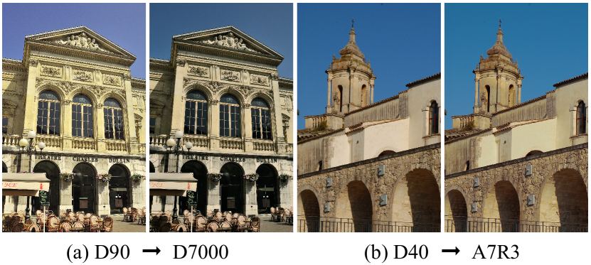
Figure S2: Qualitative results of camera-to-camera transfer.

S3 Input Features for LocalNet and GlobalNet

It is reported that leveraging the gradient map and color histogram maps improves the ISP network performance by several previous works [7, 6, 8]. In our preliminary experiments, we also find a similar finding. Based on this, we design our LocalNet and GlobalNet to be fed additional input features as well as an input image. As additional input features, we include a gradient map, a soft histogram map, and an over-exposure mask to improve the ISP network performance. For the gradient map, we apply the Sobel filter [5] on an input image and compute per-channel gradient maps in vertical and horizontal directions, resulting in a 6-channel gradient map. For the soft histogram map, we compute the soft histogram [8], for which we measure the relative distance between each channel value of a pixel and the center of histogram bins. In practice, we use 28 histogram bins, resulting in an 84-channel soft histogram map. We also include an over-exposure mask as a hint for restoring pixels of range-clipped values, where we compute the mask by setting its values as $10\max(x-\tau,0)$ where $x$ is a pixel value of an input image, and $\tau$ is a threshold. We use 0.9 as the threshold in our implementation.

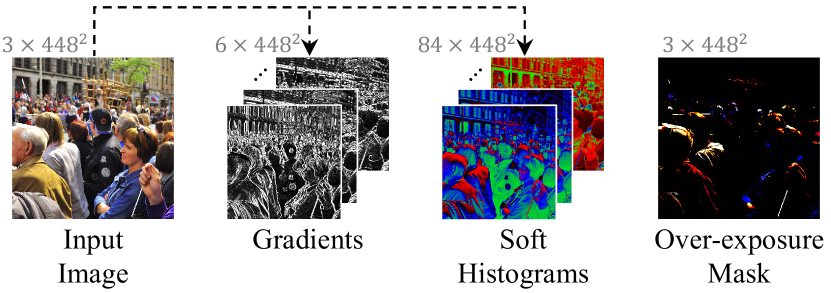
Figure S3: Input features of LocalNet and GlobalNet.

Ablation Study To validate the effects of the input features, we conduct an ablation study on RAW reconstruction using the D7000 images of the RAISE dataset [4]. Tab. S2 shows a quantitative ablation study on the input features of LocalNet and GlobalNet. To analyze only the effects of the input features, we use our model without ParamNet as the baseline (4th column). We prepare our baseline with its three model variants, where LocalNet and GlobalNet in each model variant do not use each one of the three input features.

It may be unnecessary to explicitly provide hand-crafted features such as image gradients and soft histograms, as a network can learn to extract such features from an input image. However, without these features, the network may not fully exploit its capacity to learn features more useful for local and global non-linear operations, resulting in low reconstruction quality (1st and 2nd columns). Furthermore, discarding an over-exposure mask may waste the network capacity in estimating and restoring pixels of range-clipped values, resulting in decreased reconstruction performance (3rd column). Additionally, in the first and second rows of Tab. S6, we describe the results of experiments conducted with various cameras and forward ISP networks to assess the impact of input features.

Input Features	w/o $A$	w/o $B$	w/o $C$	Full
PSNR$\uparrow$	34.32	34.40	34.29	34.77
SSIM$\uparrow$	0.9693	0.9665	0.9677	0.9712

Table S2: Ablation study on the impact of each input feature. $A$, $B$, and $C$ represent gradient map, soft histogram, and over-exposure mask, respectively. The results are measured on images of D7000 [4].

S4 Training Strategy

Datasets we use three datasets consisting of RAW and sRGB image pairs captured from multiple cameras: the RAISE dataset [4] from Nikon D7000, D90, and D40, the RealBlur dataset [9] from Sony A7R3; and the S7 ISP dataset [11] from Samsung Galaxy S7. The statistics of each dataset are shown in Tab. S3. We extract camera parameters from the EXIF metadata [12] included in JPEG images.

Pre-training with Images from Diverse Cameras To achieve high-quality reconstruction, we pre-train our models using datasets of multiple cameras as if they were captured by a single camera model. We then fine-tune the models for our target camera. Despite the differences across different camera models, we find that this two-stage training substantially improves the ISP performance as the ISP models can learn common knowledge on the ISP operations.

To validate our two-stage training approach, we present a quantitative ablation study result in Tab. S6. In the table, ‘Generic’, ‘Individual’, and ‘Generic$+$individual’ mean models trained using multiple camera datasets, models trained using only target camera datasets, and models trained using our two-stage training scheme, respectively. All the ‘Generic’, ‘Individual’ and ‘Generic$+$individual’ models are without ParamNet. We also include our final model ‘ParamISP’ trained using our two-stage training scheme in the table.

In the table, the ‘Individual’ models show higher RAW and sRGB reconstruction performance than the ‘Generic’ models on average as the ‘Generic’ models cannot properly learn the behaviors of specific camera models. The table also shows that the ‘Generic$+$individual’ models achieve higher performance than both ‘Generic’ and ‘individual’ models as they can exploit common knowledge on the camera ISP operations across various camera models, and at the same time, they can accurately learn the behaviors of specific camera models. Finally, our full models (ParamISP) outperform all the other models thanks to ParamNet.

Camera model	A7R3[9]	D7000[4]	D90[4]	D40[4]	S7[11]
Training #	7766	4600	1700	26	50
Validation #	200	200	100	-	20
Testing #	1000	1000	400	50	150

Table S3: Statistics of our dataset used for ParamISP.

Figure S4: Example of sRGB reconstruction with modified optical parameters (exposure time and sensitivity). The top row, from left to right, shows the target sRGB image reconstructed with the original optical parameters (a), sRGB image reconstructed with modified exposure time (b), and sRGB image reconstructed with modified sensor sensitivity (c) (the modified values are indicated in blue). In the second row, we include difference maps between the target sRGB image and the others. We visualize the color histogram of each image in the bottom row. (b) and (c) show clear difference in both difference map and histogram from the target.

S5 Additional Results

We provide additional detailed quantitative results to supplement the experimental results in the main paper: an ablation study on the effects of input features and the proposed ParamNet (Tab. S6), the training strategy (Tab. S6), and comparison on RAW & sRGB reconstruction (Tab. S6). The first two results supplement the experimental results in Sec. 4.1 of the main paper, while the last result supplements Sec. 4.2.

To supplement the experimental results in the main paper, we also include additional qualitative results. In Sec. 4.1 of the main paper, we analyze the impact of optical parameters and show quantitative ablation results in Tab. 2. Fig. S4 provides qualitative results as a supplement to this analysis. The figure shows that the proposed ParamISP can indeed effectively change its behavior for different camera parameters, mimicking the behaviors of real-world camera ISPs. Furthermore, we also show additional qualitative results on sRGB-to-RAW reconstruction (Fig. S5) and RAW-to-sRGB reconstruction (Fig. S6). In both qualitative results, ParamISP shows significantly lower errors compared to other methods, confirming its superior performance.

S6 Network Architecture

We visualize detailed network architectures for LocalNet (Fig. S7), GlobalNet (Fig. S8), and ParamNet (Fig. S9).

	Components	D7000 [4]		D90 [4]		D40 [4]		S7 [11]		A7R3 [9]		Average
		PSNR	SSIM	PSNR	SSIM	PSNR	SSIM	PSNR	SSIM	PSNR	SSIM	PSNR	SSIM
sRGB → RAW	Ours (w/o Input Features & ParamNet)	33.66	0.9646	34.50	0.9551	44.87	0.9879	34.51	0.9074	44.66	0.9892	38.44	0.9608
	$+$Input Features	34.77	0.9712	34.98	0.9672	44.95	0.9847	34.45	0.9063	46.72	0.9912	39.17	0.9641
	$+$ParamNet w/o dropout	35.64	0.9702	36.26	0.9724	45.41	0.9858	34.81	0.9007	47.47	0.9922	39.92	0.9643
	$+$w/ dropout	36.21	0.9724	36.31	0.9731	45.73	0.9883	35.14	0.9115	47.80	0.9922	40.24	0.9675
RAW → sRGB	Ours (w/o Input Features & ParamNet)	29.12	0.9399	29.46	0.9544	38.81	0.9843	28.48	0.7593	44.46	0.9806	34.07	0.9237
	$+$Input Features	29.21	0.9381	29.49	0.9558	39.08	0.9840	28.42	0.7635	44.39	0.9805	34.12	0.9244
	$+$ParamNet w/o dropout	29.87	0.9421	30.39	0.9639	39.11	0.9836	28.43	0.7668	44.63	0.9808	34.49	0.9274
	$+$w/ dropout	29.89	0.9422	30.50	0.9664	39.63	0.9849	28.60	0.7690	44.78	0.9815	34.68	0.9288

Table S4: Ablation study on the effects of input features and the proposed ParamNet. Each result was trained and evaluated using a specific camera only.

	Strategy	D7000 [4]		D90 [4]		D40 [4]		S7 [11]		A7R3 [9]		Average
		PSNR	SSIM	PSNR	SSIM	PSNR	SSIM	PSNR	SSIM	PSNR	SSIM	PSNR	SSIM
sRGB → RAW	Generic	34.62	0.9689	35.61	0.9738	41.37	0.9796	34.65	0.9082	44.04	0.9871	38.06	0.9635
	Individual	34.77	0.9712	34.98	0.9672	44.95	0.9847	34.45	0.9063	46.72	0.9912	39.17	0.9641
	Generic$+$individual	36.47	0.9758	36.59	0.9796	45.75	0.9879	34.99	0.9118	47.18	0.9920	40.20	0.9694
	ParamISP (Gen + Ind)	38.49	0.9809	37.06	0.9810	45.97	0.9877	35.20	0.9125	48.33	0.9930	41.01	0.9710
RAW → sRGB	Generic	28.71	0.9262	28.44	0.9447	34.90	0.9685	28.06	0.7580	39.51	0.9603	31.92	0.9115
	Individual	29.21	0.9381	29.49	0.9558	39.08	0.9840	28.42	0.7635	44.39	0.9805	34.12	0.9244
	Generic$+$individual	31.51	0.9491	29.50	0.9535	38.97	0.9831	28.42	0.7716	44.95	0.9823	34.67	0.9279
	ParamISP (Gen + Ind)	34.14	0.9628	30.83	0.9670	39.54	0.9844	29.02	0.7868	45.51	0.9841	35.81	0.9370

Table S5: Ablation study on the effects of the training strategy. ‘Generic’, ‘Individual’, and ‘Generic$+$individual’ mean models trained using multiple camera datasets, models trained using only target camera datasets, and models trained using our two-stage training scheme, respectively. All the ‘Generic’, ‘Individual’ and ‘Generic$+$individual’ models are without ParamNet. We also include our final model ‘ParamISP’ trained using our two-stage training scheme in the table.

	Method	D7000 [4]		D90 [4]		D40 [4]		S7 [11]		A7R3 [9]		Average
		PSNR	SSIM	PSNR	SSIM	PSNR	SSIM	PSNR	SSIM	PSNR	SSIM	PSNR	SSIM
sRGB → RAW	UPI [2]	20.67	0.7854	26.57	0.8623	22.05	0.7679	29.98	0.8482	30.48	0.9368	25.95	0.8401
	CIE XYZ Net [1]	30.04	0.9461	32.62	0.9521	38.57	0.9809	33.24	0.8918	36.42	0.9779	34.18	0.9498
	CycleISP [14]	35.52	0.9740	35.85	0.9786	42.83	0.9831	34.55	0.9056	45.35	0.9916	38.82	0.9666
	InvISP [13]	33.48	0.9685	35.39	0.9747	45.08	0.9866	34.29	0.9095	47.14	0.9924	39.08	0.9663
	ParamISP (Ours)	38.49	0.9809	37.06	0.9810	45.97	0.9877	35.20	0.9125	48.33	0.9930	41.01	0.9710
RAW → sRGB	UPI [2]	18.81	0.6326	20.30	0.8010	16.01	0.7649	20.05	0.4205	19.37	0.5324	18.91	0.6303
	CIE XYZ Net [1]	26.76	0.8703	27.61	0.9183	34.84	0.9635	27.63	0.6978	37.19	0.9396	30.81	0.8779
	InvISP [13]	30.20	0.9393	28.89	0.9448	37.86	0.9816	28.96	0.7862	43.93	0.9786	33.97	0.9261
	ParamISP (Ours)	34.14	0.9628	30.83	0.9670	39.54	0.9844	29.02	0.7868	45.51	0.9841	35.81	0.9370

Table S6: Quantitative comparison on RAW & sRGB reconstruction. Note that CycleISP is not included in this comparison because it needs an input sRGB image for sRGB reconstruction.

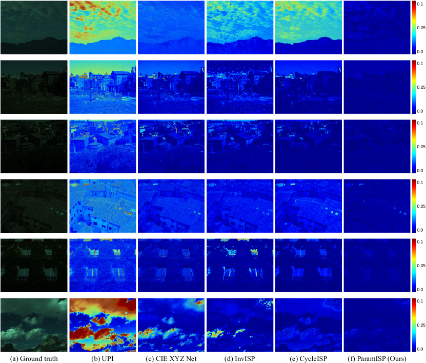
Figure S5: sRGB-to-RAW reconstruction. We show error maps between reconstructed and GT RAW images.

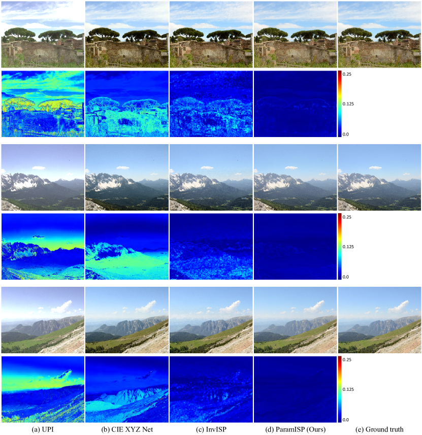
Figure S6: RAW-to-sRGB reconstruction. We show error maps between reconstructed and GT sRGB images.

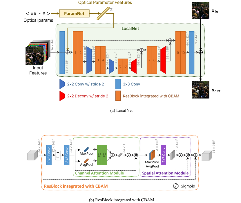
Figure S7: Detailed architecture of LocalNet.

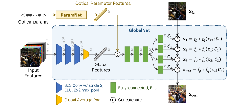
Figure S8: Detailed architecture of GlobalNet.

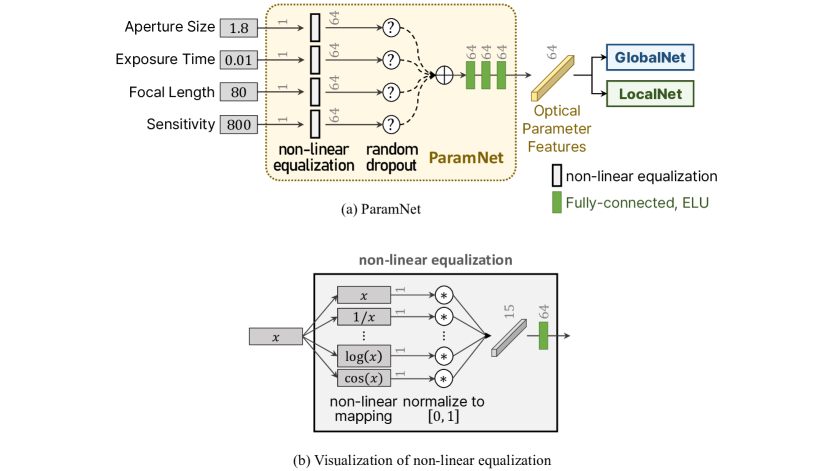
Figure S9: Detailed architecture of ParamNet.

References

- Afifi et al. [2021] M. Afifi, A. Abdelhamed, A. Abuolaim, A. Punnappurath, and M. S. Brown. Cie xyz net: Unprocessing images for low-level computer vision tasks. IEEE Transactions on Pattern Analysis and Machine Intelligence (TPAMI), 44(9):4688–4700, 2021.
- Brooks et al. [2019] T. Brooks, B. Mildenhall, T. Xue, J. Chen, D. Sharlet, and J. T. Barron. Unprocessing images for learned raw denoising. In Proceedings of the IEEE Conference on Computer Vision and Pattern Recognition (CVPR), 2019.
- Chen et al. [2022] Liangyu Chen, Xiaojie Chu, Xiangyu Zhang, and Jian Sun. Simple baselines for image restoration. In Proceedings of the European conference on computer vision (ECCV), 2022.
- Dang-Nguyen et al. [2015] D.-T. Dang-Nguyen, C. Pasquini, V. Conotter, and G. Boato. Raise: A raw images dataset for digital image forensics. In Proceedings of the 6th ACM multimedia systems conference (MMSys), 2015.
- Kanopoulos et al. [1988] N. Kanopoulos, N. Vasanthavada, and Robert L. Baker. Design of an image edge detection filter using the sobel operator. IEEE Journal of Solid-State Circuits (JSSC), 23(2):358–367, 1988.
- Lin and Zhang [2005] S. Lin and L. Zhang. Determining the radiometric response function from a single grayscale image. In Proceedings of the IEEE Conference on Computer Vision and Pattern Recognition (CVPR), 2005.
- Lin et al. [2004] S. Lin, J. Gu, S. Yamazaki, and H. Shum. Radiometric calibration from a single image. In Proceedings of the IEEE Conference on Computer Vision and Pattern Recognition (CVPR), 2004.
- Liu et al. [2020] Y.-L. Liu, W.-S. Lai, Y.-S. Chen, Y.-L. Kao, M.-H. Yang, Y.-Y. Chuang, and J.-B. Huang. Single-image hdr reconstruction by learning to reverse the camera pipeline. In Proceedings of the IEEE Conference on Computer Vision and Pattern Recognition (CVPR), 2020.
- Rim et al. [2020] J. Rim, H. Lee, J. Won, and S. Cho. Real-world blur dataset for learning and benchmarking deblurring algorithms. In Proceedings of the European Conference on Computer Vision (ECCV), 2020.
- Rim et al. [2022] J. Rim, G. Kim, J. Kim, J. Lee, S. Lee, and S. Cho. Realistic blur synthesis for learning image deblurring. In Proceedings of the European Conference on Computer Vision (ECCV), 2022.
- Schwartz et al. [2018] E. Schwartz, R. Giryes, and A. M. Bronstein. Deepisp: Toward learning an end-to-end image processing pipeline. IEEE Transactions on Image Processing (TIP), 28(2):912–923, 2018.
- Tachibanaya [2001] Tsurozoh Tachibanaya. Description of exif file format. http://www.fifi.org/doc/jhead/exif-e.html, 2001.
- Xing et al. [2021] Y. Xing, Z. Qian, and Q. Chen. Invertible image signal processing. In Proceedings of the IEEE Conference on Computer Vision and Pattern Recognition (CVPR), 2021.
- Zamir et al. [2020] S. W. Zamir, A. Arora, S. Khan, M. Hayat, F. S. Khan, M.-H. Yang, and L. Shao. Cycleisp: Real image restoration via improved data synthesis. In Proceedings of the IEEE Conference on Computer Vision and Pattern Recognition (CVPR), 2020.