Estimating Trotter Approximation Errors to Optimize Hamiltonian Partitioning for Lower Eigenvalue Errors

Abstract

One of the ways to encode many-body Hamiltonians on a quantum computer to obtain their eigen-energies through Quantum Phase Estimation is by means of the Trotter approximation. There were several ways proposed to assess the quality of this approximation based on estimating the norm of the difference between the exact and approximate evolution operators. Here, we would like to explore how these different error estimates are correlated with each other and whether they can be good predictors for the true Trotter approximation error in finding eigenvalues. For a set of small molecular systems we calculated the exact Trotter approximation errors of the first order Trotter formulas for the ground state electronic energies. Comparison of these errors with previously used upper bounds show almost no correlation over the systems and various Hamiltonian partitionings. On the other hand, building the Trotter approximation error estimation based on perturbation theory up to a second order in the time-step for eigenvalues provides estimates with very good correlations with the Trotter approximation errors. The developed perturbative estimates can be used for practical time-step and Hamiltonian partitioning selection protocols, which are paramount for an accurate assessment of resources needed for the estimation of energy eigenvalues under a target accuracy.

1 Introduction

Solving the electronic structure problem is one of the anticipated uses of quantum computing. As an eigenvalue problem with a Hamiltonian operator that can be expressed compactly, this problem is convenient for quantum computing because classical-quantum data transfer is usually a bottleneck.[1] Obtaining electronic wavefunctions and energies is one of the key procedures in first principles modelling of molecular physics since molecular energy scale is dominated by the electronic part. Yet, solving this problem scales exponentially with the size unless some approximations are made.

Fault-tolerant quantum computers offer potential advantages for efficient estimation of energy eigenvalues through exponential speedup with respect to classical methods, by means of the Quantum Phase Estimation (QPE) algorithm.[2] The QPE framework contains three main parts: 1) initial state preparation, 2) procedure for an evolution or a walker operator that involves the Hamiltonian encoding, and 3) the eigenvalue extraction. Here, we focus on the second part, two main approaches for the Hamiltonian encoding are representing the Hamiltonian exponential function via the Trotter approximation and embedding the Hamiltonian as a block of a larger unitary via decomposing the Hamiltonian as a Linear Combination of Unitaries (LCU).

Within the Trotter approximation, the target Hamiltonian is decomposed into easy-to-simulate (or fast-forwardable) Hamiltonian fragments:

$$\hat{H}=\sum_{m=1}^{M}\hat{H}_{m}$$ (1)

and the exact unitary evolution operator for an arbitrary simulation time $\tau$ is approximated as

$$\hat{U}(\tau)=e^{-i\tau\hat{H}}\approx\left(\prod_{m=1}^{M}e^{-i\hat{H}_{m}\tau/n}\right)^{n}=\left(\hat{U}_{T}(\tau/n)\right)^{n}$$ (2)

where $\hat{U}_{T}(\tau/n)$ is the Trotterized time-propagator. $e^{-i\hat{H}_{m}\tau/n}$ can be translated to quantum gates as there exist known unitary transformations $\hat{V}_{m}$ that render $\hat{H}_{m}$ into a diagonal form in the computational basis according to $\hat{H}_{m}=\hat{V}_{m}\hat{D}_{m}\hat{V}_{m}^{{\dagger}}$. In this work, for simplicity we consider the first-order Trotter formula. Higher order extensions are well-known, but the concomitant circuit depth increases exponentially with the order of the approximation.[3, 4, 5] This approximate representation of the exact time evolution operator introduces a deviation in the spectrum of the simulated time evolution unitary with respect to the exact one. For estimation of energy eigenvalues through QPE under a fixed target error, it is therefore crucial to rationalize the scaling of this deviation with the time scale used for discretization of the total simulation time as well as its dependence with different Hamiltonian partitioning schemes.

In spite of less favourable time scaling of the Trotter approach compared to the LCU based techniques, it has benefits of a lower ancilla qubit overhead and possibility for using commutation relation between terms of the Hamiltonian for formulating fast-forwardable fragments. Yet, one difficulty for practical use of the Trotter approximation is estimation of its error. This estimation is needed for choosing the evolution time-step and the overall error estimation. Another use of the Trotter approximation error is choosing the Hamiltonian partitioning that minimizes error and thus the number of steps required.

Recently, upper bounds were formulated for the norm of the difference between propagators,

$$||\hat{U}(\tau)-\hat{U}_{T}(\tau/n)^{n}||\leq\frac{\alpha\tau^{2}}{n},$$ (3)

$$\alpha={2}\sum_{m}\norm{[\hat{H}_{m},\sum_{m^{\prime}<m}\hat{H}_{m^{\prime}}]},~{}$$ (4)

which allowed one to estimate the effect of the Trotter approximation on the accuracy of dynamics. [6] Also, these estimates can be used to derive upper bounds for the energy error in QPE [7], $\Delta E\leq\alpha\tau/n$. In what follows, for brevity, we will refer to the time step as $t=\tau/n$. However, it is known in general that the Trotter upper bounds are relatively loose and using them could lead to underestimation of appropriate time-step [8]. Considering that with some simplifications $\alpha$ values can be evaluated and used to differentiate various Hamiltonian partitionings [9], it is interesting to examine how accurate $\alpha$-based trends are compared to those using the exact Trotter approximation error in eigenvalues.

Here, we investigate using the exact error calculation for small systems whether the Trotter approximation error upper bounds can be used to differentiate Hamiltonian partitionings. We also explore alternative estimates of the Trotter approximation error for eigenvalues based on time-independent perturbation theory. Such theory can be built by representing the Trotter propagator as

$$\hat{U}_{T}(t)=e^{-it\hat{H}_{\rm eff}(t)}$$ (5)

and performing perturbative analysis of the $\hat{H}_{\rm eff}(t)$ spectrum. Even though perturbative estimates are not upper bounds, they can be used for differentiating between various Hamiltonian partitioning schemes. As for predicting the Trotter step, one can use perturbative estimates as a first step in the iterative procedure suggested recently.[10]

2 Perturbative error estimates

Time-independent perturbation theory is built by considering Campbell-Baker-Hausdorff expansion of the first order Trotter evolution operator in Eq. (5)

$$\hat{H}_{\rm eff}(t)=\hat{H}+\sum_{k}\hat{V}_{k}t^{k},$$ (6)

where first few $\hat{V}_{k}$’s are derived in Appendix A.5 and can be writen as

$$\begin{split}\hat{V}_{1}&=-\frac{i}{2}\sum_{v=\mu+1}^{M}\sum_{\mu=1}^{M-1}[\hat{H}_{v},\hat{H}_{\mu}],\\ \hat{V}_{2}&=\hat{v}_{2}+\frac{i}{6}[\hat{H},\hat{V}_{1}],\\ \hat{v}_{2}&=-\frac{1}{3}\sum_{v^{\prime}=v}^{M}\sum_{v=\mu+1}^{M}\sum_{\mu=1}^{M-1}\left(1-\frac{\delta_{v^{\prime},v}}{2}\right)[\hat{H}_{v^{\prime}},[\hat{H}_{v},\hat{H}_{\mu}]].\end{split}$$ (7)

Note that in spite of $t$ dependence of $\hat{H}_{\rm eff}$, we do not need time-dependent perturbation theory since we are interested in eigenvalues of $\hat{H}_{\rm eff}$ as a function of $t$. Eigenvalues of $\hat{H}_{\rm eff}$ can be obtained as perturbative series starting from those of $\hat{H}$, focusing on the ground state energy $E_{0}$ the first order correction can be written as

$$E_{\text{GS}}^{(1)}=\langle\phi_{0}|\hat{V}_{2}|\phi_{0}\rangle t^{2}=\langle\phi_{0}|\hat{v}_{2}|\phi_{0}\rangle t^{2},$$

where $|\phi_{0}\rangle$ is electronic ground state, and the $\mathcal{O}(t)$ term vanishes due to the the anti-hermiticity of $\hat{V}_{1}$ and the real character of $\langle\phi_{0}|\hat{V}_{1}|\phi_{0}\rangle$. Another $\mathcal{O}(t^{2})$ contribution originates from the second order correction in $\hat{V}_{1}$

$$E_{\text{GS}}^{(2)} =t^{2}\sum_{n>0}\frac{|\langle\phi_{n}|\hat{V}_{1}|\phi_{0}\rangle|^{2}}{E_{\text{0}}-E_{n}},$$ (8)

where $\hat{H}|\phi_{n}\rangle=E_{n}|\phi_{n}\rangle$.

From these considerations, the Trotter-approximation error is $E_{0}^{(T)}\approx E_{0}+\varepsilon_{2}t^{2}$, where

$$\varepsilon_{2}=\langle\phi_{0}|\hat{v}_{2}|\phi_{0}\rangle+\sum_{n>0}\frac{|\langle\phi_{n}|\hat{V}_{1}|\phi_{0}\rangle|^{2}}{E_{\text{0}}-E_{n}}.$$ (9)

The calculation of $\varepsilon_{2}$ requires knowledge of eigenfunctions and spectrum of $\hat{H}$. Since the latter are not accessible for a general Hamiltonian we approximate $\varepsilon_{2}$ using eigenenergies $\{\tilde{E}_{n}\}$ and eigenstates $\{|\psi_{n}\rangle\}$ of the Fock operator $\hat{f}=\sum_{p,q}f_{p,q}\hat{a}_{p}^{\dagger}\hat{a}_{q}$ [11] instead. Then, we define an approximation to $\varepsilon_{2}$ given by

$$\varepsilon_{HF}=\langle\psi_{0}|\hat{v}_{2}|\psi_{0}\rangle+\sum_{n>0}\frac{|\langle\psi_{n}|\hat{V}_{1}|\psi_{0}\rangle|^{2}}{\tilde{E}_{\text{0}}-\tilde{E}_{n}}$$ (10)

where $\hat{f}|\psi_{n}\rangle=\tilde{E}_{n}|\psi_{n}\rangle$. It is expected $|\varepsilon_{2}-\varepsilon_{HF}|$ to become smaller with larger overlaps $\langle\phi_{n}|\psi_{n}\rangle$ and smaller $|\tilde{E}_{n}-E_{n}|$ at least for the ground and first excited states.

One further simplification of Eq. (10) is through a Common Energy Denominator Approximation (CEDA), that bypasses the requirement of knowing the whole eigenspectrum of the Fock operator, according to

$$\begin{split}\varepsilon^{(C)}_{HF}&=\langle\psi_{0}|\hat{v}_{2}|\psi_{0}\rangle+\frac{1}{\Delta{\tilde{E}}_{01}}\sum_{n>0}|\langle\psi_{n}|\hat{V}_{1}|\psi_{0}\rangle|^{2}\\ &=\langle\psi_{0}|\hat{V}_{2}|\psi_{0}\rangle+\frac{\langle\psi_{0}|\hat{V}^{2}_{1}|\psi_{0}\rangle-\langle\psi_{0}|\hat{V}_{1}|\psi_{0}\rangle^{2}}{\Delta{\tilde{E}}_{01}}\\ &=\bra{\psi_{0}}\hat{V}_{2}+\frac{\hat{V}^{2}_{1}}{\Delta{\tilde{E}}_{01}}\ket{\psi_{0}}\end{split}$$ (11)

where $\Delta\tilde{E}_{01}=\tilde{E}_{0}-\tilde{E}_{1}$. Since Eq. (11) encompasses two approximations, namely, the use of eigenspectrum and eigenfunctions of an approximate Hamiltonian as well as the CEDA, we also consider in Sec. 3 the impact solely due to CEDA in the estimation of $\varepsilon$’s by introducing

$$\varepsilon^{(C)}_{GS}=\bra{\phi_{0}}\hat{V}_{2}+\frac{\hat{V}^{2}_{1}}{E_{0}-E_{1}}\ket{\phi_{0}}.$$ (12)

3 Results and Discussion

Here, we assess correlations between the exact Trotter approximation errors and estimates for two approximate approaches based on $\alpha$ [Eq. (4)] and $H_{\rm eff}$ perturbative expressions [Eqs. (8)-(12)]. The Trotter approximation errors are obtained for electronic Hamiltonians of small molecules (H₂, LiH, BeH₂, H₂O, and NH₃) and various Hamiltonian partitioning schemes described in Appendix A. The exact Trotter approximation errors $|\Delta E_{T}|=|E^{(T)}_{0}-E_{0}|$ are computed through numerical diagonalization of $\hat{H}$ and $\hat{H}_{\text{eff}}$ [Eq. (5)] as described in Appendix A.4.

3.1 Exact Trotter approximation errors

Comparing the true errors with $\alpha$ upper-bound-based predictions in Fig. 1 (a) shows poor correlation for the qubit partitionings and even anti-correlation for the fermionic partitionings. Thus, it is not possible to determine the Hamiltonian partitioning performance in terms of the Trotter approximation error based on $\alpha$ values. Upper bounds based on $\alpha$’s are usually very loose, so we have considered an $\alpha$-like estimates based on

$$\alpha_{e}=||\hat{U}(t)-\hat{U}_{T}(t)||/t^{2},$$ (13)

where $t=1/||\hat{H}||$, which are tighter, but still provide anti-correlations, Fig. 1 (b). This discrepancy can be understood as a consequence of $\alpha$ and $\alpha_{e}$ being worst-case scenario metrics for the infidelities (with respect to exact unitary propagation) that ensue from the Trotter approximation rather than a measure of deviation with respect to the eigenspectrum of the target simulated Hamiltonian.

On the other hand, for small $t$, $|\Delta E_{T}|=\varepsilon t^{2}+\mathcal{O}(t^{3})$, and coefficient $\varepsilon$ should be exactly captured by $\varepsilon_{2}$ [Eq. (9)]. This is what is observed in Fig. 2. Other, more practical approximations to $\varepsilon_{2}$ also perform quite well. Even though $\varepsilon_{HF}$ in Eq. (10) is not an upper bound for $\varepsilon$, it is able to predict qubit-partition methods as the most accurate partitioning schemes for Trotterized time evolution, which is a consequence of the high degree of correlation between this quantity and $\varepsilon$ (Fig. 2).

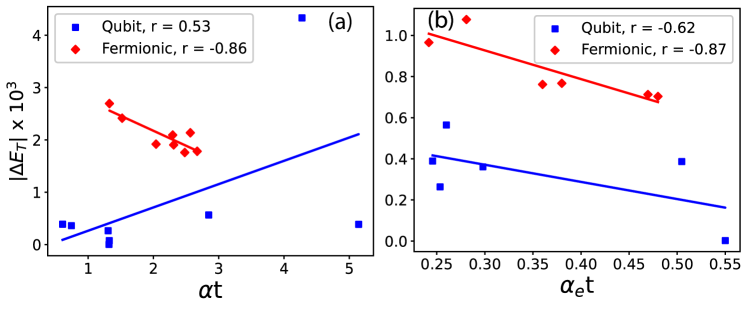
Figure 1: Correlation between $|\Delta E_{T}|=|E^{(T)}_{0}-E_{0}|$, $\alpha t$, and $\alpha_{e}t$ [Eqs. (13) and (3)]. The straight lines are obtained by a least-square fit and have correlation coefficients ($r$). Both axes for the fermionic partitioning methods are scaled by factors of 5 and 2 for panel (a) and (b), respectively, for better visualization. Appendix A.6 contains all numerical values of these plots.

Figure 2: (a) Correlation of the exact Trotter approximation error scaling $|\varepsilon|$ with the heuristic error estimate $|\varepsilon_{HF}|$. To verify the validity of perturbative estimations, we compare $|\varepsilon_{2}|$ [Eq. (9)] with $|\varepsilon|$’s. As a visual aid, the function $|\varepsilon|=|\varepsilon|$ (green) is shown, as well as the linear fittings corresponding to $\varepsilon_{HF}$ (red) and $\varepsilon_{2}$ (blue). $\varepsilon_{HF}$ features $0.99$ Pearson correlation coefficient, and $0.89$ as Spearman coefficient, whereas $\varepsilon_{2}$ is visually identical to the exact $\varepsilon$. (b) Correlations between the CEDA-approximated errors $\varepsilon^{(C)}_{GS}$ and $\varepsilon^{(C)}_{HF}$, they have 0.77 (0.88) and 0.69 (0.80) Pearson (Spearman) correlation coefficients, respectively. Numerical values are included in Appendix A.6.

One further simplification of the evaluation of perturbative estimates can be possible if there exist correlation between the contributions $\varepsilon_{V_{1}}=|\sum_{n}\frac{\langle\phi_{n}|\hat{V}_{1}|\phi_{0}\rangle}{E_{0}-E_{n}}|$ and $\varepsilon_{V_{2}}=\langle\phi_{0}|\hat{V}_{2}|\phi_{0}\rangle$. Figure 3 shows correlation for most of the systems and methods explored. This correlation allows one to build heuristic approaches for the Hamiltonian partitioning selection based on a single contribution.

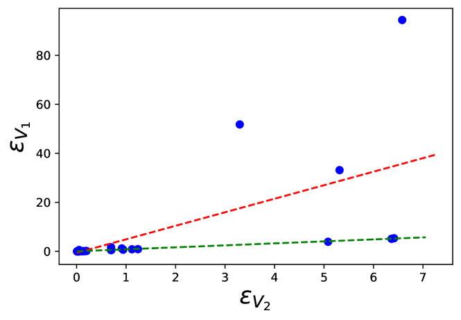
Figure 3: a) Correlation between $\varepsilon_{V_{1}}=|\sum_{n}\frac{|\langle\phi_{n}|\hat{V}_{1}|\phi_{0}\rangle|^{2}}{E_{0}-E_{n}}|$ and $\varepsilon_{V_{2}}=\langle\phi_{0}|\hat{V}_{2}|\phi_{0}\rangle$. The green-dashed line corresponds to the linear fitting of data points excluding the outliers that correspond to H₂O (GFRO and FRO), and NH₃ (FRO). A linear regression analysis of all data points (red-dashed line) yields 0.64 and 0.97 as Pearson and Spearman correlation coefficients, respectively. (b) Outlier removal yields 0.99 and 0.97 as Pearson and Spearman correlation coefficients, respectively.

Yet another simplification of the second order contribution based on CEDA is tested in Fig. 2. Results show a significant drop in the faithfulness of our accuracy-proxy when CEDA is introduced. This also holds for $\varepsilon^{(C)}_{GS}$ introduced in Eq. (12).

3.2 Resource efficiency

	$\alpha$-based			$\varepsilon$-based
Molecule	1st best ($N_{T}$)	2nd best ($N_{T}$)	3nd best ($N_{T}$)	1st best ($N_{T}$)	2nd best ($N_{T}$)	3nd best ($N_{T}$)
H2	FC SI ($4.4\times 10^{8}$)	QWC SI ($4.4\times 10^{8}$)	QWC LF ($4.4\times 10^{8}$)	FC SI ($4.91\times 10^{6}$)	QWC SI ($4.91\times 10^{6}$)	QWC LF ($4.91\times 10^{6}$)
LiH	FC SI ($2.2\times 10^{11}$)	QWC SI ($2.4\times 10^{11}$)	FC LF ($5.1\times 10^{11}$)	FC LF ($1.7\times 10^{8}$)	QWC SI ($1.9\times 10^{8}$)	FC SI ($2.13\times 10^{8}$)
BeH2	FC SI ($6.04\times 10^{11}$)	QWC SI ($7.2\times 10^{11}$)	QWC LF ($2.2\times 10^{12}$)	FC SI ($4.31\times 10^{8}$)	QWC SI ($5.02\times 10^{8}$)	QWC LF ($5.23\times 10^{8}$)
H2O	FC SI ($1.0\times 10^{13}$)	QWC SI ($1.2\times 10^{13}$)	QWC LF ($3.4\times 10^{14}$)	FC SI ($2.72\times 10^{8}$)	QWC LF ($9.08\times 10^{8}$)	QWC SI ($1.09\times 10^{9}$)
NH3	FC SI ($2.9\times 10^{13}$)	QWC SI ($3.5\times 10^{13}$)	LR LCU ($6.1\times 10^{13}$)	QWC LF ($2.9\times 10^{8}$)	FC SI ($4.7\times 10^{9}$)	QWC SI ($5.0\times 10^{9}$)

Table 1: Best resource-efficient Hamiltonian decomposition methods for eigenvalue estimation within a $10^{-3}$ h target error with a Trotterized QPE algorithm. T-gate count $N_{T}$ is given in parenthesis.

	$\varepsilon_{HF}$-based
Molecule	1st best ($N_{T}$)	2nd best ($N_{T}$)	3nd best ($N_{T}$)
H2	QWC LF($6.4\times 10^{6}$)	FC LF ($6.4\times 10^{6}$)	QWC LF ($7.4\times 10^{6}$)
LiH	QWC SI ($2.67\times 10^{8}$)	FC SI ($2.70\times 10^{8}$)	QWC LF ($3.55\times 10^{8}$)
BeH2	FC LF ($4.72\times 10^{8}$)	QWC LF ($5.62\times 10^{8}$)	FC SI ($5.8\times 10^{8}$)
H2O	FC SI ($9.78\times 10^{8}$)	QWC LF ($1.4\times 10^{9}$)	QWC SI ($1.4\times 10^{9}$)
NH3	QWC SI ($3.78\times 10^{9}$)	FC SI ($5.58\times 10^{9}$)	QWC LF ($5.77\times 10^{9}$)

Table 2: Best resource-efficient Hamiltonian decomposition methods for eigenvalue estimation within a $10^{-3}$ h target error with a Trotterized QPE algorithm. T-gate count $N_{T}$ is given in parenthesis.

Table 1 summarizes upper bound estimations of the T-gate count required for QPE under a target accuracy based on the exact scaling of Trotter approximation errors $\varepsilon$, alongside cruder estimations based on the $\alpha$ upper bounds. We notice that even though upper bound estimations on T-gate count based on the $\alpha$ Trotter approximation error bounds predict best performance of qubit decompositions, they tend to overrate the FC methods, and for NH₃, some fermionic ones. For NH₃, the best performing Hamiltonian decomposition is QWC LF, in stark contrast with previously built intuition that greedy-algorithms favour small Trotter approximation errors. For $\varepsilon$ analysis based on perturbation theory expressions we cannot establish the same trends as those found for $\alpha$’s in Ref. [9]. Finally, in Table 2 we explore the faithfulness of $\varepsilon_{HF}$ in the discrimination of the best resource-efficient methods. The $\varepsilon_{HF}$-based estimator predictions of the T-gate numbers are in the same order as those obtained based on $\varepsilon$. Also, the $\varepsilon_{HF}$-based estimator correctly suggests qubit partition methods as the most accurate compared to their fermionic counterparts. Due to similarity of T-gate numbers for various qubit partitionings, the ranking based on $\varepsilon_{HF}$ and $\varepsilon$ are different, in spite of the high degree of $\varepsilon_{HF}-\varepsilon$ correlation (Fig.2). Thus, in these cases of weakly correlated systems $\varepsilon_{HF}$ can be a good substitute for $\varepsilon$ since all the best Hamiltonian partitioning methods have very similar resource estimations and their particular order is of little importance.

4 Conclusions

We have calculated exact errors associated with the first order Trotter approximation for small molecules and different Hamiltonian partitionings. Correlations between the exact errors and previously derived $\alpha$ upper bounds were shown to be low and even negative in some cases. This confirmed loose character of the $\alpha$ based upper bounds for energies, which makes these upper bounds inadequate in determining the best Hamiltonian partitioning for a particular system. The alternative estimates of the Trotter approximation error based on perturbative analysis of effective Hamiltonian eigen-spectrum performed much better. It was shown that even though these estimates are not upper bounds they can be used to distinguish Hamiltonian partitioning more accurately in terms of the Trotter approximation error. For example, they correctly pointed out that qubit-based partitioning methods outperform the fermionic partitioning methods with the difference becoming more prominent for larger molecules.

Perturbative expression for the Trotter approximation error were further simplified to make their calculation practical. Substituting the exact eigenvalues and eigenstates to their Hartree-Fock counterparts gave accurate approximations. It can be attributed to the fact that all our systems have the weight of the HF Slater determinant higher than 97% in their ground state wavefunction. Yet, for more correlated systems one can find approximations using more accurate ansatzes. Another approximation that has been explored is CEDA. This approximation resulted in further reductions in correlations with the true errors, but it still stayed above 0.8 in Spearman correlation coefficient.

These estimations of the Trotter approximation error approximation raise two questions for future research: 1) how to optimize efficiently the Hamiltonian partitioning and ordering of its fragments based on the obtained error estimates; and 2) how to obtain upper bounds for the error estimates based on the eigen-spectrum analysis of $H_{\rm eff}$. Answering the second question will allow one to set an optimal Trotter time step for resource efficient simulation under a target energy eigenvalue estimation accuracy.

Appendix A Fermionic and Qubit-based Hamiltonian Decomposition methods

Here, we discuss the methods we used to decompose electronic Hamiltonians into fast-forwardable fragments using fermionic- and qubit-based methods. The second quantized representation of the molecular electronic Hamiltonian with $N$ single particle spin-orbitals under this representation is

$$\hat{H}=\sum_{pq=1}^{N}h_{pq}\hat{a}_{p}^{{\dagger}}\hat{a}_{q}+\sum_{pqrs=1}^{N}g_{pqrs}\hat{a}_{p}^{{\dagger}}\hat{a}_{q}\hat{a}_{r}^{{\dagger}}\hat{a}_{s}$$ (14)

where $a_{p}^{{\dagger}}$ $(a_{q})$ is the creation (annihilation) fermionic operator for the $p^{th}$ spin-orbital, $h_{pq}$ and $g_{pqrs}$ are one- and two-electron integrals.[11]

A.1 Fermionic partitioning methods

These partitioning methods are built upon the solvability of one-electron Hamiltonians using orbital rotations, according to

$$\hat{H}_{1e}=\sum_{pq}h_{pq}\hat{a}_{p}^{{\dagger}}\hat{a}_{q}=\hat{U}_{1}^{{\dagger}}\left(\sum_{p}\tilde{h}_{p}\hat{n}_{p}\right)\hat{U}_{1},$$ (15)

$$\hat{U}_{1}=\prod_{p>q}e^{\theta_{pq}(\hat{a}_{p}^{{\dagger}}\hat{a}_{q}-\hat{a}_{q}^{{\dagger}}\hat{a}_{p})}$$ (16)

where $\hat{n}_{p}=\hat{a}_{p}^{{\dagger}}\hat{a}_{q}$ occupation number operators, $\tilde{h}_{p}$ are real constants, and $\hat{U}_{1}$ is an orbital rotation parameterized by the amplitudes $\theta_{pq}$. Orbital rotations can also be employed to solve two-electron Hamiltonians that are squares of one-electron Hamiltonians as follows:

$$\hat{H}^{(LR)} =\left(\sum_{pq}h_{pq}\hat{a}_{p}^{\dagger}\hat{a}_{q}\right)^{2}=\hat{U}^{\dagger}\left(\sum_{p}\tilde{h}_{p}\hat{n}_{p}\right)^{2}\hat{U}$$ (17)

$$=\hat{U}^{\dagger}\left(\sum_{pq}\tilde{h}_{p}\tilde{h}_{q}\hat{n}_{p}\hat{n}_{q}\right)\hat{U}.$$ (18)

The matrix with entries $\lambda_{pq}=\tilde{h}_{p}\tilde{h}_{q}$ is a rank-deficient one. The form of two-electron solvable Hamiltonians by means of orbital rotations in (17) can be straightforwardly generalized by lifting the rank-deficient character of $\lambda$ matrix and regarding it as a full-rank hermitian matrix:

$$\hat{H}^{(FR)}=\hat{U}^{\dagger}\left(\sum_{pq}\lambda_{pq}\hat{n}_{p}\hat{n}_{q}\right)\hat{U}.$$ (19)

The fermionic methods that follow are classified according to whether the Hamiltonian decomposition yields fast-forwardable fragments with low- or full-rank character.

Full-rank (FR) optimization and its greedy variant: These approaches use orbital rotations to diagonalize the one-electron part and approximate the two-body interaction terms featured in Eq. (14) as a sum of full-rank Hamiltonian fragments of the form (19) [12]

$$\hat{H}=\hat{H}_{1e}+\sum_{m=2}^{M}\hat{H}_{m}^{(FR)},$$ (20)

In a FR optimization, to find the {$\hat{H}_{m}^{(FR)}$} set we introduce the G tensor according to

$$\sum_{pqrs=1}^{N}G_{pqrs}\hat{a}_{p}^{{\dagger}}\hat{a}_{q}\hat{a}_{r}^{{\dagger}}\hat{a}_{s} =\sum_{pqrs}^{N}g_{pqrs}\hat{a}_{p}^{{\dagger}}\hat{a}_{q}\hat{a}_{r}^{{\dagger}}\hat{a}_{s}$$ (21)

$$-\sum_{m=2}^{M}\hat{U}_{m}^{{\dagger}}(\theta^{(m)})\left(\sum_{p,q}^{N}\lambda_{pq}^{(m)}\hat{n}_{p}\hat{n}_{q}\right)\hat{U}_{m}(\theta^{(m)}),$$ (22)

whose $L_{1}$ norm is minimized over the {$\lambda_{pq}^{(m)}$} and {$\theta^{(m)}$} parameters, subject to a given numerical threshold. In a greedy FR optimization (GFRO), the FR decomposition is carried out in a greedy fashion to select an optimal Hamiltonian fragment $\hat{H}_{i+1}^{(FR)}$ that minimizes the $L_{1}$ norm of the $\tilde{G}$⁽ⁱ⁺¹⁾ tensor at the $i^{th}$ iteration:

$$\sum_{pqrs=1}^{N}\tilde{G}_{pqrs}^{(i+1)}\hat{a}_{p}^{{\dagger}}\hat{a}_{q}\hat{a}_{s}^{{\dagger}}a_{s}=\sum_{pqrs}^{N}\tilde{G}_{pqrs}^{(i)}\hat{a}_{p}^{{\dagger}}\hat{a}_{q}\hat{a}_{r}^{{\dagger}}\hat{a}_{s}-\hat{H}_{i+1}^{(FR)}$$ (23)

for $i\geq 1$ and $\tilde{G}_{pqrs}^{(1)}=g_{pqrs}$.

Low-rank (LR) decomposition: This partitioning method is based on regarding the two-electron integral tensor $g_{pqrs}$ in Eq. (14) as a square matrix with composite indices along each dimension. It has been shown [13] that rank-deficient Hamiltonian fragments can be efficiently found by means of nested factorizations on this matrix, such that

$$\hat{H}=\hat{H}_{1e}+\sum_{m=2}^{M}\hat{H}_{m}^{(LR)},$$ (24)

where

$$\hat{H}_{m}^{(LR)}=\hat{U}_{m}^{{\dagger}}\left(\sum_{p,q}\tilde{h}_{p}^{(m)}\tilde{h}_{q}^{(m)}\hat{n}_{p}\hat{n}_{q}\right)\hat{U}_{m}$$ (25)

Pre- and post-processing of Hamiltonian fragments: So far, the one-body electronic terms of the Hamiltonian in Eq. (14) have been relegated given their straightforward orbital-rotation solvability. However, the one-electron Hamiltonian in (14) can be partitioned in the same footing as the discussed methods by merging the former in the two-body electronic terms as follows

$$\hat{H} =\hat{U}_{1}^{\dagger}\left(\sum_{p}\varepsilon_{p}\hat{a}_{p}^{\dagger}\hat{a}_{p}\right)\hat{U}_{1}+\sum_{pqrs}g_{pqrs}\hat{a}_{p}^{\dagger}\hat{a}_{q}\hat{a}_{r}^{\dagger}\hat{a}_{s}$$ (26)

$$=\hat{U}_{1}^{{\dagger}}\left(\sum_{pq,rs}[\tilde{g}_{pq,rs}+\varepsilon_{p}\delta_{pq}\delta_{pr}\delta_{ps}]\hat{a}_{p}^{{\dagger}}\hat{a}_{q}\hat{a}_{r}^{{\dagger}}\hat{a}_{s}\right)\hat{U}_{1}$$ (27)

$$=\sum_{p^{\prime}q,r^{\prime}s^{\prime}}\bar{g}_{p^{\prime}q^{\prime},r^{\prime}s^{\prime}}\hat{a}_{p}^{{\dagger}}\hat{a}_{q}\hat{a}_{r}^{{\dagger}}\hat{a}_{s},$$ (28)

the decomposition of the ensuing two-electron Hamiltonian can be carried out with the fermionic techniques discussed above. For computational ease, in this work we consider the decomposition of the Hamiltonian (28) with the GFRO approach, and refer to our combined scheme as SD GFRO, where SD stands for "singles and doubles" in analogy to the terminology used in the electronic structure literature for single and double fermionic excitation operators. In addition to the pre-processing discussed above, we consider a post-processing technique that usually lowers the Trotter approximation error estimator $\alpha$ and relies on the removal of the one-body electron contributions encoded within each of the two-body Hamiltonian fragments and grouping the former in a single one-body electronic sub-Hamiltonian. This is accomplished by employing the approach based in [14], where two-body interaction terms are written as a Linear Combination of Unitaries (LCU), with a concomitant adjustment of the one-body Hamiltonian contributions: [9]

$$\hat{H} =\sum_{pq=1}^{N}\left(h_{pq}+\sum_{l}g_{pq,ll}\right)\hat{a}_{p}^{{\dagger}}\hat{a}_{q}+\sum_{l=2}\hat{U}_{l}^{{\dagger}}\left(\sum_{i,j}^{N}\frac{\lambda_{ij}^{(l)}}{4}\hat{r}_{i}\hat{r}_{i}\right)\hat{U}_{l}$$ (29)

$$-\frac{1}{4}\sum_{p,q}g_{pp,qq}.$$ (30)

A.2 Qubit-based partitioning methods

When the Hamiltonian (14) is mapped to $N$ interacting two-level systems through encodings such as Jordan-Wigner or Bravyi-Kitaev, the Hamiltonian thus obtained is of the form,

$$\hat{H}_{q}=\sum_{n}{c}_{n}\hat{P}_{n}\qquad\text{where}\qquad\hat{P}_{n}=\otimes_{k=1}^{N}\hat{\sigma}_{k}^{(n)}$$

where, $c_{n}$ are numerical coefficients and $\hat{P}_{n}$ are tensor products of single-qubit Pauli operators and the identity, $\hat{\sigma}_{k}^{(n)}=\hat{x}_{k},\hat{y}_{k},\hat{z}_{k},\hat{I}_{k}$, acting on the $k^{th}$ qubit. The Fully Commuting (FC) grouping partitions $\hat{H}_{q}$ into $\hat{H}_{n}^{(FC)}$ fragments containing commuting Pauli products:

$$\text{if}\qquad\hat{P}_{i},\hat{P}_{j}\in\hat{H}_{n}^{(FC)}\qquad\text{then}\qquad[\hat{P}_{i},\hat{P}_{j}]=0.$$

This FC condition ensures that $\hat{H}_{n}^{(FC)}$ can be transformed, through a series of Clifford group transformations, into sums of only products of Pauli $\hat{z}_{k}$ operators.[15, 16] We also consider a grouping with a more strict condition known as qubit-wise commutativity (QWC), where each single-qubit Pauli operator in one product commutes with its counterpart in the other product. For example, $\hat{x}_{1}\hat{y}_{2}\hat{I}_{3}$ and $\hat{x}_{1}\hat{I}_{2}\hat{z}_{3}$ have QWC as $[\hat{x}_{1},\hat{x}_{1}]=0$, $[\hat{y}_{2},\hat{I}_{2}]=0$, $[\hat{I}_{3},\hat{z}_{3}]=0$. Hence, both terms must also fully commute. The converse does not always hold true. For example, $\hat{x}_{1}\hat{x}_{2}$ and $\hat{y}_{1}\hat{y}_{2}$ are fully commuting but not qubit-wise commuting.[17]

For the FC and QWC partitioning techniques, we work with the largest-first (LF) heuristic and the Sorted Insertion (SI) algorithm. The SI algorithm is based on a greedy partitioning of the Hamiltonian, which results in concentrated coefficients $c_{n}$ in the first found Hamiltonian fragments. The LF algorithm, in contrast, yields a homogeneous distribution in the magnitudes of the $c_{n}$ coefficients across Hamiltonian fragments, which usually results in a smaller number of fragments compared to the SI version [18, 17].

A.3 Details of the Hamiltonians and Wavefunctions

The Hamiltonians were generated using the STO-3G basis and the Jordan-Wigner transformations for qubit encodings as implemented in the OpenFermion package [19]. The nuclear geometries for the molecules are given by R(H-H)=1 Å (H₂), R(Li-H)=1 Å (LiH) and R(Be-H)=1 Å with collinear atomic arrangement (BeH₂), R(OH)= 1 Å and $\angle HOH$=107.6$\degree$ (H₂O); and R(N-H)=1 Å with $\angle HNH$=107$\degree$ (NH₃). The ground state Hartree-Fock wave function, is generated in the Jordan-Wigner representation from the OpenFermion package. Table 3 shows weights of the Hartree-Fock Slater determinant in the exact ground state of the electronic Hamiltonians.

Molecule	$|\langle\phi_{0}|\psi_{0}\rangle|^{2}$
H2	0.97
LiH	0.98
BeH2	0.98
H2O	0.97
NH3	0.97

Table 3: Weights of the Hartree-Fock Slater determinant $|\psi_{0}\rangle$ in the exact $|\phi_{0}\rangle$ ground states.

A.4 Computation of errors for the first order Trotter approximation

From Eq. (5) of the main text, $\hat{H}_{\text{eff}}$ is computed through

$$\hat{H}_{\text{eff}}=it^{-1}\ln\left(\hat{U}_{T}(t)\right),$$ (31)

where $t=\mathcal{O}(||\hat{H}||^{-1})$. $\varepsilon$’s are obtained according to $\varepsilon=t^{-2}(E^{(T)}_{0}-E_{0})$, where $E^{(T)}_{0}$ ($E_{0}$) is the ground state energy of $\hat{H}_{\text{eff}}$ ($\hat{H}$). All these calculations were performed using the python Scipy library [20]. To reduce computational overhead in our calculations, we take advantage of the fact that the initial state $|\psi\rangle$ belongs to a particular irreducible representation of the molecular symmetries: the number of electrons, $\hat{N}_{e}$, the electron spin, $\hat{S}^{2}$, and its projection, $\hat{S}_{z}$. Selecting symmetry adapted states for the neutral singlet molecular forms allowed to reduce the Hamiltonian sub-spaces by almost two orders of magnitude. Similarly, for qubit-based partitioning methods, we use qubit tapering to reduce the system size of NH₃ from a 16-qubit system to a 14-qubit system.[21] The Trotter approximation error depends on the order in which the individual unitaries $e^{-it\hat{H}_{n}}$ are applied.[22] Files that contain the Hamiltonian fragments in the order used to generate these results as well as scripts to compute them can be accessed at https://github.com/prathami11/TrueTrotterError

A.5 Effective Hamiltonian derivation based on BCH expansion.

In this section we generalize the BCH formula, usually defined for two Hamiltonian fragments, to an arbitrary number of fragments $N$. We will use mathematical induction with a starting point:

$$e^{-iH_{2}t}e^{-iH_{1}t}=\exp\left(-iH_{\rm eff}^{(2)}t\right),$$ (32)

where

$$H_{\rm eff}^{(2)}=H_{2}+H_{1}+\frac{(-i)}{2}t[H_{2},H_{1}]+\frac{(-i)^{2}}{12}t^{2}[H_{2},[H_{2},H_{1}]]-\frac{(-i)^{2}}{12}t^{2}[H_{1},[H_{2},H_{1}]]+\mathcal{O}(t^{3}).$$

To obtain the form of the effective Hamiltonian for $N$ fragments, $H^{(N)}_{\text{eff}}$ we extend Eq. (32) to the three-fragment case:

$$e^{-iH_{3}t}e^{-iH_{2}t}e^{-iH_{1}t} =e^{-iH_{3}t}e^{-iH_{\rm eff}^{(2)}t}=$$

$$=\exp\left(\hat{A}\right)$$

where $\hat{A}$ becomes

$$\hat{A} =-iH_{3}t-iH_{2}t-iH_{1}t+\frac{(-i)^{2}}{2}t^{2}[H_{2},H_{1}]+\frac{(-i)^{2}}{2}t^{2}[H_{3},H_{1}]+\frac{(-i)^{2}}{2}t^{2}[H_{3},H_{2}]$$

$$+\frac{(-i)^{3}}{12}t^{3}[H_{2},[H_{2},H_{1}]]-\frac{(-i)^{3}}{12}t^{3}[H_{1},[H_{2},H_{1}]]+\frac{(-i)^{3}}{4}t^{3}[H_{3},[H_{2},H_{1}]]$$

$$+\frac{(-i)^{3}}{12}t^{3}[H_{3},[H_{3},H_{2}]]+\frac{(-i)^{3}}{12}t^{3}[H_{3},[H_{3},H_{1}]]-\frac{(-i)^{3}}{12}t^{3}[H_{1},[H_{3},H_{1}]]$$

$$-\frac{(-i)^{3}}{12}t^{3}[H_{2},[H_{3},H_{1}]]-\frac{(-i)^{3}}{12}t^{3}[H_{1},[H_{3},H_{2}]]-\frac{(-i)^{3}}{12}t^{3}[H_{2},[H_{3},H_{2}]]+\mathcal{O}(t^{4})$$

$$=-iH_{3}t-iH_{2}t-iH_{1}t+\frac{(-i)^{2}}{2}t^{2}\sum_{v>\mu}^{3}[H_{v},H_{\mu}]+\frac{(-i)^{3}}{4}t^{3}\sum_{v^{\prime}>v>\mu}^{3}[H_{v^{\prime}},[H_{v},H_{\mu}]]$$

$$+\frac{(-i)^{3}}{12}t^{3}\sum_{v>\mu}^{3}[H_{v},[H_{v},H_{\mu}]]-\frac{(-i)^{3}}{12}t^{3}\sum_{v>\mu,v^{\prime}}^{3}[H_{v^{\prime}},[H_{v},H_{\mu}]]+\mathcal{O}(t^{4}).$$

We note that $\hat{A}$ can be written in the form

$$\hat{A} =-it\left(H^{(3)}+\frac{t}{2}\hat{v}_{1}^{(3)}+\frac{t^{2}}{3}\hat{v}_{2}^{(3)}+i\frac{t^{2}}{12}[H^{(3)},\hat{v}_{1}^{(3)}]+\mathcal{O}(t^{3})\right),$$ (33)

where

$$H^{(n)} =\sum_{j=1}^{n}H_{j},$$

$$\hat{v}_{1}^{(n)} =-i\sum_{v=\mu+1}^{n}\sum_{\mu=1}^{n-1}[H_{v},H_{\mu}],$$

$$\hat{v}_{2}^{(n)} =-\sum_{v^{\prime}=v}^{n}\sum_{v=\mu+1}^{n}\sum_{\mu=1}^{n-1}\left(1-\frac{\delta_{v^{\prime},v}}{2}\right)[H_{v^{\prime}},[H_{v},H_{\mu}]].$$

Finally, to show that the form (33) can be generalized for an arbitrary number of Hamiltonian fragments, we use induction:

$$e^{-iH_{n+1}t}e^{-iH_{\rm eff}^{(n)}t} =$$

$$=\exp\left(\hat{B}\right),$$

where

$$\hat{B} =-iH_{n+1}t-iH^{(n)}t-i\frac{t^{2}}{2}\hat{v}_{1}^{(n)}-i\frac{t^{3}}{3}\hat{v}_{2}^{(n)}+\frac{t^{3}}{12}[\hat{H}^{(n)},\hat{v}_{1}^{(n)}]$$

$$+\frac{(-i)^{2}}{2}t^{2}[H_{n+1},H^{(n)}+\frac{t}{2}\hat{v}_{1}^{(n)}]+\frac{(-i)^{3}}{12}t^{3}[H_{n+1},[H_{n+1},H^{(n)}]]$$

$$-\frac{(-i)^{3}}{12}t^{3}[H^{(n)},[H_{n+1},H^{(n)}]]+\mathcal{O}(t^{4})$$

$$=-i\left(H_{n+1}+H^{(n)}\right)t-i\frac{t^{2}}{2}\left(\hat{v}_{1}^{(n)}-i[H_{n+1},H^{(n)}]\right)$$

$$-i\frac{t^{3}}{3}\left(\hat{v}_{2}^{(n)}-\frac{1}{2}[H_{n+1},[H_{n+1},H^{(n)}]]-i[H_{n+1},\hat{v}_{1}^{(n)}]\right)$$

$$+\frac{t^{3}}{12}\bigg{(}[H^{(n)},\hat{v}_{1}^{(n)}]-i[H^{(n)},[H_{n+1},H^{(n)}]]+[H_{n+1},\hat{v}_{1}^{(n)}]$$

$$-i[H_{n+1},[H_{n+1},H^{(n)}]]\bigg{)}.$$

By using

$$H^{(n+1)}=H^{(n)}+H_{n+1}$$

$$\hat{v}_{1}^{(n+1)}=\hat{v}_{1}^{(n)}-i[\hat{H}_{n+1},\hat{H}^{(n)}]$$

$$\hat{v}_{2}^{(n+1)}=\hat{v}_{2}^{(n)}-\frac{1}{2}[H_{n+1},[H_{n+1},H^{(n)}]]-i[H_{n+1},\hat{v}_{1}^{(n)}]$$

$$[\hat{H}^{(n+1)},\hat{v}_{1}^{(n+1)}] =[H^{(n)},\hat{v}_{1}^{(n)}]-i[H^{(n)},[H_{n+1},H^{(n)}]]$$

$$+[H_{n+1},\hat{v}_{1}^{(n)}]-i[H_{n+1},[H_{n+1},H^{(n)}]]$$

we have

$$H_{\rm eff}^{(n+1)}=H^{(n+1)}+\frac{t}{2}\hat{v}_{1}^{(n+1)}+\frac{t^{2}}{3}\hat{v}_{2}^{(n+1)}+i\frac{t^{2}}{12}[H^{(n+1)},\hat{v}_{1}^{(n+1)}]+\mathcal{O}(t^{3}).$$

Therefore, for Hamiltonian $H$ decomposed into $N$ Hamiltonian fragments, the effective Hamiltonian $H_{\text{eff}}$ is

$$\begin{split}H_{\text{eff}}&=H^{(N)}+\frac{\tau}{2}\hat{v}^{(N)}_{1}+\frac{\tau^{2}}{3}\hat{v}^{(N)}_{2}+i\frac{\tau^{2}}{12}[H^{(N)},\hat{v}^{(N)}_{1}]+\mathcal{O}(\tau^{3})\\ &=H+\frac{\tau}{2}\hat{v}_{1}+\frac{\tau^{2}}{3}\hat{v}_{2}+i\frac{\tau^{2}}{12}[H,\hat{v}_{1}]+\mathcal{O}(\tau^{3})\\ &=H+\hat{V}_{1}\tau+\hat{V}_{2}\tau^{2}+\mathcal{O}(\tau^{3}),\end{split}$$ (34)

where

$$\begin{split}\hat{V}_{1}&=\frac{\hat{v}_{1}}{2}=-\frac{i}{2}\sum_{v=\mu+1}^{N}\sum_{\mu=1}^{N-1}[H_{v},H_{\mu}],\\ \hat{V}_{2}&=\frac{1}{3}\hat{v}_{2}+\frac{i}{12}[H,\hat{v}_{1}]\\ &=-\frac{1}{3}\sum_{v^{\prime}=v}^{N}\sum_{v=\mu+1}^{N}\sum_{\mu=1}^{N-1}\left(1-\frac{\delta_{v^{\prime},v}}{2}\right)[H_{v^{\prime}},[H_{v},H_{\mu}]]+\frac{i}{6}[H,\hat{V}_{1}].\end{split}$$ (35)

A.6 Compendium of different Trotter approximation error upper bounds

Tables 4-6 compile Trotter approximation error estimates based on $\varepsilon$, $\alpha$, and $\alpha_{e}$ quantities. Tables 7-9 summarize $\varepsilon_{HF}$ values as well as the contributions dependent on the $\hat{V}_{1}$ and $\hat{V}_{2}$ operators. Similarly, in Tables 10-12, we explicitly show our $\varepsilon_{2}$ results, in addition to its $\hat{V}_{1}$- and $\hat{V}_{2}$-dependent contributions. These results are obtained by considering the Trotterized unitary:

$$\hat{U}_{T}(t)=\prod^{N}_{n=1}e^{-it\hat{H}_{n}}=e^{-it\hat{H}_{N}}e^{-it\hat{H}_{N-1}}\cdots e^{-it\hat{H}_{1}}$$ (36)

where the ordering of Hamiltonian fragments was taken as found by the different partition methods with no further post-processing. Files that contain the Hamiltonian fragments in the order used to generate these results as well as scripts to compute them can be accessed at
https://github.com/prathami11/TrueTrotterError

Molecule	QWC	QWC	FC	FC	LR	GFRO	FRO	LR	GFRO	SD
	LF	SI	LF	SI	LCU	LCU				GFRO
H2	3.6 x$10^{-3}$	3.6 x $10^{-3}$	3.6 x $10^{-3}$	3.6 x $10^{-3}$	3.6 x $10^{-3}$	3.6 x $10^{-3}$	3.2 x $10^{-3}$	3.6 x $10^{-3}$	3.6 x $10^{-3}$	3.6 x $10^{-3}$
LiH	4.3x $10^{-3}$	2.0 x $10^{-3}$	1.7 x $10^{-3}$	2.6 x$10^{-3}$	3.2 x $10^{-3}$	3.5 x $10^{-3}$	-0.53	4.3 x $10^{-2}$	2.8 x $10^{-2}$	7.8 x $10^{-3}$
BeH2	1.3 x $10^{-2}$	1.2 x $10^{-2}$	1.4 x $10^{-2}$	9.02 x $10^{-3}$	9.5 x $10^{-3}$	9.6 x $10^{-3}$	-0.22	2.7 x $10^{-2}$	1.6 x $10^{-2}$	1.9 x $10^{-2}$
H2O	-1.4 x $10^{-2}$	2.0 x $10^{-2}$	-0.24	-1.4 x $10^{-3}$	0.22	0.22	-47.2	1.04	1.12	0.26
NH3	$-1.4\times 10^{-4}$	3.3 x $10^{-2}$	$-2.9\times 10^{-1}$	2.9 x $10^{-2}$	0.171	0.167	-100.54	1.17	1.24	0.32

Table 4: $\varepsilon$ values obtained from true Trotter approximation error scaling for different fermionic and qubit-based partitioning methods and molecules

Molecule	QWC	QWC	FC	FC	LR	GFRO	FRO	LR	GFRO	SD
	LF	SI	LF	SI	LCU	LCU				GFRO
H2	0.211	0.211	0.211	0.211	0.211	0.211	0.211	0.211	0.211	0.211
LiH	4.93	1.65	3.35	1.56	0.78	0.68	18.80	2.21	2.166	0.98
BeH2	12.85	4.41	14.23	3.72	2.31	2.04	25.87	4.97	4.70	2.87
H2O	102.47	38.08	128.56	33.0	13.35	12.40	151.19	34.9	33.35	23.38
NH3	82.25	31.59	85.51	26.46	10.26	9.185	203.19	27.13	25.59	34.36

Table 5: Values of Trotter approximation error upper bound $\alpha=\sum_{j}||\sum_{i>j}[\hat{H}_{i},\hat{H}_{j}]||$

Molecule	QWC	QWC	FC	FC	LR	GFRO	FRO	LR	GFRO	SD
	LF	SI	LF	SI	LCU	LCU				GFRO
H2	0.105	0.105	0.105	0.105	0.105	0.105	0.101	0.105	0.095	0.105
LiH	0.55	0.61	0.65	0.63	0.31	0.36	3.09	0.92	1.01	0.512
BeH2	1.08	1.45	1.30	1.49	0.90	0.95	1.95	1.69	1.79	1.27
H2O	13.19	13.53	12.62	13.75	5.87	6.00	28.22	16.01	15.97	10.98

Table 6: Values of $\alpha_{e}=\norm{e^{-i\hat{H}t}-\prod_{m}e^{-it\hat{H}_{m}}}/t^{2}$. Calculations for the Trotterized propagators of NH₃ become highly demanding and were skipped for these results.

Molecule	FRO	LR	GFRO	SD-GFRO	QWC-LF	QWC-SI	FC-LF	FC-SI	LR LCU	GFRO LCU
H2	$1.31\times 10^{-2}$	$1.38\times 10^{-2}$	$1.31\times 10^{-2}$	$1.38\times 10^{-2}$	0.0	$1.38\times 10^{-2}$	0.0	$1.38\times 10^{-2}$	$1.38\times 10^{-2}$	$1.38\times 10^{-2}$
LiH	$-6.58\times 10^{-2}$	$1.85\times 10^{-1}$	$2.04\times 10^{-1}$	$2.78\times 10^{-2}$	$1.84\times^{-2}$	$9.1\times 10^{-3}$	$1.04\times 10^{-2}$	$9.7\times 10^{-3}$	$1.47\times 10^{-2}$	$1.45\times 10^{-2}$
BeH2	$-7.86\times 10^{-2}$	$1.29\times 10^{-1}$	$1.38\times 10^{-1}$	$7.02\times 10^{-2}$	$5.04\times 10^{-2}$	$4.12\times 10^{-2}$	$7.87\times 10^{-2}$	$3.63\times 10^{-2}$	$4.13\times 10^{-2}$	$4.1\times 10^{-2}$
H2O	2.95	6.66	6.685	1.144	$5.04\times 10^{-2}$	$9.3\times 10^{-2}$	$6.3\times 10^{-1}$	$7.86\times 10^{-2}$	$9.93\times 10^{-1}$	$9.9\times 10^{-1}$
NH3	-6.66	5.024	6.411	1.226	$4.12\times 10^{-2}$	$7.06\times 10^{-2}$	$8.01\times 10^{-1}$	$1.14\times 10^{-1}$	$7.25\times 10^{-1}$	$6.65\times 10^{-1}$

Table 7: $\langle\psi_{0}|\hat{V}_{2}|\psi_{0}\rangle$ for different Hamiltonian decomposition methods and molecules.

Molecule	FRO	LR	GFRO	SD-GFRO	QWC-LF	QWC-SI	FC-LF	FC-SI	LR LCU	GFRO LCU
H2	$-5.4\times 10^{-3}$	$-5.9\times 10^{-3}$	$-4.8\times 10^{-3}$	$-5.9\times 10^{-3}$	$-5.9\times 10^{-3}$	$-5.9\times 10^{-3}$	$-5.9\times 10^{-3}$	$-5.9\times 10^{-3}$	$-5.9\times 10^{-3}$	$-5.9\times 10^{-3}$
LiH	$-4.6\times 10^{-1}$	$-1.02\times 10^{-1}$	$-1.27\times 10^{-1}$	$-1.53\times 10^{-2}$	$-1.15\times 10^{-2}$	$-5.1\times 10^{-3}$	$-2.3\times 10^{-2}$	$-5.6\times 10^{-3}$	$-8.7\times 10^{-3}$	$-8.1\times 10^{-3}$
BeH2	$-1.2\times 10^{-1}$	$-8.7\times 10^{-2}$	$-1.0\times 10^{-1}$	$-4.1\times 10^{-2}$	$-3.35\times 10^{-2}$	$-2.5\times 10^{-2}$	$-8.9\times 10^{-2}$	$-2.1\times 10^{-2}$	$-2.35\times 10^{-2}$	$-2.3\times 10^{-2}$
H2O	$-31.2$	$-4.12$	$-4.08$	$-8.5\times 10^{-1}$	$-4.71\times 10^{-2}$	$-6.0\times 10^{-2}$	-1.410	$-6.25\times 10^{-2}$	$-5.6\times 10^{-1}$	$-5.6\times 10^{-1}$
NH3	$-56.9$	$-3.06$	$-4.01$	$-8.7\times 10^{-1}$	$-8.5\times 10^{-2}$	$-9.0\times 10^{-2}$	-1.055	$-7.3\times 10^{-2}$	$-4.2\times 10^{-1}$	$-4.2\times 10^{-1}$

Table 8: $\sum_{n}\frac{|\langle\psi_{n}|\hat{V}_{1}|\psi_{0}\rangle|^{2}}{\tilde{E}_{0}-\tilde{E}_{n}}$for different Hamiltonian decomposition methods and molecules.

Molecule	QWC	QWC	FC	FC	LR	GFRO	FRO	LR	GFRO	SD
	LF	SI	LF	SI	LCU	LCU				GFRO
H2	$-5.88\times 10^{-3}$	$7.92\times 10^{-3}$	$-5.88\times 10^{-3}$	$7.92\times 10^{-3}$	$7.92\times 10^{-3}$	$7.92\times 10^{-3}$	$7.68\times 10^{-3}$	$7.9\times 10^{-3}$	$8.33\times 10^{-3}$	$7.92\times 10^{-3}$
LiH	$6.9\times 10^{-3}$	$4.0\times 10^{-3}$	$-1.26\times 10^{-2}$	$4.1\times 10^{-3}$	$6.0\times 10^{-3}$	$6.4\times 10^{-3}$	$-5.28\times 10^{-1}$	$8.3\times 10^{-2}$	$7.7\times 10^{-2}$	$1.25\times 10^{-2}$
BeH2	$1.49\times 10^{-2}$	$1.66\times 10^{-2}$	$-1.07\times 10^{-2}$	$1.58\times 10^{-2}$	$1.78\times 10^{-2}$	$1.81\times 10^{-2}$	$-1.94\times 10^{-1}$	$4.22\times 10^{-2}$	$3.5\times 10^{-2}$	$2.94\times 10^{-2}$
H2O	$3.3\times 10^{-2}$	$3.3\times 10^{-2}$	$-7.8\times 10^{-1}$	$1.61\times 10^{-2}$	$4.36\times 10^{-1}$	$4.34\times 10^{-1}$	-28.28	2.55	2.61	$2.9\times 10^{-1}$
NH3	$-4.37\times 10^{-2}$	$1.94\times 10^{-2}$	$-2.04\times 10^{-1}$	$4.1\times 10^{-2}$	$3.06\times 10^{-1}$	$2.48\times 10^{-1}$	-63.51	1.97	2.4	$3.54\times 10^{-1}$

Table 9: $\varepsilon_{HF}$ values obtained from true Trotter approximation error scaling for different fermionic and qubit-based partitioning methods and molecules

Molecule	FRO	LR	GFRO	SD-GFRO	QWC-LF	QWC-SI	FC-LF	FC-SI	LR LCU	GFRO LCU
H2	$1.18\times 10^{-2}$	$1.3\times 10^{-2}$	$1.11\times 10^{-2}$	$1.3\times 10^{-2}$	$1.3\times 10^{-2}$	$1.3\times 10^{-2}$	$1.3\times 10^{-2}$	$1.3\times 10^{-2}$	$1.3\times 10^{-2}$	$1.3\times 10^{-2}$
LiH	$-5.09\times 10^{-2}$	$1.77\times 10^{-1}$	$2.0\times 10^{-1}$	$2.74\times 10^{-2}$	$1.8\times 10^{-2}$	$8.65\times 10^{-3}$	$1.94\times 10^{-2}$	$9.78\times 10^{-3}$	$1.38\times 10^{-2}$	$1.35\times 10^{-2}$
BeH2	$-7.95\times 10^{-2}$	$1.26\times 10^{-1}$	$1.33\times 10^{-1}$	$6.68\times 10^{-2}$	$5.33\times 10^{-2}$	$4.46\times 10^{-2}$	$1.05\times 10^{-1}$	$3.5\times 10^{-2}$	$3.89\times 10^{-2}$	$3.83\times 10^{-2}$
H2O	3.297	6.415	-5.314	1.12	$3.8\times 10^{-2}$	$8.77\times 10^{-2}$	$7.1\times 10^{-1}$	$6.92\times 10^{-2}$	$9.4\times 10^{-1}$	$9.4\times 10^{-1}$
NH3	-6.58	5.082	6.365	1.24	$9.95\times 10^{-2}$	$1.42\times 10^{-1}$	$9.14\times 10^{-1}$	$1.14\times 10^{-1}$	$7.02\times 10^{-1}$	$6.95\times 10^{-1}$

Table 10: $\langle\phi_{0}|\hat{V}_{2}|\phi_{0}\rangle$ for different Hamiltonian decomposition methods and molecules.

Molecule	FRO	LR	GFRO	SD-GFRO	QWC-LF	QWC-SI	FC-LF	FC-SI	LR LCU	GFRO LCU
H2	$-8.96\times 10^{-3}$	$-9.75\times 10^{-3}$	$-7.88\times 10^{-3}$	$-9.72\times 10^{-3}$	$-9.72\times 10^{-3}$	$-9.72\times 10^{-3}$	$-9.72\times 10^{-3}$	$-9.72\times 10^{-3}$	$-9.72\times 10^{-3}$	$-9.72\times 10^{-3}$
LiH	$-5.62\times 10^{-1}$	$-1.33\times 10^{-1}$	$-1.71\times 10^{-1}$	$-1.97\times 10^{-2}$	$-1.38\times 10^{-2}$	$-6.69\times 10^{-3}$	$-1.78\times 10^{-2}$	$-7.28\times 10^{-3}$	$-1.06\times 10^{-2}$	$-1.0\times 10^{-2}$
BeH2	$-1.5\times 10^{-1}$	$-9.87\times 10^{-2}$	$-1.17\times 10^{-1}$	$-4.47\times 10^{-2}$	$-4.05\times 10^{-2}$	$-3.24\times 10^{-2}$	$-9.1\times 10^{-2}$	$-2.62\times 10^{-2}$	$-2.94\times 10^{-2}$	$-2.89\times 10^{-2}$
H2O	-51.79	-5.36	-33.15	$-8.66\times 10^{-1}$	$-5.22\times 10^{-2}$	$-6.75\times 10^{-2}$	$-9.6\times 10^{-1}$	$-7.08\times 10^{-2}$	$-7.22\times 10^{-1}$	$-7.22\times 10^{-1}$
NH3	-94.39	-3.92	-5.13	$-9.2\times 10^{-1}$	$-9.95\times 10^{-2}$	-0.106	$-1.21$	$-8.4\times 10^{-2}$	$-5.32\times 10^{-1}$	$-5.29\times 10^{-1}$

Table 11: $\sum_{n}\frac{|\langle\phi_{n}|\hat{V}_{1}|\phi_{0}\rangle|^{2}}{E_{0}-E_{n}}$for different Hamiltonian decomposition methods and molecules.

Molecule	QWC	QWC	FC	FC	LR	GFRO	FRO	LR	GFRO	SD-GFRO
	LF	SI	LF	SI	LCU	LCU
H2	3.3 x$10^{-3}$	3.3 x $10^{-3}$	3.3 x $10^{-3}$	3.3 x $10^{-3}$	3.3 x $10^{-3}$	3.3 x $10^{-3}$	2.8 x $10^{-3}$	3.2 x $10^{-3}$	3.2 x $10^{-3}$	3.3 x $10^{-3}$
LiH	4.2x $10^{-3}$	1.96 x $10^{-3}$	1.6 x $10^{-3}$	2.5 x$10^{-3}$	3.2 x $10^{-3}$	3.5 x $10^{-3}$	-0.61	4.4 x $10^{-2}$	2.88 x $10^{-2}$	7.7 x $10^{-3}$
BeH2	1.3 x $10^{-2}$	1.2 x $10^{-2}$	1.4 x $10^{-2}$	8.8 x $10^{-3}$	9.5 x $10^{-3}$	9.4 x $10^{-3}$	-0.23	2.7 x $10^{-2}$	1.56 x $10^{-2}$	1.9 x $10^{-2}$
H2O	-1.4 x $10^{-2}$	2.0 x $10^{-2}$	$-2.4\times 10^{-1}$	-1.6 x $10^{-3}$	0.22	0.217	-48.5	1.06	1.13	0.25
NH3	-2.0 x $10^{-5}$	3.6 x $10^{-2}$	$-3.0\times 10^{-1}$	0.03	0.17	0.166	-100.97	1.16	1.235	0.32

Table 12: Perturbation theory estimates for the Trotter approximation error in the ground state energy, $\varepsilon_{2}$ (leading second-order contribution)

A.7 T-gate count upper bound estimations

Upper-bound for T-gate counts for a fixed target error $\varepsilon_{Tot}$ in energy eigenvalue estimation in a Trotterized Quantum Phase Estimation algorithm can be formulated in light of previous works [23, 24]. The total T-gate count $N_{T}$ [7, 24] is given by

$$N_{T}=N_{R}N_{HT}N_{PE}$$ (37)

where $N_{R}$ is the number of single-qubit rotations needed for the implementation of a single Trotter step in a quantum computer. $N_{HT}$ refers to the number of T gates needed to compile one single qubit rotation (for a fixed target error $\varepsilon_{HT}$) and $N_{PE}$ is the number of Trotter steps required to resolve the target energy eigenvalue under a target uncertainty $\varepsilon_{PE}$, the latter scaling as $t^{-1}$, $t$ being the total simulation time. Using our results that describe the energy deviation in the estimated ground-state energy eigenvalue due to the Trotter approximation, according to the relation $\varepsilon\Delta t^{2}=\Delta E_{T}$, we find the Trotter step $\Delta t$ according to a target error $\varepsilon_{TS}$, given by $\Delta t=\sqrt{\frac{\varepsilon_{TS}}{\varepsilon}}$. The number of Trotter steps needed for a target uncertainty in phase estimation under adaptive phase estimation techniques is given by

$$N_{PE}\approx\frac{0.76\pi}{\varepsilon_{PE}\Delta t}=\frac{0.76\pi\sqrt{\varepsilon}}{\varepsilon_{PE}\sqrt{\varepsilon_{TS}}}$$ (38)

Finally, the number of T gates needed to compile one single qubit rotation for a fixed target error $\varepsilon_{HT}$ is $N_{HT}=1.15\log_{2}\left(\frac{N_{R}}{\varepsilon_{HT}\Delta t}\right)+9.2=1.15\log_{2}\left(\frac{N_{R}\sqrt{\varepsilon}}{\varepsilon_{HT}\sqrt{\varepsilon_{TS}}}\right)$ + 9.2. Putting everything together we arrive at

$$N_{T}\approx\frac{0.76\pi N_{R}\sqrt{\varepsilon}}{\sqrt{\varepsilon_{TS}}\varepsilon_{PE}}\left[1.15\log_{2}\left(\frac{N_{R}\sqrt{\varepsilon}}{\varepsilon_{HT}\sqrt{\varepsilon_{TS}}|}\right)+9.2\right]$$ (39)

In the worst case, the errors due to the three sources discussed above, add linearly [24] and to guarantee that the total error is at most $\varepsilon_{Tot}$ we assume

$$\varepsilon_{Tot}=\varepsilon_{TS}+\varepsilon_{PE}+\varepsilon_{HT}.$$ (40)

Thus, we can minimize the number of T-gates $N_{T}$ over the target errors in Eq. (39) subject to the constraint (40), for an estimation of T-gate under a target error $\varepsilon_{Tot}$.

References

• [1] Torsten Hoefler, Thomas Haener, and Matthias Troyer. “Disentangling hype from practicality: On realistically achieving quantum advantage” (2023). \hrefhttp://arxiv.org/abs/2307.00523arXiv:2307.00523.
• [2] Lindsay Bassman Oftelie, Miroslav Urbanek, Mekena Metcalf, Jonathan Carter, Alexander F. Kemper, and Wibe A. de Jong. “Simulating quantum materials with digital quantum computers”. \hrefhttps://dx.doi.org/10.1088/2058-9565/ac1ca6Quantum Sci. Technol. 6, 043002 (2021).
• [3] Dominic W. Berry, Graeme Ahokas, Richard Cleve, and Barry C. Sanders. “Efficient quantum algorithms for simulating sparse hamiltonians”. \hrefhttps://dx.doi.org/10.1007/s00220-006-0150-xComm. Math. Phys. 270, 359–371 (2006).
• [4] Masuo Suzuki. “Generalized Trotter’s formula and systematic approximants of exponential operators and inner derivations with applications to many-body problems”. \hrefhttps://dx.doi.org/10.1007/BF01609348Comm. Math. Phys. 51, 183–190 (1976).
• [5] Wolfgang Dür, Michael J. Bremner, and Hans J. Briegel. “Quantum simulation of interacting high-dimensional systems: The influence of noise”. \hrefhttps://dx.doi.org/10.1103/PhysRevA.78.052325Phys. Rev. A 78, 052325 (2008).
• [6] Andrew M. Childs, Yuan Su, Minh C. Tran, Nathan Wiebe, and Shuchen Zhu. “Theory of trotter error with commutator scaling”. \hrefhttps://dx.doi.org/10.1103/PhysRevX.11.011020Phys. Rev. X 11, 011020 (2021).
• [7] Markus Reiher, Nathan Wiebe, Krysta M. Svore, Dave Wecker, and Matthias Troyer. “Elucidating reaction mechanisms on quantum computers”. \hrefhttps://dx.doi.org/10.1073/pnas.1619152114Proc. Natl. Acad. Sci. U.S.A. 114, 7555–7560 (2017).
• [8] David Poulin, Matthew B. Hastings, Dave Wecker, Nathan Wiebe, Andrew C. Doherty, and Matthias Troyer. “Trotter step size required for accurate quantum simulation of quantum chemistry” (2014). \hrefhttp://arxiv.org/abs/1406.4920arXiv:1406.4920.
• [9] Luis A. Martínez-Martínez, Tzu-Ching Yen, and Artur F. Izmaylov. “Assessment of various Hamiltonian partitionings for the electronic structure problem on a quantum computer using the Trotter approximation”. \hrefhttps://dx.doi.org/10.22331/q-2023-08-16-1086Quantum 7, 1086 (2023).
• [10] Gumaro Rendon, Jacob Watkins, and Nathan Wiebe. “Improved error scaling for trotter simulations through extrapolation” (2022). \hrefhttp://arxiv.org/abs/1406.4920arXiv:1406.4920.
• [11] Trygve Helgaker, Poul Jørgensen, and Jeppe Olsen. “Molecular electronic structure theory”. John Wiley & Sons, LTD. Chichester (2000).
• [12] Tzu-Ching Yen and Artur F. Izmaylov. “Cartan subalgebra approach to efficient measurements of quantum observables”. \hrefhttps://dx.doi.org/10.1103/PRXQuantum.2.040320PRX Quantum 2, 040320 (2021).
• [13] Mario Motta, Erika Ye, Jarrod R. McClean, Zhendong Li, Austin J. Minnich, Ryan Babbush, and Garnet Kin-Lic Chan. “Low rank representations for quantum simulation of electronic structure”. \hrefhttps://dx.doi.org/10.1038/s41534-021-00416-znpj Quantum Inf. 7, 83 (2021).
• [14] Joonho Lee, Dominic W. Berry, Craig Gidney, William J. Huggins, Jarrod R. McClean, Nathan Wiebe, and Ryan Babbush. “Even more efficient quantum computations of chemistry through tensor hypercontraction”. \hrefhttps://dx.doi.org/10.1103/prxquantum.2.030305PRX Quantum 2, 030305 (2021).
• [15] Zachary Pierce Bansingh, Tzu-Ching Yen, Peter D Johnson, and Artur F Izmaylov. “Fidelity overhead for nonlocal measurements in variational quantum algorithms”. \hrefhttps://dx.doi.org/10.1021/acs.jpca.2c04726J. Phys. Chem. A 126, 7007–7012 (2022).
• [16] Ewout Van Den Berg and Kristan Temme. “Circuit optimization of hamiltonian simulation by simultaneous diagonalization of pauli clusters”. \hrefhttps://dx.doi.org/10.22331/q-2020-09-12-322Quantum 4, 322 (2020).
• [17] Tzu-Ching Yen, Vladyslav Verteletskyi, and Artur F Izmaylov. “Measuring all compatible operators in one series of single-qubit measurements using unitary transformations”. \hrefhttps://dx.doi.org/10.1021/acs.jctc.0c00008J. Chem. Theory Comput. 16, 2400–2409 (2020).
• [18] Vladyslav Verteletskyi, Tzu-Ching Yen, and Artur F. Izmaylov. “Measurement optimization in the variational quantum eigensolver using a minimum clique cover”. \hrefhttps://dx.doi.org/10.1063/1.5141458J. Chem. Phys. 152, 124114 (2020).
• [19] Jarrod R McClean, Nicholas C Rubin, Kevin J Sung, Ian D Kivlichan, Xavier Bonet-Monroig, Yudong Cao, Chengyu Dai, E Schuyler Fried, Craig Gidney, Brendan Gimby, et al. “Openfermion: the electronic structure package for quantum computers”. \hrefhttps://dx.doi.org/10.1088/2058-9565/ab8ebcQuantum Sci. Technol. 5, 034014 (2020).
• [20] Pauli Virtanen, Ralf Gommers, Travis E. Oliphant, Matt Haberland, Tyler Reddy, David Cournapeau, Evgeni Burovski, Pearu Peterson, Warren Weckesser, Jonathan Bright, Stéfan J. van der Walt, Matthew Brett, Joshua Wilson, K. Jarrod Millman, Nikolay Mayorov, Andrew R. J. Nelson, Eric Jones, Robert Kern, Eric Larson, C J Carey, İlhan Polat, Yu Feng, Eric W. Moore, Jake VanderPlas, Denis Laxalde, Josef Perktold, Robert Cimrman, Ian Henriksen, E. A. Quintero, Charles R. Harris, Anne M. Archibald, Antônio H. Ribeiro, Fabian Pedregosa, Paul van Mulbregt, and SciPy 1.0 Contributors. “SciPy 1.0: Fundamental Algorithms for Scientific Computing in Python”. \hrefhttps://dx.doi.org/10.1038/s41592-019-0686-2Nat. Methods 17, 261–272 (2020).
• [21] Sergey Bravyi, Jay M. Gambetta, Antonio Mezzacapo, and Kristan Temme. “Tapering off qubits to simulate fermionic hamiltonians” (2017). \hrefhttp://arxiv.org/abs/1701.08213arXiv:1701.08213.
• [22] Andrew Tranter, Peter J. Love, Florian Mintert, Nathan Wiebe, and Peter V. Coveney. “Ordering of trotterization: Impact on errors in quantum simulation of electronic structure”. \hrefhttps://dx.doi.org/10.3390/e21121218Entropy 21, 1218 (2019).
• [23] Dominic W. Berry, Dominic W. Berry, Brendon Higgins, Stephen D. Bartlett, Morgan W. Mitchell, Geoff J. Pryde, and Howard M. Wiseman. “How to perform the most accurate possible phase measurements”. \hrefhttps://dx.doi.org/10.1103/PhysRevA.80.052114Phys. Rev. A 80, 052114 (2009).
• [24] Ian D. Kivlichan, Craig Gidney, Dominic W. Berry, Nathan Wiebe, Jarrod McClean, Wei Sun, Zhang Jiang, Nicholas Rubin, Austin Fowler, Alán Aspuru-Guzik, Hartmut Neven, and Ryan Babbush. “Improved Fault-Tolerant Quantum Simulation of Condensed-Phase Correlated Electrons via Trotterization”. \hrefhttps://dx.doi.org/10.22331/q-2020-07-16-296Quantum 4, 296 (2020).