A Time-Relaxation Reduced Order Model for the Turbulent Channel Flow

Abstract

Regularized reduced order models (Reg-ROMs) are stabilization strategies that leverage spatial filtering to alleviate the spurious numerical oscillations generally displayed by the classical Galerkin ROM (G-ROM) in under-resolved numerical simulations of turbulent flows. In this paper, we propose a new Reg-ROM, the time-relaxation ROM (TR-ROM), which filters the marginally resolved scales. We compare the new TR-ROM with the two other Reg-ROMs in current use, i.e., the Leray ROM (L-ROM) and the evolve-filter-relax ROM (EFR-ROM), in the numerical simulation of the turbulent channel flow at $Re_{\tau}=180$ and $Re_{\tau}=395$ in both the reproduction and the predictive regimes. For each Reg-ROM, we investigate two different filters: (i) the differential filter (DF), and (ii) a new higher-order algebraic filter (HOAF). In our numerical investigation, we monitor the Reg-ROM performance with respect to the ROM dimension, $N$, and the filter order. We also perform sensitivity studies of the three Reg-ROMs with respect to the time interval, relaxation parameter, and filter radius. The numerical results yield the following conclusions: (i) All three Reg-ROMs are significantly more accurate than the G-ROM. (ii) All three Reg-ROMs are more accurate than the ROM projection, which represents the best theoretical approximation of the training data in the given ROM space. (iii) With the optimal parameter values, the new TR-ROM yields more accurate results than the L-ROM and the EFR-ROM in all tests. (iv) For most $N$ values, DF yields the most accurate results for all three Reg-ROMs. (v) The optimal parameters trained in the reproduction regime are also optimal for the predictive regime for most $N$ values, demonstrating the Reg-ROM predictive capabilities. (vi) All three Reg-ROMs are sensitive to the filter radius and the filter order, and the EFR-ROM and the TR-ROM are sensitive to the relaxation parameter. (vii) The optimal range for the filter radius and the effect of relaxation parameter are similar for the two $\rm Re_{\tau}$ values.

1 Introduction

Reduced order models (ROMs) are computational models that leverage data to approximate the dynamics in a space whose dimension is orders of magnitude lower than the dimension of full order models (FOMs), i.e., models obtained from classical numerical discretizations (e.g., the finite element or spectral element methods). In the numerical simulation of fluid flows, Galerkin ROMs (G-ROMs), which use a data-driven basis in a Galerkin framework, have provided efficient and accurate approximations of laminar flows, such as the two-dimensional flow past a circular cylinder at low Reynolds numbers [1, 2, 3, 4].

However, turbulent flows (e.g., the turbulent channel flow [5, 6]) are notoriously hard for the standard G-ROM: To capture the complex dynamics of the turbulent flow, a relatively large number (on the order of hundreds and even thousands [7, Table II][8]) of ROM basis functions are needed. Thus, the resulting G-ROM is relatively high-dimensional and its computational cost is too large to be used in realistic applications, such as, control of turbulent flows. To mitigate this issue, the standard G-ROM is often constructed with relatively few basis functions. The resulting G-ROM is appealing because it is low-dimensional and computationally efficient. It is, however, inaccurate. The reason is that the ROM basis functions that were not used to build the low-dimensional G-ROM have an important role in the G-ROM dynamics. Indeed, as shown in [9], the role of the discarded ROM modes is to extract energy from the system. Without including this dissipation mechanism, the under-resolved G-ROM (i.e., the G-ROM that does not include enough basis functions to capture the underlying complex dynamics) generally yields spurious numerical oscillations. Thus, in the numerical simulation of turbulent flows, these efficient, low-dimensional ROMs are generally equipped with ROM closures (see the review in [7]) and stabilizations (see, e.g., [10, 11, 12, 13, 14]). For example, in the reduced order modeling of the turbulent channel flow, ROM closures (e.g., the eddy viscosity ROM [15] and the mixing-length ROM [12]) or ROM stabilizations (e.g., the evolve-filter-relax ROM [12]) have been successfully employed. Regularized ROMs (Reg-ROMs) are stabilizations that leverage ROM spatial filtering of terms of the Navier-Stokes equations to decrease the size of the spurious numerical oscillations and increase the ROM accuracy. The two Reg-ROMs in current use are (i) the Leray ROM (L-ROM) [16, 17, 18, 19], in which the velocity component of the convective term of the Navier-Stokes equations is filtered, and (ii) the evolve-filter-relax ROM (EFR-ROM) [16, 18], which filters an intermediate approximation of the Navier-Stokes equations, and then relaxes it.

In this paper, we propose a new Reg-ROM, the time-relaxation ROM (TR-ROM), which filters the marginally resolved scales. The main goal of this paper is to investigate the new TR-ROM in the numerical simulation of the turbulent channel flow at friction Reynolds numbers $\rm Re_{\tau}=180$ and $395$, in both the reproduction and the predictive regimes. To ensure a thorough assessment of the new TR-ROM, we compare it with the two other Reg-ROMs in current use, i.e., L-ROM and EFR-ROM. For each Reg-ROM, we investigate two different filters: (i) the differential filter (DF); and (ii) a new higher-order algebraic filter. We also compare the three Reg-ROMs with the classical G-ROM (i.e., the ROM that does not use any stabilization or closure). As a benchmark for the three Reg-ROMs and the G-ROM, we use the FOM, which is a direct numerical simulation (DNS) of the turbulent channel flow. Furthermore, in our numerical comparison, we use the projection error, which is the error with respect to the projection of the FOM solution onto the space spanned by the ROM basis functions. We expect the three Reg-ROM to alleviate the G-ROM spurious numerical oscillations and yield more accurate results with a negligible computational overhead.

It is well known that, in numerical simulation of turbulent flows, the parameters used in the computational setting can have a significant effect on the ROM results. Thus, to ensure a fair assessment of the Reg-ROMs, we perform a sensitivity study of the numerical results with respect to the following parameters: (i) the number of ROM basis functions, $N$, used to construct the ROM; (ii) the higher-order algebraic filter order, $m$; (iii) the filter radius, $\delta$; (iv) the relaxation parameter, $\chi$; and (v) the time interval.

The rest of the paper is organized as follows: In Section 2, we present the FOM and the G-ROM. In Section 3, we describe the two ROM spatial filters that we use to construct the Reg-ROMs: the classical differential filter and the higher-order algebraic filter. In Section 4, we leverage these two ROM filters to construct the L-ROM, EFR-ROM, and the new TR-ROM. In Section 5, we perform a numerical investigation of the three Reg-ROMs (i.e., L-ROM, EFR-ROM, and TR-ROM) in the numerical simulation of the turbulent channel flow at friction Reynolds numbers $\rm Re_{\tau}=180$ and $395$. In addition, we assess the accuracy of the three Reg-ROMs and their sensitivity with respect to parameters in both the reproduction and the predictive regimes. In Section 6, we present the conclusions of our numerical investigation and we outline directions of future research. Finally, in Appendix A, we present a theoretical and numerical investigation of the higher-order algebraic filter.

2 Numerical Modeling

In this section, we briefly outline the FOM (Section 2.1) and the G-ROM (Section 2.2) used in our numerical investigation.

2.1 Full Order Model (FOM)

The governing equations are the incompressible Navier-Stokes equations (NSE) with forcing:

$$\frac{\partial{\bm{u}}}{\partial t}+({\bm{u}}\cdot\nabla){\bm{u}} =-\nabla p+\frac{1}{\rm Re}\nabla^{2}{\bm{u}}+{\bf f}({\bm{u}}),\qquad\nabla\cdot{\bm{u}}=0,$$ (2.1)

where ${\bm{u}}$ is the velocity and $p$ the pressure. Here, ${\bf f}({\bm{u}})$ is a uniform forcing vector field function in the streamwise direction, $x$, that enforces a time-constant flow-rate on the solution. The initial condition consists of random noise, which eventually triggers transition to turbulence, and the boundary conditions are periodic in the streamwise and spanwise directions of the channel, and homogeneous Dirichlet in the wall-normal direction.

The FOM is constructed using the Galerkin projection of Equation 2.1 onto the spectral element space with the $\mathcal{P}_{q}-\mathcal{P}_{q}$ velocity-pressure coupling. Following [20], a semi-implicit scheme BDF$k$/EXT$k$ is used for time discretization. Specifically, the $k$th-order backward differencing (BDF$k$) is used for the time-derivative term, $k$th-order extrapolation (EXT$k$) for the advection and forcing terms, and implicit treatment on the dissipation terms. As discussed in [20], $k=3$ is used to ensure the imaginary eigenvalues associated with skew-symmetric advection operator are within the stability region of the BDF$k$/EXT$k$ time-stepper.

The full discretization leads to solving a linear unsteady Stokes system at each time step. The forcing term effectively adds an impulse-response streamwise velocity field. This impulse response is scaled appropriately at each time step to ensure that the mean velocity at each timestep yields the prescribed flow-rate [21, 22]. The detailed derivation of the FOM and the treatment of the constant-flow rate can be found in [23] and [13], respectively.

2.2 Galerkin Reduced Order Model (G-ROM)

In this section, we introduce the G-ROM. We follow the standard proper orthogonal decomposition (POD) procedure [24, 25] to construct the reduced basis function. To this end, we collect a set of DNS solutions lifted by the zeroth mode $\bm{\varphi}_{0}$, and form its corresponding Gramian matrix using the $L^{2}$ inner product (see, e.g., [14, 19] for alternative strategies). The first $N$ POD basis functions $\{\bm{\varphi}_{i}\}^{N}_{i=1}$ are constructed from the first $N$ eigenmodes of the Gramian. Setting the zeroth mode, $\bm{\varphi}_{0}$, to the time-averaged velocity field in the time interval in which the snapshots were collected, the G-ROM is constructed by inserting the ROM basis expansion

$${\bm{u}}_{\text{r}}({\bf x})=\bm{\varphi}_{0}({\bf x})+\sum_{j=1}^{N}u_{\text{r},j}\bm{\varphi}_{j}({\bf x})$$ (2.2)

into the weak form of Equation 2.1: Find ${\bm{u}}_{\text{r}}$ such that, for all ${\bf v}\in{\bf X}^{N}_{0}$,

$$\left(\frac{\partial{\bm{u}}_{\text{r}}}{\partial t},{\bf v}_{i}\right)+Re^{-1}\,\left(\nabla{\bm{u}}_{\text{r}},\nabla{\bf v}_{i}\right)+\biggl{(}({\bm{u}}_{\text{r}}\cdot\nabla){\bm{u}}_{\text{r}},{\bf v}_{i}\biggr{)}=0,$$ (2.3)

where $(\cdot,\cdot)$ denotes the $L^{2}$ inner product and ${\bf X}^{N}_{0}:=\text{span}\{\bm{\varphi}_{i}\}^{N}_{i=1}$ is the ROM space.

Remark 2.1.

We note that, in the case of fixed geometries, the divergence and pressure terms drop out of Equation 2.3 because the ROM basis function is weakly divergence-free. For ROMs that include the pressure approximation, see, e.g., [2, 4, 26, 27, 28].

Remark 2.2.

Because the zeroth mode has the prescribed flow-rate, the remaining POD basis functions have zero flow-rate, meaning that the test space ${\bf X}^{N}_{0}=\text{span}\{\bm{\varphi}\}^{N}_{i=1}$ contains only members with zero flow-rate. Hence no additional forcing term is required for the ROM formulation because the forcing term drops out of (2.3):

$$\int_{\Omega}{\bf v}\cdot{\bf f}\,dV=f_{x}\left(\int_{\Omega}v_{x}dV\right)=0,\quad\forall~{}{\bf v}\in{\bf X}^{N}_{0},$$ (2.4)

where $f_{x}$ and $v_{x}$ are the streamwise components of ${\bf f}$ and ${\bf v}$, respectively.

With (2.3), the following evolution equations are derived for the ROM basis coefficients $u_{\text{r},j}$: For each $i=1,\ldots,N$,

$$\sum^{N}_{j=1}B_{ij}\frac{du_{\text{r},j}}{dt} =-\sum^{N}_{k=0}\sum^{N}_{j=0}C_{ikj}u_{\text{r},k}(t)u_{\text{r},j}(t)-\frac{1}{\rm Re}\sum^{N}_{j=0}A_{ij}u_{\text{r},j}(t),$$ (2.5)

where $A$, $B$, and $C$ represent the stiffness, mass, and advection operators, respectively, with entries

$$A_{ij} =\int_{\Omega}\nabla\bm{\varphi}_{i}:\nabla\bm{\varphi}_{j}\,dV,\quad B_{ij}=\int_{\Omega}\bm{\varphi}_{i}\cdot\bm{\varphi}_{j}\,dV,$$ (2.6)

$$C_{ikj} =\int_{\Omega}\bm{\varphi}_{i}\cdot(\bm{\varphi}_{k}\cdot\nabla)\bm{\varphi}_{j}\,dV.$$ (2.7)

We note that, because the POD basis functions are orthonormal in the $L^{2}$ inner product, the ROM mass matrix $B$ is an identity matrix.

Applying the BDF$k$/EXT$k$ scheme to the reduced system (2.5), the fully discrete $N\times N$ reduced system can be written as follows:

$$H_{\text{r},\rm Re}\,{\underline{u}}_{\text{r}}^{l+1} ={{\underline{f}}}({\underline{u}}_{\text{r}}^{l};\rm Re),$$ (2.8)

for each timestep $t^{l}$, where $H_{\text{r},\rm Re}$ and ${\underline{f}}({\underline{u}}_{\text{r}}^{l};\rm Re)$ are the resulting Helmholtz matrix and right-hand side vector, and ${\underline{u}}_{\text{r}}^{l}$ is the vector of ROM coefficients of ${\bm{u}}_{\text{r}}^{l}$.

3 ROM Filters

In this section, we present the two ROM spatial filters that we use to construct the Reg-ROMs in Section 4: the classical differential filter (Section 3.1) and the higher-order algebraic filter (Section 3.2).

3.1 ROM Differential Filter (DF)

The first ROM spatial filter we investigate is the ROM differential filter (DF): Given ${\bm{u}}_{\text{r}}=\sum^{N}_{j=1}u_{\text{r},j}\bm{\varphi}_{j}({\bf x})$, find $\overline{{\bm{u}}}_{\text{r}}({\bf x})=\sum_{j=1}^{N}\overline{u}_{\text{r},j}\bm{\varphi}_{j}({\bf x})$ such that

$$\biggl{(}\overline{{\bm{u}}}_{\text{r}}-\delta^{2}\Delta\overline{{\bm{u}}}_{\text{r}},\bm{\varphi}_{i}\biggr{)}=\biggl{(}{\bm{u}}_{\text{r}},\bm{\varphi}_{i}\biggr{)}\qquad\forall\,i=1,\ldots N,$$ (3.1)

where $\delta$ is the filter radius. The DF weak form (3.1) yields the following linear system:

$$\left(\mathbbm{I}+\delta^{2}A\right)\underline{\overline{u}}_{\text{r}}=\underline{u}_{\text{r}},$$ (3.2)

where $\underline{\overline{u}}_{\text{r}}$ is the vector of ROM coefficients of $\overline{{\bm{u}}}_{\text{r}}$, and $\mathbbm{I}$ and $A$ are the identity and ROM stiffness matrices, respectively. We note that the expansions for ${\bm{u}}_{\text{r}}$ and $\overline{{\bm{u}}}_{\text{r}}$ do not include the zeroth mode, $\bm{\varphi}_{0}$. This is in contrast with the expansion (2.2), which does include $\bm{\varphi}_{0}$. The reason for not including $\bm{\varphi}_{0}$ in our expansions is that this strategy was shown in [16] to yield more accurate results.

We emphasize that (3.2) is a low-dimensional, $N\times N$ linear system, whose computational overhead is negligible. Thus, DF will be used in Section 4 to construct regularized ROMs that increase the ROM accuracy without significantly increasing the computational cost.

DF was used in large eddy simulation of turbulent flows with classical numerical discretizations [29, 30]. In reduced order modeling, DF was used to develop Reg-ROMs for the Kuramoto-Sivashinsky equation [17], the NSE [16, 18], and the quasi-geostrophich equations [31].

3.2 ROM Higher-Order Algebraic Filter (HOAF)

The second filter we investigate is the higher-order algebraic filter (HOAF): Given ${\bm{u}}_{\text{r}}=\sum^{N}_{j=1}u_{\text{r},j}\bm{\varphi}_{j}({\bf x})$, find $\overline{{\bm{u}}}_{\text{r}}({\bf x})=\sum_{j=1}^{N}\overline{u}_{\text{r},j}\bm{\varphi}_{j}({\bf x})$ such that

$$H_{m}\underline{\overline{u}}_{\text{r}}\coloneqq\left(\mathbbm{I}+\delta^{2m}A^{m}\right)\underline{\overline{u}}_{\text{r}}={\underline{u}}_{\text{r}},$$ (3.3)

where $\underline{\overline{u}}_{\text{r}}$ is the vector of ROM basis coefficients of $\overline{{\bm{u}}}_{\text{r}}$, and $m$ is a positive integer. As motivated in Section 3.1, the expansions for ${\bm{u}}_{\text{r}}$ and $\overline{{\bm{u}}}_{\text{r}}$ do not include the zeroth mode, $\bm{\varphi}_{0}$. As explained in [32] in the Fourier setting, the role of the exponent $m$ is to control the percentage of filtering at different wavenumbers: As $m$ increases, the amount of filtering increases for the high wavenumber components and decreases for the low wavenumber components.

Just as the DF (3.2), the HOAF (3.3) is also a low-dimensional, $N\times N$ linear system. Thus, HOAF will also be used in Section 4 to develop accurate and efficient Reg-ROMs.

Remark 3.1 (Notation Convention).

We also note that, for $m=1$, the linear systems (3.3) and (3.2) are identical. Thus, DF can be considered a particular case of HOAF with $m=1$. In what follows, for notation convenience, we will use the linear system (3.3) for both HOAF and DF, and we will only specify the $m$ value to differentiate between the two: $m=1$ for DF and $m\geq 2$ for HOAF.

Remark 3.2.

The HOAF (3.3) was proposed in [33] and was based on the HOAF introduced by Fischer and Mullen [32] in a spectral element method (SEM) setting. We also note that the HOAF used in [33] has a $\delta$ scaling that is dimensionally inconsistent. This is rectified in (3.3).

Remark 3.3 (Nomenclature).

In [33], the HOAF (3.3) was called the higher-order differential filter, to be consistent with the SEM nomenclature. In Section A.1, we show that the HOAF is related to, but slightly different from, the spatial discretization of a higher-order differential operator. (They are the same in the periodic case.) Thus, for clarity, in this paper we call the operator in (3.3) the high-order algebraic filter: The term $A^{m}$ yields the high-order algebraic character of the operator (3.3), and the numerical investigation in Section A.2 shows that the operator (3.3) acts like a spatial filter.

A theoretical and numerical investigation of HOAF is performed in Appendix A.

4 Regularized Reduced Order Models (Reg-ROMs)

In this section, we outline the three Reg-ROMs that we compare in our numerical investigation in Section 5: the Leray ROM (Section 4.1), the evolve-filter-relax ROM (Section 4.2), and the novel time relaxation ROM (Section 4.3). All three Reg-ROMs are developed based on the same principle: Use the ROM spatial filters presented in Section 3 to smooth (filter) terms in the standard G-ROM (2.3) and eliminate/alleviate the G-ROM’s spurious numerical oscillations in under-resolved turbulent flow simulations. Furthermore, because the computational cost of the ROM spatial filters is low, the Reg-ROM computational overhead with respect to the G-ROM is negligible. Thus, Reg-ROMs are expected to yield more accurate results than the standard G-ROM without a significantly increase in the computational cost.

4.1 Leray ROM (L-ROM)

The Leray ROM (L-ROM) [19, 16] modifies the standard G-ROM weak formulation (2.3) as follows: Find ${\bm{u}}_{\text{r}}$ of the form (2.2) such that, $\forall\,i=1,\ldots N,$

$$\left(\frac{\partial{\bm{u}}_{\text{r}}}{\partial t},\bm{\varphi}_{i}\right)+Re^{-1}\,\left(\nabla{\bm{u}}_{\text{r}},\nabla\bm{\varphi}_{i}\right)+\biggl{(}(\overline{{\bm{u}}}_{\text{r}}\cdot\nabla){\bm{u}}_{\text{r}},\bm{\varphi}_{i}\biggr{)}=0$$ (4.1)

where $\overline{{\bm{u}}}_{\text{r}}$ is the ROM velocity filtered with one of the ROM spatial filters introduced in Section 3, that is, DF (3.2) or HOAF (3.3).

L-ROM (4.1) is a Reg-ROM, because it leverages spatial filtering of the convective term of the G-ROM (i.e., it replaces $({\bm{u}}_{\text{r}}\cdot\nabla){\bm{u}}_{\text{r}}$ with $(\overline{{\bm{u}}}_{\text{r}}\cdot\nabla){\bm{u}}_{\text{r}}$) in order to smooth out the G-ROM’s spurious numerical oscillations in the convection-dominated, under-resolved regime.

In a more general setting, the Leray model was first introduced by Jean Leray in 1934 as a theoretical tool to prove existence of weak solutions of the NSE [34]. As a computational tool, Leray regularization was first used in [35] as a stabilization strategy for under-resolved simulations of turbulent flows with classical numerical discretizations [30]. As noted by Guermond and co-authors [36, 37], when a differential filter is used, the Leray model is similar to the NS-$\alpha$ model of Foias, Holm, and Titi [38]. Leray regularization was first used in the context of reduced order models in [17] for the Kuramoto-Sivashinsky equations. For fluid flows, L-ROM was first used in [16] for the 3D flow past a circular cylinder at $Re=1000$. Since then, L-ROM has been successfully used as a stabilization technique for various under-resolved flows: the NSE [39, 40], the stochastic NSE [33, 41], and the quasigeostrophic equations [31, 42]. To our knowledge, L-ROM has never been used for the turbulent channel flow.

4.2 Evolve-Filter-Relax ROM (EFR-ROM)

The evolve-filter-relax ROM (EFR-ROM), introduced in  [16, 33], consists of three steps. Given the EFR-ROM approximation at the current time step, ${\bm{u}}_{\text{r}}^{n}$, find the EFR-ROM approximation at the next time step, ${\bm{u}}_{\text{r}}^{n+1}$, as follows:

(I) Evolve:Find $${\bf w}_{\text{r}} \forall\,i=1,\ldots N,$$ of the form (2.2) such that,

$$\left(\frac{{\bf w}_{\text{r}}^{n+1}-{\bm{u}}_{\text{r}}^{n}}{\Delta t},\bm{\varphi}_{i}\right)+Re^{-1}\,\left(\nabla{\bm{u}}_{\text{r}}^{n},\nabla\bm{\varphi}_{i}\right)+\biggl{(}({\bm{u}}_{\text{r}}^{n}\cdot\nabla){\bm{u}}_{\text{r}}^{n},\bm{\varphi}_{i}\biggr{)}=0$$ (4.2)

$$\text{\bf(II)}\text{\emph{ Filter}:}\quad{\bf w}_{\text{r}}^{n+1}\longmapsto\overline{{\bf w}_{\text{r}}^{n+1}}$$ (4.3)

$$\text{\bf(III)}\text{\emph{ Relax}:}\quad{\bm{u}}_{\text{r}}^{n+1}=(1-\chi)\,{\bf w}_{\text{r}}^{n+1}+\chi\,\overline{{\bf w}}_{\text{r}}^{n+1}.$$ (4.4)

In Step (I) of the EFR-ROM, called the evolve step, one step of the standard G-ROM time discretization is used to advance the current EFR-ROM approximation, ${\bm{u}}_{\text{r}}^{n}$, to an intermediate EFR-ROM approximation, ${\bf w}_{\text{r}}^{n+1}$. In Step (II), called the filter step, one of the two ROM spatial filters presented in Section 3 is used to filter the intermediate EFR-ROM approximation obtained in Step (I) and obtain a smoother approximation, without spurious numerical oscillations. Finally, in Step (III), called the relax step, the EFR-ROM approximation at the next time step is defined as a convex combination of the unfiltered intermediate EFR-ROM approximation obtained in Step (I), ${\bf w}_{\text{r}}^{n+1}$, and its filtered counterpart, $\overline{{\bf w}}_{\text{r}}^{n+1}$. The goal of the relax step is to adjust the amount of dissipation introduced in the filter step by using a relaxation parameter, $0\leq\chi\leq 1$. By varying $\chi$, one can produce a range of filter strengths, from no filtering at all ($\chi=0$) to maximum filtering ($\chi=1$). We note that the numerical investigation in [18] has shown that EFR-ROM is sensitive with respect to $\chi$.

The EFR strategy is well developed for classical numerical discretizations, for example, in the context of finite element method [30], and the spectral and spectral element methods [32, 43]. In reduced order modeling, the evolve-filter ROM was introduced in [16] and EFR-ROM in [33]. Since then, EFR-ROM has been developed in several directions, for example, the FOM-ROM consistency [18] and feedback control [44].

4.3 Time Relaxation ROM (TR-ROM)

In this paper, we propose a new type of Reg-ROM: the time-relaxation ROM (TR-ROM): Find ${\bm{u}}_{\text{r}}$ of the form (2.2) such that, $\forall\,i=1,\ldots N,$

$$\left(\frac{\partial{\bm{u}}_{\text{r}}}{\partial t},\bm{\varphi}_{i}\right)+\frac{1}{\rm Re}\left(\nabla{\bm{u}}_{\text{r}},\nabla\bm{\varphi}_{i}\right)+\biggl{(}({\bm{u}}_{\text{r}}\cdot\nabla){\bm{u}}_{\text{r}},\bm{\varphi}_{i}\biggr{)}+\biggl{(}\chi({\bm{u}}_{\text{r}}-\overline{{\bm{u}}}_{\text{r}}),\bm{\varphi}_{i}\biggr{)}=0,$$ (4.5)

where $\chi$ is the time-relaxation parameter, and $\overline{{\bm{u}}}_{\text{r}}$ is the ROM velocity filtered with one of the ROM spatial filters introduced in Section 3, that is, DF (3.2) or HOAF (3.3).

Time-relaxation has been used as a regularization/stabilization strategy at a FOM level [30, Chapter 5] (see also [45, 46, 47, 48, 49]). To our knowledge, this is the first use of time-relaxation stabilization in the ROM context.

To understand the role of the time relaxation term, we consider ${\bm{u}}_{\text{r}}$ as test function in TR-ROM (4.5), which is the usual approach in energy-stability analysis. With this choice, the last term on the right-hand side of (4.5) can be written as follows:

$$(\chi({\bm{u}}_{\text{r}}-\overline{{\bm{u}}}_{\text{r}}),{\bm{u}}_{\text{r}})=\chi({\bm{u}}^{\prime}_{\text{r}},{\bm{u}}_{\text{r}}),$$ (4.6)

where ${\bm{u}}^{\prime}_{\text{r}}$ represents the fluctuations of ${\bm{u}}_{\text{r}}$ around $\overline{{\bm{u}}}_{\text{r}}$:

$${\bm{u}}^{\prime}_{\text{r}}:={\bm{u}}_{\text{r}}-\overline{{\bm{u}}}_{\text{r}}.$$ (4.7)

Using the decomposition (4.7), the inner product in the time relaxation term (4.6) becomes:

$$({\bm{u}}^{\prime}_{\text{r}},{\bm{u}}_{\text{r}})=({\bm{u}}^{\prime}_{\text{r}},{\bm{u}}^{\prime}_{\text{r}})+({\bm{u}}^{\prime}_{\text{r}},\overline{{\bm{u}}}_{\text{r}}).$$ (4.8)

The first term on the right-hand side of (4.8) has a clear physical interpretation: It is a dissipative term acting only on the fluctuations. To understand the role played by the second term on the right-hand side of (4.8), we distinguish two cases:

Case 1: DF  When DF is used to construct TR-ROM, we can use (3.1) and (4.7) to formally write the following:

$${\bm{u}}^{\prime}_{\text{r}}={\bm{u}}_{\text{r}}-\overline{{\bm{u}}}_{\text{r}}=-\delta^{2}\Delta\overline{{\bm{u}}}_{\text{r}}.$$ (4.9)

Using (4.9) in the last term in (4.8), we obtain the following:

$$({\bm{u}}^{\prime}_{\text{r}},{\bm{u}}_{\text{r}}) = ({\bm{u}}^{\prime}_{\text{r}},{\bm{u}}^{\prime}_{\text{r}})+({\bm{u}}^{\prime}_{\text{r}},\overline{{\bm{u}}}_{\text{r}})$$ (4.10)

$$= ({\bm{u}}^{\prime}_{\text{r}},{\bm{u}}^{\prime}_{\text{r}})-\delta^{2}(\Delta\overline{{\bm{u}}}_{\text{r}},\overline{{\bm{u}}}_{\text{r}})$$

$$\stackrel{{\scriptstyle\overline{{\bm{u}}}_{\text{r}}=0\text{ on }\partial\Omega}}{{=}} ({\bm{u}}^{\prime}_{\text{r}},{\bm{u}}^{\prime}_{\text{r}})+\delta^{2}(\nabla\overline{{\bm{u}}}_{\text{r}},\nabla\overline{{\bm{u}}}_{\text{r}})$$

$$\stackrel{{\scriptstyle\eqref{eqn:tr-rom-4}}}{{=}} \delta^{4}(\Delta\overline{{\bm{u}}}_{\text{r}},\Delta\overline{{\bm{u}}}_{\text{r}})+\delta^{2}(\nabla\overline{{\bm{u}}}_{\text{r}},\nabla\overline{{\bm{u}}}_{\text{r}}).$$

Equality (4.10) shows that the TR-ROM term in (4.6) is a dissipative term that has two components: The first component can be interpreted either as a dissipation term acting on the fluctuations or as a hyperviscosity term acting on the averages. The second component is a diffusion term acting on the averages.

Case 2: HOAF  The HOAF is a high-order algebraic filter (3.3) that does not have a direct interpretation as a differential operator (primarily because of ambiguity related to boundary conditions; see discussion in Appendix A). When HOAF (3.3) is used to construct TR-ROM, we cannot use the above approach to interpret the TR-ROM term because the HOAF cannot be easily written in terms of the spatial derivative operators. However, we can (optimistically) expect behavior of the following form for a $2m$th-order filter,

$$({\bm{u}}^{\prime}_{\text{r}},{\bm{u}}_{\text{r}}) = ({\bm{u}}^{\prime}_{\text{r}},{\bm{u}}^{\prime}_{\text{r}})+\delta^{2m}(\nabla^{m}\overline{{\bm{u}}}_{\text{r}},\nabla^{m}\overline{{\bm{u}}}_{\text{r}})$$ (4.11)

$$= \delta^{4m}(\Delta^{m}\overline{{\bm{u}}}_{\text{r}},\Delta^{m}\overline{{\bm{u}}}_{\text{r}})+\delta^{2m}(\nabla^{m}\overline{{\bm{u}}}_{\text{r}},\nabla^{m}\overline{{\bm{u}}}_{\text{r}}),$$

which has the same physical interpretation as that in the DF case and which is in fact exact if the domain is periodic in all directions.

Remark 4.1.

We note that, at the FOM level, various levels of spatial filtering in the time relaxation term has been obtained by using approximate deconvolution strategies of different orders [30, Chapter 5]. In the new TR-ROM, we employ a different strategy and adjust the HOAF order in order to control the amount of filtering in TR-ROM. Although the zeroth order deconvolution and the DF yield identical models [30], the higher-order approximate deconvolution methods and the HOAF yield different time relaxation models.

A numerical comparison of DF and HOAF, and an investigation of their effect on the TR-ROM results is performed in Section 5.

5 Numerical Results

In this section, we present numerical results for the three Reg-ROMs outlined in Section 4 in the simulation of the turbulent channel flow. Specifically, we compare the L-ROM (4.1), the EFR-ROM (4.4), and the novel TR-ROM (4.5). For comparison purposes, we also investigate the standard G-ROM (2.3). As a benchmark for our comparison, we use the FOM results, which correspond to a DNS of the turbulent channel flow. We compare the three Reg-ROMs, the G-ROM, and the ROM projection in terms of their accuracy with respect to the FOM benchmark. We expect the three Reg-ROMs to yield significantly more accurate results than the standard G-ROM. We also note that, as mentioned in Section 3, the computational cost of the three Reg-ROMs is similar, and is on the same order of magnitude as the G-ROM cost.

The rest of this section is organized as follows: In Section 5.1, we present the FOM computational setting, which is leveraged in Section 5.2 to construct the ROMs. In Section 5.3, we define the criteria used to evaluate the ROM performance. In Section 5.3.1 we outline the efficient offline-online decomposition of the Reynolds stresses that are used in our numerical investigation. We also outline the ROM projection for the Reynolds stresses, which is used as a benchmark in our numerical investigation. Next, we present numerical results of the Reg-ROM comparison for two regimes: In Section 5.4, we present results for the reproduction regime, i.e., when the ROMs are tested on the training time interval. In Section 5.5, we present results for the predictive regime, i.e., when the ROMs are tested on a time interval that is different from the training interval. Finally, in Section 5.6, we perform a numerical investigation of the Reg-ROMs’ sensitivity with respect to the following parameters: (i) the time interval; (ii) the relaxation parameter, $\chi$; and (iii) the filter radius, $\delta$. The objective of this sensitivity study is to determine which of the three Reg-ROMs is more robust with respect to parameter changes.

5.1 FOM Computational Setting

In this section, we present the computational setting for the FOM, which has two main goals: (i) to generate the snapshots used in Section 5.2 to construct the ROMs; and (ii) to serve as a benchmark in the ROM numerical investigation. Our FOM is a DNS of the turbulent channel flow at $\rm Re_{\tau}=180$ and $\rm Re_{\tau}=395$ using the spectral element code Nek5000/RS [50, 51]. The friction Reynolds number $\rm Re_{\tau}$ is based on the friction velocity $u_{\tau}$ at the wall, channel half-height $h$, and the fluid kinematic viscosity $\nu$, with $u_{\tau}=\sqrt{\tau_{w}}/\rho$ determined using the wall shear stress, $\tau_{w}$, and the fluid density, $\rho$. FOM velocity magnitude snapshots for both $\rm Re_{\tau}$ are shown in Fig. 5.1.

Figure 5.1: Turbulent channel flow: FOM velocity magnitude snapshots at $\rm Re_{\tau}=180$ (left) and $395$ (right).

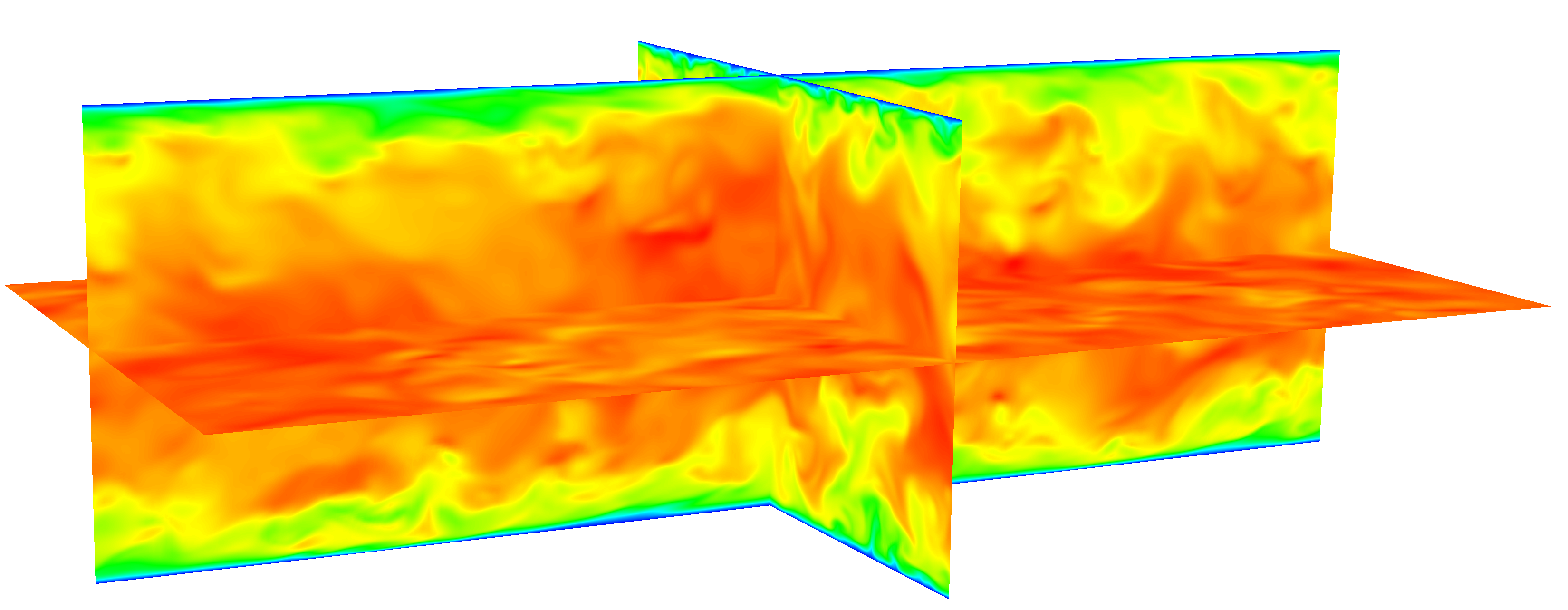
For $\rm Re_{\tau}=180$, we follow the setup in [5], in which the streamwise (i.e, the $x$-direction) and spanwise (i.e, the $z$-direction) lengths of the channel are set to $4\pi h$ and $4\pi h/3$, respectively, and the channel half-height is set to $h=1$. We consider twice as many grid points as in [5], with $E=5,832$ elements (an array of $18\times 18\times 18$ elements in the $x\times y\times z$ directions), of order $q=9$, for a total of ${\mathcal{N}}\approx 4.3$ million grid points. FOM statistics are collected over $1000$ convection time units (CTUs) and compared against the following two databases: (i) data in [52], which is collected over $3140$ CTUs and has $14.2$ million grid points; and (ii) data in [5], which has $2.1$ million grid points .

For $\rm Re_{\tau}=395$, we follow the setup in [6], in which the streamwise and spanwise lengths of the channel are set to $2\pi$ and $\pi$, respectively, and the channel half-height is set to $h=1$. We consider twice as many grid points as in [6], with $E=26,244$ elements (an array of $36\times 27\times 27$ elements in the $x\times y\times z$ directions), of order $q=9$, for a total of ${\mathcal{N}}\approx 20$ million grid points. FOM statistics are collected over $1500$ CTUs and compared against the data in [6], which has $9.5$ million grid points.

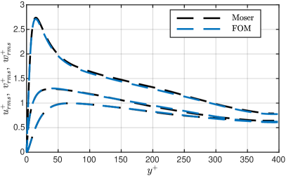
For both Reynolds numbers, the FOM is run until the solution reaches a statistically steady state prior to gathering statistics. To validate our FOM, in Fig. 5.2, for both $\rm Re_{\tau}$, we compare the FOM with the reference data with respect to the 2nd order turbulent statistics $u^{+}_{rms}$, $v^{+}_{rms}$, and $w^{+}_{rms}$ (in wall-units). For both $\rm Re_{\tau}$, we observe that the FOM 2nd order statistics are in good agreement with the published results.

Figure 5.2: FOM 2nd order statistics $u^{+}_{rms},~{}v^{+}_{rms}$, and $w^{+}_{rms}$ validation: (Left) $\rm Re_{\tau}=180$, comparison with [5, 52]. (Right) $\rm Re_{\tau}=395$, comparison with [6].

5.2 ROM Computational Setting

The POD basis functions are constructed using $K=2000$ uniformly distributed snapshots in the statistically steady state region, which spans $500$ CTUs for $\rm Re_{\tau}=180$, and $1000$ CTUs for $\rm Re_{\tau}=395$.

For each $\rm Re_{\tau}$, we compare the ROM performance for different ROM parameters in both the reproduction and the predictive regimes. The ROM offline phase, which includes the construction of the POD basis functions and reduced operators, is performed using NekROM on the UIUC cluster Delta. The ROM online phase, which includes loading the reduced operators and solving the ROM systems, is performed using Matlab on a workstation.

The implementation of the three Reg-ROMs (4.1–4.5) is similar: For a given filter order, $m$, and filter radius, $\delta$, all three Reg-ROMs involve computing the Cholesky factorization of the HOAF (3.3), that is $(I+\delta^{2m}(B^{-1}A)^{m})=R^{T}R$, and storing the inverse of the upper triangular matrix, $R^{-1}$. At each time step, a matrix multiplication $R^{-1}R^{-T}{\underline{u}}$ is performed to obtain the filtered ROM coefficients, ${\underline{\overline{u}}}$. The only difference in the particular Reg-ROM implementation is how ${\underline{\overline{u}}}$ is used in the Reg-ROM equation. We also emphasize that, because the most expensive part is to filter the ROM coefficients, the computational overhead is similar for all three Reg-ROMs.

5.3 Criteria

To evaluate the ROM performance, we use the FOM data as a benchmark, and the streamwise Reynolds normal stress $\langle u^{\prime}u^{\prime}\rangle$ and the Reynolds shear stress $\langle u^{\prime}v^{\prime}\rangle$, which are the two dominant terms in the Reynolds stress tensor, as criteria for accuracy evaluation. Specifically, we use the following formulas:

$$\varepsilon_{u^{\prime}u^{\prime}}\coloneqq\frac{\|\langle u^{\prime}u^{\prime}\rangle_{\text{r}}-\langle u^{\prime}u^{\prime}\rangle\|_{2}}{\|{\langle u^{\prime}u^{\prime}\rangle}\|_{2}},\quad\varepsilon_{u^{\prime}v^{\prime}}\coloneqq\frac{\|\langle u^{\prime}v^{\prime}\rangle_{\text{r}}-\langle u^{\prime}v^{\prime}\rangle\|_{2}}{\|{\langle u^{\prime}v^{\prime}\rangle}\|_{2}},$$ (5.1)

where $\langle u^{\prime}u^{\prime}\rangle$ and $\langle u^{\prime}v^{\prime}\rangle$ are the FOM Reynolds stresses, and $\langle u^{\prime}u^{\prime}\rangle_{\text{r}}$, $\langle u^{\prime}v^{\prime}\rangle_{\text{r}}$ are the ROM Reynolds stresses.

The FOM Reynolds stresses are defined as follows:

$$\langle u^{\prime}u^{\prime}\rangle \coloneqq\Bigl{\langle}\left(u-\langle u\rangle\right)^{2}\Bigr{\rangle}=\Bigl{\langle}u^{2}-2u\langle u\rangle+\langle u\rangle^{2}\Bigr{\rangle}=\Bigl{\langle}\langle u^{2}\rangle-\langle u\rangle^{2}\Bigr{\rangle},$$ (5.2)

$$\langle u^{\prime}v^{\prime}\rangle \coloneqq\Bigl{\langle}\left(u-\langle u\rangle\right)\left(v-\langle v\rangle\right)\Bigr{\rangle}$$

$$=\Bigl{\langle}uv-u\langle v\rangle-v\langle u\rangle+\langle u\rangle\langle v\rangle\Bigr{\rangle}=\Bigl{\langle}\langle uv\rangle-\langle u\rangle\langle v\rangle\Bigr{\rangle}.$$ (5.3)

The ROM Reynolds stresses are computed using (5.2)-(5.3), but with the ROM approximated solution (2.2):

$$\langle u^{\prime}u^{\prime}\rangle_{\text{r}} \coloneqq\Bigl{\langle}\langle u_{\text{r}}^{2}\rangle-\langle u_{\text{r}}\rangle^{2}\Bigr{\rangle},\quad\langle u^{\prime}v^{\prime}\rangle_{\text{r}}\coloneqq\Bigl{\langle}\langle u_{\text{r}}v_{\text{r}}\rangle-\langle u_{\text{r}}\rangle\langle v_{\text{r}}\rangle\Bigr{\rangle}.$$ (5.4)

In this paper, an angle bracket $\bigl{\langle}\cdot\bigr{\rangle}$ indicates an average over $x$, $z$, and $t$, and is defined as:

$$\langle u\rangle(y)=\frac{1}{TL_{x}L_{x}}\sum_{x,z,t}u(x,y,z,t),$$ (5.5)

where $T$ is the length of the time interval, $L_{x}$ is the dimension of the computational domain in the $x$-direction, $L_{z}$ is the dimension of the computational domain in the $z$-direction, $u$ is a scalar field, and a prime indicates perturbation from this average.

We note that using Equation 5.4 to compute ROM Reynolds stresses requires accessing the POD basis functions and reconstructing the ROM quantities $\langle u^{2}_{\text{r}}\rangle$, $\langle u_{\text{r}}v_{\text{r}}\rangle$, $\langle u_{\text{r}}\rangle^{2}$, and $\langle u_{\text{r}}\rangle\langle v_{\text{r}}\rangle$, which scale with the FOM dimension, ${\mathcal{N}}$. Thus, using Equation 5.4 to compute $\langle u^{\prime}u^{\prime}\rangle_{\text{r}}$ and $\langle u^{\prime}v^{\prime}\rangle_{\text{r}}$ is inefficient.

5.3.1 Efficient Offline-Online Reynolds-Stress Evaluation

To efficiently compute the ROM Reynolds stresses, we use an alternative approach, based on an offline-online splitting. First, we rewrite Equation 5.4 with the POD expansion:

$$\langle u^{\prime}u^{\prime}\rangle_{\text{r}} =\Bigl{\langle}\bigl{\langle}(\sum^{N}_{j=0}u_{\text{r},j}(t)\varphi_{j})(\sum^{N}_{k=0}u_{\text{r},k}(t)\varphi_{k})\bigr{\rangle}-\bigl{\langle}\sum^{N}_{j=0}u_{\text{r},j}(t)\varphi_{j}\bigr{\rangle}^{2}\Bigr{\rangle},$$

$$=\langle\sum^{N}_{j=0}\sum^{N}_{k=0}\langle u_{\text{r},j}(t)u_{\text{r},k}(t)\varphi_{j}\varphi_{k}\rangle-\left(\sum^{N}_{j=0}\langle u_{\text{r},j}(t)\varphi_{j}\rangle\right)\left(\sum^{N}_{k=0}\langle u_{\text{r},k}(t)\varphi_{k}\rangle\right)\rangle,$$

$$=\sum^{N}_{j=0}\sum^{N}_{k=0}\langle u_{\text{r},j}u_{\text{r},k}\rangle_{t}\langle\varphi_{j}\varphi_{k}\rangle_{xz}-\sum^{N}_{j=0}\sum^{N}_{k=0}\langle u_{\text{r},j}\rangle_{t}\langle u_{\text{r},k}\rangle_{t}\langle\varphi_{j}\rangle_{xz}\langle\varphi_{k}\rangle_{xz},$$ (5.6)

where $\varphi_{j}$ and $\varphi_{k}$ are the POD basis functions in the streamwise direction, and $\langle\cdot\rangle_{t}$ and $\langle\cdot\rangle_{xz}$ are the average operators in $t$ and the $x$-$z$ plane. Then, in the offline stage, for each $y$ coordinate, we compute and store $\langle\varphi_{j}\varphi_{k}\rangle_{xz}$ and $\langle\varphi_{j}\rangle_{xz}$ for all $j,~{}k=0,\ldots,N$. Finally, in the online stage, we compute $\langle{u_{\text{r},j}u_{\text{r},k}}\rangle_{t}$ and $\langle{u_{\text{r},j}}\rangle_{t}$ for all $j,~{}k=0,\ldots,N$. Thus, to construct the ROM streamwise Reynolds normal stress $\langle u^{\prime}u^{\prime}\rangle_{\text{r}}$ at a given point $y^{*}$, we use (5.6), which is independent of ${\mathcal{N}}$ and, thus, does not significantly increase the computational cost. The offline-online splitting for the ROM Reynolds shear stress $\langle u^{\prime}v^{\prime}\rangle_{\text{r}}$ can be derived similarly.

We also assess the ROM performance with the ROM-projection Reynolds stresses $\langle u^{\prime}u^{\prime}\rangle_{\text{Proj}}$ and $\langle u^{\prime}v^{\prime}\rangle_{\text{Proj}}$:

$$\langle u^{\prime}u^{\prime}\rangle_{\text{Proj}} \coloneqq\Bigl{\langle}\langle u_{\text{Proj}}^{2}\rangle-\langle u_{\text{Proj}}\rangle^{2}\Bigr{\rangle},$$ (5.7)

$$\langle u^{\prime}v^{\prime}\rangle_{\text{Proj}} \coloneqq\Bigl{\langle}\langle u_{\text{Proj}}v_{\text{Proj}}\rangle-\langle u_{\text{Proj}}\rangle\langle v_{\text{Proj}}\rangle\Bigr{\rangle},$$ (5.8)

where the projected solution onto the reduced space is defined as:

$${\bm{u}}_{\text{Proj}}=\bm{\varphi}_{0}+\sum^{N}_{j=0}\tilde{u}_{\text{Proj},j}\bm{\varphi}_{j}({\bf x}),~{}\text{and}~{}\tilde{u}_{\text{Proj},j}=(\bm{\varphi}_{j},{\bm{u}}-\bm{\varphi}_{0}).$$ (5.9)

The ROM-projection Reynolds stress can be computed using (5.6) but with $\langle\tilde{u}_{\text{Proj},j}\tilde{u}_{\text{Proj},j}\rangle_{t}$ and $\langle\tilde{u}_{\text{Proj},j}\rangle_{t}$ quantities, and is used to compute the error $\varepsilon_{u^{\prime}v^{\prime}}$ (5.1). The ROM projection represents the best theoretical approximation of the training data in the given ROM space, and we use it as a benchmark to assess the three Reg-ROMs.

5.4 Reproduction Regime

In this section, we perform a numerical investigation of the three Reg-ROMs: L-ROM (Section 4.1), EFR-ROM (Section 4.2), and the new TR-ROM (Section 4.3) in the reproduction regime, i.e., in the time interval in which the snapshots were collected, at $\rm Re_{\tau}=180$ (Section 5.4.1) and $\rm Re_{\tau}=395$ (Section 5.4.2). For comparison purposes, we include results for the G-ROM (Section 2.2) and the ROM projection, which represents the best theoretical approximation of the FOM solution in the given ROM space. The Reg-ROM accuracy is expected to be significantly higher than the G-ROM accuracy. To quantify the ROM accuracy, we use $\varepsilon_{u^{\prime}u^{\prime}}$ and $\varepsilon_{u^{\prime}v^{\prime}}$, which are the relative $\ell^{2}$ errors of the streamwise Reynolds normal stress $\langle u^{\prime}u^{\prime}\rangle$ and Reynolds shear stress $\langle u^{\prime}v^{\prime}\rangle$ defined in Equation 5.1.

In our numerical investigation, we also consider the following parameters: For all the ROMs, we utilize $10$ values for the ROM dimension, $N\in\{10,20,\ldots,$ $90,100\}$. For each Reg-ROM, we use four HOAF orders: $m=1$ (which corresponds to the classical DF (3.2)) and $m=2,3,4$ (which correspond to the HOAF (3.3)). For each $N$ and $m$ value, the values of the filter radius, $\delta$, are chosen as follows: For EFR-ROM and TR-ROM, $10$, $25$, and $10$ $\delta$ values are uniformly sampled from the intervals $[0.001,~{}0.01]$, $[0.01,0.1]$, and $[0.1,1]$, respectively. This yields a total of $43$ values for $\delta$ from the interval $[0.001,~{}1]$. In addition, we choose $4$ uniformly sampled values for the relaxation parameter, $\chi$, in the interval $[\Delta t=0.005,~{}1]$. We choose this $\chi$ range because $\chi=\mathcal{O}(\Delta t)$ is commonly used in EFR-ROM simulations [53, 18]. For L-ROM, we uniformly sample $15$ additional $\delta$ values from the interval $[0.1,~{}0.2]$, which yields a total of $56$ values for $\delta$ from the interval $[0.001,~{}1]$ for $\rm Re_{\tau}=180$. For $\rm Re_{\tau}=395$, $30$ additional $\delta$ values are uniformly sampled from the interval $[0.1,~{}0.3]$, which yields a total of $69$ values for $\delta$.

We emphasize that, in our Reg-ROM numerical investigation, we use four parameters: the ROM dimension, $N$, the filter order, $m$, the filter radius, $\delta$, and (for EFR-ROM and TR-ROM) the relaxation parameter, $\chi$. Thus, to ensure a clear comparison of the three Reg-ROMs, we fix the $\delta$ and $\chi$ parameters to their optimal values (i.e., the values that yield the most accurate Reynolds shear stress $\langle u^{\prime}v^{\prime}\rangle$ for each Reg-ROM), and plot $\varepsilon_{u^{\prime}v^{\prime}}$ for all the parameter values for $N$ and $m$. We note that we show only $\varepsilon_{u^{\prime}v^{\prime}}$ results for the following two reasons: (i) We find that $\varepsilon_{u^{\prime}u^{\prime}}$ behaves similarly to $\varepsilon_{u^{\prime}v^{\prime}}$. Specifically, $\varepsilon_{u^{\prime}u^{\prime}}$ is generally smaller than $\varepsilon_{u^{\prime}v^{\prime}}$ at $\rm Re_{\tau}=180$, and similar to $\varepsilon_{u^{\prime}v^{\prime}}$ at $\rm Re_{\tau}=395$. (ii) In turbulent channel flow investigations, the approximation of the Reynolds shear stress $\langle u^{\prime}v^{\prime}\rangle$ is more challenging than the approximation of streamwise Reynolds normal stress $\langle u^{\prime}u^{\prime}\rangle$. For the $\varepsilon_{u^{\prime}u^{\prime}}$ results, we refer reader to the dissertation [54]. For completeness, in the sensitivity study in Section 5.6, we include Reg-ROM results for all the $\delta$ and $\chi$ values.

Finally, in Section 5.4.3, we present a summary of the Reg-ROM comparison in the reproduction regime.

5.4.1 $\rm Re_{\tau}=180$

In Figure 5.3, we plot the relative $\ell^{2}$ error $\varepsilon_{u^{\prime}v^{\prime}}$ Equation 5.1 for different ROM dimensions, $N$, and filter orders, $m$, for the G-ROM, the ROM projection, and the three Reg-ROMs at $\rm Re_{\tau}=180$. Two sets of ROM-projection results are shown: The solid and the dotted lines represent the errors of $\langle u^{\prime}v^{\prime}\rangle_{\text{Proj}}$ (5.8) for the snapshot data and the FOM data, respectively. It is expected that the error $\varepsilon_{u^{\prime}v^{\prime}}$ for the snapshot data is smaller than the error for the FOM data, because the POD basis set is constructed using only $K=2000$ snapshots instead of using all the FOM solutions. For each Reg-ROM, the error is plotted for the optimal $\delta$ values and, for EFR-ROM and TR-ROM, for the optimal $\chi$ values.

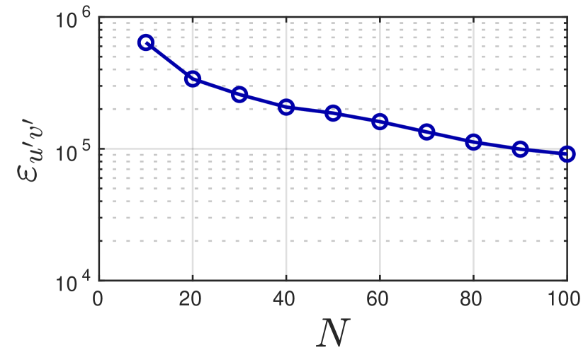
Figure 3(a) displays the G-ROM results. This plot shows that, for all $N$ values, the G-ROM results are very inaccurate. Even with $N=100$, G-ROM fails to reconstruct $\langle u^{\prime}v^{\prime}\rangle$ with an error of $\mathcal{O}(10^{5})$.

(a) G-ROM

(b) L-ROM

(c) EFR-ROM

(d) TR-ROM

Figure 5.3: The relative error $\varepsilon_{u^{\prime}v^{\prime}}$ Equation 5.1 of G-ROM, ROM projection, L-ROM, EFR-ROM, and TR-ROM in the reproduction regime at $\rm Re_{\tau}=180$ for different $N$ and $m$ values with optimal $\delta$ and $\chi$ values.

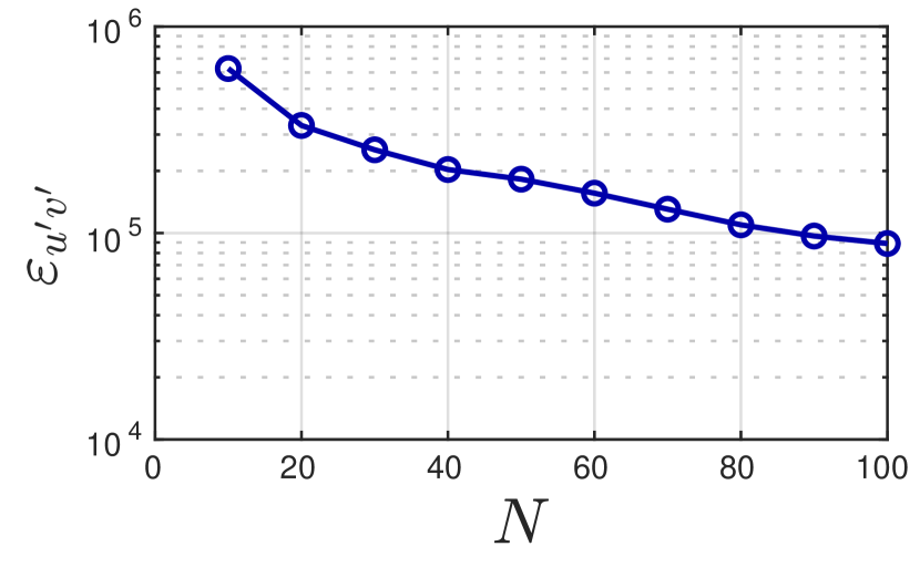
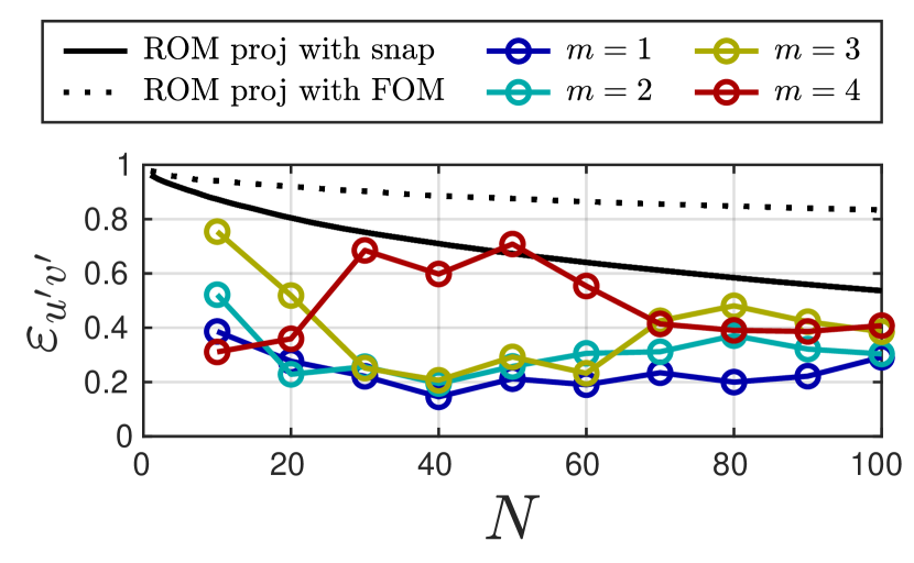
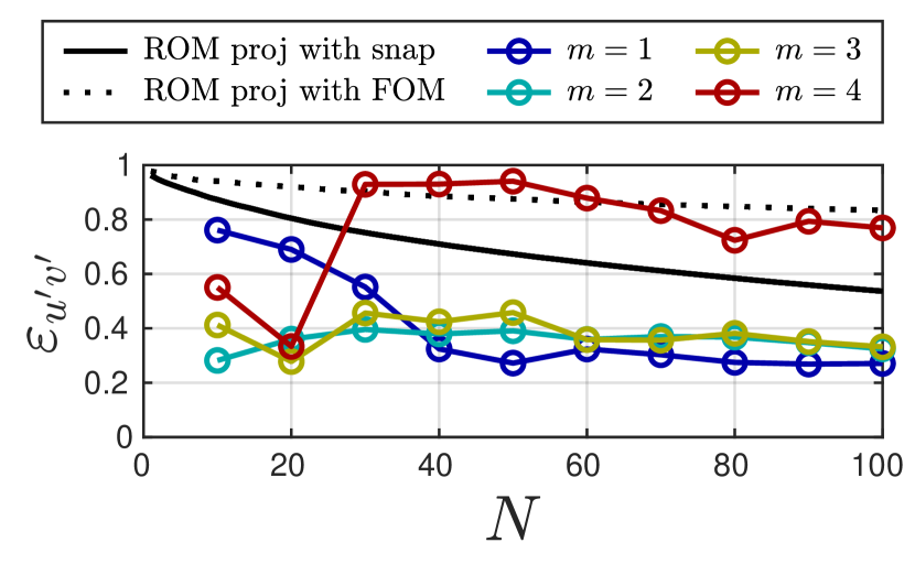
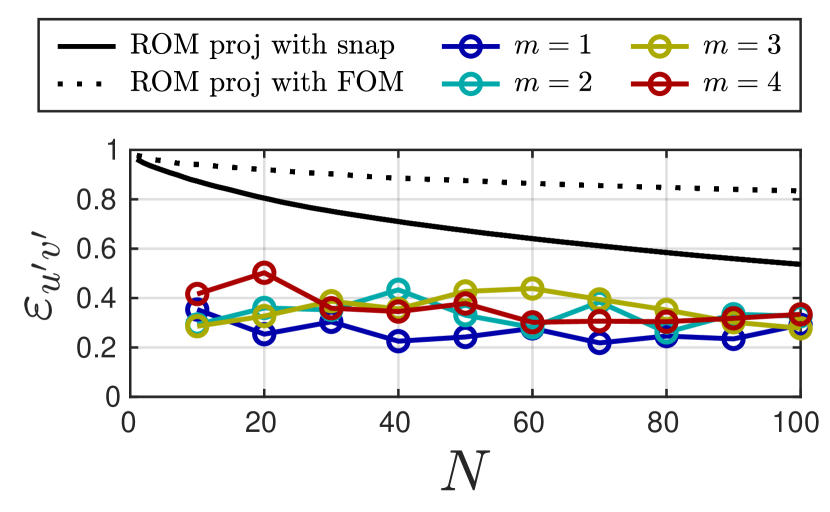
Figure 3(b) displays the L-ROM results for each $N$ and $m$ with the optimal $\delta$, along with the results of the ROM projection for comparison purposes. For $N\geq 30$, $m=1$ yields the most accurate results, achieving an error of $15\%$ for $N=40$. Conversely, for $N\leq 20$, a higher-order filter yields better results. Specifically, $m=4$ achieves an error of $31\%$ for $N=10$ and $m=2$ achieves an error of $23\%$ for $N=20$. With the exception of $(N,m)=(50,4)$, L-ROM is more accurate than the ROM projection.

Figure 3(c) displays the EFR-ROM results for each $N$ and $m$ with the optimal $\chi$ and $\delta$ values, along with the results of the ROM projection for comparison purposes. For $N\geq 40$, $m=1$ yields the most accurate results, achieving an error of $27\%$ for $N=90$. Conversely, for $N\leq 30$, a higher-order filter yields better results. Specifically, $m=2$ achieves an error of $28\%$ and $40\%$ for $N=10$ and $N=30$, respectively. Additionally, $m=3$ achieves an error of $45\%$ for $N=20$. EFR-ROM is more accurate than the ROM projection for all $N$ with $m=1,~{}2,~{}3$. With $m=4$, it is only more accurate than the ROM projection for $N\leq 30$.

Figure 3(d) displays the TR-ROM results for each $N$ and $m$ with the optimal $\chi$ and $\delta$ values, along with the results of the ROM projection for comparison purposes. For $20\leq N\leq 90$, $m=1$ yields the most accurate results, achieving an error of $22\%$ for $N=70$. For $N=10$ and $N=100$, $m=3$ yields the most accurate results, achieving an error of $29\%$ and $28\%$, respectively. In addition, TR-ROM is more accurate than the ROM projection for all $N$ and $m$ values.

5.4.2 $\rm Re_{\tau}=395$

In Figure 5.4, we plot the relative $\ell^{2}$ error $\varepsilon_{u^{\prime}v^{\prime}}$ Equation 5.1 for different $N$ and $m$ values for the G-ROM, the ROM projection, and the three Reg-ROMs at $\rm Re_{\tau}=395$. Two sets of ROM-projection results for the snapshot data and the FOM data are shown. Note that the error $\varepsilon_{u^{\prime}v^{\prime}}$ for the snapshot data at $\rm Re_{\tau}=395$ is larger (approximately $70\%$) than the corresponding results at $\rm Re_{\tau}=180$ (approximately $52\%$). This difference is expected because the $\rm Re_{\tau}=395$ solution is more turbulent and, as a result, requires a larger number of modes to achieve a satisfactory approximation. For each Reg-ROM, the error is plotted for the optimal $\delta$ values and, for EFR-ROM and TR-ROM, for the optimal $\chi$ values.

(a) G-ROM

(b) L-ROM

(c) EFR-ROM

(d) TR-ROM

Figure 5.4: The relative error $\varepsilon_{u^{\prime}v^{\prime}}$ Equation 5.1 of G-ROM, ROM projection, L-ROM, EFR-ROM, and TR-ROM in the reproduction regime at $\rm Re_{\tau}=395$ for different $N$ and $m$ values with optimal $\delta$ and $\chi$ values.

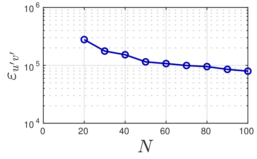
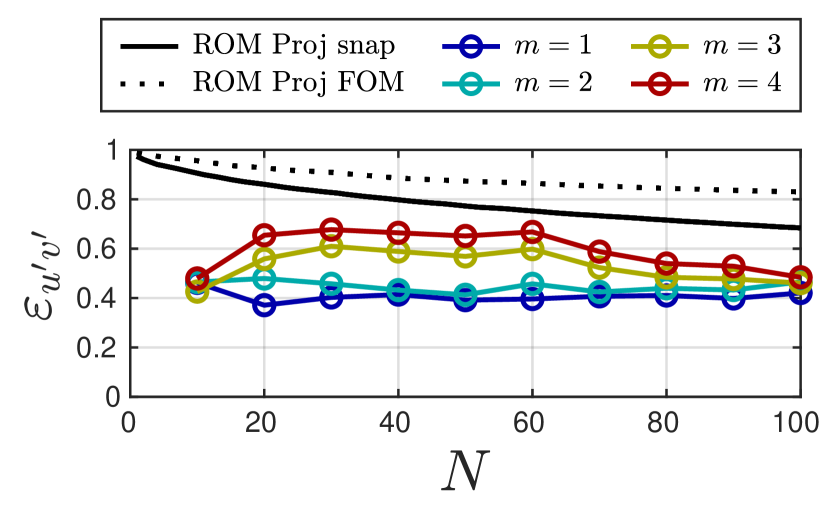
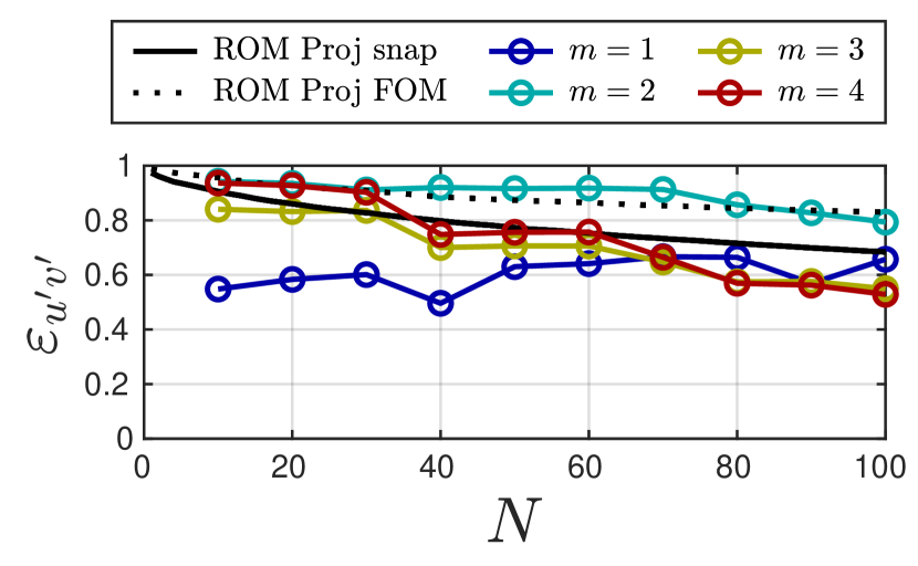
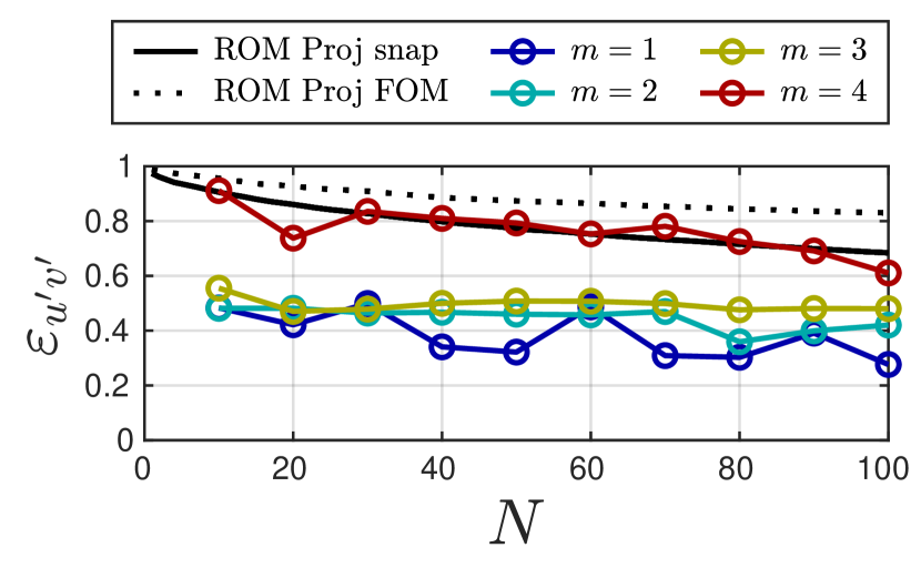
Figure 4(a) displays the G-ROM results. Just as in Section 5.4.1, for all $N$ values, the G-ROM results are very inaccurate. Even with $N=100$, $\varepsilon_{u^{\prime}v^{\prime}}$ is still about $\mathcal{O}(10^{5})$.

Figure 4(b) displays the L-ROM results for each $N$ and $m$ with the optimal $\delta$ values, along with the results of the ROM projection for comparison purposes. For all $N$ and $m$ values, the error is much higher than the error for $\rm Re_{\tau}=180$. For $N\geq 20$, the most accurate results are achieved with $m=1$, with an error of $37\%$ for $N=40$. For $N=10$, $m=3$ achieves an error of $43\%$. Compared to the ROM projection, L-ROM is more accurate for all values of $N$ and $m$.

Figure 4(c) displays the EFR-ROM results for each $N$ and $m$ with the optimal $\chi$ and $\delta$ values, along with the results of the ROM projection for comparison purposes. These results are qualitatively different from the EFR-ROM results for $\rm Re_{\tau}=180$. For $N\leq 60$, $m=1$ yields the most accurate results and achieves an error of $50\%$ for $N=40$. For $N\geq 70$, higher-order filter yields better results. Specifically, $m=4$ achieves an error of $53\%$ for $N=100$. Moreover, EFR-ROM is found to be more accurate than the ROM projection for all $N$ with $m=1$ and for $N\geq 60$ with $m=3,~{}4$. With $m=2$, EFR-ROM has a similar level of accuracy as the ROM projection.

Figure 4(d) displays the TR-ROM results for each $N$ and $m$ with the optimal $\chi$ and $\delta$ values, along with the results of the ROM projection for comparison purposes. For almost all $N$ values, $m=1$ yields the most accurate results, achieving an error of around $28\%$ for $N=100$. These results also show that $m=2$ and $m=3$ yield similar results, while $m=4$ is found to be the least accurate. Moreover, TR-ROM is found to be more accurate than the ROM projection for all $N$ and $m$ values.

5.4.3 Summary

Overall, our numerical investigation in the reproduction regime yields the following general conclusions:

All three Reg-ROMs are significantly more accurate than the standard G-ROM. In fact, with respect to several second-order turbulence statistics, the errors of the three Reg-ROMs equipped with carefully tuned spatial filtering are much lower than the projection error.

Finally, our numerical investigation demonstrates that, for $\rm Re_{\tau}=180$, all three Reg-ROMs with $m=1$ (i.e., low-order filtering) consistently produce the most accurate results for large $N$ values, while a higher-order filter is more effective for low $N$ values. For $\rm Re_{\tau}=395$, L-ROM and TR-ROM with $m=1$ yield the most accurate results for all $N$ values, while EFR-ROM yields the most accurate results for low $N$ values with $m=1$, and for high $N$ values with $m=3,~{}4$.

To facilitate the comparison of the three Reg-ROMs, in Table 1, we rank them based on the error $\varepsilon_{u^{\prime}v^{\prime}}$ and $\varepsilon_{u^{\prime}u^{\prime}}$ achieved for the $N$ and $m$ values investigated. Specifically, for both Reynolds numbers, we list the Reg-ROMs’ rank, the lowest $\varepsilon_{u^{\prime}v^{\prime}}$, the corresponding $\varepsilon_{u^{\prime}u^{\prime}}$, the ROM dimension $N$ and the filter order $m$ for which the lowest $\varepsilon_{u^{\prime}v^{\prime}}$ is achieved. The results in Table 1 yield the following conclusions:

For $\rm Re_{\tau}=180$, TR-ROM is the most accurate model with $\varepsilon_{u^{\prime}v^{\prime}}\approx 22\%$ and $\varepsilon_{u^{\prime}u^{\prime}}\approx 16\%$, followed by EFR-ROM and L-ROM. For $\rm Re_{\tau}=395$, TR-ROM is still the most accurate model with $\varepsilon_{u^{\prime}v^{\prime}}\approx 28\%$ and $\varepsilon_{u^{\prime}u^{\prime}}\approx 26\%$, followed by L-ROM and EFR-ROM. In addition, we find $\varepsilon_{u^{\prime}u^{\prime}}$ is smaller compared to $\varepsilon_{u^{\prime}v^{\prime}}$ except for L-ROM for $\rm Re_{\tau}=180$ and $\varepsilon_{u^{\prime}u^{\prime}}$ has similar level of accuracy as $\varepsilon_{u^{\prime}v^{\prime}}$ for $\rm Re_{\tau}=395$. Moreover, the results in Table 1 also show that $m=1$ (i.e., low-order filtering) yields the most accurate results. Finally, these results show that TR-ROM requires large $N$ values to achieve its best accuracy, whereas L-ROM yields best accuracy with small $N$. For EFR-ROM, large $N$ is required for $\rm Re_{\tau}=180$, and small $N$ is required for $\rm Re_{\tau}=395$.

Table 1: Reg-ROM accuracy ranking in the reproduction regime for $\rm Re_{\tau}=180$ (top rows) and $395$ (bottom rows). The following parameters are listed: Reg-ROMs’ rank, the lowest $\varepsilon_{u^{\prime}v^{\prime}}$, the corresponding $\varepsilon_{u^{\prime}u^{\prime}}$, the ROM dimension $N$ and the filter order $m$ for which the lowest $\varepsilon_{u^{\prime}v^{\prime}}$ is achieved.

$\rm Re_{\tau}=180$	L-ROM	EFR-ROM	TR-ROM
Rank	3	2	1
$\varepsilon_{u^{\prime}v^{\prime}}$	$\approx 19\%$	$\approx 27\%$	$\approx 22\%$
$\varepsilon_{u^{\prime}u^{\prime}}$	$\approx 37.5\%$	$\approx 13\%$	$\approx 16\%$
N	$40$	$90$	$70$
$m$	1	1	1
$\rm Re_{\tau}=395$	L-ROM	EFR-ROM	TR-ROM
Rank	2	3	1
$\varepsilon_{u^{\prime}v^{\prime}}$	$\approx 37\%$	$\approx 50\%$	$\approx 28\%$
$\varepsilon_{u^{\prime}u^{\prime}}$	$\approx 40\%$	$\approx 40\%$	$\approx 26\%$
N	$20$	$40$	$100$
$m$	1	1	1

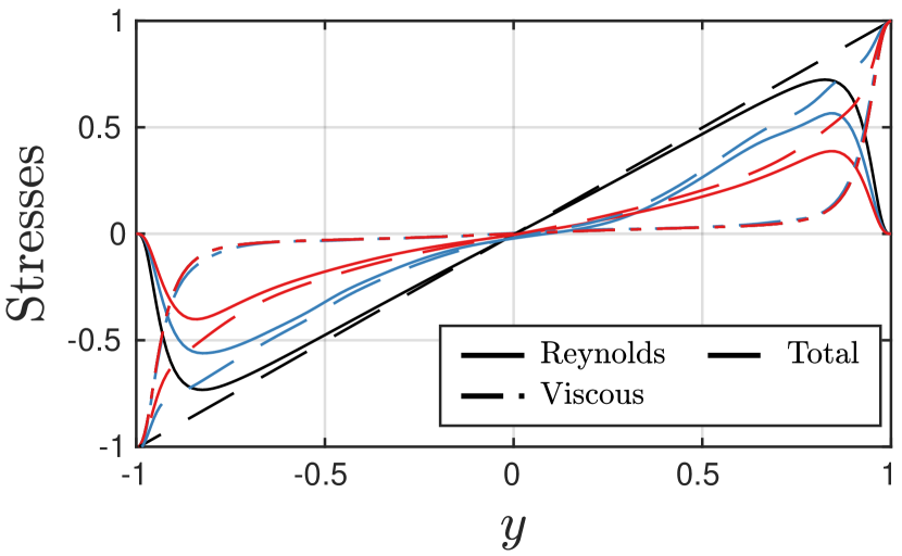
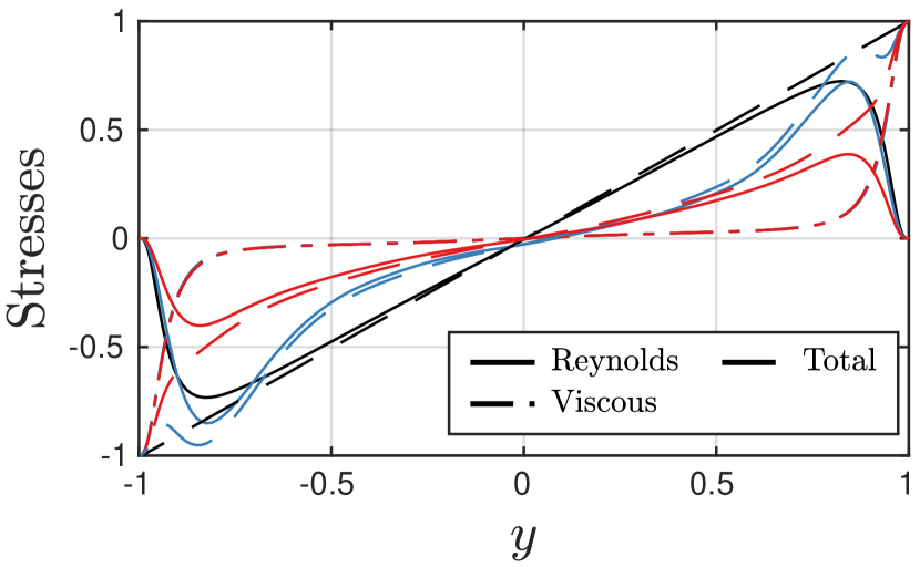
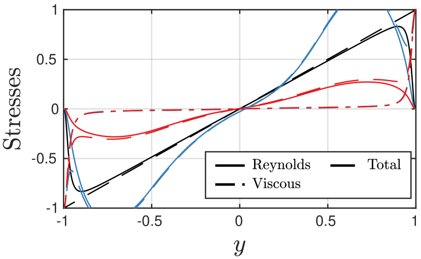
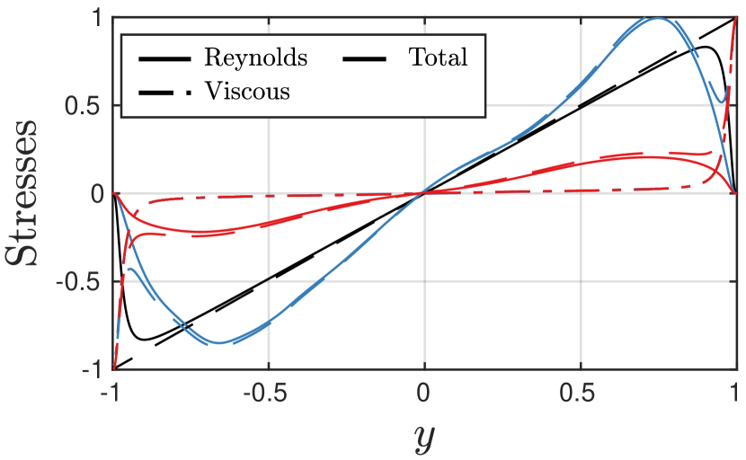
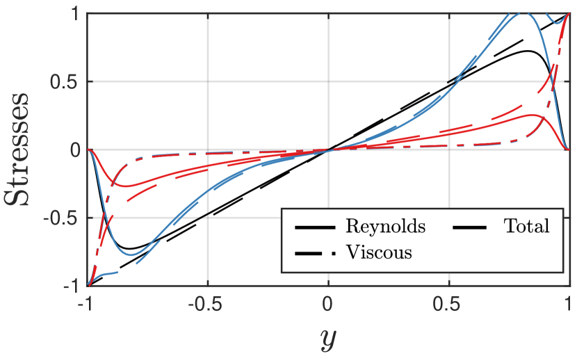
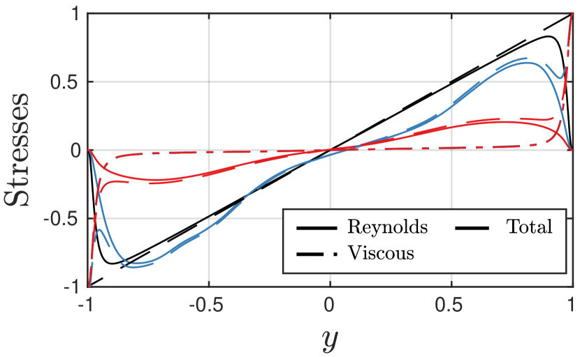
In Fig. 5.5, we compare the total, viscous, and Reynolds shear stresses of the optimal Reg-ROMs (listed in Table 1) along with the results of the FOM and the ROM projection in the reproduction regime for $\rm Re_{\tau}=180$ and $\rm Re_{\tau}=395$. The total shear stress $\tau(y)$ is the sum of the viscous shear stress $\rho\,\nu\,d\langle u\rangle/dy$ and the Reynolds shear stress $-\rho\,\langle uv\rangle$, and its distribution is linear [55]. In each model, the three shear stresses are normalized with the model’s wall shear stress $\tau_{w}\equiv\rho\,\nu\,\left(d\langle u\rangle/dy\right)_{y=-1}$.

In terms of the viscous shear stress, the results of the three Reg-ROMs are in good agreement with those of the FOM and the ROM projection for both $\rm Re_{\tau}$. In terms of the Reynolds shear stress, for $\rm Re_{\tau}=180$, we observe that the L-ROM result is smaller than the FOM result. On the other hand, the results of the EFR-ROM and the TR-ROM are similar, and both have higher values in the boundary layer and lower values outside the boundary layer compared to the FOM. Notice that both the EFR-ROM and the TR-ROM are able to capture the slope of the Reynolds shear stress. For $\rm Re_{\tau}=395$, we find that the result of the TR-ROM is the best, followed by L-ROM and EFR-ROM. Moreover, although the results of the Reg-ROMs are not perfect, we find that the results are much better than the ROM projection. This also indicates that $N=100$ POD bases are not able to reconstruct the Reynolds stress. Finally, as a result of the discrepancy in the Reynolds shear stress, the total shear stress is not linear in all three Reg-ROMs for both $\rm Re_{\tau}$.

(a) L-ROM, $\rm Re_{\tau}=180$

(b) L-ROM, $\rm Re_{\tau}=395$

(c) EFR-ROM, $\rm Re_{\tau}=180$

(d) EFR-ROM, $\rm Re_{\tau}=395$

(e) TR-ROM, $\rm Re_{\tau}=180$

(f) TR-ROM, $\rm Re_{\tau}=395$

Figure 5.5: Comparison of the total, viscous, and Reynolds shear stresses of the FOM (black), the ROM projection (red), and the optimal Reg-ROMs, listed in Table 1 (blue) in the reproduction regime for $\rm Re_{\tau}=180$ (left) and $\rm Re_{\tau}=395$ (right). The total shear stress is the sum of the viscous and the Reynolds shear stress.

5.5 Predictive Regime

In this section, we perform a numerical investigation of the three Reg-ROMs: L-ROM (Section 4.1), EFR-ROM (Section 4.2), and the new TR-ROM (Section 4.3) for the predictive regime, on a time interval that is $500$ CTUs larger than the time interval on which snapshots were collected, at $\rm Re_{\tau}=180$ (Section 5.5.1) and $\rm Re_{\tau}=395$ (Section 5.5.2). Hence, $1000$ CTU and $1500$ CTU time windows are considered for $\rm Re_{\tau}=180$ and $395$, respectively. For comparison purposes, we include results for the G-ROM (Section 2.2) and the ROM projection. To quantify the ROM accuracy, we use $\varepsilon_{u^{\prime}u^{\prime}}$ and $\varepsilon_{u^{\prime}v^{\prime}}$, which are the relative $\ell^{2}$ error of $\langle u^{\prime}u^{\prime}\rangle$ and $\langle u^{\prime}v^{\prime}\rangle$ defined in Equation 5.1. In order to measure the accuracy of the predicted $\langle u^{\prime}u^{\prime}\rangle$ and $\langle u^{\prime}v^{\prime}\rangle$, an additional $500$ CTUs of FOM simulations are performed for both $\rm Re_{\tau}$. For the $\varepsilon_{u^{\prime}u^{\prime}}$ results, we refer reader to the dissertation [54].

In our numerical investigation, we use the same parameter values for $N$ and $m$ as the values used in Section 5.4. For each $N$ and $m$ values, we plot $\varepsilon_{u^{\prime}v^{\prime}}$ with $(\delta,~{}\chi)_{\text{recon}}$, that is, the $\delta$ and $\chi$ parameter values that were found to be optimal in the reproduction regime in Section 5.4. We emphasize that our strategy is different from that used in Section 5.4: Instead of optimizing the $\delta$ and $\chi$ values on the entire predictive time interval, we use the values that were optimized over the shorter time interval of the reproduction regime. Thus, in this section, we are investigating the predictive power of both the Reg-ROMs and their associated parameters.

Finally, in Section 5.5.3, we present a summary of the Reg-ROM comparison in the predictive regime.

5.5.1 $\rm Re_{\tau}=180$

(a) G-ROM

(b) L-ROM

(c) EFR-ROM

(d) TR-ROM

Figure 5.6: The relative error $\varepsilon_{u^{\prime}v^{\prime}}$ Equation 5.1 of G-ROM, ROM projection, L-ROM, EFR-ROM, and TR-ROM in the predictive regime at $\rm Re_{\tau}=180$ for different $N$ and $m$ values with optimal $\delta$ and $\chi$ values optimized in the reproduction regime.

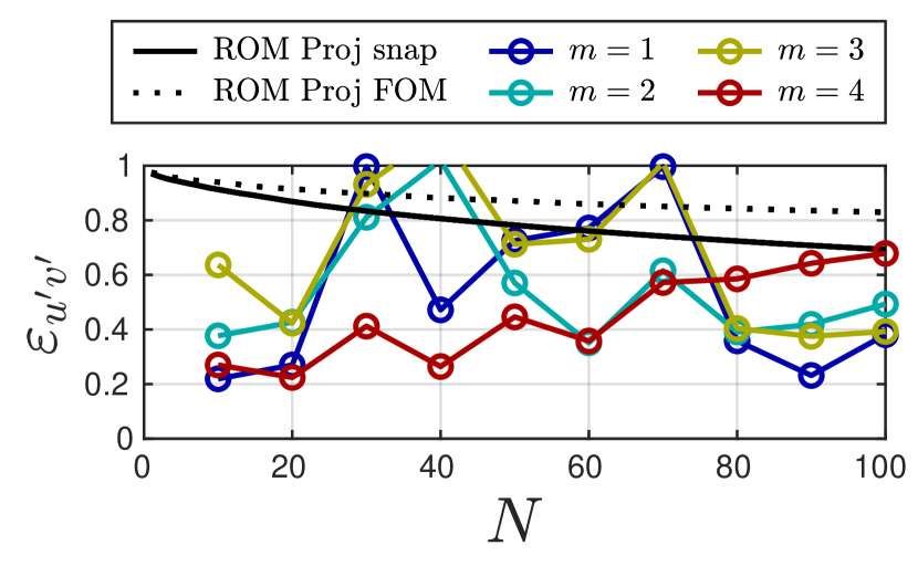
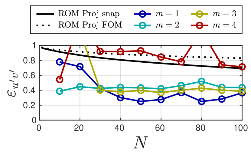
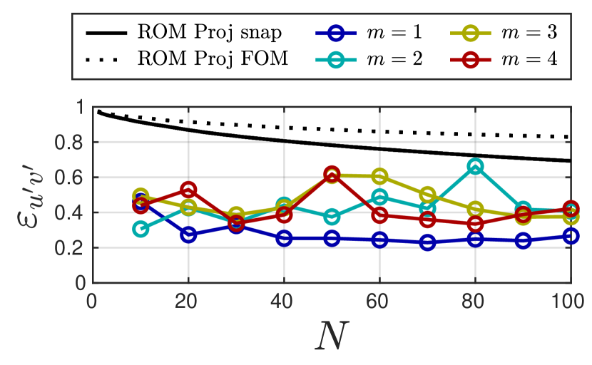
In Figure 5.6, we plot the relative $\ell^{2}$ error $\varepsilon_{u^{\prime}v^{\prime}}$ Equation 5.1 for different $N$ and $m$ values for the G-ROM, the ROM projection, and the three Reg-ROMs at $\rm Re_{\tau}=180$. We emphasize that, to test the predictive capabilities of the Reg-ROM parameters, we plot the error for $(\delta,~{}\chi)_{\text{recon}}$ that were optimized in the reproduction regime (Section 5.4.1).

Figure 6(a) displays the G-ROM results. As in the reproduction regime, for all $N$ values, the G-ROM results are very inaccurate.

Figure 6(b) displays the L-ROM results for each $N$ and $m$ with $\delta_{\text{recon}}$ along with the ROM projection results for comparison purposes. For $N=10$ and $N\geq 80$, $m=1$ yields the most accurate results, achieving an error of $22\%$ for $N=10$. For $20\leq N\leq 70$, $m=4$ yields the most accurate results, achieving an error of $22\%$ for $N=20$. For the majority of $N$ and $m$ values, except for the $(m,N)$ values $(1,30)$, $(1,70)$, $(2,40)$, $(3,30)$, $(3,40)$, and $(3,70)$, L-ROM is more accurate than the ROM projection.

However, $\varepsilon_{u^{\prime}v^{\prime}}$ exhibits a higher sensitivity to changes in $N$ across all $m$ values compared to the results observed in the reproduction regime (as discussed in Section 5.4.1).

Figure 6(c) displays the EFR-ROM results for each $N$ and $m$ with $(\delta,~{}\chi)_{\text{recon}}$ along with the ROM projection results for comparison purposes. For $N\leq 30$, higher-order filter yields better results. Specifically, for $N=10$ and $N=20$, EFR-ROM achieves an error of $39\%$ and $45\%$, respectively, with $m=2$. Additionally, for $N=30$, EFR-ROM achieves an error of $40\%$ with $m=3$. For $N\geq 40$, $m=1$ yields the most accurate results, achieving an error of $25\%$ for $N=80$. Compared to the ROM projection, EFR-ROM is more accurate for $m\leq 3$, except for $N=10$ and $N=20$ with $m=3$. For $m=4$, EFR-ROM is not accurate and its level of accuracy is similar to that of the ROM projection.

Figure 6(d) displays the TR-ROM results for each $N$ and $m$ with $(\delta,~{}\chi)_{\text{recon}}$ along with the ROM projection results for comparison purposes. For $N=10$, $m=2$ yields the lowest error of $30\%$. For $N\geq 20$, $m=1$ yields the best results, achieving an error of $23\%$ for $N=70$. TR-ROM is more accurate than the ROM projection for all $N$ and $m$ values.

5.5.2 $\rm Re_{\tau}=395$

In Figure 5.7, we plot the relative $\ell^{2}$ error $\varepsilon_{u^{\prime}v^{\prime}}$ for different $N$ and $m$ values for the G-ROM, the ROM projection, and the three Reg-ROMs at $\rm Re_{\tau}=395$. We emphasize that, to test the predictive capabilities of the Reg-ROM parameters, we plot the error for $(\delta,~{}\chi)_{\text{recon}}$ that were optimized in the reproduction regime (Section 5.4.2).

(a) G-ROM

(b) L-ROM

(c) EFR-ROM

(d) TR-ROM

Figure 5.7: The relative error $\varepsilon_{u^{\prime}v^{\prime}}$ Equation 5.1 of G-ROM, ROM projection, L-ROM, EFR-ROM, and TR-ROM in the predictive regime at $\rm Re_{\tau}=395$ for different $N$ and $m$ values with optimal $\delta$ and $\chi$ values optimized in the reproduction regime.

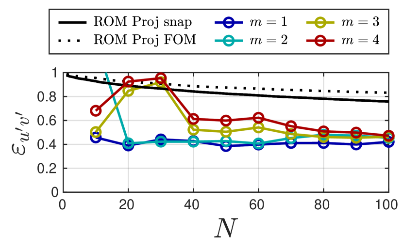
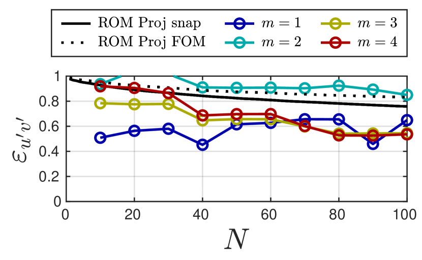
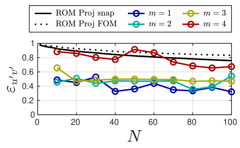
Figure 7(a) displays the G-ROM results. Just as in Section 5.5.1, for all $N$ values, the G-ROM results are very inaccurate with an error of $\mathcal{O}(10^{5})$ for $N=100$.

Figure 7(b) displays the L-ROM results for each $N$ and $m$ with $\delta_{\text{recon}}$, along with the ROM projection results for comparison purposes. For almost all $N$ values, except for $N=30$ and $N=40$, $m=1$ yields the most accurate results, achieving an error of $39\%$ with $N=20$. For $m=3$ and $m=4$, the accuracy of the L-ROM is improved as $N$ increases but is still larger than the $m=1$ case. Compared to the ROM projection, L-ROM is more accurate except for the $(m,N)$ pairs $(2,10),(3,30)$, $(4,20)$, and $(4,30)$.

Figure 7(c) displays the EFR-ROM results for each $N$ and $m$ with $(\delta,~{}\chi)_{\text{recon}}$ along with the ROM projection results for comparison purposes. For $N\leq 60$, $m=1$ yields the most accurate results, achieving an error of $45\%$ with $N=40$. For $N\geq 70$, except for $N=90$, a higher-order filter yields better results. Specifically, $m=4$ achieves an error of $53\%$ with $N=80$. For $N=90$, $m=1$ achieves an error of $46\%$. Compared to the ROM projection, EFR-ROM is more accurate for all $N$ values and $m=1,~{}3,~{}4$. For $m=2$, the EFR-ROM’s level of accuracy is similar to that of the ROM projection.

Figure 7(d) displays the TR-ROM results for each $N$ and $m$ with $(\delta,~{}\chi)_{\text{recon}}$, along with the ROM projection results for comparison purposes. For all $N$ values except $N=10$ and $N=30$, $m=1$ yields the most accurate results, achieving an error of around $32\%$ for $N=100$. These results also show that $m=2$ and $m=3$ yield similar accuracy, and $m=4$ is the least accurate. TR-ROM is more accurate than the ROM projection for all $N$ and $m$ values, except for the $(m,N)$ pairs $(4,50)$ and $(4,60)$.

5.5.3 Summary

Overall, our numerical investigation in the predictive regime yields the following general conclusions:

All three Reg-ROMs are significantly more accurate than the standard G-ROM.

In fact, with respect to several second-order turbulence statistics, the errors of the three Reg-ROMs equipped with carefully tuned spatial filtering are much lower than the projection error.

Finally, our numerical investigation demonstrates that, for $\rm Re_{\tau}=180$, EFR-ROM and TR-ROM with $m=1$ (i.e., low-order filtering) consistently produce the most accurate results for large $N$ values, while a higher-order filter is more effective for low $N$ values. In addition, L-ROM is sensitive to changes in $N$ for all $m$ values. For $\rm Re_{\tau}=395$, L-ROM and TR-ROM with $m=1$ yield the most accurate results for all $N$ values, while EFR-ROM yields the most accurate results for low $N$ values for $m=1$, and high $N$ values for $m=3,4$.

To facilitate the comparison of the three Reg-ROMs, in Table 2, we rank them based on the lowest error achieved for the $N$ and $m$ values investigated. Specifically, for both Reynolds numbers, we list the Reg-ROMs’ rank, the lowest $\varepsilon_{u^{\prime}v^{\prime}}$, the corresponding $\varepsilon_{u^{\prime}u^{\prime}}$, the ROM dimension $N$ and the filter order $m$ for which the lowest $\varepsilon_{u^{\prime}v^{\prime}}$ is achieved. The results in Table 2 yield the following conclusions:

Table 2: Reg-ROM accuracy ranking in the predictive regime for $\rm Re_{\tau}=180$ (top rows) and $395$ (bottom rows). The following parameters are listed: Reg-ROMs’ rank, the lowest $\varepsilon_{u^{\prime}v^{\prime}}$ with $\delta_{\text{recon}}$, the corresponding $\varepsilon_{u^{\prime}u^{\prime}}$, the ROM dimension $N$ and the filter order $m$ for which the lowest $\varepsilon_{u^{\prime}v^{\prime}}$ with $\delta_{\text{recon}}$ is achieved.

$\rm Re_{\tau}=180$	L-ROM	EFR-ROM	TR-ROM
Rank	2	3	1
$\varepsilon_{u^{\prime}v^{\prime}}$	$\approx 22\%$	$\approx 25\%$	$\approx 23\%$
$\varepsilon_{u^{\prime}u^{\prime}}$	$\approx 23\%$	$\approx 26\%$	$\approx 9\%$
N	$10$	$80$	$70$
Filter order $m$	1	1	1
$\rm Re_{\tau}=395$	L-ROM	EFR-ROM	TR-ROM
Rank	2	3	1
$\varepsilon_{u^{\prime}v^{\prime}}$	$\approx 39\%$	$\approx 45\%$	$\approx 32\%$
$\varepsilon_{u^{\prime}u^{\prime}}$	$\approx 39\%$	$\approx 36\%$	$\approx 30\%$
N	$50$	$40$	$100$
Filter order $m$	$1$	$1$	$1$

For $\rm Re_{\tau}=180$, TR-ROM is the most accurate model with $\varepsilon_{u^{\prime}v^{\prime}}\approx 23\%$ and $\varepsilon_{u^{\prime}u^{\prime}}\approx 9\%$, followed by L-ROM and EFR-ROM. For $\rm Re_{\tau}=395$, TR-ROM is still the most accurate model with $\varepsilon_{u^{\prime}v^{\prime}}\approx 32\%$ and $\varepsilon_{u^{\prime}u^{\prime}}\approx 30\%$, followed by EFR-ROM and L-ROM. In addition, the results in Table 2 also show that $m=1$ (i.e., low-order filtering) yields the most accurate results. Moreover, these results show that TR-ROM requires large $N$ values to achieve its best accuracy, whereas L-ROM yields best accuracy with small $N$. For EFR-ROM, large $N$ is required for $\rm Re_{\tau}=180$, and small $N$ is required for $\rm Re_{\tau}=395$.

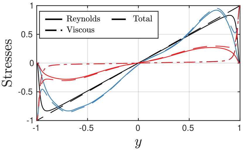
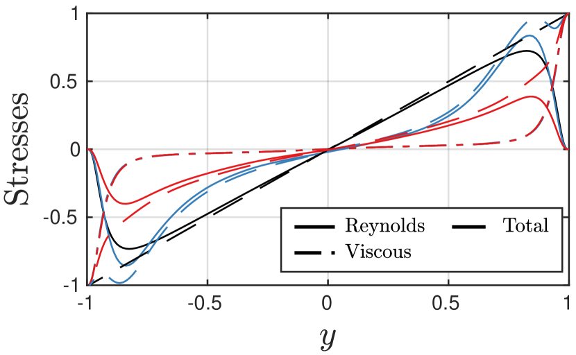
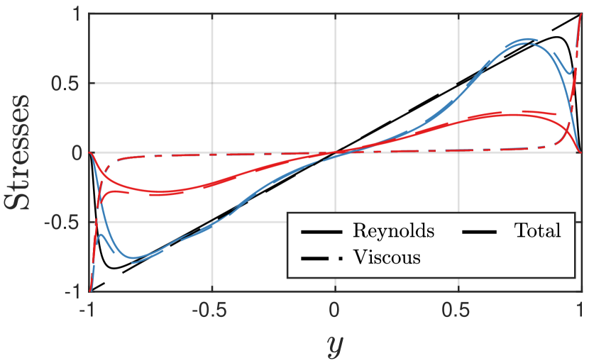
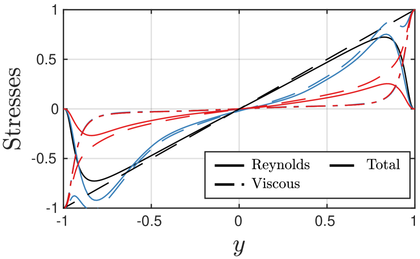
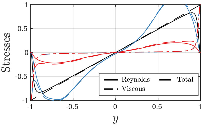
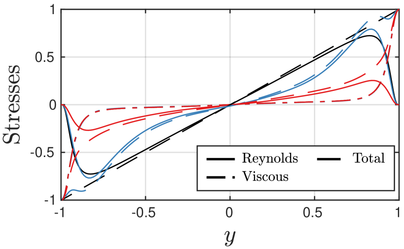
Similarly to the reproduction regime (Fig. 5.5), in Fig. 5.8, we compare the total, viscous, and the Reynolds shear stresses of the optimal Reg-ROMs (listed in Table 2) along with the results of the FOM and the ROM projection in the predictive regime for $\rm Re_{\tau}=180$ and $\rm Re_{\tau}=395$.

In terms of the viscous shear stress, the results of the three Reg-ROMs are in good agreement with those of the FOM and the ROM projection for both $\rm Re_{\tau}$. In terms of the Reynolds shear stress, we find that TR-ROM yields the most accurate results for both $\rm Re_{\tau}$ and the L-ROM is better than the EFR-ROM for $\rm Re_{\tau}=180$. For $\rm Re_{\tau}=395$, L-ROM and EFR-ROM perform similarly. In addition, from the results of the ROM projection, we find that $N=100$ POD basis functions are insufficient to reconstruct the Reynolds shear stress accurately. Finally, as a results of the discrepancy in the Reynolds shear stress, the total shear stress is not linear in all three Reg-ROMs for both $\rm Re_{\tau}$.

(a) L-ROM, $\rm Re_{\tau}=180$

(b) L-ROM, $\rm Re_{\tau}=395$

(c) EFR-ROM, $\rm Re_{\tau}=180$

(d) EFR-ROM, $\rm Re_{\tau}=395$

(e) TR-ROM, $\rm Re_{\tau}=180$

(f) TR-ROM, $\rm Re_{\tau}=395$

Figure 5.8: Comparison of the total, viscous, and Reynolds shear stresses of the FOM (black), the ROM projection (red), and the optimal Reg-ROMs, listed in Table 2 (blue) in the predictive regime for $\rm Re_{\tau}=180$ (left) and $\rm Re_{\tau}=395$ (right). The total shear stress is the sum of the viscous and the Reynolds shear stress.

Next, we discuss the potential issues that preclude Reg-ROMs from getting more accurate Reynolds shear stress.

From Figs. 5.3–5.7, we found that $\varepsilon_{u^{\prime}v^{\prime}}$ of the ROM projection has at least $55\%$ errors for $\rm Re_{\tau}=180$, and $70\%$ errors for $\rm Re_{\tau}=395$. This indicates the poor approximation capability of the reduced basis functions for the Reynolds shear stress $\langle u^{\prime}v^{\prime}\rangle$. With this approximation error, it is not surprising to find that $\varepsilon_{u^{\prime}v^{\prime}}$ of Reg-ROMs is not below $10\%$. In order to improve the accuracy, one either needs to increase the number of ROM basis functions or consider a ROM basis that is designed for the Reynolds stress approximation.

5.6 Sensitivity Study

In this section, we perform sensitivity studies for the three Reg-ROMs: In Section 5.6.1, we present a sensitivity study of the optimal parameter $(\delta,~{}\chi)_{\text{recon}}$ for each $N$ and $m$ in the predictive regime. In Section 5.6.2, we present a sensitivity study of the relative $\ell^{2}$ error $\varepsilon_{u^{\prime}v^{\prime}}$ of EFR-ROM and TR-ROM with respect to the relaxation parameter, $\chi$. In Section 5.6.3, we present a sensitivity study of the the relative $\ell^{2}$ error $\varepsilon_{u^{\prime}v^{\prime}}$ of the three Reg-ROMs with respect to the filter radius, $\delta$. We refer to the dissertation [54] for the optimal filter radius $\delta_{\text{recon}}$’s sensitivity with respect to the filter order $m$ for the three Reg-ROMs.

5.6.1 Reg-ROM parameter sensitivity in the predictive regime

In Section 5.5, for given $N$ and $m$, we investigated the accuracy of the three Reg-ROMs using $(\delta,~{}\chi)_{\text{recon}}$ in the predictive regime, where $(\delta,~{}\chi)_{\text{recon}}$ are the $\delta$ and $\chi$ values that are optimal in the reproduction regime. In this section, we extend that study and investigate the robustness of the optimal parameter $(\delta,~{}\chi)_{\text{recon}}$ for each $N$ value with $m=1$ by comparing $(\delta,~{}\chi)_{\text{recon}}$ to $(\delta,~{}\chi)_{\text{pred}}$, that is, the $\delta$ and $\chi$ values that are optimal in the predictive regime. We present $m=1$ results because this is the filter order that yields the best models compared to other $m$ values. For the sensitivity results of other $m$ values, see [54]. In order to find $(\delta,~{}\chi)_{\text{pred}}$, we consider the same parameter sets for $\delta$ and $\chi$ as those used in the reproduction regime (Section 5.4). An additional $500$ CTUs FOM simulations are performed for both $\rm Re_{\tau}$ in order to compute $\varepsilon_{u^{\prime}u^{\prime}}$ and $\varepsilon_{u^{\prime}v^{\prime}}$.

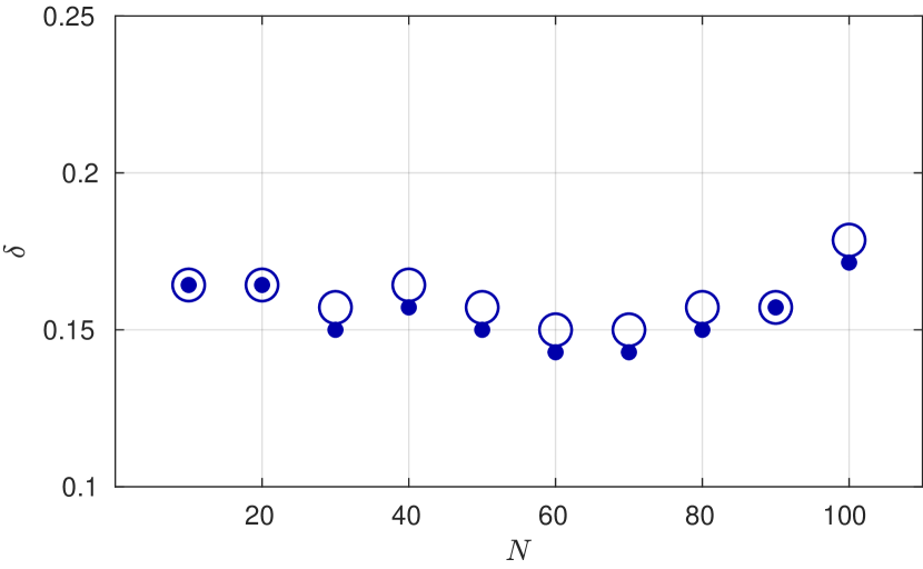
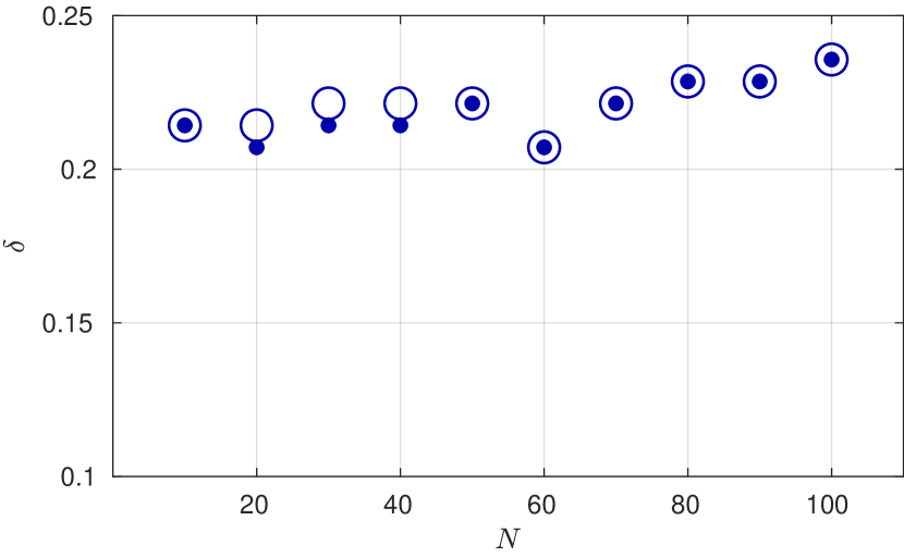
In Fig. 5.9, we plot $\delta_{\text{recon}}$ and $\delta_{\text{pred}}$ for different $N$ values for the three Reg-ROMs at both $\rm Re_{\tau}$. $\delta_{\text{recon}}$ is displayed as a smaller filled marker, while $\delta_{\text{pred}}$ is displayed as a larger empty marker. We also use different markers to distinguish the relaxation parameter, $\chi$. We note that, for a given $N$, if $(\delta,~{}\chi)_{\text{recon}}$ is also optimal for the predictive regime, the two corresponding markers of different sizes will be on top of each other.

Figs. 9(a) and 9(b) display L-ROM’s $(\delta,~{}\chi)_{\text{recon}}$ and $(\delta,~{}\chi)_{\text{pred}}$ for each $N$ for $\rm Re_{\tau}=180$ and $\rm Re_{\tau}=395$, respectively. Note that the relaxation parameter, $\chi$, is not used in L-ROM (4.1) and, therefore, is not plotted. For $\rm Re_{\tau}=180$, we find that $\delta_{\text{recon}}$ is close to but not identical to $\delta_{\text{pred}}$ for most $N$ values. For $\rm Re_{\tau}=395$, we find that $\delta_{\text{recon}}$ is identical to $\delta_{\text{pred}}$ for most $N$ values, except for $N=20,~{}30,~{}40$. In addition, for both $\rm Re_{\tau}$, we find that larger $N$ lead to larger $\delta_{\text{recon}}$ and $\delta_{\text{pred}}$.

Figs. 9(c) and 9(d) display EFR-ROM’s $(\delta,~{}\chi)_{\text{recon}}$ and $(\delta,~{}\chi)_{\text{pred}}$ for each $N$ for $\rm Re_{\tau}=180$ and $\rm Re_{\tau}=395$, respectively. For $\rm Re_{\tau}=180$, we find that $(\delta,~{}\chi)_{\text{recon}}$ is optimal for almost all $N$ values except for $N=20$. For $\rm Re_{\tau}=395$, we find that $\delta_{\text{recon}}$ is identical to $\delta_{\text{pred}}$ for all $N$ values.

In addition, we find that the EFR-ROM’s $\delta$ is less sensitive to $N$ compared to the L-ROM’s $\delta$. Moreover, for the same $\chi_{\text{recon}}$, we find that $\delta_{\text{recon}}$ and $\delta_{\text{pred}}$ are not sensitive to $\rm Re_{\tau}$. Finally, we find that $\chi=0.005$ works best for most $N$ except for $N=10,~{}20$ at $\rm Re_{\tau}=180$.

(a) L-ROM at $\rm Re_{\tau}=180$

(b) L-ROM at $\rm Re_{\tau}=395$

(c) EFR-ROM at $\rm Re_{\tau}=180$

(d) EFR-ROM at $\rm Re_{\tau}=395$

(e) TR-ROM at $\rm Re_{\tau}=180$

(f) TR-ROM at $\rm Re_{\tau}=395$

Figure 5.9: $(\delta,~{}\chi)_{\text{recon}}$ (smaller filled marker) and $(\delta,~{}\chi)_{\text{pred}}$ (larger empty marker) distributions of the three Reg-ROMs for $m=1$ and $N=10,\ldots,100$ at $\rm Re_{\tau}=180$ (left) and $\rm Re_{\tau}=395$ (right). $(\delta,~{}\chi)_{\text{recon}}$ and $(\delta,~{}\chi)_{\text{pred}}$ are the optimal filter radius and relaxation parameter values found in the reproduction and predictive regimes, respectively.

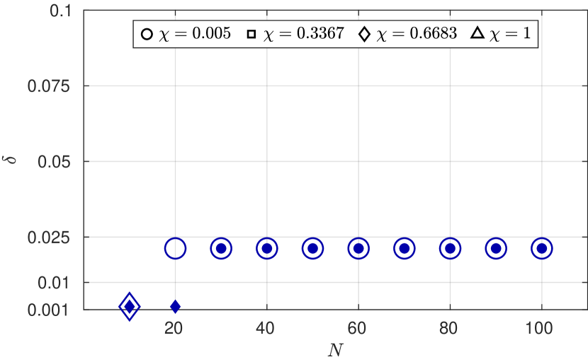
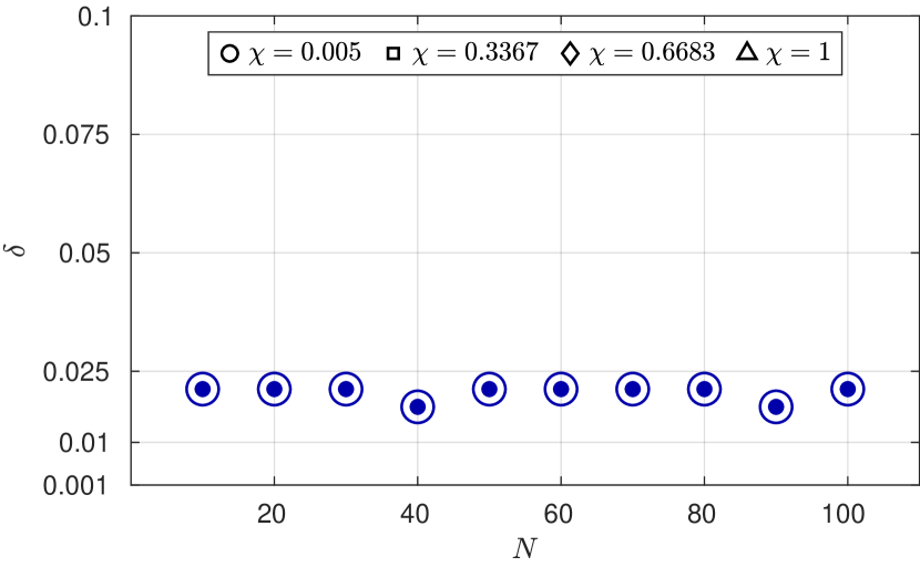
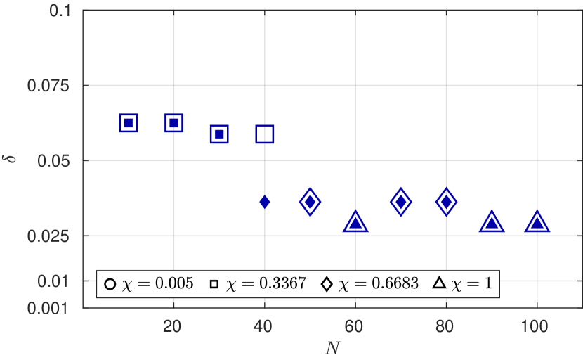
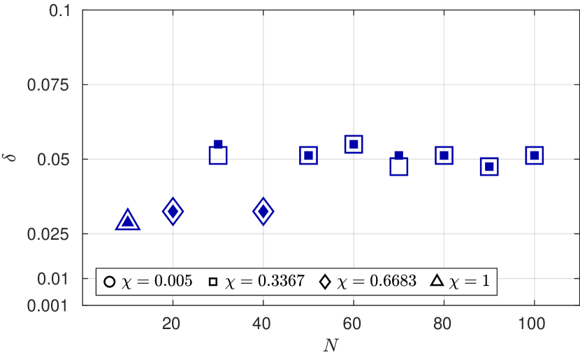
Figs. 9(e) and 9(f) display TR-ROM’s $(\delta,~{}\chi)_{\text{recon}}$ and $(\delta,~{}\chi)_{\text{pred}}$ for each $N$ for $\rm Re_{\tau}=180$ and $\rm Re_{\tau}=395$, respectively. For $\rm Re_{\tau}=180$, we find that $\delta_{\text{recon}}$ is robust for all $N$ values except for $N=40$. For $\rm Re_{\tau}=395$, we again find that $\delta_{\text{recon}}$ is robust for all $N$ values except for $N=30$ and $N=70$. Compared to the L-ROM and EFR-ROM results, we find that $(\delta,~{}\chi)_{\text{recon}}$ and $(\delta,~{}\chi)_{\text{pred}}$ are in general more sensitive to $N$ and $\rm Re_{\tau}$ in TR-ROM.

In summary, across all three Reg-ROMs with $m=1$, we find that $\delta_{\text{recon}}$ is optimal for most $N$ values for both $\rm Re_{\tau}$, demonstrating the predictive capabilities of the three Reg-ROMs and their associated parameters.

5.6.2 Reg-ROM sensitivity to the relaxation parameter $\chi$

In this section, we study the EFR-ROM and TR-ROM sensitivity to the relaxation parameter, $\chi$. To this end, we consider $\varepsilon_{u^{\prime}v^{\prime}}$ as the metric. For each $N$ and $m$, we investigate how $\varepsilon_{u^{\prime}v^{\prime}}$ is affected by $\chi$, and what $\chi$ values yield the lowest $\varepsilon_{u^{\prime}v^{\prime}}$ values.

We consider four $\chi$ values, which are uniformly sampled in the interval $[\Delta t=0.005,~{}1]$. For each $N$ and $\chi$ values, we show $\varepsilon_{u^{\prime}v^{\prime}}$ with $\delta_{\text{recon}}$ and $m=1$. We fix the filter order $m$ to be $1$ because this is the value that yields the best Reg-ROMs in the reproduction and predictive regimes (Sections 5.4.3 and 5.5.3).

(a) EFR-ROM, $\rm Re_{\tau}=180$

(b) TR-ROM, $\rm Re_{\tau}=180$

(c) EFR-ROM, $\rm Re_{\tau}=395$

(d) TR-ROM, $\rm Re_{\tau}=395$

Figure 5.10: The relative error $\varepsilon_{u^{\prime}v^{\prime}}$ (5.1) of EFR-ROM and TR-ROM with respect to $N$ and $\chi$ for $\rm Re_{\tau}=180$ (10(a) and 10(b)) and $\rm Re_{\tau}=395$ (10(c) and 10(d)) with $m=1$ and $\delta_{\text{recon}}$, where $\delta_{\text{recon}}$ is the optimal $\delta$ value found in the reproduction regime.

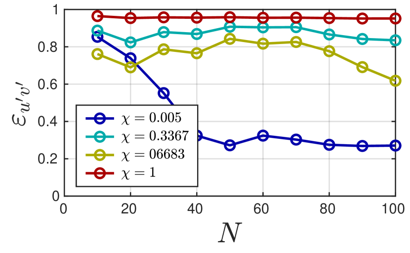
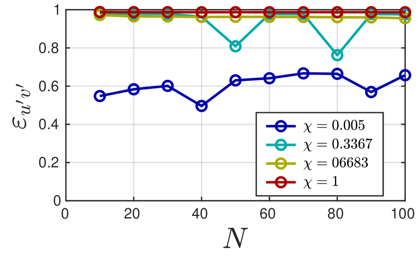
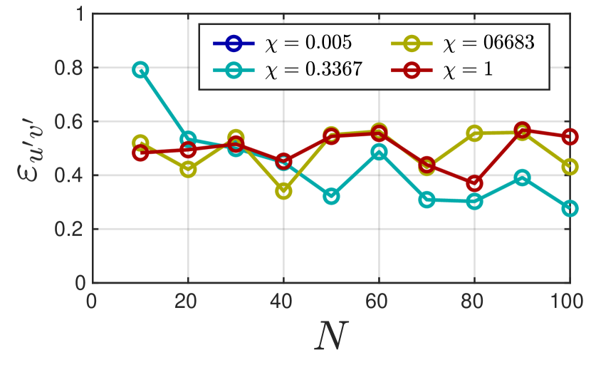
Fig. 10(a) displays the EFR-ROM results at $\rm Re_{\tau}=180$ for each $N$ and for four $\chi$ values. We recall that, in EFR-ROM (4.4), $\chi$ represents the contribution from the filtered solution at each time step. We find that EFR-ROM with $\chi=\Delta t=0.005$ yields the best results. For $\chi=1$, EFR-ROM is too dissipative and leads to an error of around $100\%$ in $\langle u^{\prime}v^{\prime}\rangle$ for all $N$ values. Although the number of samples we consider for $\chi$ is limited due to the training time, it is interesting to see that $\chi=\Delta t$ yields the best EFR-ROM results, just as in the FOM case [53, 18].

Fig. 10(b) displays the TR-ROM results for $\rm Re_{\tau}=180$ for each $N$ and for four $\chi$ values. We recall that, in TR-ROM (4.5), $\chi$ represents the amount of additional diffusion added to the G-ROM (2.3). This time, we find that TR-ROM with $\chi=\Delta t=0.005$ yields the worst results. Because the amount of diffusion added to G-ROM is not able to stabilize it, the error $\varepsilon_{u^{\prime}v^{\prime}}$ for each $N$ is more than $100\%$. For the other three $\chi$ values, for $N\leq 30$, we find that smaller $\chi$ values lead to better accuracy, and for $N\geq 40$, we find that the error $\varepsilon_{u^{\prime}v^{\prime}}$ is similar.

Fig. 10(c) displays the EFR-ROM results for $\rm Re_{\tau}=395$ for each $N$ and for four $\chi$ values. We again find that EFR-ROM with $\chi=\Delta t=0.005$ yields the best results. In contrast with the results for $\rm Re_{\tau}=180$, we find that EFR-ROM for the other three $\chi$ values leads to an error of around $100\%$ in $\langle u^{\prime}v^{\prime}\rangle$ for all $N$ values.

Fig. 10(d) displays the TR-ROM results of $\rm Re_{\tau}=395$ for each $N$ and for four $\chi$ values. Again, we find that TR-ROM for $\chi=\Delta t=0.005$ yields the worst results and the error $\varepsilon_{u^{\prime}v^{\prime}}$ is more than $100\%$ for each $N$. For $N\leq 40$, we find that $\chi=0.6683$ yields the best results for $N=20$ and $40$, and $\chi=1$ yields the best results for $N=10$ and $N=30$. For $N\geq 50$, we find that $\chi=0.3367$ yields the best results.

In summary, we found that both EFR-ROM and TR-ROM are sensitive to the relaxation parameter $\chi$. Furthermore, for EFR-ROM, we found that $\chi=\Delta t=0.005$ outperforms the other three values for almost all $N$. For TR-ROM, we found that $\chi=0.3367$ outperforms the other values for all $N$ for $\rm Re_{\tau}=180$, and for large $N$ for $\rm Re_{\tau}=395$.

5.6.3 Reg-ROM sensitivity to the filter radius $\delta$

In this section, for the optimal parameters listed in Table 1, we study the Reg-ROM sensitivity to the filter radius $\delta$ for $\rm Re_{\tau}=180$ and $\rm Re_{\tau}=395$. Our goal is to analyze the impact of $\delta$ on the Reg-ROM performance and identify the $\delta$ values that yield the best results.

(a) L-ROM, $\rm Re_{\tau}=180$

(b) L-ROM, $\rm Re_{\tau}=395$

Figure 5.11: The relative error $\varepsilon_{u^{\prime}v^{\prime}}$ (5.1) of L-ROM with respect to $\delta$ for $\rm Re_{\tau}=180$ (11(a)) and $\rm Re_{\tau}=395$ (11(b)).

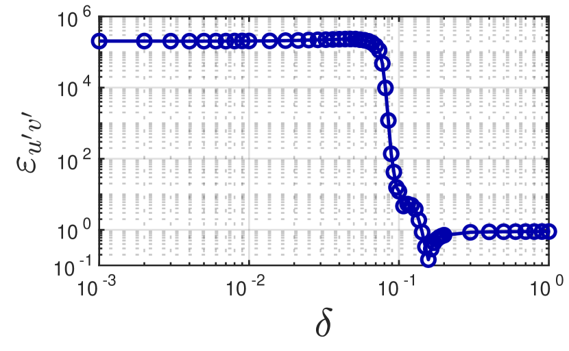
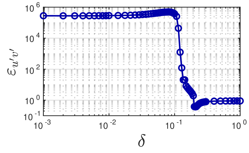
Figures 11(a) and 11(b) display the L-ROM’s $\varepsilon_{u^{\prime}v^{\prime}}$ behavior with respect to the filter radius, $\delta$, for $\rm Re_{\tau}=180$ and $\rm Re_{\tau}=395$. To discuss these results, we divide the interval $[0.001,~{}1]$ into four subintervals: (i) For $\delta\in[0.001,~{}0.01]$, $\varepsilon_{u^{\prime}v^{\prime}}$ is high and does not change with respect to $\delta$. (ii) For $\delta\in[0.01,~{}0.1]$, $\varepsilon_{u^{\prime}v^{\prime}}$ increases as $\delta$ increases, and starts decreasing when $\delta$ approaches $0.01$. In addition, a much larger error drop is observed for $\rm Re_{\tau}=180$ than for $\rm Re_{\tau}=395$. (iii) For $\delta\in[0.1,~{}0.2]$, $\varepsilon_{u^{\prime}v^{\prime}}$ decreases dramatically from $\mathcal{O}(10^{5})$ down to $0.1$ and $0.37$ for $\rm Re_{\tau}=180$ and $\rm Re_{\tau}=395$, respectively. For both $\rm Re_{\tau}$, the optimal filter radius, $\delta_{\text{recon}}$, is obtained in the interval $[0.1,~{}0.2]$. (iv) For $\delta\in[0.2,~{}1]$, $\varepsilon_{u^{\prime}v^{\prime}}$ increases as $\delta$ increases, and eventually plateaus at $\mathcal{O}(1)$ because L-ROM becomes too dissipative.

Figs. 12(a) and 12(b) display the EFR-ROM’s $\varepsilon_{u^{\prime}v^{\prime}}$ behavior with respect to the filter radius, $\delta$, for four $\chi$ values and for $\rm Re_{\tau}=180$ and $\rm Re_{\tau}=395$. From the results, we can categorize EFR-ROM’s $\varepsilon_{u^{\prime}v^{\prime}}$ behavior into two types:

(a) EFR-ROM, $\rm Re_{\tau}=180$

(b) EFR-ROM, $\rm Re_{\tau}=395$

Figure 5.12: The relative error $\varepsilon_{u^{\prime}v^{\prime}}$ (5.1) of EFR-ROM with respect to $\delta$ for $\rm Re_{\tau}=180$ (12(a)) and $\rm Re_{\tau}=395$ (12(b)).

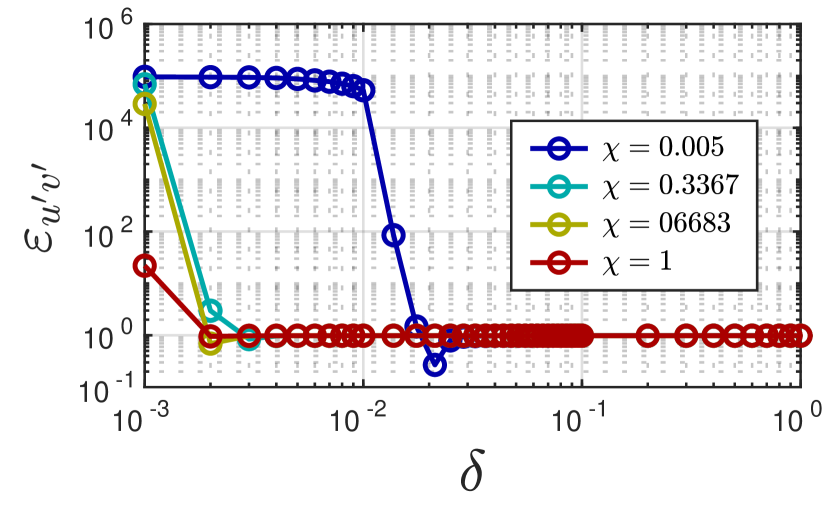
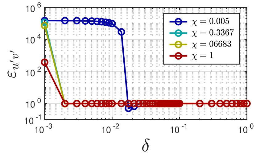
For $\chi=\Delta t=0.005$, the behavior of $\varepsilon_{u^{\prime}v^{\prime}}$ with respect to $\delta$ is similar to that for L-ROM. We can divide the interval $[0.001,~{}1]$ into three subintervals: (i) For $\delta\in[0.001,~{}0.01]$, $\varepsilon_{u^{\prime}v^{\prime}}$ decreases slightly as $\delta$ increases. (ii) For $\delta\in[0.01,~{}0.03]$, $\varepsilon_{u^{\prime}v^{\prime}}$ decreases dramatically from $\mathcal{O}(10^{5})$ down to $0.27$ and $0.5$ for $\rm Re_{\tau}=180$ and $\rm Re_{\tau}=395$, respectively. For both $\rm Re_{\tau}$ values, the optimal filter radius, $\delta_{\text{recon}}$, is obtained in the interval $[0.01,~{}0.03]$. (iii) For $\delta\in[0.03,~{}1]$, $\varepsilon_{u^{\prime}v^{\prime}}$ increases as $\delta$ increases, and eventually plateaus at $\mathcal{O}(1)$ because EFR-ROM becomes too dissipative.

For the other three $\chi$ values, we can divide the interval $[0.001,~{}1]$ into two subintervals: (i) For $\delta\in[0.001,~{}0.003]$, $\varepsilon_{u^{\prime}v^{\prime}}$ decreases dramatically to $\mathcal{O}(1)$. However, the fact that there is no $\delta$ such that $\varepsilon_{u^{\prime}v^{\prime}}$ is below $1$ suggests that the optimal filter radius $\delta_{\text{recon}}$ is either very sensitive, which requires more sampling points in the interval $[0.001,~{}0.003]$, or it does not exist at all. (ii) For $\delta\in[0.003,~{}1]$, $\varepsilon_{u^{\prime}v^{\prime}}$ is mostly $\mathcal{O}(1)$, suggesting that, for these $\chi$ values, EFR-ROM is too dissipative regardless of the $\delta$ value.

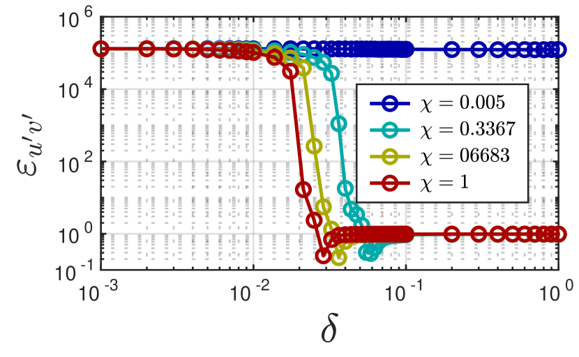
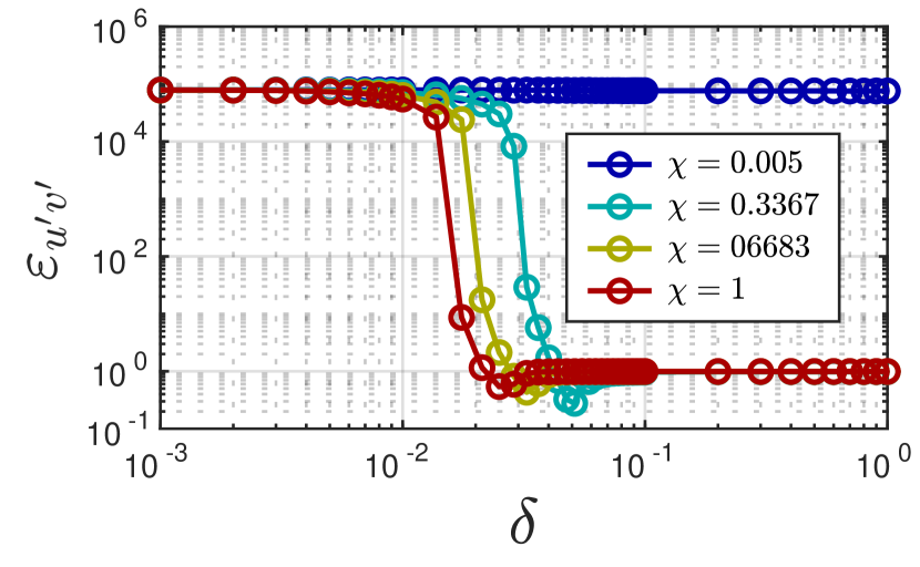
Figs. 13(a) and 13(b) display the TR-ROM’s $\varepsilon_{u^{\prime}v^{\prime}}$ behavior with respect to the filter radius, $\delta$, for four $\chi$ values and for $\rm Re_{\tau}=180$ and $\rm Re_{\tau}=395$.

(a) TR-ROM, $\rm Re_{\tau}=180$

(b) TR-ROM, $\rm Re_{\tau}=395$

Figure 5.13: The relative error $\varepsilon_{u^{\prime}v^{\prime}}$ (5.1) of TR-ROM with respect to $\delta$ for $\rm Re_{\tau}=180$ (13(a)) and $\rm Re_{\tau}=395$ (13(b)).

From the results, we can categorize TR-ROM’s $\varepsilon_{u^{\prime}v^{\prime}}$ behavior into two types:

For $\chi=\Delta t=0.005$, there is no improvement in $\varepsilon_{u^{\prime}v^{\prime}}$ as $\delta$ increases. This suggests that $\chi$ is so small that, regardless of how large the dissipative term $({\bm{u}}_{r}-\overline{{\bm{u}}}_{r})$ (4.6) (determined by $\delta$) is, the total contribution $\chi({\bm{u}}_{r}-\overline{{\bm{u}}}_{r})$ is too small to stabilize G-ROM (2.3).

For the other three $\chi$ values, the TR-ROM’s behavior of $\varepsilon_{u^{\prime}v^{\prime}}$ with respect to $\delta$ is similar to that of L-ROM and EFR-ROM for $\chi=0.005$. We can divide the interval $[0.001,~{}1]$ into three subintervals: (i) For $\delta\in[0.001,~{}0.01]$, $\varepsilon_{u^{\prime}v^{\prime}}$ decreases slightly as $\delta$ increases. (ii) For $\delta\in[0.01,~{}0.1]$, $\varepsilon_{u^{\prime}v^{\prime}}$ decreases dramatically from $\mathcal{O}(10^{5})$ down to its optimal value. Furthermore, the smaller the $\chi$ value, the larger the $\delta$ value required to achieve its optimal $\varepsilon_{u^{\prime}v^{\prime}}$. This is expected because assuming that the total contribution $\chi({\bm{u}}_{r}-\overline{{\bm{u}}}_{r})$ for optimal TR-ROM is fixed, larger $\chi$ will then require smaller $\delta$. (iii) For $\delta\in[0.1,~{}1]$, $\varepsilon_{u^{\prime}v^{\prime}}$ increases as $\delta$ increases, and eventually plateaus at $\mathcal{O}(1)$ because TR-ROM becomes too dissipative.

In summary, we find that all three Reg-ROMs are sensitive to the filter radius, $\delta$. For EFR-ROM and TR-ROM, $\delta_{\text{recon}}$ is affected by the relaxation parameter $\chi$, and in the worst-case scenario, $\delta_{\text{recon}}$ might not even exist. In addition, we find that the optimal range for $\delta$ and the effect of $\chi$ are similar for the two $\rm Re_{\tau}$ values.

6 Conclusions and Future Work

In this paper, we propose the time-relaxation ROM (TR-ROM), which is a novel regularized ROM (Reg-ROM) for under-resolved turbulent flows. The TR-ROM employs ROM spatial filtering to smooth out the flow velocity and eliminate the spurious numerical oscillations displayed by the standard Galerkin ROM (G-ROM) (i.e., the ROM that does not use any numerical stabilization). We emphasize that one novel feature of the TR-ROM, which distinguishes it from the other Reg-ROM in current use (i.e., the Leray ROM (L-ROM) and the evolve-filter-relax ROM (EFR-ROM)), is that it introduces different dissipation for the large resolved scales and the small resolved scales. This is in stark contrast with the other two types of Reg-ROMs, i.e, L-ROM and EFR-ROM, which use spatial filtering without distinguishing between small and large resolved scales.

To assess the new TR-ROM, we compare it with the L-ROM and the EFR-ROM in the numerical simulation of the turbulent channel flow at $Re_{\tau}=180$ and $Re_{\tau}=395$ in both the reproduction and the predictive regimes. The spatial filtering in all three Reg-ROMs is performed using the first-order ROM differential filter or the higher-order ROM algebraic filter. We also investigate the sensitivity of the Reg-ROMs with respect to the following parameters: the time interval, the relaxation parameter, and the filter radius. To our knowledge, this is the first numerical comparison of different Reg-ROMs in the numerical simulation of turbulent flows.

Our numerical investigation yields the following conclusions: All three Reg-ROMs are dramatically more accurate than the classical G-ROM without significantly increasing its computational cost. In fact, with respect to several second-order turbulence statistics, the three Reg-ROMs’ errors are much lower than the projection error. In addition, with the optimal parameters, the new TR-ROM yields more accurate results than the L-ROM and the EFR-ROM in all tests. Our numerical investigation also shows that the HOAF with filter order $m=1$ yields the best results for most of the $N$ values. On the other hand, the HOAF with $m>1$ works better for small $N$, i.e., $N\leq 20$, at lower Reynolds number $\rm Re_{\tau}=180$.

The sensitivity study shows that the optimal parameters trained in the reproduction regime $(\delta,~{}\chi)_{\text{recon}}$ are also optimal in the predictive regime for most of the $N$ values and for all three Reg-ROMs. Although all three Reg-ROMs are sensitive with respect to the relaxation parameter, $\chi$, and filter radius, $\delta$, the optimal range for $\delta$ and the effect of $\chi$ are similar for the two $\rm Re_{\tau}$ values.

From the numerical investigation of the HOAF (Section A.2.3), we found that the HOAF in the POD setting is indeed a spatial filter, and has a similar behavior as in the SEM setting, i.e., the higher-order filter (larger $m$) tends to damp the higher index modes more, and has less impact on the lower index modes.

The first steps in the numerical investigation of the new TR-ROM for the turbulent channel flow have been encouraging. There are, however, several other research directions that should be pursued next. For example, one can investigate whether ROM approximate deconvolution [56, 57] can be leveraged to further increase the localization of the dissipation mechanism in the new TR-ROM. One could also compare the approximate deconvolution approach with the effect of increasing the order of the higher-order algebraic filter (3.3) in TR-ROM. Finally, TR-ROM’s numerical analysis, which could yield new, robust parameter scalings [58], should be performed.

7 Acknowledgments

This research used the Delta advanced computing and data resource which is supported by the National Science Foundation (award OAC 2005572) and the State of Illinois. The third author gratefully acknowledges NSF funding support through grant DMS-2012253.

Appendix A HOAF Investigation

In this section, we perform a theoretical and numerical investigation of the HOAF (3.3), which, for clarity, we rewrite below:

Given ${\bm{u}}_{\text{r}}=\sum_{j=1}^{N}u_{\text{r},j}\bm{\varphi}_{j}$, find $\overline{{\bm{u}}}_{\text{r}}=\sum_{j=1}^{N}\overline{u}_{\text{r},j}\bm{\varphi}_{j}$ such that

$$\left(\mathbbm{I}+\delta^{2m}A^{m}\right)\underline{\overline{u}}_{\text{r}}={\underline{u}}_{\text{r}},$$ (A.1)

where ${\underline{u}}_{\text{r}}$ and $\underline{\overline{u}}_{\text{r}}$ are the vectors of ROM basis coefficients of ${\bm{u}}_{\text{r}}$ and $\overline{{\bm{u}}}_{\text{r}}$, respectively, and $m\geq 2$ is an integer.

We note that we consider only integers $m\geq 2$ because, as explained in Remark 3.1, the standard (low-order) DF (3.2) can be considered as a particular case of HOAF with $m=1$. Thus, to distinguish between the DF and the HOAF, in this section we exclusively consider $m\geq 2$ in HOAF.

In addition, we note that the expansions for ${\bm{u}}_{\text{r}}$ and $\overline{{\bm{u}}}_{\text{r}}$ do not include the time-averaged velocity field, $\bm{\varphi}_{0}$. This is in contrast with the expansion (2.2), which does include $\bm{\varphi}_{0}$. The reason for not including $\bm{\varphi}_{0}$ in our expansions is that, in our numerical investigation, we decided not to filter the time-averaged velocity field, $\bm{\varphi}_{0}$, because this strategy was shown in [16] to yield more accurate results.

Moreover, we note that, in a spectral element setting, in [32] it was shown that HOAF (A.1) is a spatial filter that attenuates the high wavenumber components of the input field. Furthermore, it was also shown that the exponent $m$ in the HOAF (A.1) controls the percentage of filtering at different wavenumbers: As $m$ increases, the amount of filtering increases for the high wavenumber components of the input field, and decreases for the low wavenumber components [32, Figure 1].

In this section, we investigate whether the HOAF (A.1) is a spatial filter. We also study the role of the exponent $m$ in the HOAF (A.1). We address this question first from a theoretical point of view (Section A.1), and then from a computational point of view (Section A.2).

A.1 Theoretical Investigation

In this section, we perform a theoretical investigation of HOAF (A.1). To this end, we first discuss the weak form (variational formulation) of HOAF, which is needed to construct the ROM discretization of HOAF.

We note that the weak form for DF is clear: The DF linear systems (3.2) results from the ROM discretization of the weak form of the Helmholtz equation (3.1). Thus, because the DF can be interpreted as the HOAF (A.1) with $m=1$, we hope we can leverage that to find the HOAF weak form.

We emphasize that finding the HOAF weak form is important. Indeed, the connection between HOAF (A.1) and its conjectured weak form is used in the physical interpretation of the time relaxation term (Case 2 in Section 4.3). More importantly, the HOAF weak form can tell us whether HOAF is a spatial filter, just as in the DF case.

In this section, we discuss the HOAF weak form for $m=2$. We believe this discussion can be naturally extended to higher $m$ values.

To discuss the HOAF weak form and the associated ROM formulation, we formally extend the mixed finite element discretization of the biharmonic equation proposed by Falk and Osborn [59], which is based on earlier work by Ciarlet and Raviart [60], Glowinski [61], and Mercier [62].

Because DF is HOAF with $m=1$, it is natural to associate the following PDE with HOAF: Given ${\bm{u}}\in L^{2}(\Omega)$, find $\overline{{\bm{u}}}\in H_{0}^{2}(\Omega)$ such that

$$\delta^{4}\Delta^{2}\overline{{\bm{u}}}+\overline{{\bm{u}}}={\bm{u}}\qquad\text{in }\Omega,$$ (A.2)

$$\overline{{\bm{u}}}=\frac{\partial\overline{{\bm{u}}}}{\partial{\bf n}}=0\qquad\quad\text{on }\partial\Omega.$$ (A.3)

We note that, as pointed out in [60], the most straightforward finite element discretization of the biharmonic equation is to use a conforming method, in which the finite element space is a subspace of $H_{0}^{2}(\Omega)=\{{\bf v}\in H^{2}(\Omega):{\bf v}=\frac{\partial{\bf v}}{\partial{\bm{n}}}={\bm{0}}~{}\text{on}~{}\partial\Omega\}$. Constructing such subspaces, however, requires sophisticated finite elements. Thus, to avoid these computational challenges, noncoforming finite elements have been proposed, in which the finite element space are subspaces of $H^{1}(\Omega)$. One such strategy is the mixed finite element formulation of the biharmonic equation proposed in [59], which utilizes standard finite element spaces in $H^{1}(\Omega)$.

We emphasize that, in our numerical investigation in Section 5, the spectral element discretization used to construct the ROM basis function is posed in $H_{0}^{1}(\Omega)$. Thus, we extend the mixed finite element strategy proposed in [59] to our ROM setting. To this end, we first define the following auxiliary variable:

$${\bf w}:=-\Delta\overline{{\bm{u}}}.$$ (A.4)

Next, we extend the weak form $(3.3)$ in [59] to the PDE we considered in (A.2)–(A.3): Given ${\bm{u}}\in L^{2}(\Omega)$, find $({\bf w},\overline{{\bm{u}}})\in(H_{0}^{1}(\Omega),H_{0}^{1}(\Omega))$ such that

$$({\bf w},{\bf v}_{{\bf w}})-(\nabla\overline{{\bm{u}}},\nabla{\bf v}_{{\bf w}})=0\qquad\qquad\quad\forall\,{\bf v}_{{\bf w}}\in H_{0}^{1}(\Omega)$$ (A.5)

$$\delta^{4}\,(\nabla{\bf w},\nabla{\bf v}_{\overline{{\bm{u}}}})+(\overline{{\bm{u}}},{\bf v}_{\overline{{\bm{u}}}})=({\bm{u}},{\bf v}_{\overline{{\bm{u}}}})\qquad\forall\,{\bf v}_{\overline{{\bm{u}}}}\in H_{0}^{1}(\Omega)$$ (A.6)

Remark A.1 (ROM-FEM Weak Form).

We note that, although the weak form (A.5)–(A.6) is similar to the weak form $(3.3)$ in [59], there are several significant differences. Probably the most important difference is that we use $H_{0}^{1}(\Omega)$ instead of $H^{1}(\Omega)$ to approximate the auxiliary variable ${\bf w}$. Our choice is motivated by the spectral element space used in our numerical investigation in Section 5, which is a subspace of $H_{0}^{1}(\Omega)$.

To find the ROM discretization of the weak formulations (A.5) and (A.6), we use the classical Galerkin method: For (A.5), we consider the ROM expansions $\overline{{\bm{u}}}\approx\overline{{\bm{u}}}_{\text{r}}=\sum_{j=1}^{N}\overline{u}_{\text{r},j}\bm{\varphi}_{j}$ and ${\bf w}\approx{\bf w}_{\text{r}}=\sum_{j=1}^{N}w_{\text{r},j}\bm{\varphi}_{j}$, and choose the test functions ${\bf v}_{{\bf w}}:=\bm{\varphi}_{i},i=1,\ldots,N$. This yields the following linear system:

$$\mathbbm{I}\underline{w}_{\text{r}}=A\underline{\overline{u}}_{\text{r}},$$ (A.7)

where $\underline{w}_{\text{r}}$ and $\underline{\overline{u}}_{\text{r}}$ are the vector of ROM coefficients of ${\bf w}_{\text{r}}$ and $\overline{{\bm{u}}}_{\text{r}}$, respectively, and $\mathbbm{I}$ and $A$ are the identity and ROM stiffness matrices, respectively.

To find the ROM discretization of the weak formulation (A.6), we use again the ROM expansions $\overline{{\bm{u}}}\approx\overline{{\bm{u}}}_{\text{r}}=\sum_{j=1}^{N}\overline{u}_{\text{r},j}\bm{\varphi}_{j}$ and ${\bf w}\approx{\bf w}_{\text{r}}=\sum_{j=1}^{N}w_{\text{r},j}\bm{\varphi}_{j}$, and choose the test functions ${\bf v}_{\overline{{\bm{u}}}}:=\bm{\varphi}_{i},i=1,\ldots,N$. This yields the following linear system:

$$\delta^{4}A\underline{w}_{\text{r}}+\mathbbm{I}\underline{\overline{u}}_{\text{r}}=\mathbbm{I}\underline{u}_{\text{r}},$$ (A.8)

where $\underline{u}_{\text{r}}$ is the vector of ROM coefficients of ${\bm{u}}_{\text{r}}$. Plugging the formula for $\underline{w}_{\text{r}}$ in (A.7) in (A.8) yields

$$\delta^{4}A\left(A\underline{\overline{u}}_{\text{r}}\right)+\mathbbm{I}\underline{\overline{u}}_{\text{r}}=\mathbbm{I}\underline{u}_{\text{r}},$$ (A.9)

which is exactly the HOAF linear system (A.1) for $m=2$.

Thus, for $m=2$, we have shown that the ROM discretization of the weak forms (A.5) and (A.6) is the HOAF linear system (A.1).

We note that, in a spectral element setting, the PDE associated with HOAF (A.1) was discussed in [32] (albeit with a missing minus sign).

A.2 Numerical Investigation

In this section, we investigate whether the HOAF (A.1) is a spatial filter by solving (A.1) and examining if the output $\overline{{\bm{u}}}$ is smoother compared to the input ${\bm{u}}$. We also study the role of the exponent $m$ in the HOAF. In sections A.2.1–A.2.2, we investigate the HOAF in one- and two-dimensional spectral element (SEM) settings. In section A.2.3, we investigate the HOAF in a POD setting. We note that a similar numerical investigation was carried out in the spectral element setting in [32], where it was shown that HOAF (A.1) is a low-pass filter [32, Figure 1].

A.2.1 One-Dimensional SEM Setting

We consider the spatial domain $\Omega=[0,1]$ and construct the HOAF (A.1) using a SEM discretization that consists of a $64$-dimensional array of $7$th-order spectral elements. Note that, in the SEM setting, instead of $A^{m}$ we use $(B^{-1}A)^{m}$ in (A.1), and ${\underline{u}}$ and ${\underline{\overline{u}}}$ are the SEM basis coefficients for the input (unfiltered) and output (filtered) functions, respectively.

We construct an input function $u$ that has both low and high wavenumber components:

$$u(x)=0.5\sin(2\pi x)+0.5\sin(10\pi x)+2\sin(20\pi x),$$ (A.10)

and set the filter radius $\delta$ to be $0.025$. We then consider four $m$ values and compare the corresponding HOAF output $\overline{u}$ with the input function $u$ in Fig. A.1.

Figure A.1: Comparison of the input function $u(x)=0.5\sin(2\pi x)+0.5\sin(10\pi x)$ $+2\sin(20\pi x)$ and four HOAF outputs $\overline{u}$ that correspond to $m=1,~{}2,~{}3,~{}4$, and $\delta=0.025$.

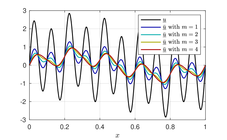
The $m=1$ results show that, although HOAF has attenuated the high wavenumber ($k=20$) component of the input function, that component is still visible. However, as we increase the HOAF order (i.e., use $m=2,3,4$), the high wavenumber component of the input function starts to significantly decrease. In fact, for $m=4$, the high wavenumber component is practically eliminated. We also note that the medium wavenumber ($k=10$) component of the input function is affected differently by the different $m$ values: For $m=1$, the medium wavenumber component is slightly attenuated. In contrast, for $m=4$, the medium wavenumber component remains unchanged. Finally, the low wavenumber ($k=2$) component of the input function is practically unaffected by the HOAF order. Thus, the results in Fig. A.1 suggest that, as expected, using the classical DF (i.e., HOAF with $m=1$) attenuates the medium and high wavenumber components of the input function. The higher-order HOAF (i.e., HOAF with $m=2,3,4$) attenuates more the high wavenumber component, and almost not at all the medium wavenumber component.

A.2.2 Two-Dimensional SEM Setting

We consider the spatial domain $\Omega=[0,1]^{2}$ and construct the HOAF (A.1) using a SEM discretization that consists of a $12\times 12$ array of $7$th-order spectral elements. We construct an input function $u$ that has both low and high wavenumber components:

$$u(x,y)=0.5\sin(2\pi x)\sin(2\pi y)+\sin(4\pi x)\sin(4\pi y)+2\sin(6\pi x)\sin(6\pi y),$$ (A.11)

and set the filter radius $\delta$ to be $0.06$. We then consider three $m$ values and compare the corresponding HOAF output $\overline{u}$ with the input function $u$ in Fig. A.2.

(a) Input function $u$

(b) $\overline{u}$ with $m=1$

(c) $\overline{u}$ with $m=2$

(d) $\overline{u}$ with $m=3$

Figure A.2: Comparison of the input function $u(x,y)=0.5\sin(2\pi x)\sin(2\pi y)+\sin(4\pi x)\sin(4\pi y)+2\sin(6\pi x)\sin(6\pi y)$ and three HOAF outputs $\overline{u}$ corresponding to $m=1,~{}2,~{}3$ with $\delta=0.06$.

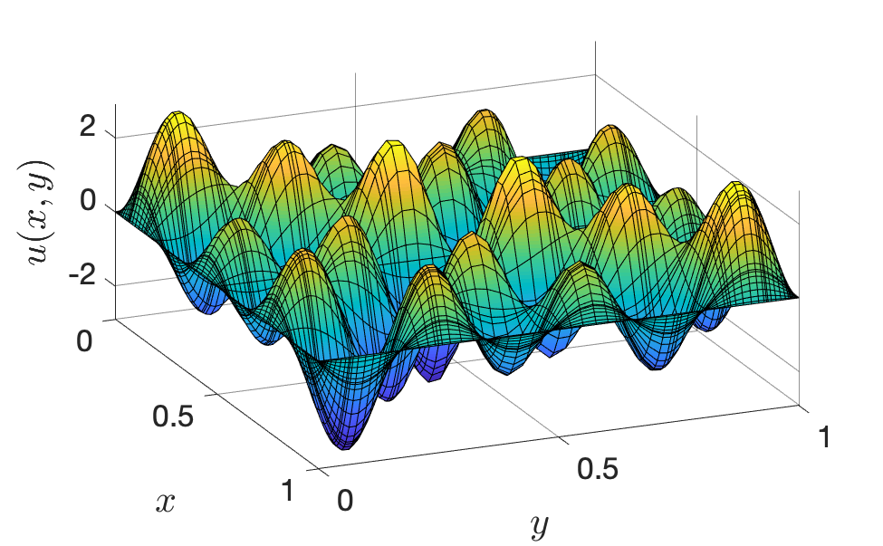
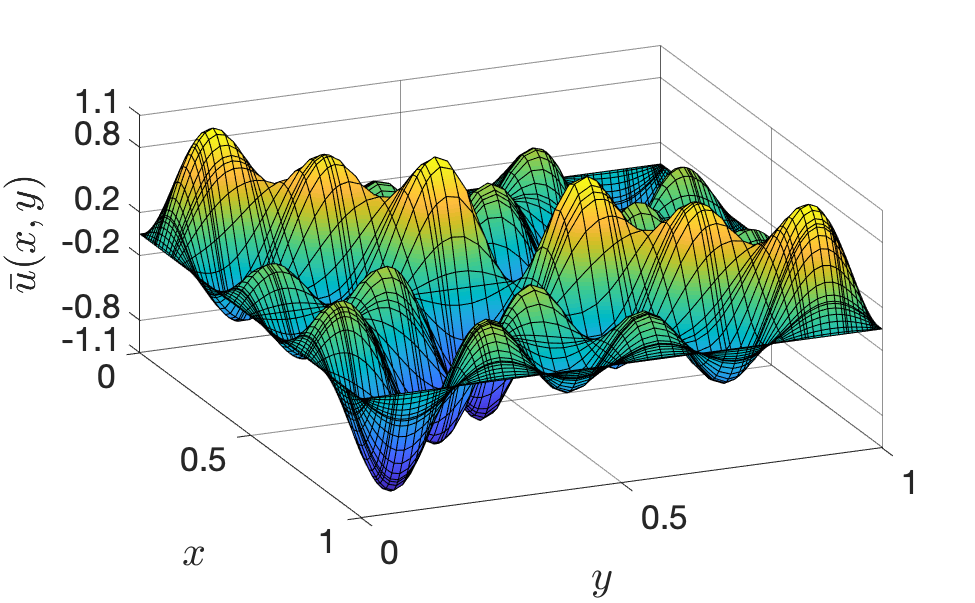
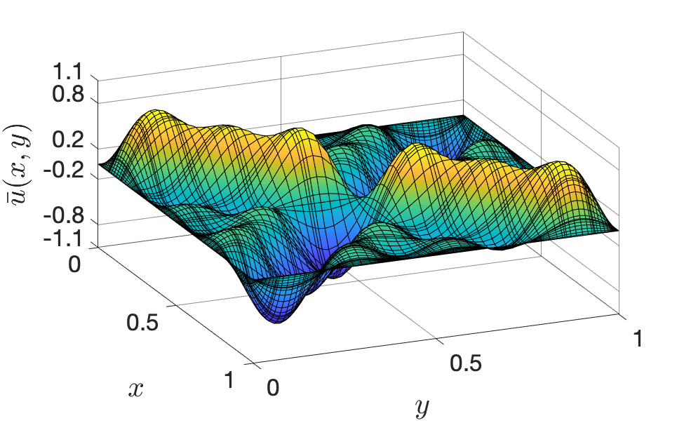
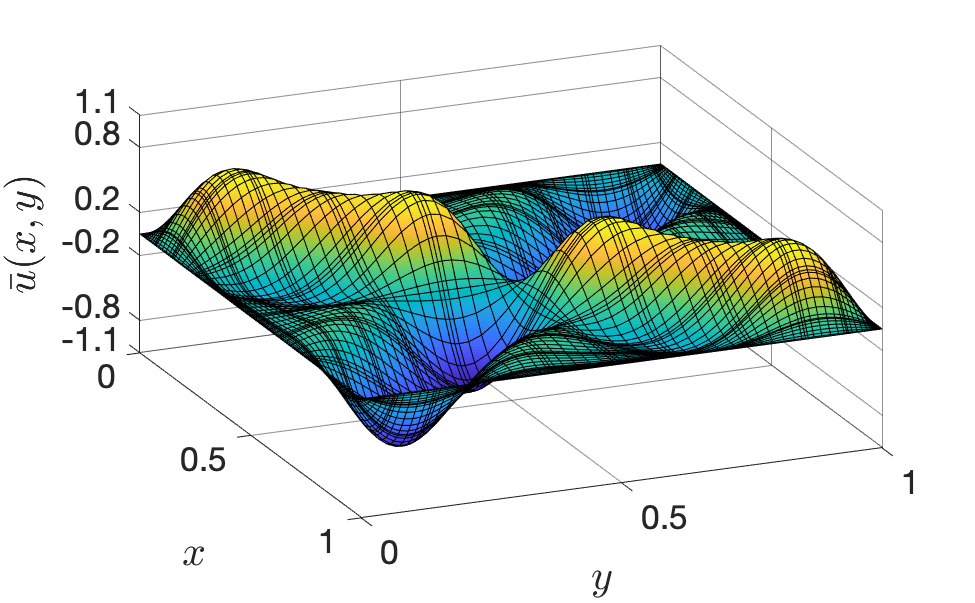
The $m=1$ results show that, although HOAF has attenuated the high wavenumber ($(k_{1},k_{2})=(6,6)$ component of the input function, that component is still visible. However, as we increase the HOAF order (i.e., use $m=2,3$), the high wavenumber component of the input function starts to significantly decrease. We also note that the medium wavenumber ($(k_{1},k_{2})=(4,4)$) component of the input function is affected differently by the different $m$ values: For $m=1$, the medium wavenumber component is slightly attenuated. In contrast, for $m=3$, the medium wavenumber component remains unchanged. Finally, the low wavenumber ($(k_{1},k_{2})=(2,2)$) component of the input function is unaffected by the HOAF order. Thus, the results in Fig. A.2 again suggest that the classical DF (i.e., HOAF with $m=1$) attenuates the medium and high wavenumber components of the input function. The higher-order HOAF (i.e., HOAF with $m=2,3$) attenuates more the high wavenumber component, and almost not at all the medium wavenumber component.

A.2.3 POD Setting

We investigate the HOAF (A.1) in a POD setting. In particular, we consider the POD basis functions for the turbulent channel flow at $\rm Re_{\tau}=180$, as detailed in Section 5.2. The HOAF is constructed using $N=100$ $L^{2}$ POD basis functions, and filter radius $\delta=0.08125$. The $\delta$ value is chosen such that the damping is neither too strong nor too weak.

To understand how each POD basis function is affected by the HOAF with different $m$ values, we consider the following procedure: For a given $m$ value, and for each mode $i$, where $1\leq i\leq N$, we construct an input coefficient vector ${\underline{u}}=[0,\ldots,0,1,0,\ldots,0]^{T}$, where $1$ appears only in the $i$th component (i.e., $u_{i}=1$) and obtain the output vector ${\underline{\overline{u}}}$ by solving the HOAF linear system (A.1.) The $i$th component of the output vector ${\underline{\overline{u}}}$ (i.e., $\overline{u}_{i}$) indicates the amount of damping caused by the HOAF in the $i$th POD basis function.

Fig. A.3 displays the unfiltered and the filtered coefficient magnitude of the $i$th POD basis function, $u_{i}$ (black) and $\overline{u}_{i}$ (multi-colored), with four filter order values $m=1,~{}2,~{}3,~{}4$, for $i=1,\ldots,N$.

Figure A.3: The unfiltered and filtered coefficient magnitude of the $i$th POD basis function, $u_{i}$ and $\overline{u}_{i}$, with four filter order values $m=1,~{}2,~{}3,~{}4$ for $i=1,\ldots,N$. The HOAF (A.1) is formed using $N=100$ $L^{2}$ POD basis functions and a filter radius of $\delta=0.08125$.

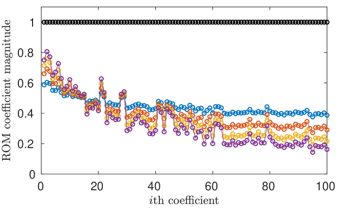
Note that, for each mode $i$, although the input vector ${\underline{u}}$ has only zero components except the $i$th component (i.e., $u_{i}=1$), the output vector ${\underline{\overline{u}}}$ could have a nonzero $j$th component (i.e., $\overline{u}_{j}\neq 0$) for $j\neq i$, because the input vector ${\underline{u}}$ is not necessary an eigenvector of the HOAF. In Fig. A.3, for each mode $i$, we show only the behavior of $\overline{u}_{i}$ because the purpose of this study is to investigate how each $i$th POD basis function is affected by the HOAF. In addition, we observe that, although ${\underline{\overline{u}}}$ contains excitations of other modes, these nonzero values are relatively small compared to the $i$th component.

In Fig. A.3, we see the expected behavior: Increasing $m$ yields a sharper drop in the transfer function (${\bar{u}}_{i}/{u_{i}}$) for high mode numbers, $i$, with less suppression of the low mode numbers, which is consistent with an interpretation of the POD modes as “Fourier” modes. Note that all the curves intersect at ${\bar{u}}_{i}/{u_{i}}\approx 1/2$ near $i=15$, which implies that modes with $i<15$ have characteristic length scales $\lambda_{i}>\delta=0.08125$, given that we expect

$$\frac{{\bar{u}}_{i}}{u_{i}} \sim \frac{1}{1+(\delta/\lambda_{i})^{2m}}\;.$$

Thus, we see that, in this case, the HOAF provides a convenient means to associate a length scale with each mode.

Figs. A.4–A.6 illustrate the physical-space effect of the HOAF with $m=1,~{}2,~{}3,~{}4$ and $\delta=0.08125$ for modes $i=1,15$, and $100$. It is clear that the higher-order filter (i.e., a larger $m$ value) has less damping in mode $i=1$ and more damping in mode $i=100$. For mode $i=15$, all $m$ values yield similar damping. Because the filtered basis function is simply the unfiltered basis function weighted by the coefficients given in Fig. A.3, we expect the filtered basis function for different $m$ values to differ only in the magnitude. Thus, in Figs. A.4–A.6, to compare the damping for different $m$ values, we compare the maximum and minimum magnitudes that are reported in the legends.

Figure A.4: Comparison of streamwise component of the 1st filtered POD basis function for four filter order values $m=1,~{}2,~{}3,~{}4$. The HOAF is constructed with $N=100$ basis functions and filter radius $\delta=0.08125$. The display range is fixed to be $[-0.4343,~{}0.3514]$ and the maximum and minimum magnitudes are reported in the legend.

Figure A.5: Comparison of streamwise component of the 15th filtered POD basis function for four filter order values $m=1,~{}2,~{}3,~{}4$. The HOAF is constructed with $N=100$ basis functions and filter radius $\delta=0.08125$. The display range is fixed to be $[-0.3254,~{}0.3020]$ and the maximum and minimum magnitudes are reported in the legend.

Figure A.6: Comparison of streamwise component of the 100th filtered POD basis function for four filter order values $m=1,~{}2,~{}3,~{}4$. The HOAF is constructed with $N=100$ basis functions and filter radius $\delta=0.08125$. The display range is fixed to be $[-0.2201,~{}0.2201]$ and the maximum and minimum magnitudes are reported in the legend.

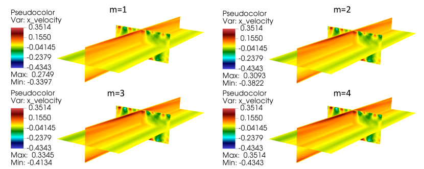
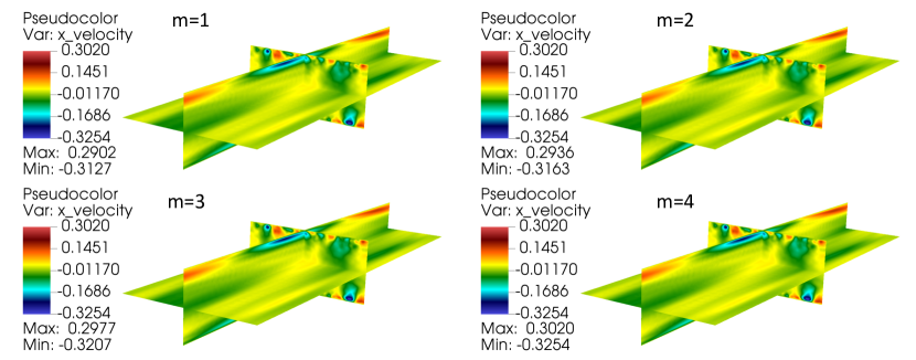
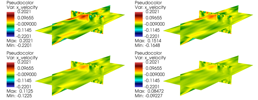
Overall, these results show that the HOAF in the POD setting has a similar behavior as in the SEM setting, that is, larger $m$ values tend to damp the higher modes more and have less impact on the lower modes compared to smaller $m$ values. However, unlike in the SEM setting where the low-wave number modes are usually undamped regardless of the $m$ value, all POD modes are damped in the POD setting.

In this numerical investigation we exclusively used $L^{2}$ POD basis functions, which is the most popular choice in reduced order modeling. We note, however, that the $H^{1}_{0}$ POD basis functions could provide a clearer illustration of the HOAF spatial filtering capabilities. Indeed, as highlighted in [14], the $H^{1}_{0}$ POD basis functions are better in capturing the small-scale structures and distinguishing them from the large-scale structures in the solution compared to the $L^{2}$ POD basis functions. Hence, we anticipate more distinct results in the filtered coefficients when the HOAF is constructed by using the $H^{1}_{0}$ POD basis functions.

References

- [1] S. L. Brunton and J. N. Kutz. Data-Driven Science and Engineering: Machine Learning, Dynamical Systems, and Control. Cambridge University Press, 2019.
- [2] J. S. Hesthaven, G. Rozza, and B. Stamm. Certified Reduced Basis Methods for Parametrized Partial Differential Equations. Springer, 2015.
- [3] B. R. Noack, M. Morzynski, and G. Tadmor. Reduced-Order Modelling for Flow Control, volume 528. Springer Verlag, 2011.
- [4] A. Quarteroni, A. Manzoni, and F. Negri. Reduced Basis Methods for Partial Differential Equations: An Introduction, volume 92. Springer, 2015.
- [5] J. Kim, P. Moin, and R. Moser. Turbulence statistics in fully developed channel flow at low Reynolds number. J. Fluid Mech., 177:133–166, 1987.
- [6] R.D. Moser, J. Kim, and N. N. Mansour. Direct numerical simulation of turbulent channel flow up to = 590. Phys. Fluids, 11(4):943–945, 1999.
- [7] S. E. Ahmed, S. Pawar, O. San, A. Rasheed, T. Iliescu, and B. R. Noack. On closures for reduced order models A spectrum of first-principle to machine-learned avenues. Phys. Fluids, 33(9):091301, 2021.
- [8] P.T. Tsai, P. Fischer, and E. Solomonik. Accelerating the Galerkin reduced-order model with the tensor decomposition for turbulent flows. arXiv preprint arXiv:2311.03694, 2023.
- [9] M. Couplet, P. Sagaut, and C. Basdevant. Intermodal energy transfers in a proper orthogonal decomposition–Galerkin representation of a turbulent separated flow. J. Fluid Mech., 491:275–284, 2003.
- [10] K. Carlberg, C. Bou-Mosleh, and C. Farhat. Efficient non-linear model reduction via a least-squares Petrov–Galerkin projection and compressive tensor approximations. Int. J. Num. Meth. Eng., 86(2):155–181, 2011.
- [11] E. J. Parish, C. Wentland, and K. Duraisamy. The adjoint Petrov–Galerkin method for non-linear model reduction. Comput. Meth. Appl. Mech. Eng., 365:112991, 2020.
- [12] C. Mou, E. Merzari, O. San, and T. Iliescu. An energy-based lengthscale for reduced order models of turbulent flows. Nucl. Eng. Des., 412:112454, 2023.
- [13] K. Kaneko. An augmented basis method for reduced order models of turbulent flow. PhD thesis, 2022.
- [14] L. Fick, Y. Maday, A. T. Patera, and T. Taddei. A stabilized POD model for turbulent flows over a range of Reynolds numbers: Optimal parameter sampling and constrained projection. J. Comp. Phys., 371:214–243, 2018.
- [15] P.S. Johansson, H.I. Andersson, and E.M. Rønquist. Reduced-basis modeling of turbulent plane channel flow. Comput. & Fluids, 35(2):189–207, 2006.
- [16] D. Wells, Z. Wang, X. Xie, and T. Iliescu. An evolve-then-filter regularized reduced order model for convection-dominated flows. Int. J. Num. Meth. Fluids, 84:598––615, 2017.
- [17] F. Sabetghadam and A. Jafarpour. regularization of the POD-Galerkin dynamical systems of the Kuramoto–Sivashinsky equation. Appl. Math. Comput., 218(10):6012–6026, 2012.
- [18] M. Strazzullo, M. Girfoglio, F. Ballarin, T. Iliescu, and G. Rozza. Consistency of the full and reduced order models for evolve-filter-relax regularization of convection-dominated, marginally-resolved flows. Int. J. Num. Meth. Eng., 123(14):3148–3178, 2022.
- [19] K. Kaneko, P.-H. Tsai, and P. Fischer. Towards model order reduction for fluid-thermal analysis. Nucl. Eng. Des., 370:110866, 2020.
- [20] P. Fischer, M. Schmitt, and A. Tomboulides. Recent developments in spectral element simulations of moving-domain problems. In Recent Progress and Modern Challenges in Applied Mathematics, Modeling and Computational Science, pages 213–244. Springer, 2017.
- [21] N.K. Ghaddar, G.E. Karniadakis, and A.T. Patera. A conservative isoparametric spectral element method for forced convection; Application to fully developed flow in periodic geometries. Numerical Heat Transfer, Part A: Applications, 9(3):277–300, 1986.
- [22] S.V. Patankar, C.H. Liu, and E.M. Sparrow. Fully developed flow and heat transfer in ducts having streamwise-periodic variations of cross-sectional area. J. Heat Mass Transf., 1977.
- [23] P.H. Tsai and P. Fischer. Parametric model-order-reduction development for unsteady convection. Front. Phys., 10:903169, 2022.
- [24] G. Berkooz, P. Holmes, and J.L. Lumley. The proper orthogonal decomposition in the analysis of turbulent flows. Ann. Rev. Fluid Mech., 25(1):539–575, 1993.
- [25] S. Volkwein. Proper orthogonal decomposition: Theory and reduced-order modelling. Lecture Notes, University of Konstanz, 2013. http://www.math.uni-konstanz.de/numerik/personen/volkwein/teaching/POD-Book.pdf.
- [26] F. Ballarin, A. Manzoni, A. Quarteroni, and G. Rozza. Supremizer stabilization of POD–Galerkin approximation of parametrized steady incompressible Navier–Stokes equations. Int. J. Numer. Meth. Engng., 102:1136–1161, 2015.
- [27] V. DeCaria, T. Iliescu, W. Layton, M. McLaughlin, and M. Schneier. An artificial compression reduced order model. SIAM J. Numer. Anal., 58(1):565–589, 2020.
- [28] B. R. Noack, P. Papas, and P. A. Monkewitz. The need for a pressure-term representation in empirical Galerkin models of incompressible shear flows. J. Fluid Mech., 523:339–365, 2005.
- [29] M. Germano. Differential filters of elliptic type. Phys. Fluids, 29(6):1757–1758, 1986.
- [30] W. J. Layton and L. G. Rebholz. Approximate Deconvolution Models of Turbulence: Analysis, Phenomenology and Numerical Analysis, volume 2042. Springer Berlin Heidelberg, 2012.
- [31] M. Girfoglio, A. Quaini, and G. Rozza. A linear filter regularization for POD-based reduced-order models of the quasi-geostrophic equations. C. R. Mech., 351(S1):1–21, 2023.
- [32] J. S. Mullen and P. F. Fischer. Filtering techniques for complex geometry fluid flows. Commun. Numer. Meth. Engng., 15(1):9–18, 1999.
- [33] M. Gunzburger, T. Iliescu, M. Mohebujjaman, and M. Schneier. An evolve-filter-relax stabilized reduced order stochastic collocation method for the time-dependent Navier-Stokes equations. SIAM-ASA J. Uncertain., 7(4):1162–1184, 2019.
- [34] J. Leray. Sur le mouvement d‘un fluide visqueux emplissant l’espace. Acta Math., 63:193–248, 1934.
- [35] B. J. Geurts and D. D. Holm. Regularization modeling for large-eddy simulation. Phys. Fluids, 15(1):L13–L16, 2003.
- [36] J.L. Guermond, J.T. Oden, and S. Prudhomme. Mathematical perspectives on large eddy simulation models for turbulent flows. J. Math. Fluid Mech., 6(2):194–248, 2004.
- [37] J.L. Guermond, R. Pasquetti, and B. Popov. Entropy viscosity method for nonlinear conservation laws. J. Comput. Phys., 230(11):4248–4267, 2011.
- [38] C. Foiaş, D.D. Holm, and E.S. Titi. The Navier-Stokes-alpha model of fluid turbulence. Phys. D, 152/153:505–519, 2001. Advances in nonlinear mathematics and science.
- [39] M. Girfoglio, A. Quaini, and G. Rozza. A POD-Galerkin reduced order model for a LES filtering approach. J. Comput. Phys., 436:110260, 2021.
- [40] M. Girfoglio, A. Quaini, and G. Rozza. A hybrid projection/data-driven reduced order model for the Navier-Stokes equations with nonlinear filtering stabilization. J. Comput. Phys., 486:112127, 2023.
- [41] M. Gunzburger, T. Iliescu, and M. Schneier. A Leray regularized ensemble-proper orthogonal decomposition method for parameterized convection-dominated flows. IMA J. Numer. Anal., 40(2):886–913, 2020.
- [42] M. Girfoglio, A. Quaini, and G. Rozza. A novel large eddy simulation model for the quasi-geostrophic equations in a finite volume setting. J. Comput. Appl. Math., 418:114656, 2023.
- [43] M. O. Deville, P. F. Fischer, and E. H. Mund. High-order methods for incompressible fluid flow, volume 9 of Cambridge Monographs on Applied and Computational Mathematics. Cambridge University Press, Cambridge, 2002.
- [44] M. Strazzullo, F. Ballarin, T. Iliescu, and C. Canuto. New feedback control and adaptive evolve-filter-relax regularization for the Navier-Stokes equations in the convection-dominated regime. arXiv preprint, http://arxiv.org/abs/2307.00675, 2023.
- [45] S. Stolz, N.A. Adams, and L. Kleiser. An approximate deconvolution model for large-eddy simulation with application to incompressible wall-bounded flows. Phys. Fluids, 13(4):997–1015, 2001.
- [46] S. Stolz, N.A. Adams, and L. Kleiser. The approximate deconvolution model for large-eddy simulations of compressible flows and its application to shock-turbulent-boundary-layer interaction. Phys. Fluids, 13(10):2985–3001, 2001.
- [47] N. A. Adams and S. Stolz. A subgrid-scale deconvolution approach for shock capturing. J. Comput. Phys., 178(2):391–426, 2002.
- [48] W. Layton and M. Neda. Truncation of scales by time relaxation. J. Math. Anal. Appl., 325(2):788–807, 2007.
- [49] P. Schlatter, S. Stolz, and L. Kleiser. Evaluation of high-pass filtered eddy-viscosity models for large-eddy simulation of turbulent flows. J. Turbul., (6):N5, 2005.
- [50] P. Fischer, J. Kruse, J. Mullen, H. Tufo, J. Lottes, and S. Kerkemeier. Nek5000–open source spectral element CFD solver. Argonne National Laboratory, Mathematics and Computer Science Division, Argonne, IL, https://nek5000.mcs.anl.gov/index.php/MainPage, 2008.
- [51] P. Fischer, S. Kerkemeier, M. Min, Y.-H. Lan, M. Phillips, T. Rathnayake, E. Merzari, A. Tomboulides, A. Karakus, N. Chalmers, et al. NekRS, a GPU-accelerated spectral element Navier–Stokes solver. Parallel Comput., page 102982, 2022.
- [52] A.W. Vreman and G.J. Kuerten. Comparison of direct numerical simulation databases of turbulent channel flow at = 180. Phys. Fluids, 26(1):015102, 2014.
- [53] V. J. Ervin, W. J. Layton, and M. Neda. Numerical analysis of filter-based stabilization for evolution equations. SIAM J. Numer. Anal., 50(5):2307–2335, 2012.
- [54] P.H. Tsai. Parametric model order reduction development for Navier-Stokes equations from 2D chaotic to 3D turbulent flow problems. PhD thesis, 2023.
- [55] S.B. Pope. Turbulent flows, Cambridge University Press, Cambridge, UK. Combust. Flame., 125:1361–62, 2000.
- [56] A. Sanfilippo, I. R. Moore, F. Ballarin, and T. Iliescu. Approximate deconvolution Leray reduced order model. Finite Elem. Anal. Des., 226:104021, 2023.
- [57] X. Xie, D. Wells, Z. Wang, and T. Iliescu. Approximate deconvolution reduced order modeling. Comput. Methods Appl. Mech. Engrg., 313:512–534, 2017.
- [58] X. Xie, D. Wells, Z. Wang, and T. Iliescu. Numerical analysis of the Leray reduced order model. J. Comput. Appl. Math., 328:12–29, 2018.
- [59] R. S. Falk and J. E. Osborn. Error estimates for mixed methods. ESAIM: Math. Model. Numer. Anal., 14:249–277, 1980.
- [60] P. G. Ciarlet and P.-A. Raviart. A mixed finite element method for the biharmonic equation. In Mathematical aspects of finite elements in partial differential equations, pages 125–145. Elsevier, 1974.
- [61] R. Glowinski. Approximations externes, par éléments finis de Lagrange d’ordre un et deux, du problème de Dirichlet pour l’operateur biharmonique. Méthode iterative de résolution des problèmes approches. Topics in numerical analysis, pages 123–171, 1973.
- [62] B. Mercier. Numerical solution of the biharmonic problem by mixed finite elements of class C0. Boll. Un. Mat. Ital, 10(1):133–149, 1974.