Abstract

Matter at ultra-high densities finds a physical realization inside neutron stars. One key property is their maximum mass, which has far-reaching implications for astrophysics and the equation of state of ultra dense matter. In this work, we employ Bayesian analysis to scrutinize the mass distribution and maximum mass threshold of galactic neutron stars. We compare two distinct models to assess the impact of assuming a uniform distribution for the most important quantity, the cosine of orbital inclination angles ($i$), which has been a common practice in previous analyses. This prevailing assumption yields a maximum mass of $2.25$ $M_{\odot}$ (2.15–3.32 $M_{\odot}$ within $90\%$ confidence), with a strong peak around the maximum value. However, in the second model, which indirectly includes observational constraints of $i$, the analysis supports a mass limit of $2.56^{+0.87}_{-0.58}~{}M_{\odot}$ ($2\sigma$ uncertainty), a result that points in the same direction as some recent results gathered from gravitational wave observations, although their statistics are still limited. This work stresses the importance of an accurate treatment of orbital inclination angles, and contributes to the ongoing debate about the maximum neutron star mass, further emphasizing the critical role of uncertainties in the individual neutron star mass determinations.

1 1 0 Academic Editor(s): Name 30 October 2023 9 December 2023 17 December 2023 https://doi.org/ Mass Distribution and Maximum Mass of Neutron Stars: Effects of Orbital Inclination Angle Mass Distribution and Maximum Mass of Neutron Stars: Effects of Orbital Inclination Angle Lívia S. Rocha *^,†, Jorge E. Horvath , Lucas M. de Sá , Gustavo Y. Chinen , Lucas G. Barão and Marcio G. B. de Avellar Lívia S. Rocha, Jorge E. Horvath, Lucas M. de Sá, Gustavo Y. Chinen, Lucas G. Barão and Marcio G.B. de Avellar Rocha, L.S.; Horvath, J.E.; de Sá, L.M.; Chinen, G.Y.; Barão, L.G.; de Avellar, M.G.B. Correspondence: livia.silva.rocha@usp.br

1 Introduction

More than fifty years after the detection of the first pulsar Hewish (1968), these compact objects continue to challenge our understanding. The study of neutron stars (hereafter NSs), of which pulsars are a subset, provides insights into fundamental aspects of the Universe, ranging from the state of matter at ultra-high densities to interstellar enrichment with heavy elements. Additionally, they offer the most precise tests for General Relativity (GR) Kramet et al. (2021) and contribute to the understanding of stellar evolution and binary interactions. The importance of studying such stars is clear, and the last 10–15 years of research have brought about paradigm shifts, correcting previously unquestioned beliefs in the field.

The proposal that NSs are formed at the end of the life of massive progenitor stars, initially suggested by Baade and Zwicky Baade & Zwicky (1934), coupled with their known associations with supernova remnants Cameron (1959), helped construct an evolutionary scenario for their formation. Despite an initial variety of ideas Nomoto (1984), the prevailing notion was that NSs are formed from the collapse of an Iron (⁵⁶Fe and neighbour isotopes) core, developed at the center of progenitor stars with initial masses ranging from 8 to 25 $M_{\odot}$. A misleading association of the iron core before the collapse with the Chandrasekhar limit, together with early mass measurements, contributed to establishing a paradigm of a unique formation channel for NSs, with a mass scale around $1.4~{}M_{\odot}$ and minimal dispersion Finn (1994).

Simultaneously, the existence of a mass limit predicted by the Tolman–Oppenheimer–Volkoff (TOV) equation, derived from the theory of GR and not from fermion degeneracy, sparked extensive discussions. Since the determination of this limit relies on the equation of state (EoS) describing matter at extreme conditions, and this EoS cannot be securely determined from first principles or terrestrial experiments, an accurate maximum mass could not be determined. In 1974, Rhoades and Ruffini (1974) proposed an “absolute” limit under the assumption of a static and isotropic metric. Assuming the equation of state above a certain density to be the stiffest possibleThe equation of state needs to obey causality. The stiffest EoS is the one in which the sound speed in the medium equals the speed of light., they established an upper threshold for NS masses at $3.2~{}M_{\odot}$, which has since been adopted to distinguish NSs from black holes (BHs). While uncertainties in early X-ray mass measurements did not forbid the existence of high masses, and some theoretical studies suggested the possibility of a few physical EoSs leading to a maximum mass around $2~{}M_{\odot}$, it became a consensus in the scientific community that, for evolutionary reasons, NS masses should not exceed the “canonical” value of $1.4~{}M_{\odot}$, in agreement with the first precise mass measurements Finn (1994); Thorsett and Chakrabarty (1999). Or, in other words, that the $1.4~{}M_{\odot}$ was the value imprinted at birth by collapse physics.

However, observational efforts have steadily increased the number of measured masses over the years. For over a decade now, it has been known that the mass range covered by NSs is much larger than previously expected, with the current interval spanning from $1.17~{}M_{\odot}$ to values exceeding $2.0~{}M_{\odot}$, a much broader range than was previously thought possible. The first pulsar discovered with a mass that deviates significantly from the “typical” value was Vela X-1, with $1.86\pm 0.16~{}M_{\odot}$ Barziv et al. (2001). In the following years, a few other potentially massive NSs started being discovered, as is the case of PSR J0751+1807 ($m=2.1\pm 0.2~{}M_{\odot}$) Nice et al. (2005), PSR B1516+02B ($m=2.08\pm 0.19~{}M_{\odot}$) Freire et al. (2008), PSR J1748-2021B ($m=2.74\pm 0.21~{}M_{\odot}$) Freire et al. (2008), and PSR J1614-2230, with $m=1.97\pm 0.04~{}M_{\odot}$ Demorest et al. (2010), which was considered the most accurate inference among the massive ones at that time. The discovery of PSR J0740+6620 Cromartie et al. (2020), with $m=2.14_{-0.09}^{+0.10}~{}M_{\odot}$, proved once and for all the existence of NS masses >$2.0~{}M_{\odot}$, highlighting the issue of the maximum mass.

From an evolutionary standpoint, the presence of a broad mass range was soon associated with different formation mechanisms. An analysis by Schwab et al. (2010) with a selected sample of well-constrained masses (uncertainties less than $\lesssim$0.025 $M_{\odot}$) revealed a double-peaked distribution, where a group of NSs centered at $\sim$1.35 $M_{\odot}$ was associated with the “standard” Fe core-collapse supernova, while the second group clustered around $\sim$1.25 $M_{\odot}$, linked to the electron-capture supernova scenario, was expected to occur in degenerate cores of $O-Ne-Mg$ (Nomoto, 1984; Podsiadlowski et al., 2004). Although subsequent analyses with the complete sample of NS masses did not detected this lower peak, it is highly probable that it occurs for progenitor stars with initial masses between 8 and 10 $M_{\odot}$ Hiramatsu et al. (2021), exploding via electron capture onto a degenerate $O-Ne-Mg$ core. Instead, these analyses found a second peak around 1.75–1.80  $M_{\odot}$ Zhang et al. (2011); Valentim et al. (2011); Kiziltan et al. (2013); Ozel & Freire (2016), in addition to the dominant one, at $\sim$1.4 $M_{\odot}$. This massive group was rapidly associated with accretion onto NSs in binary systems, as expected from the existence of millisecond pulsars and other systems containing an NS. Even though accretion is still a prime candidate for the origin of massive NSs, recent works have also demonstrated the possibility of forming massive NSs directly from heavier iron cores Burrows & Varanyan (2021), while others have shown that smaller Fe cores can collapse, leaving behind a 1.17 $M_{\odot}$ NS Suwa et al. (2018).

One particular class of binary systems, the “spiders”, are prime candidates to populate the high-mass interval. “Spiders” are close binary systems ($P_{b}<1$ day), where a millisecond pulsar orbits a low-mass companion star that is in the process of having its envelope ablated away by the pulsar’s windThis is the reason why these systems are called spiders, in an analogy with the black widow and redback spiders, which are known to kill and devour their male partners.. If the donor companion has a mass of 0.1–0.5 $M_{\odot}$, it is classified as a redback, while those with companion masses $\lesssim 0.05~{}M_{\odot}$—and where the accretion has stopped—are named black widows. These systems are expected to experience a large accretion phase in the early-stage phases, accumulating a great amount (>0.8 $M_{\odot}$) of mass in the most extreme cases Kandel and Romani (2022). Evidence suggests that these systems can host the most massive NSs in the Universe Linares (2019); Horvath et al. (2020). The most recent massive spider discovered is PSR J0952-0607, with $m=2.35\pm 0.17~{}M_{\odot}$ Romani et al. (2022), placing the maximum NS mass as $>$2.19 $M_{\odot}$ ($1\sigma$ confidence).

Finally, NSs may also be formed through the (single-degenerate) accretion-induced collapse (AIC) scenario, where a massive white dwarf (WD) exceeds its mass limit and collapses without igniting carbon, or the double-degenerate AIC, where two WDs merge. Although these events have never been positively identified, population synthesis has yielded the expectation of approximately $10^{7}$ pulsars formed by AIC in the single-degenerate channel and a few times this figure comes from the double-degenerate channel (Wang and Liu, 2020). Additionally, the long gamma-ray burst GRB 211211A fed the possibility of an NS-WD merger Zhong et al. (2023), leaving behind a magnetar, another feasible scenario to populate the second peak of masses around $\sim$1.8 $M_{\odot}$.

The detection of gravitational waves (GW) from the merger of two NSs in 2017, GW170817 Abbott et al. (2017), opened a new era in multimessenger and multiwavelength astronomy, providing a new tool to set constraints on NS physics. Together with galactic determinations, constraints placed by GW170817 contributed to placing the limit of masses below 2.2–2.3$~{}M_{\odot}$ Margalit and Metzger (2017); Alsing et al. (2018); Shibata et al. (2019); Shao et al. (2020, 2020). Later on, the detection of GW190814 Abbott et al. (2020), where one of the components that merged with a $23~{}M_{\odot}$ BH had a mass of $2.59_{-0.09}^{+0.08}~{}M_{\odot}$, raised a tension about whether the threshold of the maximum mass should be above or below 2.2–2.3  $M_{\odot}$. The work of Nathanail et al. (2021) concluded that the secondary of GW190814 needs to be a BH in order to avoid contradictions with the post-merger observations of GW170817. At the same time, an analysis made by the Ligo–Virgo (LV) Collaboration (Abbott et al., 2021) of the binary BH (BBH) merging population in the second catalog found GW190814 to be an outlier, i.e., to be likely originated from an NS–BH merger. In addition, from an analysis of the available LV NS–BH events—and assuming GW190814 to be one of them–the maximum mass of a non-spinning NS was found to be $2.7^{+0.5}_{-0.4}~{}M_{\odot}$ (Ye and Fishbach, 2022). A recent result combined constraints from all possible astronomical approaches, and derived a maximum mass in the range of 2.49–2.52 $M_{\odot}$ Ai et al. (2023), providing independent evidence supporting the existence of extremely heavy NS masses.

In this article, we focus on analyzing the up-to-date sample of NS masses found in binary systems in the Galaxy and in Globular Clusters, and the impact the orbital inclination angle has on the conclusions derived from this kind of analysis, especially in the estimation of the maximum mass ($m_{max}$). We start in Section 2 with an overview of all available measurement methods and a discussion of the detailed features leading to individual masses and uncertainties. In Section 3, we describe the statistical method and the “accuracy-dependent” and “accuracy-independent” models used to analyze the whole distribution, now featuring 125 members (listed in Appendix A). In Section 4, we present our results and compare the posterior distributions of each model. Finally, we draw some general conclusions in the last section. It is important to emphasize the difference between the TOV mass ($M_{TOV}$), supported by non-rotating pulsars, and the $m_{max}$, which is derived from our analysis and is the maximum supported by pulsars with maximum uniform rotationThe difference is irrelevant for the whole sample of 3000+ pulsars known today, which would need to rotate much faster to hold an excess of mass over the $M_{TOV}$. Furthermore, according to the quasi-universal relation derived in Most et al. (2020), $m_{max}$ can exceed by a factor of up to 1.2 the $M_{TOV}$ value.

2 Neutron Star Mass Measurements

The majority of NSs are observed as pulsars, rapidly-rotating and highly magnetized NSs emitting beams of radiation along their magnetic axes. This emission is observed on Earth as a pulse due to the lighthouse effect. The remarkable regularity of these pulses, with pulsars being one of the most stable clocks in the observable universe, makes pulsar timing the most accurate method for determining their masses and testing fundamental physics. This procedure involves monitoring the times of arrival (ToAs) of pulses over an extended period of time to determine the pulsar’s rotation period. Thanks to the regularity, small deviations in ToAs are detectable with precision and are indicative of the presence of a companion. The greater the number of collected ToAs, the greater will be the precision achieved. Hence, several years of observations are necessary to achieve a high precision Lorimer and Kramer (2005).

Currently, more than 3300 radio pulsars have been identified (see an online catalogue at ATNF Hobbs (2023)), yet only a few of their features can be directly inferred from observations, and mass measurements are possible for only a small fraction of the total sample. The Neutron star Interior Composition ExploreR (NICER), a telescope placed on board the International Space Station in 2017, facilitates timing- and rotation-resolved spectroscopy of thermal and non-thermal X-ray emissions from NSs. Recently, NICER enabled precise measurements of radii and masses for two pulsars, namely PSR J0740+6620 and PSR J0030+0451 (Riley et al., 2019, 2021). Despite this being a promising method, especially for isolated pulsars, the dominant means for inferring NS masses continues to be the study of orbital motion in binary systems determined through pulsar timing of radio sources.

The ToAs reveal the orbital properties of the system expressed in terms of Keplerian parameters: orbital period ($P_{B}$), eccentricity ($e$), semi-major axis projection onto the line of sight ($x=a\sin{i}$), and the time ($T_{0}$) and longitude ($\omega$) of periastron. From Kepler’s third law, a mass function containing the pulsar mass ($m_{p}$), the companion mass ($m_{c}$), and the inclination angle ($i$) of the system can be written down as:

$$f_{p}=\frac{(m_{c}\sin{i})^{3}}{(m_{p}+m_{c})^{2}}=\frac{4\pi^{2}}{T_{\odot}}\frac{x^{3}}{P_{B}^{2}},$$ (1)

where $T_{\odot}\equiv GM_{\odot}/c^{3}=4.925490947~{}\upmu$s ($G$ is the gravitational constant, $c$ is the speed of light, and $M_{\odot}$ is the solar mass). If the mass function of the pulsar and the companion are measured ($f_{p},f_{c}$), along with the mass ratio ($q=m_{p}/m_{c}$), the individual masses of the system can be determined, provided the inclination angle $i$ is known. However, until now we were only able to set precise constraints for both masses in a few particular cases, because of the difficult estimation of the inclination angle $i$, which we now address.

2.1 Orbital Inclination Angle

Since binary stars have small angular sizes, it is challenging to fully resolve the orbit. Consequently, if the radial and transverse velocities of the system cannot be measured, the orbital inclination of the orbit with respect to the plane of the sky ($i$) cannot be directly determined.

However, these systems often display variability of the companion light curves, from which an inclination-dependent radial velocity can be estimated. Pulsar mass estimates via radial velocity measurements depend on the inclination angle $i$ of the orbit with respect to the line of sight, through the relation:

$$m_{p}\propto\frac{1}{\sin^{3}i}.$$ (2)

Therefore, a high uncertainty in the inclination angle will result in a high uncertainty in the mass measurement. Although it is difficult to precisely determine $i$, constraints can be set if, for example, an eclipse is observed through spectroscopy of the companion.

2.2 Relativistic Binaries

In the special case of compact binaries, where the companion is a WD or an NS, relativistic effects may influence the orbit and can sometimes be measured. These effects are described in terms of the so-called post-Keplerian (pK) parameters, defined as:

1. Orbital period decay, $\dot{P}_{b}$:

   $$\dot{P}_{b}=-\frac{192\pi}{5}\left(\frac{P_{b}}{2\pi T_{\odot}}\right)^{-\frac{5}{3}}\left(1+\frac{73}{24}e^{2}+\frac{37}{96}e^{4}\right)\left(1-e^{2}\right)^{-\frac{7}{2}}\frac{m_{p}m_{c}}{m^{1/3}};$$ (3)

2. Range of Shapiro delay, $r$:

   $$r=T_{\odot}m_{c};$$ (4)

3. Shape of Shapiro delay, $s$:

   $$s=\sin{i}=x_{p}\left(\frac{P_{b}}{2\pi}\right)^{-2/3}\frac{m^{2/3}}{T_{\odot}^{1/3}m_{c}};$$ (5)

4. “Einstein delay”, $\gamma$:

   $$\gamma=e\left(\frac{P_{b}}{2\pi}\right)^{1/3}T_{\odot}^{2/3}~{}\frac{m_{c}\left(m_{p}+2m_{c}\right)}{m^{4/3}};$$ (6)

5. Advance of periastron, $\dot{\omega}$:

   $$\dot{\omega}=3\left(\frac{P_{b}}{2\pi}\right)^{-5/3}\left(1-e^{2}\right)^{-1}\left(m~{}T_{\odot}\right)^{2/3}.$$ (7)

If at least two pK parameters are measured, the component masses can be individually determined. When more pK parameters are measured, it is also possible to test GR with very high precision, as demonstrated in Kramet et al. (2021). Accretion torques in binary systems can circularize the orbits, resulting in many NS binaries with extremely low eccentricities, hampering the measurement of $\dot{\omega}$ and $\gamma$. On the other hand, the Shapiro delay of the pulses, caused by the gravitational field of the companion, depends on the orbital inclination and is typically relevant for systems with high inclinations. Lastly, orbital decay due to gravitational wave radiation ($\dot{P_{b}}$) is only measurable for very tight orbits. All of these conditions make pulsar mass measurements a challenging task. If relativistic effects are too small, they can go undetected even after years of pulsar timing.

Shapiro Delay

The Shapiro delay is the increase in light travel time through the curved space–time near a massive body. In binary pulsar systems that have highly inclined (nearly edge-on) orbits, excess delay in the pulse ToA can be observed when the pulsar is situated almost behind the companion during orbital conjunction. In combination with the mass function, the Shapiro delay offers one of the most precise methods with which to directly infer the mass of NSs.

2.3 Optical Spectroscopy

On the other hand, when the pulsar has an optically bright low-mass companion, such as a Main Sequence or post-Main Sequence star or a WD, phase-resolved spectroscopy of the companion can yield the orbital radial velocity amplitude ($K_{c}$). When combined with $x$ and $P_{b}$, this provides the binary mass ratio $q=(m_{p}/m_{c})=(K_{c}/K_{p})$. In the case of WD companions, their radii can be estimated when the distance ($d$) to Earth is known, along with the optical flux ($F_{O}$) and effective temperature ($T_{eff}$) measurements, as:

$$R_{WD}=\left(\frac{F_{O}}{\sigma}\right)^{1/2}\left(\frac{d}{T^{2}_{eff}}\right),$$ (8)

where $\sigma$ is the Stefan–Boltzmann constant. Their masses can thus be estimated by combining the effective temperature with the surface gravity obtained from an atmosphere model, which provides a model-dependent method. Combining $m_{c}$ with $q$, the pulsar mass is addressed.

Neutron star masses in spider systems are typically inferred through spectrophotometric methods. The system is filled with intra-binary material, causing the radio pulsation to be scattered and absorbed (Kansabanik et al., 2021). As a consequence, their optical light curves are sensitive not only to the orbital inclination, but also to the heating models of the companion’s surface, which can be challenging to predict. A large systematic error in the inclination angle estimate can result in a significant bias in the mass estimate for this class of pulsars.

2.4 Gamma-Ray Pulsars

Millisecond pulsars also present gamma-ray pulsations (Atwood et al., 2009). In contrast to other wavelengths, it seems unlikely that gamma-rays are absorbed in the diffuse intra-binary material of spider systems. Consequently, the observed gamma-ray eclipses are potentially associated only with the occultation of the pulsar by the companion, providing a more robust determination of the inclination angle. The work of Clark et al. (2023) conducted a search for gamma-ray eclipses in 49 confirmed and candidate spider systems, with significant detections in five of them, from which mass determinations were obtained (Table 1). In only one of these five systems, the inclination angle was found to be inconsistent with previous optical modeling.

For PSR B1957+20, photometric observations provided an estimate of $63^{\circ}\lesssim i\lesssim 67^{\circ}$, resulting in a best fit with a high mass of $m=2.4\pm 0.1~{}M_{\odot}$ (Van Kerkwijk et al., 2011). Observations in gamma-rays, on the other hand, require an inclination angle $i>84.1^{\circ}$, corresponding to a significantly lower mass of $m=1.81\pm 0.07~{}M_{\odot}$. If this discrepancy is found to be consistent for the most massive objects measured through X-ray/Optical modeling, as well as confirmed for this particular system, it could have a substantial impact on the determination of the maximum mass of NSs and, consequently, on our understanding of matter at ultra-high densities.

However, it is essential to note that the results from Clark et al. (2023) assume that gamma-ray photons detected at Fermi-LAT energies are not absorbed by the diffuse material and that the wind is isotropic (a questionable simplified assumption). Further studies on intra-binary shocks in spider systems are still necessary to firmly constrain their geometry and confirm such results.

Table 1: Mass estimates (1$\sigma$ uncertainty) for spider systems with detected eclipses in gamma-rays, derived by Clark et al. (2023).

Pulsar	$m_{p}~{}(M_{\odot})$
B1957+20	1.81 $\pm$ 0.07
J1048+2339	1.58 $\pm$ 0.07
J1555$-$2908	1.65 $\pm$ 0.04
J1816+4510	1.90 $\pm$ 0.13
J2129$-$0429	1.70 $\pm$ 0.11

3 Analysis of the Mass Distribution

As mentioned in the Introduction, studying the mass distribution of NSs can provide valuable insights into the evolutionary mechanisms leading to their formation and help constrain their maximum masses. The very first of these analyses was conducted on a small sample of eight NS masses from four double neutron star (DNS) systems, and employed Bayesian inference Finn (1994). Those results indicated that NS masses should predominantly fall within the range of $1.3<m/M_{\odot}<1.6$. Subsequent analyses with a larger sample of 19 NS masses arrived at a similar conclusion Thorsett and Chakrabarty (1999), with no evidence of a significant dispersion around the mean value of $1.35\pm 0.04~{}M_{\odot}$.

As the search for NSs continued and surveys yielded an increasing number of discovered objects, the landscape began to change. Over the years, different research groups employed frequentist and Bayesian inference techniques to extract information from the mass distribution of NSs Valentim et al. (2011); Zhang et al. (2011); Kiziltan et al. (2013); Ozel & Freire (2016); Antoniadis et al. (2016); Alsing et al. (2018); Farrow et al. (2019); Shao et al. (2020). All these analyses consistently revealed the presence of a double-peaked distribution. These findings directly challenged the old idea of a single formation channel, since such a scenario could hardly account for the entire range of observed masses, suggesting that different processes are at work.

In this work, we employ a Bayesian analysis of an updated sample of NS masses using the advanced technique of Markov Chain Monte Carlo (MCMC) simulations. This technique allows us to determine the posterior distribution of a set of unknown parameters ($\boldsymbol{\theta}$) based on the a priori information available for each of these parameters, combined with information from observed data. According to Bayes’ theorem, the posterior distribution is expressed as $P(\boldsymbol{\theta}|d)=P(\boldsymbol{\theta}){\cal L}(d|\boldsymbol{\theta})$, where $P(\boldsymbol{\theta})$ represents the a priori distribution, and ${\cal L}(d|\boldsymbol{\theta})$ denotes the likelihood of the model. Assuming a parameterized model, the likelihood can be defined as ${\cal L}(d|\boldsymbol{\theta})=P(\mathbf{d}^{i}|m_{p}^{i})P(m_{p}^{i}|\boldsymbol{\theta})$, where $\mathbf{d^{i}}$ is the data. Consequently, the posterior distribution marginalized over pulsar masses ($m_{p}^{i}$) is given by:

$$P(\boldsymbol{\theta}|\mathbf{d})\propto P(\boldsymbol{\theta})\prod_{i=1}^{N}\int P(\mathbf{d}^{i}|m_{p}^{i})P(m_{p}^{i}|\boldsymbol{\theta})~{}dm_{p}^{i}.$$ (9)

To account for the double-peaked distribution, recent works have adopted a Gaussian mixture model for the model likelihood, $P(m_{p}^{i}|\boldsymbol{\theta})$, with $n$ components. This model has been compared with other distribution families but, so far, no evidence has emerged to reject the preference for a Gaussian mixture model. Furthermore, if we wish to introduce a free parameter to estimate a cutoff in the distribution (motivated by the expectation of a maximum mass), we can employ a truncated Gaussian mixture model:

$$P(m_{p}^{i}|\boldsymbol{\theta})=\sum_{j=1}^{n}r_{j}\frac{{\cal N}(m_{p}^{i}|\mu_{j},\sigma_{j})}{\int^{m_{max}}_{m_{min}}{\cal N}(x|\mu,\sigma)dx},$$ (10)

with $\sum_{j}^{n}r_{j}=1$ to ensure normalization. The set of model parameters we aim to infer includes the mean ($\mu_{j}$) and standard deviation ($\sigma_{j}$) of each Gaussian component, along with their respective amplitudes ($r_{j}$) and the maximum mass ($m_{max}$) set as a free parameter, $\boldsymbol{\theta}=\{\mu_{j},\sigma_{j},r_{j},m_{max}\}$, with $j=\{1,n\}$. In the following subsections, we will delve into the results of our analysis assuming two different individual pulsar distributions, $P(\mathbf{d}^{i}|m_{p}^{i})$. To sample our posterior distributions, we employ an MCMC algorithm with STAN (2020).

3.1 “Accuracy-Dependent” Model

As discussed in Section 2, the most accurately determined pulsar masses are those where relativistic effects are revealed, and two or more pK parameters are observed. However, in general, satisfying these requirements is not straightforward, and in many instances only mass limits can be established. In this work, we employed the models used in the works of Antoniadis et al. (2016); Alsing et al. (2018); Shao et al. (2020), which we refer to as accuracy-dependent models, where the pulsar mass likelihood depends on whether or not two or more pK parameters are measured, as we describe below.

For systems where the pulsar mass is accurately determined from observations, we assume the likelihood to be a normal distribution, ${\cal N}(m_{i},\sigma_{m_{i}})$, with mean and standard-deviation values provided in the sixth column of Table 7. In cases where, despite the mass function $f$, only the $\dot{\omega}$ is constrained, it is possible to determine the total mass ($m_{t}$) of the system, given in the fourth column of the same table. In such cases, the pulsar’s mass is marginalized as

$$\begin{split}P(d|m_{p})&\propto\int\int P(\hat{m}_{t},\hat{f}|m_{p},m_{t},i)P(m_{t})P(i)di~{}dm_{t}\\ &\propto\int\int P(\hat{m_{t}}|m_{t})P(\hat{f}|f(m_{p},m_{t},i))P(m_{t})P(i)di~{}dm_{t}\\ &\propto\int\int exp\left(-\frac{(m_{t}-\hat{m}_{t})^{2}}{2\sigma_{m_{t}}^{2}}\right)\delta(f(m_{p},m_{t},i)-\hat{f})\sin i~{}di~{}dm_{t},\\ \end{split}$$

where $\hat{m}_{t}$, $\sigma_{m_{t}}$, and $\hat{f}$ are the measured total mass, its uncertainty, and the measured mass function, respectively. We assume that the total mass and the mass function are independent, and that $m_{t}$ has Gaussian uncertainties. Integrating the last line of the above equation over $i$ with a flat a priori, the individual pulsar mass can be marginalized from:

$$P(d|m_{p})=\int exp\left(-\frac{(m_{t}-\hat{m}_{t})^{2}}{2\sigma_{m_{t}}^{2}}\right)\frac{m_{t}^{4/3}}{3(m_{t}-m_{p})^{2}f^{1/3}\sqrt{1-\frac{f^{2/3}m_{t}^{4/3}}{(m_{t}-m_{p})^{2}}}}dm_{t}.$$ (11)

Note that the above equation is slightly different from Equation (3) in Alsing et al. (2018), as suggested by Farr and Chatziioannou (2020).

Finally, if only the mass ratio ($q$) can be determined through phase-resolved optical spectroscopy, in addition to $f$, the likelihood of pulsar mass is given as:

$$\begin{split}P(d|m_{p})&\propto\int\int P(\hat{q},\hat{f}|m_{p},q,i)di~{}dq\\ &\propto\int\int P(\hat{q}|q)P(\hat{f}|f(m_{p},q,i))P(q)P(i)di~{}dq\\ &\propto\int\int exp\left(-\frac{(q-\hat{q})^{2}}{2\sigma_{q}^{2}}\right)\delta(f(m_{p},q,i)-\hat{f})\sin i~{}di~{}dq,\end{split}$$

where $\hat{q}$ and $\sigma_{q}$ are the measured mass ratio and its uncertainty. Here, we assume that the mass ratio and the mass function are independent and that $q$ has Gaussian uncertainties. Integrating the last line over $i$ and assuming again a flat a priori, we are led to:

$$P(d|m_{p})=\int exp\left(-\frac{(q-\mu_{q})^{2}}{2\sigma_{q}^{2}}\right)\frac{(1+q)^{4/3}}{3f^{1/3}m_{p}^{2/3}q^{2}\sqrt{1-\left(\frac{f}{m_{p}}\right)^{2/3}\frac{(1+q)^{4/3}}{q^{2}}}}dq.$$ (12)

The key assumption for deriving Equations (11) and (12) is that $\cos i$ follows an isotropic distribution, which means it is subject to a uniform a priori assumption, allowing $i$ to span any value between $0^{\circ}$ and $90^{\circ}$.

3.2 “Accuracy-Independent” Model

Given the requirement for a uniform distribution for $\cos i$ in the previous model, and considering the substantial impact that the orbital inclination angle has on the pulsar mass estimation (as discussed in Section 2.1 and shown later in Section 4), we looked for an alternative model that could avoid such an assumption. In the “accuracy-independent” model, we assume all pulsar masses listed in Table 7 to be modeled with a normal distribution, as performed in previous works Valentim et al. (2011); Horvath et al. (2023); Rocha (2023). To illustrate the procedure, observations of PSR 2S 0921-630 (the first in our table), for example, found it to have a mass of $1.44\pm 0.10~{}M_{\odot}$ Steeghs and Jonker (2007). We then modeled this system with a normal distribution, with a mean value of $1.44$ and a standard-deviation of 0.1, ${\cal N}(1.44,0.10)$, and so on. Systems without any constraints on the individual mass were naturally excluded from this analysis.

Although to model all masses with Gaussians may appear less robust, it is worth noting that the pulsar mass values reported in Table 7 were calculated while taking into account all observational measurements and constraints of Keplerian and post-Keplerian parameters, which are tightly tied, available for each particular system, including $i$. Furthermore, Bayesian statistics is known to weight the sampling from data uncertainty, i.e., data with large uncertainties will have a lower weight in posterior distributions than those with small uncertainties. In this sense, mass determinations derived from spectrophotometry will have a lower weight in the posterior results than those derived from Shapiro delay, for example.

4 Results

The summaries of marginalized distributions for the “accuracy-dependent” and “accuracy-independent” models are presented in Tables 2 and 3, respectively. With the exception of $m_{\max}$ in the last row, for which we report the mode value, the second column displays the mean value for each parameter, followed by its respective standard deviation. The third column shows the “highest posterior density interval” (HPDI) with $94\%$ probability, indicating the shortest range of values that encompasses the given probability.

Table 2: Summary of marginal posterior distribution for the “accuracy-dependent” model. With the exception of $m_{max}$, the second column displays the mean value, followed by respective standard deviation and the $94\%$ highest posterior density interval, which defines the lowest interval that comprises $94\%$ of the probability. For $m_{max}$, the value shown in column 2 is the mode.

	Mean	SD	$94\%$ HPDI
$r_{1}$	$0.576$	$0.096$	$0.398$–$0.759$
$r_{2}$	$0.424$	$0.096$	$0.241$–$0.602$
$\mu_{1}$	$1.354$	$0.025$	$1.310$–$1.402$
$\mu_{2}$	$1.830$	$0.149$	$1.604$–$2.137$
$\sigma_{1}$	$0.088$	$0.021$	$0.051$–$0.129$
$\sigma_{2}$	$0.291$	$0.082$	$0.165$–$0.470$
$m_{max}$	$2.25$	$0.15$	$2.122$–$3.246$

Table 3: Summary of marginal posterior distribution for the “accuracy-independent” model. With the exception of $m_{max}$, the second column displays the mean value, followed by the respective standard deviation and the $94\%$ highest posterior density interval, which defines the lowest interval that comprises $94\%$ of the probability. For $m_{max}$, the value shown at column 2 is the mode.

	mean	SD	$94\%$ HPDI
$r_{1}$	$0.539$	$0.086$	$0.371$–$0.692$
$r_{2}$	$0.461$	$0.086$	$0.308$–$0.629$
$\mu_{1}$	$1.351$	$0.022$	$1.308$–$1.392$
$\mu_{2}$	$1.816$	$0.073$	$1.677$–$1.954$
$\sigma_{1}$	$0.084$	$0.019$	$0.048$–$0.119$
$\sigma_{2}$	$0.260$	$0.053$	$0.155$–$0.353$
$m_{max}$	$2.56$	$0.37$	$1.910$–$3.268$

As is apparent in both Tables, and in line with previous analyses available in the literature, both samplings yield a bimodal distribution featuring two distinct “groups” of NSs. The first group is centered around $\sim$$1.35~{}M_{\odot}$ with a small standard deviation of roughly $0.09~{}M_{\odot}$. In the second group, the NSs cluster at approximately $1.8\pm 0.26~{}M_{\odot}$. The predominance of objects in the first group is discernible from the amplitude values $r$. The real divergence between both models becomes apparent in the marginalized distribution of $m_{max}$, which we will explore further below.

Figure 1 provides a visual representation of the uncertainties in each parameter, summarized in Table 2 (left panel) and Table 3 (right panel). In the figure, light grey lines depict 1000 posterior samples of the sampled pulsar mass distribution. The Maximum Posterior Probability, depicted in black, corresponds to the estimate that aligns with the mode of the posterior distribution. The blue line represents the average mass distribution, which is constructed assuming the mean values of each parameter. In contrast to the findings in Alsing et al. (2018) and Shao et al. (2020), our analysis did not reveal a sharp cut-off in the posterior distributions for either of the models.

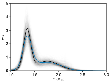
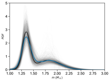
Figure 1: Grey lines represent 1000 posterior samples drawn from the truncated models summarized in Table 2 (left panel) and Table 3 (right panel). The blue curve is the posterior mean distribution and the black line is the maximum posterior distribution.

4.1 Effects on Individual Masses

To investigate the differences between the two models defined above, we analyzed the impact of a uniform distribution for $\cos i$ on the sampling of individual pulsar masses. In the “accuracy-dependent” model, if only $f$ and $m_{t}$ or $q$ are known, the individual masses of pulsars are marginalized from Equations (11) and (12). For the sake of simplicity, we present in the second and third columns of Table 4 the $95\%$ HPDI of masses of four selected systems (namely the pulsars B1957+20, J1311-3430, B1516+02B and J1748-2021B) derived in the “accuracy-dependent” model, using Equations (11) and (12). These systems were known for a long time to be potentially extremely massive ($\geq$2.0 $M_{\odot}$), and are important—although not exclusively—for the inference of $m_{max}$. We now focus our attention on them to illustrate the impact of a flat distribution over $\cos i$ on posterior estimations.

Table 4: Individual pulsar mass of systems listed in this table are sampled from Equations (11) and (12), as functions of the total mass (second column) or mass ratio (third column). They are particularly interesting since their masses derived from observations are $\geq$2.0 $M_{\odot}$ (fourth column).

Pulsar	$m_{mt}~{}[M_{\odot}]$	$m_{q}~{}[M_{\odot}]$	$m_{observations}~{}[M_{\odot}]$
B1957+20	-	1.16–2.14	$2.40\pm 0.12$
J1311-3430	-	1.17–2.14	$2.22\pm 0.10$
B1516+02B	1.26–2.15	-	$2.08\pm 0.19$
J1748-2021B	1.23–2.59	-	$2.74\pm 0.21$

Below, we provide comments on the inferences for each of the four pulsars listed in Table 4. We compare sampled masses with the results obtained from spectrophotometry modeling, summarized in the fourth column. It is worth noting that, for all four pulsars, the masses sampled from the “accuracy-dependent” model are inconsistent with values derived from the original observations (last column).

4.1.1 PSR B1957+20

A black-widow system. Analysis of the light curve of the companion star yields a radial–velocity amplitude of $K_{2}=353\pm 4$ km s^-1. When combined with the pulsar’s mass function, this measurement provides a minimum companion mass of $m_{c,min}=0.022~{}M_{\odot}$. The best-fit values for the mass ratio and inclination angle are $q=69.2\pm 0.8$ and $i=65^{\circ}\pm 2^{\circ}$, respectively. These parameters, when combined, result in a best-fit pulsar mass of $m=2.40\pm 0.12~{}M_{\odot}$ (Van Kerkwijk et al., 2011), and a lower limit on the pulsar mass at $1.66~{}M_{\odot}$. As seen in the third column of Table 4, the “accuracy-dependent” model leads us to a marginalized mass between 1.16–2.14 $M_{\odot}$, inconsistent with spectroscopic determination. As we commented in Section 2.4, the work in Clark et al. (2023) places a constraint of $50^{\circ}<i<85^{\circ}$, resulting in a mean mass at $1.81\pm 0.07~{}M_{\odot}$. Further investigation into the geometry and emissions of spider systems is necessary to pinpoint the correct mass value.

4.1.2 PSR J1311-3430

Until recently, the mass of this black-widow system was determined using a light-curve analysis, resulting in a mass of $m=2.63^{+0.3}_{-0.2}~{}M_{\odot}$ Romani et al. (2012). However, constraints on the inclination angle $i$ were poor. More recently, Kandel and Romani (2022) conducted an analysis of heating models for the light curve, leading to improved determinations of the NS masses. In their preferred model, the inclination angle is estimated to be $i=68.7^{\circ}\pm 2.1^{\circ}$. With a radial velocity amplitude of $K_{2}=641.2\pm 3.6$ and a companion mass of $m_{c}=0.012\pm 0.006$, the pulsar’s mass is inferred to be $m=2.22\pm 0.10~{}M_{\odot}$, above the $95\%HPDI$ derived in the “accuracy-dependent” model.

4.1.3 PSR B1516+02B

This pulsar is located in the globular cluster NGC 5904 and is part of a binary system with a companion that is either a WD or a low-mass main sequence (MS) star. The binary system has a total mass of $2.29\pm 0.17~{}M_{\odot}$, leading to a best-fit pulsar mass estimate of $m=2.08\pm 0.19~{}M_{\odot}$ (Freire et al., 2008). There is a $90\%$ probability that the pulsar’s mass is greater than $1.82~{}M_{\odot}$, and a $0.77\%$ probability that the inclination angle is low enough for the pulsar’s mass to fall within the range of 1.20–1.44 $M_{\odot}$.

4.1.4 PSR J1748-2021B

This pulsar is part of a massive binary system with a total mass of $2.92\pm 0.20~{}M_{\odot}$, which was obtained from precise measurements of $\dot{\omega}$ under the assumption of a fully relativistic system (Freire et al., 2008). The probability that the pulsar’s mass falls within the range of 1.20–1.44 $M_{\odot}$ is only $0.10\%$, requiring an extremely low orbital inclination. The median mass of the companion star is estimated to be 0.142 with lower and upper 1$\sigma$ limits at 0.124 and 0.228 $M_{\odot}$, respectively. This range of companion masses suggests that the companion star could be a WD or a non-evolved MS star, which implies a pulsar mass of $2.74~{}M_{\odot}$.

4.2 Effects on the Maximum Mass

We now proceed to investigate the impact of a uniform distribution for $\cos i$ on the posterior distribution of $m_{max}$. Following the approach of Alsing et al. (2018) and Shao et al. (2020), we obtained the marginalized posterior distribution shown by the solid line in the left panel of Figure 2, with a maximum of $\sim$2.2 $M_{\odot}$. On the other hand, the marginalized posterior distribution for the model where all pulsars are assumed to be normally distributed (“accuracy-independent” model) is shown by the solid line in the right panel of Figure 2, with a maximum of around $2.6~{}M_{\odot}$. In addition to the maximum values that differ considerably between the two treatments, the shape of the $m_{max}$ distribution changes significantly too, as we can see in Figure 2.

For both models, we verified the impact of changing the masses of PSR B1957+20, PSR J1048+2339, PSR J1555-2908, and PSR J2129-0429 by the values derived from $\gamma$-ray observations, listed in Table 1. Since in the analysis of Clark et al. (2023) the only value that changed considerably compared to previous estimates was that of PSR B1957+20, we did not expect a significant change in the overall results, as confirmed by the dashed line in both panels of Figure 2. Only the amplitude is mildly affected, but the point estimates for the distributions remain the same.

In the subsequent analysis, we examined the impact of changing the treatment of individual pulsar masses in the “accuracy-dependent” model for the four systems mentioned in the previous section (PSR B1957+20, PSR J1311-3430, PSR B1516+02B, PSR J1748-2021B). In order to do that, we kept the treatment described in Section 3.1 for all systems, with the exception of those mentioned above, which are now also assumed to follow a normal distribution. The result is shown by the dot-dashed line in the left panel of Figure 2. By changing the likelihood treatment for only these particular systems, the marginalized distribution of $m_{max}$ shifts to the right, and the probability of higher $m_{max}$ values is increased. The dot-dashed line in the left panel tends to the solid line in the right panel as we assume more systems to be modeled with Gaussians, and equalizes when all systems are treated as Gaussian. As we can note, the lower individual mass estimates obtained when a flat distribution over $i$ is invoked (and discussed in Section 4.1) are reflected, consequently, in a lower estimation of $m_{max}$.

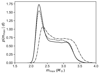
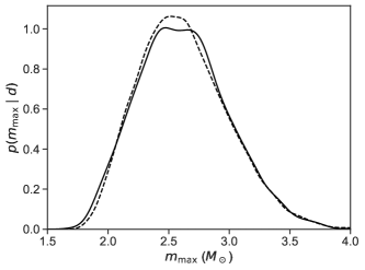
Figure 2: Marginal posterior distribution of $m_{max}$ sampled from the “accuracy-dependent” model (left panel) and the “accuracy-independent” model (right panel). The solid line represents the analysis assuming the individual pulsars to be sampled from 3 types of likelihoods (left panel), and to be sampled from normal distributions only (right panel). In the dashed curve, we analyze the effect of assuming the masses found from $\gamma$-ray observations, listed in Table 1.

As demonstrated, the prior assumption regarding the orbital inclination angle significantly influences the determination of the mass limits, emphasizing the importance of a cautious approach. The high amplitude of values close to $2~{}M_{\odot}$ in the left panel of Figure 2 is a consequence of lower estimates of individual masses found in this particular approach, leading to a density accumulation around $2~{}M_{\odot}$ and a significant decrease in the probability for values $\geq 2.4~{}M_{\odot}$.

In this scenario, the “accuracy-independent” model is preferred, since the individual sampled masses are consistent with values derived from observations. The ideal scenario, however, would involve the adoption of the “accuracy-dependent” model, with consideration of observational constraints on the inclination angle ($i$) for each binary system. This meticulous treatment remains a subject for a future work.

4.3 Posterior Predictive Check

In Bayesian analysis, a crucial step to validate a model is to assess whether predictive simulated data resemble the observed data. In essence, we aim to understand whether new observations drawn from the posterior distribution would be consistent with the existing observed sample. Any significant disparity might indicate a misfit. This analytical process is known as a posterior predictive check (PPC). One approach to conducting a PPC is to visually compare summaries of real data with those of simulated data. In addition, it can be valuable to quantitatively assess the level of discrepancy. This can be achieved by defining a “test quantity” ($T$), often chosen as the mean, and calculating a Bayesian p-value. This p-value indicates the probability that the test quantity of simulated data ($T^{sim}$) exceeds the observed test quantity ($T$):

$$p=P(T(m^{sim})>T(m)|m).$$ (13)

Following the detection of GW170817, several studies Ai et al. (2020); Rezzola et al. (2018); Margalit and Metzger (2017); Ruiz et al. (2018); Shibata et al. (2019) derived mass limits for NSs based on observational constraints set by the GW event. All these analyses resulted in maximum masses that are significantly lower than the $m_{max}$ we found for the “accuracy-independent” model.

Our goal is to investigate the maximum value of the distribution and, faced with the substantial differences we have identified for this quantity between the two models we treated here and with the values derived from GW data, we sought further investigation to determine which value of $m_{max}$ complies with the available sample of NS masses. Consider that we are analyzing a distribution without specifying that it has to be truncated, the question we want to address is: what would be the value consistent with an upper threshold for this distribution?

For this purpose, we conducted a new MCMC sampling from a non-truncated Gaussian mixture, with a normal likelihood for all pulsars. The only difference to the previous model is the absence of the denominator in Equation (10). In Table 5, we summarize the mean and standard deviation of each model parameter.

Table 5: Summary of marginal posterior distribution of each parameter in the non-truncated bimodal model. These results were used to generate 10,000 synthetic bimodal Gaussian distributions.

$r_{1}$	$r_{2}$	$\mu_{1}$	$\mu_{2}$	$\sigma_{1}$	$\sigma_{2}$
$0.527\pm 0.090$	$0.473\pm 0.090$	$1.354\pm 0.026$	$1.801\pm 0.070$	$0.095\pm 0.023$	$0.301\pm 0.037$

Using the mean values reported in Table 5, we then generated 10,000 posterior predictive distributions using the software MATHEMATICA Wolfram Research Inc. . Subsequently, we defined the test quantity, $T$, as the number of elements in the observed sample with masses exceeding a specific value, referred to as “$m_{max}$”. This approach enables us to examine the upper limit for the distribution. The p-value is derived from the number of times $T^{sim}>T$. To illustrate, the top left panel in Figure 3 offers insight into the probability of detecting new objects with $m>2.09~{}M_{\odot}$ in future observations, which is $47.8\%$, a high value. A p-value close to zero is consistent with a mass limit, i.e., a low p-value implies a reduced probability of detecting new objects with masses exceeding the associated value. Through this alternative analysis, we confirm that the distribution of galactic NSs supports high $m_{max}$ values, such as the $2.6~{}M_{\odot}$ we found from the “accuracy-independent” model.

It is important to note that in this analysis all masses were modeled with Gaussians. An inconsistency between results found through the PPC and through the “accuracy-independent” model would also reveal a flaw in the “accuracy-independent” model, which is not the case. This analysis is not intended to be conclusive, but rather complementary.

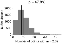
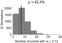
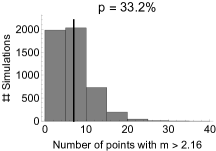
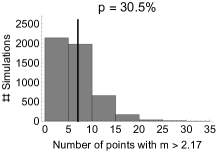
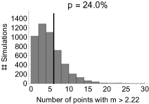
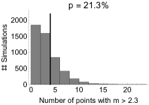
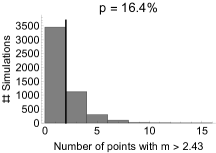
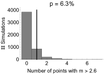
Figure 3: Posterior predictive check on the two-Gaussian model without truncation. The purpose is to investigate the tail of distributions. High p-values indicate that values higher than the one specified in the label are very common, thus they cannot be pointed to as valid thresholds. The adopted $m_{max}$ from NS–NS mergers are, from left to right and top to bottom, Ai et al. (2020) with $2.09^{+0.11}_{-0.09}~{}M_{\odot}$; Shao et al. (2020) with $2.13^{+0.08}_{-0.07}~{}M_{\odot}$; Rezzola et al. (2018) with $2.16^{+0.17}_{-0.15}~{}M_{\odot}$; Margalit and Metzger (2017) with $2.17~{}M_{\odot}$; Ruiz et al. (2018) with 2.16–2.28 $M_{\odot}$; Shibata et al. (2019) with $2.3~{}M_{\odot}$; Ai et al. (2020) with $2.43^{+0.10}_{-0.08}~{}M_{\odot}$. The last panel represents our result for the “accuracy-independent” model. We used the mean value of each referenced work, since they cover the whole range of high masses reasonably well.

5 Discussions and Conclusions

The old idea of a unique formation channel for NSs and the existence of a canonical mass have long been invalidated, possibly pointing towards a variety of formation mechanisms, including electron capture supernova and accretion-induced collapses. The current debate revolves around whether the mass limit supported by NSs is above or below the range of 2.2–2.3 $M_{\odot}$.

Recent analyses of the galactic sample of NSs have found evidence for a sharp cut-off at $m_{max}<2.3~{}M_{\odot}$ Alsing et al. (2018); Shao et al. (2020), even though the number of high-mass estimates in observed NSs continues to grow. The most recent addition to this sample is PSR J0952-0607, with a reported mass of $2.35\pm 0.17~{}M_{\odot}$ Romani et al. (2022). On the other hand, observations from the gravitational wave event, GW170817, have also played a crucial role in constraining the mass limit, with results falling in the interval between 2.1 and $2.3~{}M_{\odot}$ Ai et al. (2020); Shao et al. (2020); Rezzola et al. (2018); Margalit and Metzger (2017); Ruiz et al. (2018); Shibata et al. (2019), in line with previous galactic analyses. However, the detection of the GW190814 signal, originating from the merger of a $23~{}M_{\odot}$ BH with an unidentified $m=2.59_{-0.09}^{+0.08}~{}M_{\odot}$ companion, raised a new tension. An analysis of the BBH merging population, performed by the LV team Abbott et al. (2021), found the GW190814 to be an outlier, i.e., it is potentially associated with an NS–BH merger. In addition, a maximum mass constraint for non-spinning NSs was also derived from the available LV sample of NS–BH events, with a result of $2.7^{+0.5}_{-0.4}~{}M_{\odot}$ (Ye and Fishbach, 2022). More recently, an analysis combining as many astronomical observations as possible led to a preferred threshold value of 2.49–2.52 $M_{\odot}$ Ai et al. (2023), while Fan et al. (2023) placed a minimum of $2.25^{+0.08}_{-0.07}~{}M_{\odot}$ to $M_{TOV}$, two completely independent pieces of evidence, to solve the puzzle of the maximum mass value.

To address this ongoing tension, we performed in this work an analysis of the mass distribution of galactic NSs to investigate the impact of the assumption of a uniform distribution between 0 and 1, associated with the orbital inclination angle $i$. As previously mentioned, this parameter is responsible for the largest uncertainties in mass measurements and requires careful consideration. Our findings reveal that this uniform assumption results in individual sampled masses that fall below the constraints set from observational modeling (see Section 4.1). As a consequence, the distribution threshold $m_{max}$ also shows a preference for lower values, at $\sim$2.2 $M_{\odot}$.

In the “accuracy-independent” model, all pulsars are modeled as normal distributions. The mass values reported in Table 7 were derived while taking into account observational constraints at $i$, which in turn can be model-dependent. This approach is consistent with a scenario favoring the existence of extremely massive NSs ($\sim$2.6 $M_{\odot}$). A complementary analysis (PPC in Section 3) strengthens the possibility of a high $m_{max}$ for the galactic population, in line with a few conclusions derived from GW analyses, mentioned throughout this work. The discrepancy between the two approaches we treat in this work revealed that it is necessary to be careful when making assumptions over $i$, since different hypotheses over this quantity can lead to drastically different pulsar masses, consequently influencing the $m_{max}$ determination. An ideal approach would involve implementing the “accuracy-dependent” model while accounting for the distribution of $i$ for each particular system, constrained from observational data, as performed for the case of black hole masses in de Sá et al. (2023), where each object was analyzed individually and it was checked that the different Keplerian parameter values employed in each mass estimate did not rely on inconsistent assumptions. A similar treatment for NS masses remains a subject for future work.

Although determining the orbital inclination of a pulsar binary is a challenging task, we showed in this work that the constraints obtained from observations are crucial information about the system and must be treated accordingly. Whether the adopted spectrophotometric model adopted to set these constraints is the ideal or not is another question and needs to be investigated further. The work of Clark et al. (2023), if confirmed by future research, can help solve the problem of NS mass accuracy, providing a solution to the NS maximum mass puzzle, which in turn has strong consequences for the supranuclear equation of state. But for now, based on the galactic sample, we cannot rule out the possibility that extremely massive NSs ($m>2.3~{}M_{\odot}$) exists in nature.

Conceptualization, L.S.R. and J.E.H.; methodology, L.S.R.; software, L.S.R.; validation, L.S.R. and L.M.d.S.; formal analysis, L.S.R. and L.M.d.S.; data curation, L.S.R.; writing—original draft preparation, L.S.R. and J.E.H.; writing—review and editing, L.G.B., G.Y.C., and M.G.B.d.A. All authors have read and agreed to the published version of the manuscript.

This research was funded by FAPESP Agency (São Paulo State) grant number 2020/08518-2. L.S.R was funded by Capes Agency (Brazil). L.M.S. received funding from the CNPq (Brazil), grant number 140794/2021-2.

Not applicable.

Not applicable.

Data are contained within the > article.

The authors declare no conflicts of interest. The funding agencies had no role in the design of the study; in the collection, analyses, or interpretation of data; in the writing of the manuscript; or in the decision to publish the results.

Abbreviations The following abbreviations are used in this manuscript:

NS	Neutron Star
GR	General Relativity
Fe	Iron
TOV	Tolman-Oppenheimer-Volkoff
EoS	Equation of state
BH	Black Hole
O-Ne-Mg	Oxygen-Neon-Magnesium
AIC	Accretion-Induced-Collapse
WD	White-Dwarf
GW	Gravitational Wave
LV	LIGO-Virgo
BBH	Binary Black Hole
ToA	Time of arrival
NICER	Neutron star Interior Composition ExploreR
pK	post-Keplerian
DNS	Double Neutron Star
MCMC	Markov Chain Monte Carlo
HPDI	Highest posterior density interval
MS	Main sequence
PPC	Posterior predictive check

yes

Appendix A Sample of Neutron Stars

The complete sample of NSs with mass constraints is displayed in the Table below.

In the “accuracy-dependent” model, for systems where $f$ and $m_{t}$ of $q$ values are reported, we have used them to marginalize individual pulsar masses through Equations (11) and (12). For the “accuracy-independent” model we sampled pulsar’s mass with values provided in the 6th column of Table 7. The three systems without individual mass constraints were left out from the second analysis. Since they are DNS systems, recognized to have a distribution way below $2~{}M_{\odot}$, they do not contribute significantly for the $m_{max}$ inference. Furthermore, for DNS systems without precise constraints on individual masses (from J1018-1523 to J2140-2311B), we considered only the mass of the pulsar component.

Table 6: Neutron star measurements for 125 binary systems, with $1\sigma$ uncertainties.

Pulsar	Type	$f$ [$M_{\odot}$]	$m_{t}$ [$M_{\odot}$]	$q$	$m_{p}$ [$M_{\odot}$]	Reference
2S 0921-630	x-ray/optical				1.44 $\pm$ 0.1	Steeghs and Jonker (2007)
4U 1538-522	x-ray/optical				1.02 $\pm$ 0.17	Falanga et al. (2015)
4U 1608-52	x-ray/optical				1.57 $\pm$ 0.29	Ozel et al. (2016)
4U 1700-377	x-ray/optical				1.96 $\pm$ 0.19	Falanga et al. (2015)
4U 1702-429	x-ray/optical				1.9 $\pm$ 0.3	Nattila et al. (2017)
4U 1724-207	x-ray/optical				1.81 $\pm$ 0.31	Ozel et al. (2016)
4U 1820-30	x-ray/optical				1.77 $\pm$ 0.27	Ozel et al. (2016)
4U 1822-371	x-ray/optical				1.96 $\pm$ 0.36	Munoz-Darias et al. (2005)
Cen X-3	x-ray/optical				1.57 $\pm$ 0.16	Falanga et al. (2015)
Cyg X-2	x-ray/optical				1.71 $\pm$ 0.21	Casares et al. (2010)
EXO 0748-676	x-ray/optical				2.01 $\pm$ 0.21	Knight et al. (2022)
EXO 1722-363	x-ray/optical				1.91 $\pm$ 0.45	Falanga et al. (2015)
EXO 1745-248	x-ray/optical				1.65 $\pm$ 0.26	Ozel et al. (2016)
Her X-1	x-ray/optical				1.073 $\pm$ 0.358	Rawls et al. (2011)
J013236.7+303228	x-ray/optical				2.0 $\pm$ 0.4	Bhalerao et al. (2012)
J0212.1+5320	x-ray/optical				1.85 $\pm$ 0.29	Shahbaz et al. (2017)
J0427.9-6704	x-ray/optical				1.86 $\pm$ 0.11	Strader et al. (2019)
J0846.0+2820	x-ray/optical				1.96 $\pm$ 0.41	Strader et al. (2019)
J0952-0607	x-ray/optical				2.35 $\pm$ 0.17	Romani et al. (2022)
J1023+0038	x-ray/optical				1.65 $\pm$ 0.16	Strader et al. (2019)
J1048+2339	x-ray/optical				1.96 $\pm$ 0.22	Strader et al. (2019)
J1301+0833	x-ray/optical				1.60 $\pm$ 0.23	Kandel and Romani (2022)
J1311-3430	x-ray/optical				$2.22\pm 0.10$	Kandel and Romani (2022)
J1417.7-4407	x-ray/optical				1.62 $\pm$ 0.3	Strader et al. (2019)
J1555-2908	x-ray/optical				1.67 $\pm$ 0.06	Kennedy et al. (2022)
J1653-0158	x-ray/Optical				2.15 $\pm$ 0.16	Kandel and Romani (2022)
J1723-2837	x-ray/optical				$1.22\pm 0.23$	Strader et al. (2019)
J1810+1744	x-ray/Optical				2.13 $\pm$ 0.04	Kandel and Romani (2022)
J2039.6-5618	x-ray/optical				2.04 $\pm$ 0.31	Strader et al. (2019)
J2129-0429	x-ray/optical				1.74 $\pm$ 0.18	Strader et al. (2019)
J2215+5135	x-ray/optical				2.28 $\pm$ 0.10	Kandel and Romani (2020)
J2339-0533	x-ray/optical				1.47 $\pm$ 0.09	Kandel et al. (2020)
KS 1731-260	x-ray/optical				1.61 $\pm$ 0.37	Ozel et al. (2016)
LMC X-4	x-ray/optical				1.57 $\pm$ 0.11	Falanga et al. (2015)
OAO 1657-415	x-ray/optical				1.74 $\pm$ 0.3	Falanga et al. (2015)
SAX 1748.9-2021	x-ray/optical				1.81 $\pm$ 0.31	Ozel et al. (2016)
SAX J1802.7-2017	x-ray/optical				1.57 $\pm$ 0.25	Falanga et al. (2015)
SMC X-1	x-ray/optical				1.21 $\pm$ 0.12	Falanga et al. (2015)
Vela X-1	x-ray/optical				2.12 $\pm$ 0.16	Falanga et al. (2015)
XTE J1855-026	x-ray/optical				1.41 $\pm$ 0.24	Falanga et al. (2015)
XTE J2123-058	x-ray/optical				1.53 $\pm$ 0.36	Casares et al. (2002)
B1957+20	x-ray/optical	0.005		69.2 $\pm$ 0.8	$2.4\pm 0.12$	Van Kerkwijk et al. (2011)
J1740-5350	x-ray/optical	0.002644		5.85 $\pm$ 0.13	1.6$\pm$0.3	Ferraro et al. (2003)
J1816+4510	x-ray/optical	0.0017607		9.54 $\pm$ 0.21	1.45 $\pm$ 0.38	Kaplan et al. (2013)
B1534+12	NS-NS				1.3332 $\pm$ 0.0010	Fonseca et al. (2014)
B1534+12 Cp	NS-NS				1.3452 $\pm$ 0.0010	Fonseca et al. (2014)
B1913+16	NS-NS				1.438 $\pm$ 0.001	Weisberg and Huang. (2016)
B1913+16 Cp	NS-NS				1.390 $\pm$ 0.001	Weisberg and Huang. (2016)
B2127+11C	NS-NS				1.358 $\pm$ 0.010	Jacoby et al. (2006)
B2127+11C Cp	NS-NS				1.354 $\pm$ 0.010	Jacoby et al. (2006)
J0453+1559	NS-NS				1.559 $\pm$ 0.004	Martinez et al.; (2015)
J0453+1559 Cp	NS-NS				1.174 $\pm$ 0.004	Martinez et al.; (2015)
J0509+3801	NS-NS				1.34 $\pm$ 0.08	Lynch et al. (2012)
J0509+3801 Cp	NS-NS				1.46 $\pm$ 0.08	Lynch et al. (2012)
J0514-4002A	NS-NS				1.25 $\pm$ 0.05	Ridolfi et al. (2019)
J0514-4002A Cp	NS-NS				1.22 $\pm$ 0.05	Ridolfi et al. (2019)
J0737-3039A	NS-NS				1.338185 $\pm$ 0.000013	Kramet et al. (2021)
J0737-3039B	NS-NS				1.248868 $\pm$ 0.000012	Kramet et al. (2021)
J1756-2251	NS-NS				1.341 $\pm$ 0.007	Ferdman et al. (2014)
J1756-2251 Cp	NS-NS				1.230 $\pm$ 0.007	Ferdman et al. (2014)
J1757-1854	NS-NS				1.3406 $\pm$ 0.0005	Cameron et al. (2023)
J1757-1854 Cp	NS-NS				1.3922 $\pm$ 0.0005	Cameron et al. (2023)
J1807-2500B	NS-NS				1.3655 $\pm$ 0.0021	Lynch et al. (2012)
J1807-2500B Cp	NS-NS				1.2064 $\pm$ 0.0020	Lynch et al. (2012)
J1829+2456	NS-NS				1.306 $\pm$ 0.007	Haniewicz et al. (2021)
J1829+2456 Cp	NS-NS				1.299 $\pm$ 0.007	Haniewicz et al. (2021)

Table 7: Cont.

Pulsar	Type	$f$ [$M_{\odot}$]	$m_{t}$ [$M_{\odot}$]	$q$	$m_{p}$ [$M_{\odot}$]	Reference
J1906+0746	NS-NS				1.291 $\pm$ 0.011	Van Leeuwen et al. (2015)
J1906+0746 Cp	NS-NS				1.322 $\pm$ 0.011	Van Leeuwen et al. (2015)
J1913+1102	NS-NS				1.62 $\pm$ 0.03	Ferdman et al. (2020)
J1913+1102 Cp	NS-NS				1.27 $\pm$ 0.03	Ferdman et al. (2020)
J1018-1523	NS-NS	0.238062	2.3 $\pm$ 0.3			Swiggum et al. (2023)
J1325-6253	NS-NS	0.1415168	2.57 $\pm$ 0.06		1.37 $\pm$ 0.27	Sengar et al. (2022)
J1411+2551	NS-NS	0.1223898	2.538 $\pm$ 0.022			Martinez et al. (2017)
J1759+5036	NS-NS	0.081768	2.62 $\pm$ 0.03		1.52 $\pm$ 0.26	Agazie et al. (2021)
J1811-1736	NS-NS	0.128121	2.57 $\pm$ 0.10		1.34 $\pm$ 0.16	Corongiu et al. (2007)
J1930-1852	NS-NS	0.34690765	2.54 $\pm$ 0.03			Swiggum et al. (2015)
J1946+2052	NS-NS	0.268184	2.50 $\pm$ 0.04		1.25 $\pm$ 0.15	Stovall et al. (2018)
J2140-2311B	NS-NS	0.2067	2.53 $\pm$ 0.08		1.3 $\pm$ 0.2	Balakrishinan et al. (2023)
B1855+09	NS-WD				1.54 $\pm$ 0.13	Reardon et al. (2021)
J0337+1715	NS-WD				1.4401 $\pm$ 0.0015	Voisin et al. (2020)
J0348+0432	NS-WD				2.01 $\pm$ 0.04	Antoniadis et al. (2016)
J0437-4715	NS-WD				1.44 $\pm$ 0.07	Reardon et al. (2016)
J0621+1002	NS-WD				1.53 $\pm$ 0.15	Kasian (2012)
J0740+6620	NS-WD				2.08 $\pm$ 0.07	Fonseca et al. (2021)
J0751+1807	NS-WD				1.64 $\pm$ 0.15	Desvignes et al. (2016)
J0955-6150	NS-WD				1.71 $\pm$ 0.03	Serylak et al. (2022)
J1012+5307	NS-WD				1.72 $\pm$ 0.16	Mata-Sánchez et al. (2020)
J1017-7156	NS-WD				$2.0\pm 0.8$	Reardon et al. (2021)
J1022-1001	NS-WD				$1.44\pm 0.44$	Reardon et al. (2021)
J1125-6014	NS-WD				1.68 $\pm$ 0.16	Shamohammadi et al. (2022)
J1141-6545	NS-WD				1.27 $\pm$ 0.01	Bhat et al. (2008)
J1528-3146	NS-WD				1.61 $\pm$ 0.14	Berthereau et al. (2023)
J1600-3053	NS-WD				2.06 $\pm$ 0.42	Reardon et al. (2021)
J1614-2230	NS-WD				1.94 $\pm$ 0.03	Shamohammadi et al. (2022)
J1713+0747	NS-WD				1.28 $\pm$ 0.08	Reardon et al. (2021)
J1738+0333	NS-WD				1.47 $\pm$ 0.07	Antoniadis et al. (2012)
J1741+1351	NS-WD				1.14 $\pm$ 0.34	Kirichenko et al. (2020)
J1748-2446am	NS-WD				1.649 $\pm$ 0.074	Andersen and Ransom et al. (2018)
J1802-2124	NS-WD				1.24 $\pm$ 0.11	Ferdman et al. (2010)
J1811-2405	NS-WD				2.0 $\pm$ 0.65	Ng et al. (2020)
J1909-3744	NS-WD				1.45 $\pm$ 0.03	Shamohammadi et al. (2022)
J1910-5958A	NS-WD				1.55 $\pm$ 0.07	Corongiu et al. (2023)
J1918-0642	NS-WD				1.29 $\pm$ 0.10	Arzoumanian et al. (2018)
J1933-6211	NS-WD				1.40 $\pm$ 0.25	Geyer et al. (2023)
J1946+3417	NS-WD				1.828 $\pm$ 0.022	Barr et al. (2017)
J1949+3106	NS-WD				1.34 $\pm$ 0.16	Zhu et al. (2019)
J1950+2414	NS-WD				1.496 $\pm$ 0.023	Zhu et al. (2019)
J1959+2048	NS-WD				2.18 $\pm$ 0.09	Kandel and Romani (2020)
J2043+1711	NS-WD				1.38 $\pm$ 0.13	Arzoumanian et al. (2018)
J2045+3633	NS-WD				1.251 $\pm$ 0.021	McKee et al. (2020)
J2053+4650	NS-WD				1.40 $\pm$ 0.21	Berezina et al. (2017)
J2222-0137	NS-WD				1.831 $\pm$ 0.010	Guo et al. (2021)
J2234+0611	NS-WD				1.353 $\pm$ 0.016	Stovall et al. (2019)
B1516+02B	NS-WD	0.000646723	2.29 $\pm$ 0.17		$2.08\pm 0.19$	Freire et al. (2008)
B1802-07	NS-WD	0.00945034	1.62 $\pm$ 0.07		$1.26\pm 0.13$	Thorsett and Chakrabarty (1999)
B2303+46	NS-WD	0.246261924525	2.64 $\pm$ 0.05		$1.38\pm 0.08$	Thorsett and Chakrabarty (1999)
J0024-7204H	NS-WD	0.001927	1.665 $\pm$ 0.007		1.41 $\pm$ 0.08	Freire et al. (2017, 2003)
J1748-2021B	NS-WD	0.0002266235	2.69 $\pm$ 0.071		$2.74\pm 0.21$	Freire et al. (2008)
J1748-2446I	NS-WD	0.003658	2.17 $\pm$ 0.02		$1.91\pm 0.06$	Kiziltan et al. (2013)
J1748-2446J	NS-WD	0.013066	2.20 $\pm$ 0.04		$1.79\pm 0.06$	Kiziltan et al. (2013)
J1750-37A	NS-WD	0.0518649	1.97 $\pm$ 0.15		$1.26\pm 0.37$	Freire et al. (2008)
J1823-3021G	NS-WD	0.0123	2.65 $\pm$ 0.07		2.1 $\pm$ 0.2	Ridolfi et al. (2021)
J1824-2452C	NS-WD	0.006553	1.616 $\pm$ 0.007		$1.31\pm 0.25$	Bégin (2006)
J0045-7319	NS-MS				1.58 $\pm$ 0.34	Thorsett and Chakrabarty (1999)
J1903+0327	NS-MS				1.667 $\pm$ 0.016	Arzoumanian et al. (2018)

[custom]

References

References

- Hewish (1968) Hewish, A. Pulsars. Sci. Am. 1968, 219, 25–35.
- Kramet et al. (2021) Kramer, M.; Stairs, I.H.; Manchester, R.N.; Wex, N.; Deller, A.T.; Coles, W.A.; Ali, M.; Burgay, M.; Camilo, F.; Cognard, I.; et al. Strong-field gravity tests with the double pulsar. Phys. Rev. X 2021 11, 041050.
- Baade & Zwicky (1934) Baade, W.; Zwicky, F. On super-novae. Proc. Natl. Acad. Sci. USA 1934, 20, 254–259.
- Cameron (1959) Cameron, A.G. Neutron Star Models. Astrophys. J. 1959, 130, 884.
- Nomoto (1984) Nomoto, K. Evolution of 8–10 solar mass stars toward electron capture supernovae. I-Formation of electron-degenerate O+ NE+ MG cores. Astrophys. J. 1984, 277, 791–805.
- Finn (1994) Finn, L.S. Observational constraints on the neutron star mass distribution. Phys. Rev. Lett. 1994, 73, 1878.
- Rhoades and Ruffini (1974) Rhoades, C.E., Jr.; Ruffini, R. Maximum mass of a neutron star. Phys. Rev. Lett. 1974, 32, 324.
- Thorsett and Chakrabarty (1999) Thorsett, S.E.; Chakrabarty, D. Neutron star mass measurements. i. radio pulsars. Astrophys. J. 1999, 512, 288.
- Barziv et al. (2001) Barziv, O.; Kaper, L.; Van Kerkwijk, M.H.; Telting, J.H.; Van Paradijs, J. The mass of the neutron star in Vela X-1. Astron. Astrophys. 2001, 377, 925–944.
- Nice et al. (2005) Nice, D.J.; Splaver, E.M.; Stairs, I.H.; Löhmer, O.; Jessner, A.; Kramer, M.; Cordes, J.M. A 2.1 Pulsar Measured by Relativistic Orbital Decay. Astrophys. J. 2005, 634, 1242.
- Freire et al. (2008) Freire, P.C.C.; Wolszczan, A.; van den Berg, M.; Hessels, J.W.T. A massive neutron star in the globular cluster M5. Astrophys. J. 2008, 679, 1433.
- Freire et al. (2008) Freire, P.C.C.; Ransom, S.M.; Bégin, S.; Stairs, I.H.; Hessels, J.W.T.; Frey, L.H.; Camilo, F. Eight new millisecond pulsars in NGC 6440 and NGC 6441. Astrophys. J. 2008, 675, 670.
- Demorest et al. (2010) Demorest, P.B.; Pennucci, T.; Ransom, S.M.; Roberts, M.S.E.; Hessels, J.W.T. A two-solar-mass neutron star measured using Shapiro delay. Nature 2010, 467, 1081–1083.
- Cromartie et al. (2020) Cromartie, H.T.; Fonseca, E.; Ransom, S.M.; Demorest, P.B.; Arzoumanian, Z.; Blumer, H.; Brook, P.R.; DeCesar, M.E.; Dolch, T.; Ellis, J.A.; et al. Relativistic Shapiro delay measurements of an extremely massive millisecond pulsar. Nat. Astron. 2020, 4, 72–76.
- Schwab et al. (2010) Schwab, J.; Podsiadlowski, P.; Rappaport, S. Further evidence for the bimodal distribution of neutron-star masses. Astrophys. J. 2010, 719, 722.
- Podsiadlowski et al. (2004) Podsiadlowski, P.; Langer, N.; Poelarends, A.J.T.; Rappaport, S.; Heger, A.; Pfahl, E. The effects of binary evolution on the dynamics of core collapse and neutron star kicks. Astrophys. J. 2004, 612, 1044.
- Hiramatsu et al. (2021) Hiramatsu, D.; Howell, D.A.; Van Dyk, S.D.; Goldberg, J.A.; Maeda, K.; Moriya, T.J.; Tominaga, N.; Nomoto, K.; Hosseinzadeh, G.; Arcavi, I.; et al. The electron-capture origin of supernova 2018zd. Nat. Astron. 2021, 5, 903–910.
- Zhang et al. (2011) Zhang, C.M.; Wang, J.; Zhao, Y.H.; Yin, H.X.; Song, L.M.; Menezes, D.P.; Wickramasinghe, D.T.; Ferrario, L.; Chardonnet, P. Study of measured pulsar masses and their possible conclusions. Astron. Astrophys. 2011, 527, A83.
- Valentim et al. (2011) Valentim, R.; Rangel, E.; Horvath, J.E. On the mass distribution of neutron stars. Mon. Not. R. Astron. Soc. 2011, 414, 1427–1431.
- Kiziltan et al. (2013) Kiziltan, B.; Kottas, A.; De Yoreo, M.; Thorsett, S.E. The neutron star mass distribution. Astrophys. J. 2013, 778, 66.
- Ozel & Freire (2016) Özel, F.; Freire, P. Masses, radii, and the equation of state of neutron stars. Annu. Rev. Astron. Astrophys. 2016, 54, 401–440.
- Burrows & Varanyan (2021) Burrows, A.; Vartanyan, D. Core-collapse supernova explosion theory. Nature 2021, 589, 29–39.
- Suwa et al. (2018) Suwa, Y.; Yoshida, T.; Shibata, M.; Umeda, H.; Takahashi, K. On the minimum mass of neutron stars. Mon. Not. R. Astron. Soc. 2018, 481, 3305–3312.
- Kandel and Romani (2022) Kandel, D.; Romani, R.W. An Optical Study of the Black Widow Population. Astrophys. J. 2022, 942, 6.
- Linares (2019) Linares, M. Super-Massive Neutron Stars and Compact Binary Millisecond Pulsars. In Proceedings of the XIII Multifrequency Behaviour of High Energy Cosmic Sources Workshop, Palermo, Italy, 3 June 2019.
- Horvath et al. (2020) Horvath, J.E.; Bernardo, A.; Rocha, L.S.; Valentim, R.; Moraes, P.H.R.S.; de Avellar, M.G.B. Redback/Black Widow Systems as progenitors of the highest neutron star masses and low-mass Black Holes. Sci. China Phys. Mech. Astron. 2020, 63, 129531.
- Romani et al. (2022) Romani, R.W.; Kandel, D.; Filippenko, A.V.; Brink, T.G.; Zheng, W. PSR J0952-0607: The Fastest and Heaviest Known Galactic Neutron Star. Astrophys. J. Lett. 2022, 934, L18.
- Wang and Liu (2020) Wang, B.; Liu, D. The formation of neutron star systems through accretion-induced collapse in white-dwarf binaries. Res. Astron. Astrophys. 2020, 20, 135.
- Zhong et al. (2023) Zhong, S.Q.; Li, L.; Dai, Z.G. GRB 211211A: A Neutron Star–White Dwarf Merger? Astrophys. J. Lett. 2023, 947, L21.
- Abbott et al. (2017) Abbott, B.P.; Abbott, R.; Abbott, T.D.; Acernese, F.; Ackley, K.; Adams, C.; Adams, T.; Addesso, P.; Adhikari, R.X.; Adya, V.B.; et al. GW170817: Observation of gravitational waves from a binary neutron star inspiral. Phys. Rev. Lett. 2017, 119, 161101.
- Margalit and Metzger (2017) Margalit, B.; Metzger, B.D. Constraining the maximum mass of neutron stars from multi-messenger observations of GW170817. Astrophys. J. Lett. 2017, 850, L19.
- Alsing et al. (2018) Alsing, J.; Silva, H.O.; Berti, E. Evidence for a maximum mass cut-off in the neutron star mass distribution and constraints on the equation of state. Mon. Not. R. Astron. Soc. 2018, 478, 1377–1391.
- Shibata et al. (2019) Shibata, M.; Zhou, E.; Kiuchi, K.; Fujibayashi, S. Constraint on the maximum mass of neutron stars using GW170817 event. Phys. Rev. D 2019, 100, 023015.
- Shao et al. (2020) Shao, D.-S.; Tang, S.-P.; Jiang, J.-L.; Fan, Y.-Z. Maximum mass cutoff in the neutron star mass distribution and the prospect of forming supramassive objects in the double neutron star mergers. Phys. Rev. D 2020, 102, 063006.
- Shao et al. (2020) Shao, D.-S.; Tang, S.-P.; Sheng, X.; Jiang, J.-L.; Wang, Y.-Z.; Jin, Z.-P.; Fan, Y.-Z.; Wei, D.-M. Estimating the maximum gravitational mass of nonrotating neutron stars from the GW170817/GRB 170817A/AT2017gfo observation. Phys. Rev. D 2020, 101, 063029.
- Abbott et al. (2020) Abbott, R.; Abbott, T.D.; Abraham, S.; Acernese, F.; Ackley, K.; Adams, C.; Adhikari, R.X.; Adya, V.B.; Affeldt, C.; Agathos, M.; et al. GW190814: Gravitational waves from the coalescence of a 23 solar mass black hole with a 2.6 solar mass compact object. Astrophys. J. Lett. 2020, 896, L44.
- Nathanail et al. (2021) Nathanail, A.; Most, E.R.; Rezzolla, L. GW170817 and GW190814: Tension on the Maximum Mass. Astrophys. J. Lett. 2021, 908, L28.
- Abbott et al. (2021) Abbott, R.; Abbott, T.D.; Abraham, S.; Acernese, F.; Ackley, K.; Adams, A.; Adams, C.; Adhikari, R.X.; Adya, V.B.; Affeldt, C. Population properties of compact objects from the second LIGO–Virgo gravitational-wave transient catalog. Astrophys. J. Lett. 2021, 913, L7.
- Ye and Fishbach (2022) Ye, C.; Fishbach, M. Inferring the Neutron Star Maximum Mass and Lower Mass Gap in Neutron Star–Black Hole Systems with Spin. Astrophys. J. 2022, 937, 73.
- Ai et al. (2023) Ai, S.; Gao, H.; Yuan, Y.; Zhang, B.; Lan, L. What constraints can one pose on the maximum mass of neutron stars from multi-messenger observations? Mon. Not. R.Astron. Soc. 2023, 526, 6260–6273.
- Most et al. (2020) Most, E.R.; Papenfort, L.J.; Weih, L.R.; Rezzolla, L. A lower bound on the maximum mass if the secondary in GW190814 was once a rapidly spinning neutron star. MNRAS Lett. 2020, 499, L82–L86.
- Lorimer and Kramer (2005) Lorimer, D.R.; Kramer, M. Handbook of Pulsar Astronomy; Cambridge University Press: Cambridge, UK, 2005.
- Hobbs (2023) The ATNF Pulsar Catalogue. Available online: https://www.atnf.csiro.au/research/pulsar/psrcat/ (accessed on 26 October 2023).
- Riley et al. (2019) Riley, T.E.; Watts, A.L.; Bogdanov, S.; Ray, P.S.; Ludlam, R.M.; Guillot, S.; Arzoumanian, Z.; Baker, C.L.; Bilous, A.V.; Chakrabarty, D.; et al. A NICER view of PSR J0030+ 0451: Millisecond pulsar parameter estimation. Astrophys. J. Lett. 2019, 887, L21.
- Riley et al. (2021) Riley, T.E.; Watts, A.L.; Ray, P.S.; Bogdanov, S.; Guillot, S.; Morsink, S.M.; Bilous, A.V.; Arzoumanian, Z.; Choudhury, D.; Deneva, J.S. et al. A NICER view of the massive pulsar PSR J0740+ 6620 informed by radio timing and XMM-Newton spectroscopy. Astrophys. J. Lett. 2021, 918, L27.
- Kansabanik et al. (2021) Kansabanik, D.; Bhattacharyya, B.; Roy, J.; Stappers, B. Unraveling the eclipse mechanism of a binary millisecond pulsar using broadband radio spectra. Astrophys. J. 2021, 920, 58.
- Atwood et al. (2009) Atwood, W.B.; Abdo, A.A.; Ackermann, M.; Althouse, W.; Anderson, B.; Axelsson, M.; Baldini, L.; Ballet, J.; Band, D.L.; Barbiellini, G.; et al. The large area telescope on the Fermi gamma-ray space telescope mission. Astrophys. J. 2009, 697, 1071.
- Clark et al. (2023) Clark, C.J.; Kerr, M.; Barr, E.D.; Bhattacharyya, B.; Breton, R.P.; Bruel, P.; Camilo, F.; Chen, W.; Cognard, I.; Cromartie, H.T.; et al. Neutron star mass estimates from gamma-ray eclipses in spider millisecond pulsar binaries. Nat. Astron. 2023, 7, 451–462.
- Van Kerkwijk et al. (2011) Van Kerkwijk, M.H.; Breton, R.P.; Kulkarni, S.R. Evidence for a Massive Neutron Star from a Radial-velocity Study of the Companion to the Black-widow Pulsar PSR B1957+ 20. Astrophys. J. 2011, 728, 95.
- Antoniadis et al. (2016) Antoniadis, J.; Tauris, T.M.; Ozel, F.; Barr, E.; Champion, D.J.; Freire, P.C.C. The millisecond pulsar mass distribution: Evidence for bimodality and constraints on the maximum neutron star mass. arXiv 2016, arXiv:1605.01665.
- Farrow et al. (2019) Farrow, N.; Zhu, X.J.; Thrane, E. The mass distribution of galactic double neutron stars. Astrophys. J. 2019, 876, 18.
- STAN (2020) Stan Development Team. 2020. Stan Modeling Language Users Guide and Reference Manual. Available online: https://mc-stan.org/ (accessed on 26 October 2023).
- Farr and Chatziioannou (2020) Farr, W.M.; Chatziioannou, K. A Population-Informed Mass Estimate for Pulsar J0740+ 6620. Res. Notes AAS 2020, 4, 65.
-
Rocha (2023)
Rocha, L.S. The Masses of Neutron Stars. Doctoral Dissertation, Universidade de São Paulo, São Paulo, 2023.
Available online:
https://www.teses.usp.br/teses/disponiveis/14/14131/tde-04102023-161616/en.php (accessed on 26 October 2023). - Horvath et al. (2023) Horvath, J.E.; Rocha, L.S.; Bernardo, A.L.; de Avellar, M.G.; Valentim, R. Birth events, masses and the maximum mass of Compact Stars. In Astrophysics in the XXI Century with Compact Stars; World Scientific: Singapore, 2023; pp. 1–51.
- Steeghs and Jonker (2007) Steeghs, D.; Jonker, P.G. On the mass of the neutron star in v395 carinae/2s 0921–630. Astrophys. J. 2007, 669, L85.
- Romani et al. (2012) Romani, R.W.; Filippenko, A.V.; Silverman, J.M.; Cenko, S.B.; Greiner, J.; Rau, A.; Elliott, J.; Pletsch, H.J. PSR J1311-3430: A Heavyweight Neutron Star with a Flyweight Helium Companion. Astrophys. J. Lett. 2012, 760, L36.
- Rezzola et al. (2018) Rezzolla, L.; Most, E.R.; Weih, L.R. Using gravitational-wave observations and quasi-universal relations to constrain the maximum mass of neutron stars. Astrophys. J. Lett. 2018, 852, L25.
- Ruiz et al. (2018) Ruiz, M.; Shapiro, S.L.; Tsokaros, A. GW170817, general relativistic magnetohydrodynamic simulations, and the neutron star maximum mass. Phys. Rev. D 2018, 97, 021501.
- Ai et al. (2020) Ai, S.; Gao, H.; Zhang, B. What constraints on the neutron star maximum mass can one pose from GW170817 observations? Astrophys. J. 2020, 893, 146.
- Fan et al. (2023) Fan, Y.-Z.; Han, M.-Z.; Jiang, J.-L.; Shao, D.-S.; Tang, S.-P. Maximum gravitational mass inferred at about precision with multimessenger data of neutron stars arXiv 2023, arXiv:2309.12644.
- de Sá et al. (2023) de Sá, L.M.; Bernardo, A.; Bachega, R.R.A.; Rocha, L.S.; Moraes, P.H.R.S.; Horvath, J.E. An Overview of Compact Star Populations and Some of Its Open Problems. Galaxies 2023, 11, 19.
- Falanga et al. (2015) Falanga, M.; Bozzo, E.; Lutovinov, A.; Bonnet-Bidaud, J.M.; Fetisova, Y.; Puls, J. Ephemeris, orbital decay, and masses of ten eclipsing high-mass X-ray binaries. Astron. Astrophys. 2015, 577, A130.
- Ozel et al. (2016) Özel, F.; Psaltis, D.; Güver, T.; Baym, G.; Heinke, C.; Guillot, S. The dense matter equation of state from neutron star radius and mass measurements. Astrophys. J. 2016, 820, 28.
- Nattila et al. (2017) Nättilä, J.; Miller, M.C.; Steiner, A.W.; Kajava, J.J.E.; Suleimanov, V.F.; Poutanen, J. Neutron star mass and radius measurements from atmospheric model fits to X-ray burst cooling tail spectra. Astron. Astrophys. 2017, 608, A31.
- Munoz-Darias et al. (2005) Munoz-Darias, T.; Casares, J.; Martínez-Pais, I.G. The “k-correction” for irradiated emission lines in lmxbs: Evidence for a massive neutron star in x1822–371 (v691 cra). Astrophys. J. 2005, 635, 502.
- Casares et al. (2010) Casares, J.; Hernández, J.G.; Israelian, G.; Rebolo, R. On the mass of the neutron star in Cyg X-2. Mon. Not. R. Astron. Soc. 2010, 401, 2517–2520.
- Knight et al. (2022) Knight, A.H.; Ingram, A.; Middleton, M.; Drake, J. Eclipse mapping of EXO 0748–676: Evidence for a massive neutron star. Mon. Not. R. Astron. Soc. 2022, 510, 4736-4756.
- Rawls et al. (2011) Rawls, M.L.; Orosz, J.A.; McClintock, J.E.; Torres, M.A.P.; Bailyn, Charles D.; Buxton, M.M. Refined neutron star mass determinations for six eclipsing x-ray pulsar binaries. Astrophys. J. 2011, 730, 25.
- Bhalerao et al. (2012) Bhalerao, V.B.; van Kerkwijk, M.H.; Harrison, F.A. Constraints on the Compact Object Mass in the Eclipsing High-mass X-Ray Binary XMMU J013236. 7+ 303228 in M 33. Astrophys. J. 2012, 757, 10.
- Shahbaz et al. (2017) Shahbaz, T.; Linares, M.; Breton, R.P. Properties of the redback millisecond pulsar binary 3FGL J0212. 1+ 5320. Mon. Not. R. Astron. Soc. 2017, 472, 4287–4296.
- Strader et al. (2019) Strader, J.; Swihart, S.; Chomiuk, L.; Bahramian, A.; Britt, C.; Cheung, C.C.; Dage, K.; Halpern, J.; Li, K.-L.; Mignani, R.P.; et al. Optical spectroscopy and demographics of redback millisecond pulsar binaries. Astrophys. J. 2019, 872, 42.
- Kennedy et al. (2022) Kennedy, M.R.; Breton, R.P.; Clark, C.J.; Mata Sánchez, D.; Voisin, G.; Dhillon, V.S.; Halpern, J.P.; Marsh, T.R.; Nieder, L.; Ray, P.S. et al. Measuring the mass of the black widow PSR J1555-2908. Mon. Not. R. Astron. Soc. 2022, 512, 3001–3014.
- Kandel and Romani (2020) Kandel, D.; Romani, R.W. Atmospheric circulation on black widow companions. Astrophys. J. 2020, 892, 101.
- Kandel et al. (2020) Kandel, D.; Romani, R. W.; Filippenko, A. V.; Brink, T. G.; Zheng, W. Heated Poles on the Companion of Redback PSR J2339–0533. Astrophys. J. 2020, 903, 39.
- Casares et al. (2002) Casares, J.; Dubus, G.; Shahbaz, T.; Zurita, C.; Charles, P.A. VLT spectroscopy of XTE J2123-058 during quiescence: The masses of the two components. Mon. Not. R. Astron. Soc. 2002, 329, 29–36.
- Ferraro et al. (2003) Ferraro, F.R.; Sabbi, E.; Gratton, R.; Possenti, A.; D’Amico, N.; Bragaglia, A.; Camilo, F. Accurate mass ratio and heating effects in the dual-line millisecond binary pulsar in NGC 6397. Astrophys. J. 2003, 584, L13.
- Kaplan et al. (2013) Kaplan, D.L.; Bhalerao, V.B.; van Kerkwijk, M.H.; Koester, D.; Kulkarni, S.R.; Stovall, K. A metal-rich low-gravity companion to a massive millisecond pulsar. Astrophys. J. 2013, 765, 158.
- Fonseca et al. (2014) Fonseca, E.; Stairs, I.H.; Thorsett, S.E. A comprehensive study of relativistic gravity using PSR B1534+ 12. Astrophys. J. 2014, 787, 82.
- Weisberg and Huang. (2016) Weisberg, J.M.; Huang, Y. Relativistic measurements from timing the binary pulsar PSR B1913+ 16. Astrophys. J. 2016, 829, 55.
- Jacoby et al. (2006) Jacoby, B.A.; Cameron, P.B.; Jenet, F.A.; Anderson, S.B.; Murty, R.N.; Kulkarni, S.R. Measurement of orbital decay in the double neutron star binary PSR B2127+ 11C. Astrophys. J. Lett. 2006, 644, L113.
- Martinez et al.; (2015) Martinez, J.G.; Stovall, K.; Freire, P.C.C.; Deneva, J.S.; Jenet, F.A.; McLaughlin, M.A.; Bagchi, M.; Bates, S.D.; Ridolfi, A.L.E.S.S.A.N.D.R.O. Pulsar J0453+ 1559: A double neutron star system with a large mass asymmetry. Astrophys. J. 2015, 812, 143.
- Lynch et al. (2012) Martinez, J.G.; Stovall, K.; Freire, P.C.C.; Deneva, J.S.; Jenet, F.A.; McLaughlin, M.A.; Bagchi, M.; Bates, S.D.; Ridolfi, A. The timing of nine globular cluster pulsars. Astrophys. J. 2012, 745, 109.
- Ridolfi et al. (2019) Ridolfi, A.; Freire, P.C.C.; Gupta, Y.; Ransom, S.M. Upgraded Giant Metrewave Radio Telescope timing of NGC 1851A: A possible millisecond pulsar- neutron star system. Mon. Not. R. Astron. Soc. 2019, 409, 3860–3874.
- Ferdman et al. (2014) Ferdman, R.D.; Stairs, I.H.; Kramer, M.; Janssen, G.H.; Bassa, C.G.; Stappers, B.W.; Demorest, P.B.; Cognard, I.; Desvignes, G.; Theureau, G.; et al. PSR J1756-2251: A pulsar with a low-mass neutron star companion. Mon. Not. R. Astron. Soc. 2014, 443, 2183–2196.
- Cameron et al. (2023) Cameron, A.D.; Bailes, M.; Balakrishnan, V.; Champion, D.J.; Freire, P.C.C.; Kramer, M.; Wex, N.; Johnston, S.; Lyne, A.G.; Stappers, B.W.; et al. News and views regarding PSR J1757-1854, a highly-relativistic binary pulsar. In Proceedings of the 16th Marcel Grossmann Meeting, Online, 5–10 July 2021.
- Haniewicz et al. (2021) Haniewicz, H.T.; Ferdman, R.D.; Freire, P.C.C.; Champion, D.J.; Bunting, K.A.; Lorimer, D.R.; McLaughlin, M.A. Precise mass measurements for the double neutron star system J1829+ 2456. Mon. Not. R. Astron. Soc. 2021, 500, 4620–4627.
- Van Leeuwen et al. (2015) van Leeuwen, J.; Kasian, L.; Stairs, I.H.; Lorimer, D.R.; Camilo, F.; Chatterjee, S.; Cognard, I.; Desvignes, G.; Freire, P.C.C.; Janssen, G.H.; et al. The binary companion of young, relativistic pulsar J1906+ 0746. Astrophys. J. 2015, 798, 118.
- Ferdman et al. (2020) Ferdman, R.D.; Freire, P.C.C.; Perera, B.B.P.; Pol, N.; Camilo, F.; Chatterjee, S.; Cordes, J.M.; Crawford, F.; Hessels, J.W.T.; Kaspi, V.M.; et al. Asymmetric mass ratios for bright double neutron-star mergers. Nature 2020, 583, 211–214.
- Swiggum et al. (2023) Swiggum, J.K.; Pleunis, Z.; Parent, E.; Kaplan, D.L.; McLaughlin, M.A.; Stairs, I.H.; Spiewak, R.; Agazie, G.Y.; Chawla, P.; DeCesar, M.E.; et al. The Green Bank North Celestial Cap Survey. VII. 12 New Pulsar Timing Solutions. Astrophys. J. 2023, 944, 154.
- Sengar et al. (2022) Sengar, R.; Balakrishnan, V.; Stevenson, S.; Bailes, M.; Barr, E.D.; Bhat, N.D.R.; Burgay, M.; Bernadich, M.C.I.; Cameron, A.D.; Champion, D.J.; et al. The High Time Resolution Universe Pulsar Survey—XVII. PSR J1325-6253, a low eccentricity double neutron star system from an ultra-stripped supernova. Mon. Not. R. Astron. Soc. 2022, 512, 57-82–5792.
- Martinez et al. (2017) Martinez, J.G.; Stovall, K.; Freire, P.C.C.; Deneva, J.S.; Tauris, T.M.; Ridolfi, A.; Wex, N.; Jenet, F.A.; McLaughlin, M.A.; Bagchi, M.. Pulsar J1411+ 2551: A low-mass double neutron star system. Astrophys. J. Lett. 2017, 851, L29.
- Agazie et al. (2021) Agazie, G.Y.; Mingyar, M.G.; McLaughlin, M.A.; Swiggum, J.K.; Kaplan, D.L.; Blumer, H.; Chawla, P.; DeCesar, M.; Demorest, P.B.; Fiore, W.; et al. The Green Bank Northern Celestial Cap Pulsar Survey. VI. Discovery and Timing of PSR J1759+ 5036: A Double Neutron Star Binary Pulsar. Astrophys. J. 2021, 922, 35.
- Corongiu et al. (2007) Corongiu, A.; Kramer, M.; Stappers, B.W.; Lyne, A.G.; Jessner, A.; Possenti, A.; D’Amico, N.; Löhmer, O. The binary pulsar PSR J1811-1736: Evidence of a low amplitude supernova kick. Astron. Astrophys. 2007, 462, 703–709.
- Swiggum et al. (2015) Swiggum, J.K.; Rosen, R.; McLaughlin, M.A.; Lorimer, D.R.; Heatherly, S.; Lynch, R.; Scoles, S.; Hockett, T.; Filik, E.; Marlowe, J.A.; et al. PSR J1930–1852: A pulsar in the widest known orbit around another neutron star. Astrophys. J. 2015, 805, 156.
- Stovall et al. (2018) Stovall, K.; Freire, P.C.C.; Chatterjee, S.; Demorest, P.B.; Lorimer, D.R.; McLaughlin, M.A.; Pol, N.; van Leeuwen, J.; Wharton, R.S.; Allen, B; et al. PALFA discovery of a highly relativistic double neutron star binary. Astrophys. J. Lett. 2018, 854, L22.
- Balakrishinan et al. (2023) Balakrishnan, V.; Freire, P.C.C.; Ransom, S.M.; Ridolfi, A.; Barr, E.D.; Chen, W.; Krishnan, V.V.; Champion, D.; Kramer, M.; Gautam, T.; et al. Missing for 20 yr: MeerKAT Redetects the Elusive Binary Pulsar M30B. Astrophys. J. Lett. 2023, 942, L35.
- Reardon et al. (2021) Reardon, D.J.; Shannon, R.M.; Cameron, A.D.; Goncharov, B.; Hobbs, G.B.; Middleton, H.; Shamohammadi, M.; Thyagarajan, N.; Bailes, M.; Bhat, N.D.R.; et al. The Parkes pulsar timing array second data release: Timing analysis. Mon. Not. R. Astron. Soc. 2021, 507, 2137–2153.
- Voisin et al. (2020) Voisin, G.; Cognard, I.; Freire, P.C.C.; Wex, N.; Guillemot, L.; Desvignes, G.; Kramer, M.; Theureau, G. An improved test of the strong equivalence principle with the pulsar in a triple star system. Astron. Astrophys. 2020, 638, A24.
- Reardon et al. (2016) Reardon, D.J.; Hobbs, G.; Coles, W.; Levin, Y.; Keith, M.J.; Bailes, M.; Bhat, N.D.R.; Burke-Spolaor, S.; Dai, S.; Kerr, M.; et al. Timing analysis for 20 millisecond pulsars in the Parkes Pulsar Timing Array. Mon. Not. R. Astron. Soc. 2016, 455, 1751–1769.
- Kasian (2012) Kasian, L.E.R. Observations of Two Binary Pulsars. Doctoral Dissertation. Available online: https://open.library.ubc.ca/soa/cIRcle/collections/ubctheses/24/items/1.0072639 (accessed on 26 October 2023)
- Fonseca et al. (2021) Fonseca, E.; Cromartie, H.T.; Pennucci, T.T.; Ray, P.S.; Kirichenko, A.Y.; Ransom, S.M.; Demorest, P.B.; Stairs, I.H.; Arzoumanian, Z.; Guillemot, L.; et al. Refined mass and geometric measurements of the high-mass PSR J0740+ 6620. Astrophys. J. Lett. 2021, 915, L12.
- Desvignes et al. (2016) Desvignes, G.; Caballero, R.N.; Lentati, L.; Verbiest, J.P.W.; Champion, D.J.; Stappers, B.W.; Janssen, G.H.; Lazarus, P.; Osłowski, S.; Babak, S.; et al. High-precision timing of 42 millisecond pulsars with the European Pulsar Timing Array. Mon. Not. R. Astron. Soc. 2016, 458, 3341–3380.
- Serylak et al. (2022) Serylak, M.; Venkatraman Krishnan, V.; Freire, P.C.C.; Tauris, T.M.; Kramer, M.; Geyer, M.; Parthasarathy, A.; Bailes, M.; Bernadich, M.C.I.; Buchner, S.; et al. The eccentric millisecond pulsar, PSR J0955- 6150-I. Pulse profile analysis, mass measurements, and constraints on binary evolution. Astron. Astrophys. 2022, 665, A53.
- Mata-Sánchez et al. (2020) Mata Sánchez, D.; Istrate, A.G.; van Kerkwijk, M.H.; Breton, R.P.; Kaplan, D.L. PSR J1012+ 5307: A millisecond pulsar with an extremely low-mass white dwarf companion. Mon. Not. R. Astron. Soc. 2020, 494, 4031–4042.
- Shamohammadi et al. (2022) Shamohammadi, M.; Bailes, M.; Freire, P.C.C.; Parthasarathy, A.; Reardon, D.J.; Shannon, R.M.; Venkatraman Krishnan, V.; Bernadich, M.C.I.; Cameron, A.D.; Champion, D.J.; et al. Searches for Shapiro delay in seven binary pulsars using the MeerKAT telescope. Mon. Not. R. Astron. Soc. 2022, 520, 1789–1806.
- Bhat et al. (2008) Bhat, N.D.R.; Bailes, M.; Verbiest, J.P.W. Gravitational-radiation losses from the pulsar–white-dwarf binary PSR J1141–6545. Phys. Rev. D 2008, 77, 124017.
- Berthereau et al. (2023) Berthereau, A.; Guillemot, L.; Freire, P.C.C.; Kramer, M.; Venkatraman Krishnan, V.; Cognard, I.; Theureau, G.; Bailes, M.; i Bernadich, M.C.; Lower, M.E. Radio timing constraints on the mass of the binary pulsar PSR J1528-3146. Astron. Astrophys. 2023, 674, A71.
- Antoniadis et al. (2012) Antoniadis, J.; van Kerkwijk, M.H.; Koester, D.; Freire, P.C.C.; Wex, N.; Tauris, T.M.; Kramer, M.; Bassa, C.G. The relativistic pulsar–white dwarf binary PSR J1738+ 0333–I. Mass determination and evolutionary history. Mon. Not. R. Astron. Soc. 2012, 423, 3316–3327.
- Kirichenko et al. (2020) Kirichenko, A.Y.; Karpova, A.V.; Zyuzin, D.A.; Zharikov, S.V.; López, E.A.; Shibanov, Y.A.; Freire, P.C.C.; Fonseca, E.; Cabrera-Lavers, A. Searching for optical companions to four binary millisecond pulsars with the Gran Telescopio Canarias. Mon. Not. R. Astron. Soc. 2020, 492, 3032–3040.
- Andersen and Ransom et al. (2018) Andersen, B.C.; Ransom, S.M. A Fourier domain “Jerk” search for binary pulsars. Astrophys. J. Lett. 2018, 863, L13.
- Ferdman et al. (2010) Ferdman, R.D.; Stairs, I.H.; Kramer, M.; McLaughlin, M.A.; Lorimer, D.R.; Nice, D.J.; Manchester, R.N.; Hobbs, G.; Lyne, A.G.; Camilo, F.; et al. A Precise Mass Measurement of the Intermediate-Mass Binary Pulsar PSR J1802–2124. Astrophys. J. 2010, 711, 764.
- Ng et al. (2020) Ng, C.; Guillemot, L.; Freire, P.C.C.; Kramer, M.; Champion, D.J.; Cognard, I.; Theureau, G.; Barr, E.D. A Shapiro delay detection in the pulsar binary system PSR J1811–2405. Mon. Not. R. Astron. Soc. 2020, 491, 1261–1267.
- Corongiu et al. (2023) Corongiu, A.; Venkatraman Krishnan, V.; Freire, P.C.C.; Kramer, M.; Possenti, A.; Geyer, M.; Ridolfi, A.; Abbate, F.; Bailes, M.; Barr, E.D.; et al. PSR~ J1910 5959 A: A rare gravitational laboratory for testing white dwarf models. Astron. Astrophys. 2023, 671, A72.
- Arzoumanian et al. (2018) Arzoumanian, Z.; Brazier, A.; Burke-Spolaor, S.; Chamberlin, S.; Chatterjee, S.; Christy, B.; Cordes, J.M.; Cornish, N.J.; Crawford, F.; Thankful Cromartie, H.; et al. The NANOGrav 11-year data set: High-precision timing of 45 millisecond pulsars. Astrophys. J. Suppl. Ser. 2018, 235, 37.
- Geyer et al. (2023) Geyer, M.; Venkatraman Krishnan, V.; Freire, P.C.C.; Kramer, M.; Antoniadis, J.; Bailes, M.; Bernadich, M.C.I.; Buchner, S.; Cameron, A.D.; Champion, D.J.; et al. Mass measurements and 3D orbital geometry of PSR J1933 6211. Astron. Astrophys. 2023, 674, A169.
- Barr et al. (2017) Barr, E.D.; Freire, P.C.C.; Kramer, M.; Champion, D.J.; Berezina, M.; Bassa, C.G.; Lyne, A.G.; Stappers, B.W. A massive millisecond pulsar in an eccentric binary. Mon. Not. R. Astron. Soc. 2017, 465, 1711–1719.
- Zhu et al. (2019) Zhu, W.W.; Freire, P.C.C.; Knispel, B.; Allen, B.; Stappers, B.W.; Lyne, A.G.; Chatterjee, S.; Cordes, J.M.; Crawford, F.; Deneva, J.S.; et al. Mass measurements for two binary pulsars discovered in the PALFA survey. Astrophys. J. 2019, 881, 165.
- McKee et al. (2020) McKee, J.W.; Freire, P.C.C.; Berezina, M.; Champion, D.J.; Cognard, I.; Graikou, E.; Guillemot, L.; Keith, M.J.; Kramer, M.; Lyne, A.G.; et al. A precise mass measurement of PSR J2045+ 3633. Mon. Not. R. Astron. Soc. 2020, 499, 4082–4096.
- Berezina et al. (2017) Berezina, M.; Champion, D.J.; Freire, P.C.C.; Tauris, T.M.; Kramer, M.; Lyne, A.G.; Stappers, B.W.; Guillemot, L.; Cognard, I.; Barr, E.D.; et al. The discovery of two mildly recycled binary pulsars in the Northern High Time Resolution Universe pulsar survey. Mon. Not. R. Astron. Soc. 2017, 470, 4421–4433.
- Guo et al. (2021) Guo, Y.J.; Freire, P.C.C.; Guillemot, L.; Kramer, M.; Zhu, W.W.; Wex, N.; McKee, J.W.; Deller, A.; Ding, H.; Kaplan, D.L.; et al. PSR J2222- 0137-I. Improved physical parameters for the system. Astron. Astrophys. 2021, 654, A16.
- Stovall et al. (2019) Stovall, K.; Freire, P.C.C.; Antoniadis, J.; Bagchi, M.; Deneva, J.S.; Garver-Daniels, N.; Martinez, J.G.; McLaughlin, M.A.; Arzoumanian, Z.; Blumer, H.; et al. PSR J2234+ 0611: A new laboratory for Stellar evolution. Astrophys. J. 2019, 870, 74.
- Freire et al. (2017) Freire, P.C.C.; Ridolfi, A.; Kramer, M.; Jordan, C.; Manchester, R.N.; Torne, P.; Sarkissian, J.; Heinke, C.O.; D’Amico, N.; Camilo, F.; et al. Long-term observations of the pulsars in 47 Tucanae–II. Proper motions, accelerations and jerks. Mon. Not. R. Astron. Soc. 2017, 471, 857–876.
- Freire et al. (2003) Freire, P.C.; Camilo, F.; Kramer, M.; Lorimer, D.R.; Lyne, A.G.; Manchester, R.N.; D’Amico, N. Further results from the timing of the millisecond pulsars in 47 Tucanae. Mon. Not. R. Astron. Soc. 2003, 340, 1359–1374.
- Ridolfi et al. (2021) Ridolfi, A.; Gautam, T.; Freire, P.C.C.; Ransom, S.M.; Buchner, S.J.; Possenti, A.; Venkatraman Krishnan, V.; Bailes, M.; Kramer, M.; Stappers, B.W.; et al. Eight new millisecond pulsars from the first MeerKAT globular cluster census. Mon. Not. R. Astron. Soc. 2021, 504, 1407–1426.
- Bégin (2006) Bégin, S. A Search for Fast Pulsars in Globular Cluster. Doctoral Dissertation, University of British Columbia, Vancouver, BC, Canada, 2006.
- (127) Wolfram Research, Inc., Mathematica, Version 12.0.0.0, Champaign, Illinois, U.S.A., 2023. Available online: https://www.wolfram.com/mathematica (accessed on 26 October 2023).