Unified Framework for Open Quantum Dynamics with Memory
Felix Ivander
Quantum Science and Engineering, Harvard University, Cambridge, MA, USA
Lachlan P. Lindoy
National Physical Laboratory, Teddington, TW11 0LW, United Kingdom
Joonho Lee
joonholee@g.harvard.eduDepartment of Chemistry and Chemical Biology, Harvard University, Cambridge, MA, USA
Google Quantum AI, Venice, CA, USA
Abstract
Studies of the dynamics of a quantum system coupled to a bath are typically performed by utilizing the Nakajima-Zwanzig memory kernel () or the influence functions (), especially when the dynamics exhibit memory effects (i.e., non-Markovian). Despite their significance, the formal connection between the memory kernel and the influence functions has not been explicitly made. We reveal their relation through the observation of a diagrammatic structure underlying the system propagator, , and .
Based on this, we propose a non-perturbative, diagrammatic approach to construct from for (driven) systems interacting with harmonic baths without the use of any projection-free dynamics inputs required by standard approaches.
With this construction, we also show how approximate path integral methods can be understood in terms of approximate memory kernels.
Furthermore, we demonstrate a Hamiltonian learning procedure to extract the bath spectral density from a set of reduced system trajectories obtained experimentally or by numerically exact methods, opening new avenues in quantum sensing and engineering.
The insights we provide in this work will significantly advance the understanding of non-Markovian dynamics, and they will be an important stepping stone for theoretical and experimental developments in this area.
Introduction. Most existing quantum systems inevitably interact with the surrounding environment, often making a straightforward application of Schrödinger’s equation impractical. Breuer and Petruccione (2002)
The main challenge in modeling these “open” quantum systems is the large Hilbert space dimension because the environment is much larger than the system of interest.
Addressing this challenge is important in many disciplines, including solid state and condensed matter physics,Shahbazyan (2022); Finsterhölzl et al. (2020); Gröblacher et al. (2015) chemical physics and quantum biology,Ivanov and Breuer (2015); Chin et al. (2012); Ishizaki and Fleming (2009); Spaventa et al. (2022) quantum optics,Andersson et al. (2019); Li et al. (2011); Smirne et al. (2011); Ask and Johansson (2022) and quantum information science.Naikoo et al. (2019); Bylicka et al. (2014, 2013) Despite significant research efforts in this area,Breuer et al. (2016); Tanimura (2020a); Strathearn et al. (2018) an efficient and completely general description of open quantum dynamics, especially those with memory (i.e., non-Markovianity), is yet to be found.
In this Article, we
provide a unified framework for studying non-Markovian open quantum systems, which will help to facilitate a better understanding of open quantum dynamics and the development of numerical methods.
To describe non-Markovian open quantum dynamics, various numerically exact methods have been developed. Two of the most commonly used approaches are (1) the Feynman-Vernon influence functional path integral (INFPI) Feynman and Vernon (1963) based techniques, including the quasiadiabatic path-integral method of Makri and Makarov and its variants Makri and Makarov (1995a); Makarov and Makri (1994); Makri (2021a, 2020); Kundu and Makri (2023); Segal et al. (2007); Kilgour et al. (2019); Simine and Segal (2013); Makri (2018); Lambert and Makri (2012), hierarchical equations of motion (HEOM) methods, Tanimura (2006); Ishizaki and Fleming (2009); Xu et al. (2022) and time-evolving matrix product operator and related process tensor based approaches, Strathearn et al. (2018); Fux et al. (2023); Link et al. (2023); Gribben et al. (2022)
and (2) the Nakajima-Zwanzig generalized quantum master equation (GQME) techniques. Breuer and Petruccione (2007); Nakajima (1958); Zwanzig (1960); Mulvihill and Geva (2021a)
The INFPI formulation employs the influence functional () that encodes the time-nonlocal influence of the baths on the system. In the GQME formalism, the analogous object to is the memory kernel (), which describes the entire complexity of the bath influence on the reduced system dynamics. It is natural to intuit that and are closely connected and are presumably identical in their information content. Despite this, to the best of our knowledge analytic and explicit relationships between the two have yet to be shown.
There have been several works that loosely connect these two frameworks. For instance, there is a body of work on numerically computing with projection-free inputs using short-time system trajectories based on INFPI or other exact quantum dynamics methods. Shi and Geva (2003, 2004); Cerrillo and Cao (2014); Kidon et al. (2018) The obtained is then used to propagate system dynamics to longer times.
Another line of work worth noting is
the real-time path integral Monte Carlo algorithms
for evaluating memory kernels exactly.Cohen and Rabani (2011)
These works took advantage of the real-time path integral approaches used to evaluate Mühlbacher and Rabani (2008) to evaluate necessary matrix elements in computing the exact memory kernel.
Nonetheless, they did not present any direct analytical relationship between
the memory kernel and .
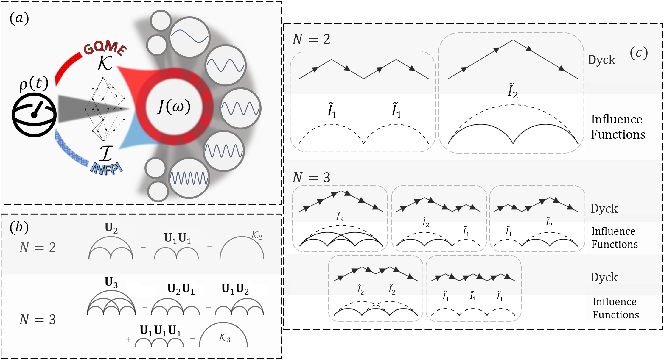
In this Article, we present a unifying description of these non-Markovian quantum dynamics frameworks. In particular, we establish explicit analytic correspondence between and . We present a visual schematic describing the main idea of our work in Fig.1 panel (a).
Path Integral Formulation.
We consider a system described by the Hamiltonian coupled to a bath that is described by a bosonic quadratic Hamiltonian, .
For simplicity, we limit our discussion to a linear system-bath coupling,
where is a system operator that is diagonal in the computational basis and is a bath operator that is linear in the bath creation and annihilation operators.
The total Hamiltonian is therefore , governing the time evolution of the full system, .
We discretize time and employ a Trotterized propagator,
(1)
where .
The initial total density matrix is assumed to be factorized into
at inverse temperature where .
Then, one can show that the dynamics of the reduced system density matrix, , follows
(2)
where .
From this, we can show that the influence functional, , is pairwise separable,
(3)
where the influence functions are defined in Appendix A, and are related to the bath spectral density, .
For later use, we note that
Eq.2 can be simplified into
(4)
where is the system propagator
from to .
It is then straightforward to express in terms of . Makri (2021a, 2020); Kundu and Makri (2023); Wang and Cai (2022)
The Nakajima-Zwanzig Equation. The Nakajima-Zwanzig equation is a time-non-local formulation of the formally exact GQME. Assuming the time-independence of , the discretized homogeneous Nakajima-Zwanzig equation takes the form
(5)
where
with
being the bare system Liouvillian and is the discrete-time memory kernel at timestep . To relate to , we inspect the reduced dynamics evolution operator as defined in Eq.4,
(6)
With this relation, one can obtain from the reduced propagators . We observe setting yields
, since is the identity.
The memory kernel, , accounts for
the deviation of the system dynamics from its pure dynamics (decoupled from the bath) within a time step.
From setting , we get
.
This intuitively shows that captures the effect of the bath that cannot be captured within .
Similarly, for ,
This set of equations
shows similarity to
cumulant expansions widely used in the context of
many-body physics and electronic structure theory.Mahan (2000); Kutzelnigg and Mukherjee (1999)
Instead of dealing with higher-order -body expectation values,
we deal with higher-order -time memory kernel in this context.
The -time memory kernel is the -th order cumulant in the cumulant expansion of the system operator.
Unsurprisingly, these recursive relations lead to
diagrammatic expansions commonly found in cumulant expansionsMahan (2000)
as shown in Fig.1 panel (b).
Figure 1: Unification of open quantum dynamics framework. Panel (a): An open quantum system, where the environment is characterized by the spectral density , can be described with the Generalized Quantum Master Equation (GQME) and the Influence Functional Path Integral (INFPI). The former distills environmental correlations through the memory kernels while the latter through the influence functionals . In this work, we show both are related through Dyck Paths, and that furthermore we can use the Dyck construction for extracting by simply knowing how the quantum system evolves. Panel (b): Cumulant expansion of memory kernel. Examples through Eq. (6) for and . Solid arcs of diameter filled with all possible arcs of diameters smaller than denote propagator . Panel (c): Dyck path diagrams. Examples for and and their corresponding influence function diagrams, which composes and respectively. Solid lines denote influence functions and dashed line denote .
Main results. Using this cumulant generation of and by expressing in terms of , we obtain a direct relationship between and . Specifically, we have
(7)
(8)
(9)
(10)
where
we define (bold-face for denoting matrices)
and . In Appendix B, we present a general algorithm for calculating higher-order memory kernels, which is critical due to their nontrivial structure when expressed in terms of and .
This series of equations is the main result of this work, showing explicitly how is constructed in terms of influence functions from to .
The computational effort of computing can be easily seen from this construction.
We sum over an additional time index for each time step.
This gives a computational cost that scales exponentially in time,
where is the dimension of the system Hilbert space.
It can be inferred from Eqs.8, 9 and 10 that each term in is represented uniquely by each Dyck path Brualdi (2010); Stanley (2015); cat (2010) of order . Hence, one can construct by generating the respective set of Dyck paths and associating each path with a tensor contraction of influence functions. This is illustrated in Fig. 1 panel (c) and further detailed in Appendix B.
This observation reveals some new properties of . First, the number of terms in is given by the -th Catalan’s numberStanley (2015); cat (2010) (i.e., has 14 such terms, has 42, then 132, 429, 1430, 4862, 16796, 58786, ). We note that Catalan’s number appeared in Ref. 45 when analyzing an approximate numerical INFPI method.
See Appendix B for more information.
Scrutinizing the relationship of and , presented in Appendix B, further, we can observe how decays asymptotically.
As is well-known, for typical condensed phase systems for .Makri and Makarov (1995b, a)
Similarly, because for large , those terms with larger multiplicities contribute less to and decay exponentially to zero as multiplicity grows.
In fact, for condensed phase systems, the decay of and is often rapid, which motivated the development of approximate INFPI methodsMakri and Makarov (1995b, a); Makarov and Makri (1994); Makri (2021a, 2020) and other approximate GQME methods.Montoya-Castillo and Reichman (2016); Mulvihill and Geva (2021b); Mulvihill et al. (2019); Kelly et al. (2016)
With our new insight, one can look at approximate INFPI methods through the lens of the corresponding memory kernel content (and vice versa).
As an example, we shall discuss the iterative quasiadiabatic path-integral methods.Makri and Makarov (1995b, a); Makarov and Makri (1994) In these methods, is set to unity beyond a preset truncation length . For simplicity, let us consider , and hence and for . We now inspect what this approximation entails for . First, no approximation is applied to and . Then, in (Eq.9),
(11)
Similarly, in (Eq.10), the only surviving contribution is from .
We hope such a direct connection between approximate methods will inspire the development of more efficient and accurate methods.
The time-translational structure of the INFPI formulation and its Dyck-diagrammatic structure allow for a recursive deduction of from , which is the inverse map of Eqs.8, 9 and 10.
We first observe that
(12)
where we obtained from .
One can then show that
(13)
using and .
Similarly, inspecting the expression for gives us
(14)
where as well as are obtained from the previous two relations.
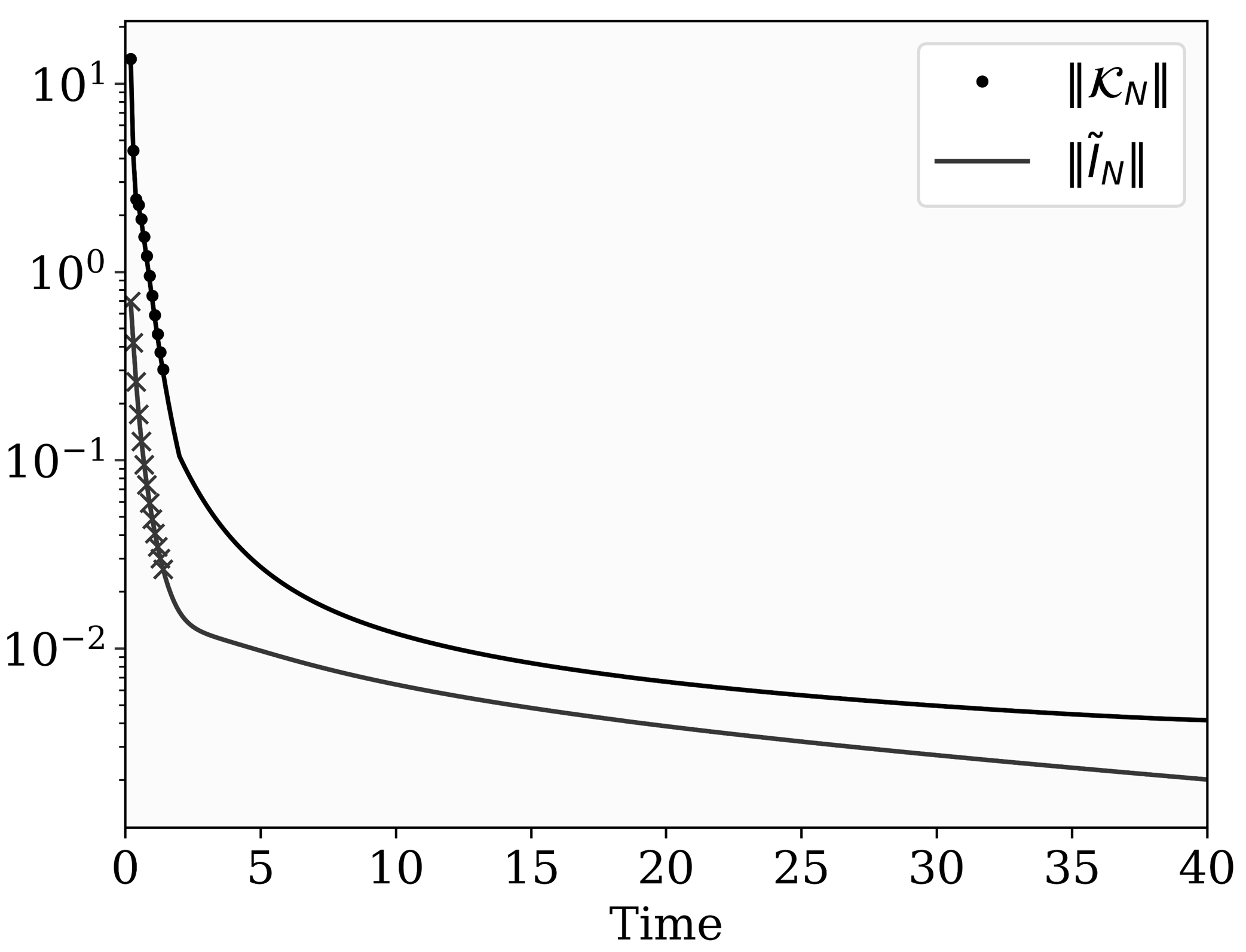
Figure 2: Verification of the Dyck construction.
Operator norm of (Light) and (Dark) as a function of .
Lines denote computed from analytic expressions and from post-processing exact numerical results via the transfer tensor method.Cerrillo and Cao (2014) Circles denote from the Dyck diagrammatic method, and crosses are obtained via the inverse map discussed in Eqs.13 and 14. Dashed lines denote the operator norm of the crest term of (the Dyck path diagram with the highest height). Parameters used are: (other parameters are expressed relative to ), , , , , and and (panel (a)),
In Appendix C, we present a general recursive procedure using the Dyck paths and how to obtain the bath spectral density from . As a result, we achieve the following mapping from left to right,
(15)
A remarkable outcome of this analysis is that one can completely characterize the environment (i.e., ), by inspecting the reduced system dynamics.
Such a tool is powerful in engineering quantum systems in experiments where we have access to only the reduced system Hamiltonian and reduced system dynamics, but lack information about the environment. Furthermore, this approach provides an alternative to quantum noise spectroscopyDegen et al. (2017); Sung et al. (2021).
This type of Hamiltonian learning with access only to subsystem observables has been achieved for other simpler Hamiltonians,Burgarth et al. (2011); Di Franco et al. (2009) but to our knowledge, for the Hamiltonian considered here, our work is the first to show this inverse map.
Note that the expression Eq.13 can become ill-defined when is diagonal.
This occurs when is diagonal and commutes with , constituting a purely dephasing dynamics. In that case, the reduced system dynamics is governed only by the diagonal elements of , and similarly is diagonal, as clearly seen in our Dyck path construction.
As a result, the map is no longer bijective in that we cannot obtain off-diagonal elements of . Regardless, one can still extract using only the diagonal elements of via inverse cosine transform (see Appendix C). One may worry Eq.14 could also become ill-conditioned when its denominator vanishes, but is not diagonal. If that were the case, the propagator would become zero. Therefore, this condition cannot be satisfied in general.
Generalization to Driven Systems. While analysis up to this point considered general time-independent systems, in many scenarios, e.g., of biological or engineering relevance, particularly for quantum control applicationsMa et al. (2021), a time-dependent description of the system is necessary.
In such cases, loses its time-translational properties and should depend on two times. Consequently, Eq.6 cannot be applied. To overcome this, we factorize into time-dependent and time-independent parts (see Appendix D for more details). This can be achieved straightforwardly,
as follows: one observes upon the inclusion of time-dependence in , the terms that are affected in , Eqs.7, 8, 9 and 10, are only the bare system propagators and .
We define the remainder as tensors with number of indices, , which includes all the influence of the bath between time steps. These tensors only need to be computed once and reused for a later time. Then, one builds the kernels via tensor contraction over two tensors,
(16)
where denotes indices, , and the tensor encapsulates the time-dependence of the system Hamiltonian and is constructed only out of bare system propagators.
The tensor, , then consists only of influence functions, up to .
The construction of these tensors is straightforward with following the Dyck path construction presented for time-independent system dynamics.
Some relevant numerical results for open, driven system dynamics are presented in Appendix D.
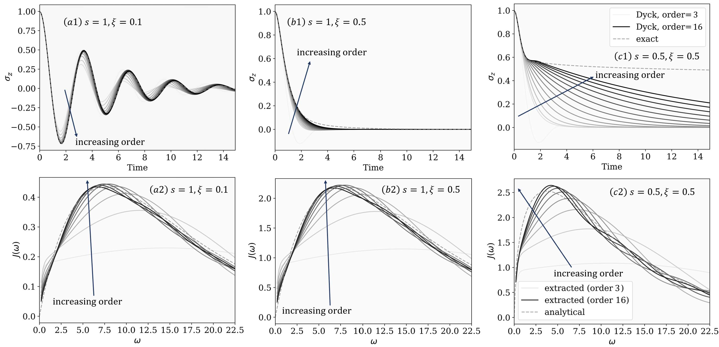
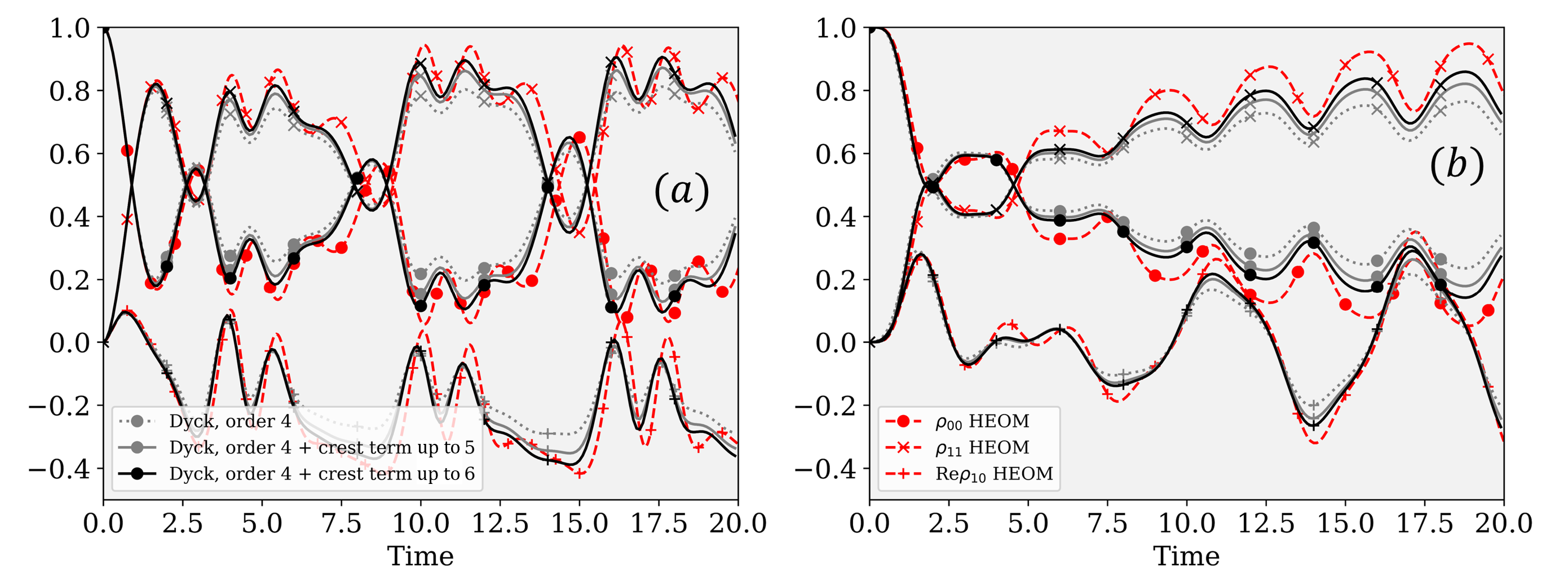
Figure 3: Dynamics of spin-boson model with truncated Dyck paths. Panels (a1), (b1), and (c1): Magnetization () dynamics predicted using constructed via Dyck diagrams with increasing truncation orders (from light to darker colors) compared to exact results (see Appendix F). Panels (a2), (b2), and (c2): Bath spectral densities extracted through the Dyck diagrammatic method with increasing truncation order (from white to black colors) compared to exact spectral densities (dashed), see Appendix C for more details. These results come from numerically exact trajectories, initiated from linearly independent initial states .
Parameters used are: (other parameters are expressed relative to ), , , (panels (a1), (b1), and (c1)) or (Panels (a2), (b2), and (c2)), , and and (panels (a1) and (a2)),
and (panels (b1) and (b2)), or and (panels (c1) and (c2)).
Numerical results. The spin-boson model is an archetypal model for studying open quantum systems.Leggett et al. (1987) The model comprises a two-level system coupled linearly to a bath of harmonic oscillators. Hence, it and its generalizations have been used to understand various quantum phenomena: transport, chemical reactions, diode effect, and phase transitions.Nitzan (2006)
While the construction of discussed above is applicable to a generic system linearly coupled to a harmonic bath, we numerically verify our findings within the spin-boson model. Specifically,
we now use , coupled via to a harmonic bath with spectral density () Leggett et al. (1987)
(17)
where , is the Kondo parameter, and is the Ohmicity. All reference calculations were performed using the HEOM method.Tanimura and Kubo (1989); Tanimura (2020b); Xu et al. (2022) Details of the HEOM implementation used here are provided in Appendix E.
In Fig.2, we investigate a series of spin-boson models corresponding to weak and intermediate coupling to an Ohmic environment () as well as strong coupling to a subohmic environment (). In panels (a) and (b), we observe that the decay of is rapid for the Ohmic cases. This translates to a similarly rapid decay for the respective , although one can see that both and are overall scaled larger in the strong coupling regime. This is to be contrasted with the results for the strongly coupled subohmic environment shown in panel (c).
The decay of the is slow, accompanied by a similarly slow decay of .
Interestingly, the rates by which both and decay are similar.
We also see perfect agreement between constructed from our Dyck diagrammatic method and those obtained by numerically post-processing exact trajectories via the transfer tensor method. Cerrillo and Cao (2014) Lastly, we construct from up to as exemplified in Eqs.13 and 14 and observe perfect agreement between our and those computed from its known analytic formula.
We note that the term with (multiplicity of 1) contributes the most to the memory kernel, for all parameters considered in our work.
We refer to this term as the “crest” term, which corresponds to the Dyck path that goes straight to the top and down straight to the bottom, having the tallest height.
We see a small difference between the crest term norm and the full memory kernel norm in Fig.2, indicating that the memory kernel is dominated by the crest term.
Since the decay of is directly related to the decay of the bath correlation function, one can also make connections between the memory kernel decay and the bath correlation function decay.
Nonetheless, for a stronger system-bath coupling (e.g., Fig.2 (b)) and for cases
with a long-lived memory (e.g., Fig.2 (c)), terms other than the crest term contribute non-negligibly, making general analysis of the memory kernel decay challenging.
The cost to numerically compute scales exponentially with . Nevertheless, it is possible to exploit the decay of , which is rapid for some environments, e.g., ohmic baths, in turn signifying the decay behavior of . This allows truncating the summation in Eq. (5), enabling dynamical propagation to long times (with linear costs in time) as usually done in small matrix path integral methods Makri (2021a, 2020) and GQMECerrillo and Cao (2014) methods. We show in panels (a1) and (b1) of Fig. (3) that this procedure applied to a problem with a rapidly decaying quickly converges to the exact value with a reasonably low-order.
On the other hand, for environments with slowly decaying , the truncation scheme struggles to work effectively. For a strongly coupled subohmic environment, as shown in Fig. (3) panel (c1), one would need truncation orders beyond current computational capabilities (of about 16) to converge to the exact value. Nonetheless, this illustrates that our direct construction of can recover exact dynamics if sufficiently high-order is used. Furthermore, the construction is non-perturbative and can be applied to strong coupling problems.
Finally, in Fig. (3) panels (a2), (b2), and (c2), we show the extraction of spectral densities for three distinct environments. The extracted converges to the analytical value as we obtain the influence functions to higher orders.
This shows that we can indeed invert the reduced system dynamics to obtain given the knowledge of the system Hamiltonian, which ultimately characterizes the entire system-bath Hamiltonian.
Nonetheless, the accuracy of the resulting depends on the highest order of we can numerically extract. The cost of extracting scales exponentially in without approximations, so there is naturally a limit to the precision of in practice.
Furthermore, we show how this procedure can extract highly structured spectral densities as well in SectionAppendix F and Fig.11. New opportunities await in using approximately inverted and quantifying the error in the resulting .
Conclusion. In this Article, we provide analytical analysis and numerical evidence that show complete equivalence between the memory kernel () in the GQME formalism and the influence function () used in INFPI. Our analysis is applicable to a general (driven) system interacting with a harmonic bath via linear coupling.
Furthermore, we presented a general, non-perturbative algorithm based on a diagrammatic analysis to construct exactly from the influence functions. Unlike available approaches, our direct construction of does not require any projection-free trajectories input. Furthermore, we showed that one can extract the bath spectral density from the reduced system dynamics with the knowledge of the reduced system Hamiltonian .
We believe that this unified framework for studying non-Markovian dynamics will facilitate the development of new analytical and numerical methods that combine the strengths of both GQME and INFPI.
Acknowledgements. F.I. and J.L. were supported by Harvard University’s startup funds. L.P.L acknowledges the support of the Engineering and Physical Sciences
Research Council [grant EP/Y005090/1]. We thank Nathan Ng, David Reichman, Dvira Segal, and Jonathan Keeling for stimulating discussions, Tom O’Brien for discussions on Hamiltonian learning, and Hieu Dinh for providing a code to generate the Dyck path. Computations were carried out partly on the FASRC cluster supported by the FAS Division of Science Research Computing Group at Harvard University. This work also used the Delta system at the National Center for Supercomputing Applications through allocation CHE230078 from the Advanced Cyberinfrastructure Coordination Ecosystem: Services & Support (ACCESS) program, which is supported by National Science Foundation grants #2138259, #2138286, #2138307, #2137603, and #2138296.
References
Breuer and Petruccione (2002)
H.-P. Breuer and F. Petruccione, The theory of open quantum systems (Oxford University Press, USA, 2002).
Gröblacher et al. (2015)
S. Gröblacher, A. Trubarov, N. Prigge, G. D. Cole, M. Aspelmeyer, and J. Eisert, Nature Communications 6, 7606 (2015), ISSN 2041-1723, URL https://doi.org/10.1038/ncomms8606.
Chin et al. (2012)
A. W. Chin, S. F. Huelga, and M. B. Plenio, Philosophical Transactions of the Royal Society A: Mathematical, Physical and Engineering Sciences 370, 3638 (2012).
Ishizaki and Fleming (2009)
A. Ishizaki and G. R. Fleming, The Journal of Chemical Physics 130, 234111 (2009), ISSN 0021-9606, eprint https://pubs.aip.org/aip/jcp/article-pdf/doi/10.1063/1.3155372/13131430/234111_1_online.pdf, URL https://doi.org/10.1063/1.3155372.
Andersson et al. (2019)
G. Andersson, B. Suri, L. Guo, T. Aref, and P. Delsing, Nature Physics 15, 1123 (2019), ISSN 1745-2481, URL https://doi.org/10.1038/s41567-019-0605-6.
Bylicka et al. (2014)
B. Bylicka, D. Chruściński, and S. Maniscalco, Scientific Reports 4, 5720 (2014), ISSN 2045-2322, URL https://doi.org/10.1038/srep05720.
Bylicka et al. (2013)
B. Bylicka, D. Chruściński, and S. Maniscalco, Non-markovianity as a resource for quantum technologies (2013), eprint 1301.2585.
Tanimura (2020a)
Y. Tanimura, J. Chem. Phys. 153 (2020a), ISSN 0021-9606.
Strathearn et al. (2018)
A. Strathearn, P. Kirton, D. Kilda, J. Keeling, and B. W. Lovett, Nature Communications 9, 3322 (2018), ISSN 2041-1723, URL https://doi.org/10.1038/s41467-018-05617-3.
Makri and Makarov (1995a)
N. Makri and D. E. Makarov, The Journal of Chemical Physics 102, 4611 (1995a).
Makarov and Makri (1994)
D. E. Makarov and N. Makri, Chemical Physics Letters 221, 482 (1994).
Makri (2021a)
N. Makri, Journal of Chemical Theory and Computation 17, 1 (2021a).
Makri (2020)
N. Makri, The Journal of Chemical Physics 152, 041104 (2020).
Kundu and Makri (2023)
S. Kundu and N. Makri, The Journal of Chemical Physics 158, 224801 (2023), ISSN 0021-9606, eprint https://pubs.aip.org/aip/jcp/article-pdf/doi/10.1063/5.0151748/17987394/224801_1_5.0151748.pdf, URL https://doi.org/10.1063/5.0151748.
Kilgour et al. (2019)
M. Kilgour, B. K. Agarwalla, and D. Segal, The Journal of Chemical Physics 150, 084111 (2019), ISSN 0021-9606, URL https://doi.org/10.1063/1.5084949.
Simine and Segal (2013)
L. Simine and D. Segal, The Journal of Chemical Physics 138, 214111 (2013), ISSN 0021-9606, URL https://doi.org/10.1063/1.4808108.
Makri (2018)
N. Makri, The Journal of Chemical Physics 149, 214108 (2018), ISSN 0021-9606, eprint https://pubs.aip.org/aip/jcp/article-pdf/doi/10.1063/1.5058223/15551048/214108_1_online.pdf, URL https://doi.org/10.1063/1.5058223.
Lambert and Makri (2012)
R. Lambert and N. Makri, The Journal of Chemical Physics 137, 22A552 (2012), ISSN 0021-9606, eprint https://pubs.aip.org/aip/jcp/article-pdf/doi/10.1063/1.4767931/14007017/22a552_1_online.pdf, URL https://doi.org/10.1063/1.4767931.
Tanimura (2006)
Y. Tanimura, Journal of the Physical Society of Japan 75, 082001 (2006), eprint https://doi.org/10.1143/JPSJ.75.082001, URL https://doi.org/10.1143/JPSJ.75.082001.
Link et al. (2023)
V. Link, H.-H. Tu, and W. T. Strunz, arXiv (2023), eprint 2307.01802.
Gribben et al. (2022)
D. Gribben, D. M. Rouse, J. Iles-Smith, A. Strathearn, H. Maguire, P. Kirton, A. Nazir, E. M. Gauger, and B. W. Lovett, PRX Quantum 3, 010321 (2022), URL https://link.aps.org/doi/10.1103/PRXQuantum.3.010321.
Breuer and Petruccione (2007)
H.-P. Breuer and F. Petruccione, The Theory of Open Quantum Systems (Oxford University Press, 2007), ISBN 0199213909.
Kidon et al. (2018)
L. Kidon, H. Wang, M. Thoss, and E. Rabani, J. Chem. Phys. 149 (2018), ISSN 0021-9606.
Cohen and Rabani (2011)
G. Cohen and E. Rabani, Phys. Rev. B 84, 075150 (2011).
Mühlbacher and Rabani (2008)
L. Mühlbacher and E. Rabani, Phys. Rev. Lett. 100, 176403 (2008).
Wang and Cai (2022)
G. Wang and Z. Cai, Tree-based implementation of the small matrix path integral for system-bath dynamics (2022), eprint 2207.11830.
Mahan (2000)
G. D. Mahan, Many-particle physics (Springer Science & Business Media, 2000).
Kutzelnigg and Mukherjee (1999)
W. Kutzelnigg and D. Mukherjee, J. Chem. Phys. 110, 2800 (1999), ISSN 0021-9606.
Makri and Makarov (1995b)
N. Makri and D. E. Makarov, The Journal of Chemical Physics 102, 4600 (1995b).
Montoya-Castillo and Reichman (2016)
A. Montoya-Castillo and D. R. Reichman, The Journal of Chemical Physics 144, 184104 (2016), ISSN 0021-9606, eprint https://pubs.aip.org/aip/jcp/article-pdf/doi/10.1063/1.4948408/13820400/184104_1_online.pdf, URL https://doi.org/10.1063/1.4948408.
Mulvihill and Geva (2021b)
E. Mulvihill and E. Geva, The Journal of Physical Chemistry B 125, 9834 (2021b), ISSN 1520-6106, publisher: American Chemical Society, URL https://doi.org/10.1021/acs.jpcb.1c05719.
Mulvihill et al. (2019)
E. Mulvihill, X. Gao, Y. Liu, A. Schubert, B. D. Dunietz, and E. Geva, The Journal of Chemical Physics 151, 074103 (2019), ISSN 0021-9606, eprint https://pubs.aip.org/aip/jcp/article-pdf/doi/10.1063/1.5110891/15562688/074103_1_online.pdf, URL https://doi.org/10.1063/1.5110891.
Kelly et al. (2016)
A. Kelly, A. Montoya-Castillo, L. Wang, and T. E. Markland, J. Chem. Phys. 144 (2016), ISSN 0021-9606.
Sung et al. (2021)
Y. Sung, A. Vepsäläinen, J. Braumüller, F. Yan, J. I.-J. Wang, M. Kjaergaard, R. Winik, P. Krantz, A. Bengtsson, A. J. Melville, et al., Nature communications 12, 967 (2021).
Burgarth et al. (2011)
D. Burgarth, K. Maruyama, and F. Nori, New J. Phys. 13, 013019 (2011), ISSN 1367-2630.
Di Franco et al. (2009)
C. Di Franco, M. Paternostro, and M. S. Kim, Phys. Rev. Lett. 102, 187203 (2009).
Leggett et al. (1987)
A. J. Leggett, S. Chakravarty, A. T. Dorsey, M. P. A. Fisher, A. Garg, and W. Zwerger, Rev. Mod. Phys. 59, 1 (1987), URL https://link.aps.org/doi/10.1103/RevModPhys.59.1.
Nitzan (2006)
A. Nitzan, Chemical Dynamics in Condensed Phases: Relaxation, Transfer, and Reactions in Condensed Molecular Systems (New York: Oxford University Press, 2006).
Tanimura and Kubo (1989)
Y. Tanimura and R. Kubo, J. Phys. Soc. Jpn. 58, 101 (1989).
Tanimura (2020b)
Y. Tanimura, J. Chem. Phys. 153, 020901 (2020b).
Bernini et al. (2007)
A. Bernini, I. Fanti, and E. Grazzini, An exhaustive generation algorithm for catalan objects and others (2007), eprint math/0612127.
Neri (2018)
C. Neri, A loopless and branchless algorithm to generate the next dyck word (2018), eprint 1602.06426.
OEIS Foundation Inc. (2023)
OEIS Foundation Inc., The On-Line Encyclopedia of Integer Sequences (2023), published electronically at http://oeis.org.
Makri (2021b)
N. Makri, The Journal of Physical Chemistry A 125, 10500 (2021b), pMID: 34812645, eprint https://doi.org/10.1021/acs.jpca.1c08230, URL https://doi.org/10.1021/acs.jpca.1c08230.
Nakatsukasa et al. (2018)
Y. Nakatsukasa, O. Sète, and L. N. Trefethen, SIAM Journal on Scientific Computing 40, A1494 (2018), eprint https://doi.org/10.1137/16M1106122, URL https://doi.org/10.1137/16M1106122.
Shi et al. (2018)
Q. Shi, Y. Xu, Y. Yan, and M. Xu, The Journal of Chemical Physics 148, 174102 (2018), ISSN 0021-9606, eprint https://pubs.aip.org/aip/jcp/article-pdf/doi/10.1063/1.5026753/15539991/174102_1_online.pdf, URL https://doi.org/10.1063/1.5026753.
Mangaud et al. (2023)
E. Mangaud, A. Jaouadi, A. Chin, and M. Desouter-Lecomte, The European Physical Journal Special Topics 232, 1847 (2023), ISSN 1951-6401, URL https://doi.org/10.1140/epjs/s11734-023-00919-0.
Ke (2023)
Y. Ke, The Journal of Chemical Physics 158, 211102 (2023), ISSN 0021-9606, eprint https://pubs.aip.org/aip/jcp/article-pdf/doi/10.1063/5.0153870/18143581/211102_1_5.0153870.pdf, URL https://doi.org/10.1063/5.0153870.
We present a more detailed formulation of the influence-functional-based path-integral (INFPI) approaches.
We consider the general Hamiltonian of a quantum system interacting with external degrees of freedom,
(A1)
where is the system Hamiltonian, , and
where is a system operator and .
The time evolution of the density matrix of the full system, (pure state for simplicity, further assumed separable ) follows
(A2)
With the quasiadiabatic approximation, one may split the total Hamiltonian as (here )
(A3)
With this identity we express the trotterized evolution as (summation over the paths implied)
(A4)
We work in the diagonal basis (note for some system operator and bath operator ) and insert resolution-of-the-identity in between every and to obtain
(A5)
Since
(A6)
we therefore have
(A7)
where .
When the density matrix is separable (as assumed earlier) and where is quadratic in bath operators (as we have and as assumed commonly) the influence functionals take a pairwise product form as shown in Eq.3.
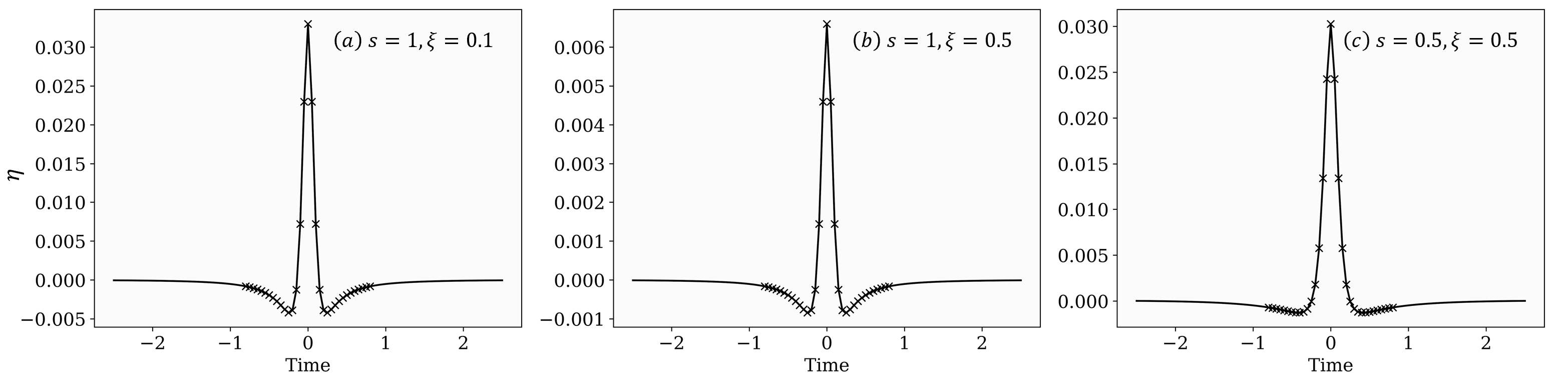
For , influence functions are given as
(A8)
where
(A9)
(A10)
We recall that
(A11)
Note that we can recover Eq. (A10) from Eq. (A9) by using which is a purely imaginary and odd function.
If one writes the propagators in a more compact form (for )
(A12)
the auxiliary propagators can be written as
(A13)
(A14)
(A15)
where the underbraced terms and the last line is analogous to the memory matrix in small matrix path integral (SMatPI) methods Makri (2021a, 2020); Kundu and Makri (2023) and the transfer tensors in the transfer tensor method (TTM)Cerrillo and Cao (2014), both of which can be cast into the memory kernels . However, crucial differences emerge here which makes Eqs. (A13) - (A15) distinct and cannot be obtained from SMatPI or TTM: (1) Here they are completely time-translationally invariant, while in SMatPI they are not, (2) Here and therefore the analysis of TTM is not applicable.
One may proceed as in the main text to recover the memory kernels from the propagators.
Appendix A.2 Explicit Correspondence with GQME
The Nakajima-Zwanzig (NZ) equation takes the form
(A16)
In this work, the inhomogeneous term vanishes due to the factorized initial condition assumption . The discretized form of the homogeneous NZ equation is
(with )
(A17)
By noting that (where ) we get
(A18)
We then obtain in terms of by matching each multiplier of recursively. For example, for ,
(A19)
so
(A20)
that is,
(A21)
For ,
(A22)
One observes that with the time-translational invariance of the memory kernels (i.e., valid if the system Hamiltonian does not have explicit time-dependence),
(A23)
We use this and make appropriate substitutions in our previous results.
Then, we obtain
(A24)
Hence,
(A25)
Similarly, for ,
(A26)
One observes many terms again cancel, leaving
(A27)
Making appropriate substitutions into , , and ,
(A28)
We again factorize as follows
(A29)
The underbraced terms cancel with the first three terms in Eq. (A28) and we are left with
(A30)
For ,
(A31)
So,
(A32)
We factorize as follows
(A33)
For now notice that
(A34)
because
(A35)
note there
(A36)
and also that
(A37)
These resulting identities then group terms in Eq. (A32) to give Eq. (10) in the main text.
Now for (we use ):
(A38)
Evidently, the number of terms grows combinatorially with the number of timesteps . In the next section, we devise a general scheme to build memory kernels at arbitrary time based on Dyck diagrams.
Appendix B Nakajima-Zwanzig Dyck-Diagrammatic Formalism
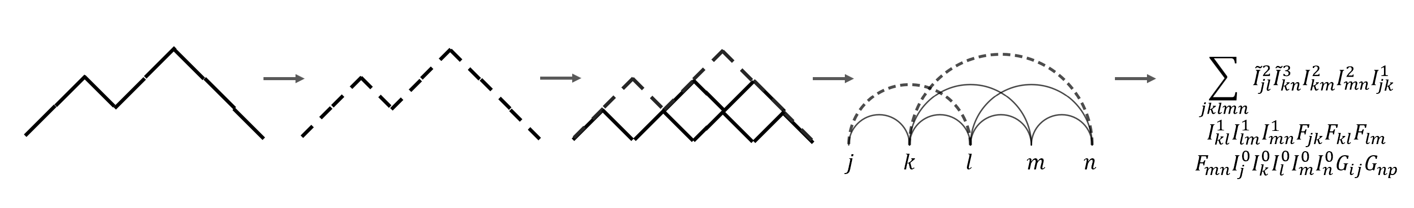
The structure of terms in via the decomposition through has the following properties. The number of terms in is given by Catalan’s numbersStanley (2015); cat (2010) , as was pointed out in Ref. 45. More importantly, the terms in are given by Dyck path diagrams Stanley (2015); cat (2010) (of which there are paths). A Dyck path is a sequence of up-steps and down-steps that start and end on the -axis but never go below. The order of a Dyck path is given by the number of up-steps, which must equal the number of down-steps. The study of Dyck paths is at the root of combinatorial mathematicsVilenkin (1971), and algorithms already exist to generate all Dyck paths of any order.Bernini et al. (2007); Neri (2018)
Alternatively, one can also generate all (sometimes also called k-tuples) possible permutations (repetitions allowed, since here accounting for up or down steps we then have , and so on) of and and then filter (i.e., such path must have equal amounts of and and furthermore at any point the path must not go below the -axis and so on) for an order Dyck path. To obtain the terms in from a particular Dyck path, we map a Dyck path into an influence functional diagram based on the following rules:
1.
The Dyck path is made dashed.
2.
Now one draws all possible triangles in each segment of a Dyck path, but none could be as tall as any dashed peak. This step is drawn in solid. A segment of a Dyck path is defined as the sub-path of a Dyck path which starts and ends at (the full path itself is not counted). A peak is defined as the point at which an up-step meets a down-step, in that order.
3.
If any dashed down path sequence does not reach , one continues to draw it until it does, this is with dashed lines.
4.
One rounds the vertices.
5.
Dashed correlations connecting points and are , while solid correlations are . Further terms can be read immediately from the diagrams.
An example of this algorithm is shown in Fig. (4).
Figure 4: Visual schematic of the algorithm to convert Dyck diagrams into terms in .
We furthermore enumerate some properties of Dyck paths, which therefore unveils the general properties of :
1.
The set of all Dyck paths of order has Narayana’s number, , the number of paths with peaks. The number of peaks is the multiplicity of in the term. is given by
(A39)
It is not difficult to show that .
2.
The number of Dyck paths in the set of all Dyck paths of order having number of segments is given by Catalan’s triangle :
(A40)
In particular, if , is the th Catalan’s number .
3.
The number of Dyck paths in the set of all Dyck paths of order having no hills (a segment of height ), that is those with no term, is given by the Fine numbers with generating function Deutsch and Shapiro (2001):
(A41)
This distribution also describes (1) Dyck paths where the leftmost peak is of even height,Deutsch and Shapiro (2001) and (2) the number of even returns to the horizontal axis (valley of height 0)Deutsch and Shapiro (2001).
4.
The number of Dyck paths in the set of all Dyck paths of order with returns to the horizontal axis is given by the Ballot numbers
(A42)
5.
The number of Dyck paths in the set of all Dyck paths of order with
occurrences of different is given by , where is related to Motzkin’s number viaSun (2004)
(A43)
Particularly, the generator of Motzkin’s number , , satisfies
(A44)
6.
The number of Dyck paths in the set of all Dyck paths of order whose peaks’ height total to can be read off from Triangle A094449.OEIS Foundation Inc. (2023)
Further properties of the Dyck paths have been enumerated in great detail in the On-Line Encyclopedia of Integer SequencesOEIS Foundation Inc. (2023).
To construct the memory kernels via this approach, we can represent Dyck paths as Dyck Words. becomes and becomes . Hence, the Dyck path in Fig. (4) is .
By representing each path by a bit string, we can write an efficient code that enumerates all possible Dyck paths of order . The conversion code is available upon request.
Appendix C Details on Computing from
We provide more details on the inverse extraction procedure that goes from reduced system dynamics, , to the bath spectral density, . We show that such a map is nearly bijective in that any aspects of that affect the reduced system dynamics can be obtained by analyzing . This construction has a direct connection with Hamiltonian learning literature, as pointed out in our main text.
To proceed, we recall
(A45)
We will explain step-by-step how to go from left to right.
First, to obtain from note that , where is a vector in Liouville space with a dimension of . is then a matrix. With linearly-independent trajectories (obtained experimentally or computationally), we can uniquely determine . We then stack them to make the matrix
(A46)
With this definition, we arrive at a simple linear equation to solve,
(A47)
By inverting , we obtain
(A48)
is invertible because each trajectory is generated from a linearly independent initial condition.
While we only considered noise-free data inputs, if the data is noisy, one can use more trajectories than (i.e., and become a fat matrix) and perform the Moore-Penrose pseudoinverse, which could help mitigate noise.
To obtain from we decompose the latter iteratively, in the manner presented in the main text Eq. (6) and e.g., Ref. 41.
Next, we move to obtain from . First, we define which is defined through .
From , we have
(A49)
Similarly, we have
(A50)
For , we have
(A51)
which leads to
(A52)
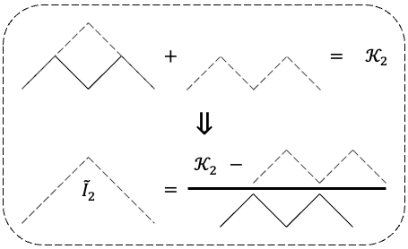
This procedure is, in fact, diagrammatically generalizable–its diagrammatic equation is shown in Fig. (5). One can generate all Dyck diagrams (which can be translated into a particular term in ) of order . From the sum of all diagrams, one moves all diagrams except the crest term to the side of . The crest term corresponds to the diagram that contains . Then, one divides both sides of the equation with the rest of the terms, which then yields .
Figure 5: Visual schematic of the inversion diagram for
Now to obtain from , we start by taking the logarithm of Eq.A8,
(A53)
Here, we consider the spin-boson model with coupling, so . In this example, we have
(A54)
(A55)
We can also readily obtain from through a similar manner.
Lastly, to obtain the spectral density, , we recall that (for clarity )
(A56)
where
(A57)
Note, in practice, we construct from for and take the hermitian conjugate of for . We use for .
To extract with the knowledge of we perform a Fourier Transform
(A58)
which, in practice, is performed via a discrete Fourier transform
(A59)
This immediately gives the spectral density through
(A60)
One must pay special attention to frequencies with for integer as the denominator in Eq.A60 is zero. This is not a problem because the spectral density at such values does not alter the reduced system dynamics as they do not contribute to as shown in Eq.A59.
Another case to consider is the pure dephasing limit where is diagonal and commutes with .
In this case, only the real part of is available,
(A61)
We can then perform the inverse cosine transform to obtain ,
(A62)
Appendix D The Driven Open Quantum System
Here, we consider the explicit time dependence in the system Hamiltonian. We start by inspecting the INFPI formalism without assuming any time-translational invariance of any tensors:
(A63)
with . There, is the system Hamiltonian at time . Hence,
(A64)
(A65)
Similarly, the memory kernels are no longer time-translationally invariant. Consider
(A66)
(A67)
where with
. We also have
(A68)
Hence,
(A69)
This allows us to write in terms of :
(A70)
Inspecting equations for later time , we observed that the structure of the remains largely unchanged except for including time indices for the bare system propagators. In particular, we collect all the terms except the time-dependent ones (only the bare system propagators) as a tensor, which is time-translational. That is,
(A71)
(A72)
where , .
Figure 6: Dynamics of various driven systems open to a thermal bosonic environment.
Parameters used are: (other parameters are expressed relative to ), , , , and .
The memory kernel is truncated at the th timestep for the
Dyck diagrammatic method (dashed) with an additional leading term correction, the diagrams with the highest heights (smallest multiplicity), upto the sixth timestep (solid)
These trajectories are compared to the exact HEOM results.
For problems with driven Hamiltonians, methods relying on time-translational invariance of memory kernels such as TTM become inapplicable to apply since the transfer tensor depends explicitly on time. Other schemes that treat this problemMakri (2021b); Kundu and Makri (2023) seem limited to invoking periodicity and temporal symmetries at least in terms of numerical efficiency. Here, we devise an efficient procedure to perform reduced system dynamics, exploiting the time-translational symmetry of the s. The plan goes as follows: One computes all the up until a predefined truncation parameter . Then, to obtain the kernel at time one performs a tensor contraction with the time-dependent bare system propagator tensor, which is trivial to obtain.
As a proof of concept, we consider various driven systems in Fig. (6), where in panel (a): , and in
panel (b): . In these results, we include all Dyck diagrams up to the fourth order to compute to . We then approximate and by including only the diagram with the smallest multiplicity (i.e., the crest term), which is justified since the coupling here is weak and so . We observe that while the order Dyck diagrammatic method captures the main features of the exactly computed driven dynamics (with HEOM), it is still not converged. After we include leading order correction terms up to 6 (including only the diagram with the highest height), we observe that the Dyck diagrammatic method converges to the exact values.
In panel (a), the diagonal elements of the Hamiltonian are driven. As expected, we see a lot of interlevel population crossing here. This is to be contrasted with panel (b), where the population of is mostly larger than except for some initial time. We also observe that for the latter, the oscillations of the populations are more regular.
Appendix E HEOM Calculations
All hierarchical equations of motion (HEOM) Tanimura and Kubo (1989); Tanimura (2020b) calculations presented in this work made use of the free pole HEOM variant,Xu et al. (2022) which makes use of the adaptive Antoulas–Anderson (AAA) algorithmNakatsukasa et al. (2018) for constructing a simple rational function approximation to the bath noise spectrum,
(A73)
which, in turn, gives rise to a sum of exponential functions representation of the bath correlation function
(A74)
with .
The HEOM approach makes use of the Feynman-Vernon influence functional discussed in Appendix A, to obtain a description of the exact dynamics of an open quantum system in terms of an infinite hierarchy of auxiliary density operators (ADOs), , that encode the system-bath correlations. These ADOs are indexed by two sets of integers and , each of length .Xu et al. (2022)
For practical calculations, this hierarchy is truncated such that no element of or is greater than some integer .
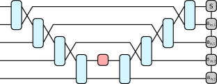
Figure 7: An illustration of a single time step of the swap based two-site TEBD algorithm used to integrate the FP-HEOMs. Crossing of lines indicates a swap operation applied to the MPS state. The grey rectangles represent the MPS representation of the hierarchy of ADOs, . The light blue rectangles correspond to the short time bath propagators, , , and red rectangles correspond to the short time system propagator term, .
Within the FP-HEOM method, this hierarchy of ADOs evolves according to the equations of motionXu et al. (2022)
(A75)
where () corresponds to the set of indices () but with the -th element incremented (+) or decremented (-) by one.
These equations have the general form
(A76)
where is an operator that acts on system and the -th mode of the hierarchy of ADOs.
For the ohmic and subohmic spectral densities with exponential cutoffs considered in this work, the total number of exponentials in the sum of exponential representation of the bath correlation function leads to a set of auxiliary density operators that are too large to represent exactly. Following references Shi et al., 2018; Xu et al., 2022; Mangaud et al., 2023 we use a matrix product state (MPS) representation of the ADOs. Evolution of the HEOMs is performed through the use of a two-site time-evolving block decimation (TEBD) algorithm that makes use of a symmetric Trotter splitting of the short-time HEOM propagator,
(A77)
In contrast to the single-site time-dependent variational principle-based schemes that have previously been used for the time evolution of tensor network-based approximations to the HEOMs,Shi et al. (2018); Lindoy (2019); Xu et al. (2022); Mangaud et al. (2023); Ke (2023) the use of a two-site TEBD scheme naturally allows for adaptive control of the MPS bond dimension throughout a simulation.
The interactions present in the HEOMs given in Eq. A75 have a star topology; terms acting on two modes of the system all act on the system degree of freedom as well as one of the modes of the hierarchy. The application of the propagator in Eq. A77 would require the application of two-body operators acting on modes that are not nearest-neighbor in the MPS, giving rise to an algorithm that requires two-site updates at each time step. To avoid this overhead, we employ a strategy where at the application of each two-body term, we swap the position of the system and bath site being acted upon, ensuring that at each stage the next two-body operator to apply is a local operation on the MPS.Bauernfeind et al. (2017); Bauernfeind (2018) This update scheme is illustrated schematically in Fig. 7, and requires two-site updates at each time step. This scheme has the advantage that at each stage, we perform a TEBD update between the system site and a single bath site. Consequentially, when the system Liouville space dimension is much smaller than the hierarchy depth, the cost of two-site updates will be dramatically reduced compared to the naive approach.
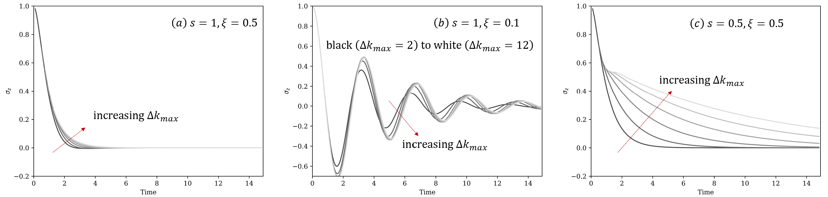
Figure 8: Magnetization () dynamics predicted using i-QuAPI method with increasing (from black to white colors, to .). Parameters used are: , , , , , and and (panel (a)),
and (panel (b)), or and (panel (c))
Appendix F Additional Simulations
For Figures (2) and (3) panels (a) and (b), the exact results from which our calculations compare come from converged HEOM results. We cross-validate these results using the i-QuAPI method, which agrees with HEOM, see Fig. (8).
Fig. (2) panel (c) suggests that the decay of (and hence ) is extremely slow. One question is if they eventually decay to zero at all. In Fig. (9) we present and for longer times than in the main text. We observe that neither has vanished and both are still decaying even until .
In Fig. (10), we demonstrate the perfect agreement between inversely obtained to the analytical . This is the intermediate step to extract the spectral density of the environment, see Appendix C.
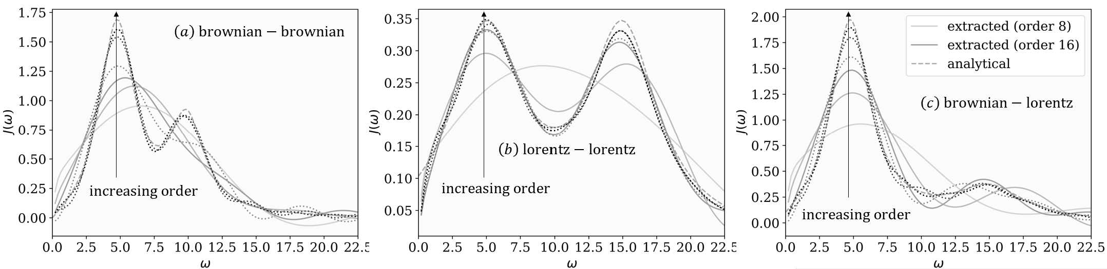
Furthermore, we show how we can inversely obtain for highly structured environments in Fig. 11: in panel (a) , for panel (b) , and for panel (c) . Specifically these are spectral densities that are the additions of brownian-brownian, lorentz-lorentz, and brownian-lorentz spectral densities with different peak frequencies, respectively. It is significant that even for highly structured spectral densities such as these the extraction procedure succeeds, although one would need to go to high orders in the Dyck diagrams.
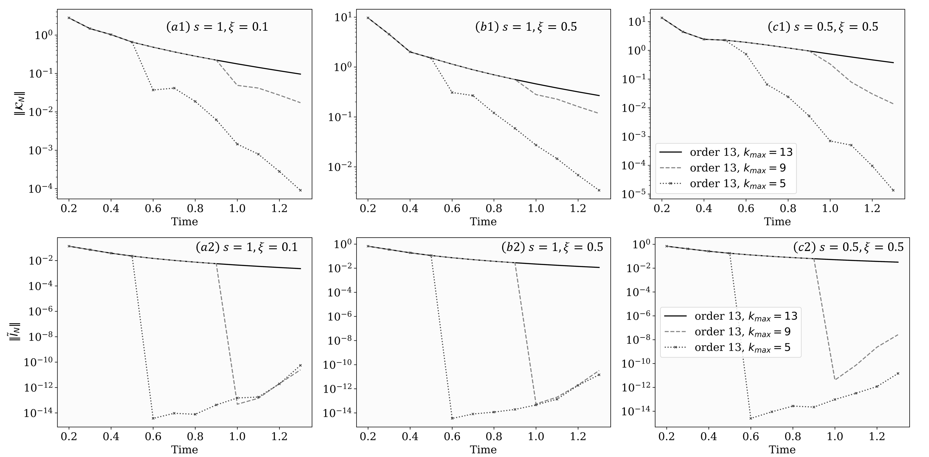
Lastly, we look at how the truncation in affects and vice versa. We construct approximate with truncated (i.e., akin to i-QUAPI). Similarly, we extract effective with truncated (i.e., akin to GQME). We present these results in Fig. (12). Here, we study the three different regimes considered in the main text. In panels (a1), (b1), and (c1), we show the decay of of Dyck order , if we truncate (set for ) at , , and respectively. Here, one observes the error of premature truncation compounds, at e.g., the error of when truncating at is significantly larger than when truncating at . On the other hand, it appears that the effective extracted from this truncated is a poor approximate of the actual (although this makes sense since we impose a hard truncation, for ). This is shown in panels (a2), (b2), and (c2); of Dyck order , at , , and , respectively.
Figure 10: The coefficients inversely calculated (solid line), which perfectly matches the a priori results (crosses). Parameters are identical to Fig.3 in the main text.Figure 11:
Panels (a), (b), and (c): Bath spectral densities extracted through the Dyck diagrammatic method with increasing truncation orders (from white to black colors, and in sequence) compared to exact spectral densities (dashed), see Appendix C. Note that for orders and (dotted), we directly proceed from since the procedure for these high orders are currently infeasible. In all cases, our approach obtains the structured spectral density. For panel (a) the exact spectral density , for panel (b) , and for panel (c) .
Parameters used are: (other parameters are expressed relative to ), , , , , , , and .
Figure 12: Panels (a1), (b1), and (c1): The operator norm of the approximate when we truncate (set for ) at , , and , respectively. The solid line is the exact . Panels (a2), (b2), and (c2): The operator norm of obtained from approximate shown in panels (a1), (b1), and (c1). The solid line indicates the exact .
Parameters used are: (other parameters are expressed relative to ), , , , , and and (panel (a)),
and (panel (b)), or and (panel (c))