SISMIK for brain MRI: Deep-learning-based motion estimation and model-based motion correction in k-space

Abstract

MRI, a widespread non-invasive medical imaging modality, is highly sensitive to patient motion. Despite many attempts over the years, motion correction remains a difficult problem and there is no general method applicable to all situations. We propose a retrospective method for motion quantification and correction to tackle the problem of in-plane rigid-body motion, apt for classical 2D Spin-Echo scans of the brain, which are regularly used in clinical practice. Due to the sequential acquisition of k-space, motion artifacts are well localized. The method leverages the power of deep neural networks to estimate motion parameters in k-space and uses a model-based approach to restore degraded images to avoid ”hallucinations”. Notable advantages are its ability to estimate motion occurring in high spatial frequencies without the need of a motion-free reference. The proposed method operates on the whole k-space dynamic range and is moderately affected by the lower SNR of higher harmonics. As a proof of concept, we provide models trained using supervised learning on 600k motion simulations based on motion-free scans of 43 different subjects. Generalization performance was tested with simulations as well as in-vivo. Qualitative and quantitative evaluations are presented for motion parameter estimations and image reconstruction. Experimental results show that our approach is able to obtain good generalization performance on simulated data and in-vivo acquisitions.

Deep learning, in-vivo, motion correction, motion quantification, MRI.

1 Introduction

MRI is an essential imaging modality in medicine, which suffers unfortunately from a great sensitivity to movements that can deteriorate image quality. Motion occurs sequentially in time and is reflected into the sequential k-space acquisition in a mostly predictable manner (see subsection 2.1). We make the hypothesis that motion parameters can be retrieved from k-space, given knowledge of the acquisition scheme. The latter can be very diverse in MRI, which makes the problem very complex[1].

Deep learning (DL) - a branch of machine learning (ML) that uses deep artificial neural networks (DNNs) - is attractive due to its ability to deliver fast solutions for highly complex problems, which might not be practically solvable by conventional methods. Many solutions, operating in image space and using deep convolutional neural networks for ”image-to-image” motion correction, have been proposed[2, 3, 4, 5, 6, 7]. Although they can produce high quality results, they suffer from reconstruction instabilities[8] such as introducing hallucinations (spurious structures that might be misleading), which is a very significant concern in the medical domain[9, 10, 11]. Thus, it seems preferable to work in k-space rather than image space, due to the locality of motion (MRI acquisition is an inherently sequential process) and also to reduce the dependence to specific contrasts or image structures present in the training datasets.

Other approaches tackle the problem by detecting motion in image space and use a model-based approach for motion parameter estimation and reconstruction, thereby avoiding the risk of hallucinations[12]. Polak et al. used additional low-resolution scout scans as a motion-free reference to guide the search for motion parameters[13]. Applying deep learning directly in k-space seems inherently more difficult, due to its high dynamic range, as opposed to image space. It is also not clear how to properly normalize k-space to make it suitable for deep learning. Regarding approaches operating in k-space rather than image space, recent work by Eichhorn et al. proposed a DL-based approach to classify motion-corrupted k-space lines with performance assessment performed only on simulated datasets[14]. A preliminary investigation to estimate motion from adjacent k-space phase lines, incorporating a model-based correction method was proposed in [15]. The feasibility of this approach was mostly assessed using synthetic rectangle images for which an analytical expression of the Fourier transform is known. Research by Mendes et al. [16] have shown that a modified correlation operation applied on adjacent phase lines allows to estimate translational motion in turbo Spin-Echo acquisitions, (provided that a sufficient turbo factor is used). Hossbach et al. [17] used a deep neural network to quantify rigid-body motion in k-space. However, they used a motion-free reference to estimate motion parameters and only considered the central (64x64) region of k-space.

Other methods, not based on ML/DL, known as ”Autofocusing” - in analogy to optical systems where a sharp image is obtained by adjusting the position of a lens. They use a mathematical formalism (usually formulated as a matrix inversion problem) together with the optimization of an image quality metric (typically similar to Shannon entropy) to estimate motion parameters allowing a reduction of motion artifacts[18, 19, 20, 21].

We propose a novel deep learning-based approach that overcomes the need for a motion-free reference and is able to learn in a wide range of spatial frequency regions of k-space. To avoid the risk of hallucinations, we propose a model-based reconstruction approach that is able to correct motion artifacts when provided with the in-plane rigid-body motion parameters estimated by the proposed DNN. A novel k-space quality metric is also proposed. The idea stems from a 1995 publication, where Wood et al.[22] leveraged visible discontinuities in k-space to detect the occurrences of motion. Using the ESPIRiT multi-coil reconstruction approach[23], and a classical signal processing pipeline, we are able to locate corrupted phase encoding lines and provide a quality score. Moreover, the metric is reference-less. To the best of our knowledge, no k-space quality metric has yet been proposed. Conventional reference-less quality metrics operate in image space [24, 25, 26, 27, 28]. A diagram describing the proposed motion-correction pipeline is provided in Figure 1. It is not intended to cover all possible trajectories in k-space, rather we focus on 2D Spin-Echo sequences with Cartesian sampling to demonstrate the ability of DNNs to retrieve motion parameters in k-space.

The following sections are organized as follows: Section II describes the physical model and the methodology. This entails the design of the k-space quality metric, motion quantification with the proposed DNN, a detailed description of its architecture along with the training procedure. Then, the proposed model-based motion correction method is presented and the section is concluded by a description of the experiments performed. The experimental results are presented in Section III and discussed in Section IV.

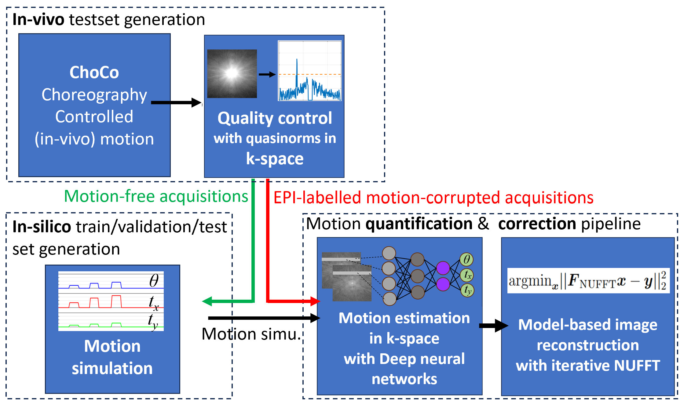
Figure 1: Visualization of the motion acquisition, simulation, quantification and correction pipeline. The quality control metric plays an important role in the development/verification process, in particular, to verify in-vivo motion-corrupted acquisition as well as simulation consistency.

2 Methods

2.1 Description of the problem

The physical process that takes place for each phase encoding line of a classical Spin-Echo acquisition - which we used for our experiments - can be described by the following equation:

$$S_{c}(k_{x},k_{y})=\int\int C_{c}(x,y)\rho(x,y)e^{-i2\pi xk_{x}}e^{-i2\pi yk_{y}}\,dx\,dy$$ (1)

Where the integrals run over the whole field of view, $\rho\in\mathbb{R}$ is the ($T_{1}$ or $T_{2}$) weighted spin density, $C_{c}\in\mathbb{C}$ is the $c$-th coil sensitivity profile, $i^{2}=-1$ and $k_{x}\in\mathbb{R}$, $k_{y}\in\mathbb{R}$ are the wavenumbers in the frequency and phase encoding directions, respectively.

During a classical Spin-Echo acquisition, phase encoding allows the acquisition of a single line of k-space at each TR (in the order of seconds). Frequency encoding is much faster (in the order of milliseconds), therefore, only motion in the phase encoding direction is considered.

When a patient moves during the acquisition of a specific phase encoding line ($k_{y}$), the position-dependent resonance frequency of spins induced by magnetic field gradients introduces a displacement of the acquired points in k-space. This phenomenon typically manifests as artifacts in image space, characterized by the appearance of ”ringing” or ”ghosting” effects. This mismapping can be interpreted as sampling the wrong spatial frequencies, while the patient is static (as opposed to the patient moving while sampling the regular Fourier coefficients). This perspective conceptually leads to the usage of the non-uniform fast Fourier transform (NUFFT) for reconstructing motion-corrupted scans (process described in more details in subsection 2.5).

Rigid-body motion can be described by the following homogeneous matrix:

$$\begin{split}&\begin{pmatrix}1&0&\tau_{x}\\ 0&1&\tau_{y}\\ 0&0&1\end{pmatrix}\begin{pmatrix}\textrm{cos}(\theta)&-\textrm{sin}(\theta)&0\\ \textrm{sin}(\theta)&\textrm{cos}(\theta)&0\\ 0&0&1\end{pmatrix}\begin{pmatrix}1&0&-\tau_{x}\\ 0&1&-\tau_{y}\\ 0&0&1\end{pmatrix}\\ &=\begin{pmatrix}\textrm{cos}(\theta)&-\textrm{sin}(\theta)&-\tau_{x}\textrm{cos}(\theta)+\tau_{y}\textrm{sin}(\theta)+\tau_{x}\\ \textrm{sin}(\theta)&\textrm{cos}(\theta)&-\tau_{x}\textrm{sin}(\theta)-\tau_{y}\textrm{cos}(\theta)+\tau_{y}\\ 0&0&1\end{pmatrix}\end{split}$$ (2)

where $\theta$ is the rotation angle, $\tau_{x}$,$\tau_{y}$ correspond to the distances to the rotation centre, and we define

$$t_{x}:=-\tau_{x}\textrm{cos}(\theta)+\tau_{y}\textrm{sin}(\theta)+\tau_{x}$$ (3)

and

$$t_{y}:=-\tau_{x}\textrm{sin}(\theta)-\tau_{y}\textrm{cos}(\theta)+\tau_{y}$$ (4)

the residual translations associated with a rotation around an arbitrary center $(c_{x},c_{y})$, which can be computed from a reference ”zero center” (e.g., the center of the field of view $(c_{x_{0}},c_{y_{0}}):=(M/2+1,N/2+1)$, where $M$ and $N$ represent the k-space/image matrix dimensions, as $c_{x}=c_{x_{0}}-\tau_{x}$ and $c_{y}=c_{y_{0}}-\tau_{y}$.

The rigid-body motion parameters associated with in-plane rotation around an arbitrary center are therefore $\theta$, $t_{x}$ and $t_{y}$. Our hypothesis posits that, in general, motion-corrupted brain scans acquired with the classical Cartesian Spin-Echo technique can be corrected in a satisfying manner by estimating these three latter parameters, neglecting potential out-of-plane motion.

2.2 k-space quality metric

A quality metric, operating in k-space, is proposed. Motion-corrupted phase lines can be detected in k-space and a quality score can be computed. We noticed that when raw multi-coil k-space data is reconstructed with the ESPIRiT algorithm [23], phase encoding lines corresponding to motion onset undergo a loss of signal with respect to the adjacent ones (in the k-space magnitude). This phenomenon can be explained by the convolution theorem because coil sensitivity profiles (estimated by ESPIRiT) are point-wise multiplied in image space during reconstruction, resulting in a convolution with the coil profile’s Fourier transform in k-space. This leads to signal loss near the discontinuities as shown in Figure 2a. The detection method is as follows. Considering each phase encoding line $k_{y}$ as a vector $\bm{x}\in\mathbb{C}^{n}$, we compute a modified version of its $p$-norm:

$$||\bm{x}||_{p}:=-(\sum_{i=1}^{n}|(\textrm{log}|x_{i}|)|^{p})^{\frac{1}{p}}$$ (5)

Mathematically, if $0<p<1$, then Equation 5 defines a quasinorm rather than a norm, since it fails to satisfy the triangle inequality but retains the two other properties common to all norms (non-negativity and homogeneity). Following computation of the quasinorm, a moving average is performed to smooth the resulting curve and finally compute the first-order discrete derivative. The lines with a significant signal loss can then be detected by thresholding the absolute value of the discrete derivative. The values of both $p$ and the threshold were empirically determined. To improve detection and since Spin-Echo acquisitions are always multi-slice, we take the average of the magnitudes of all the slices and perform the aforementioned procedure. Taking the average has the effect of emphasising signal loss since all slices of the same acquisition experienced the same rigid motion. This is clearly visible in Figure 2. A k-space quality score can then be computed as the absolute value of the detected peaks.

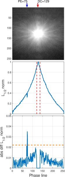
Figure 2: Motion detection with $L_{\frac{1}{2}}$ quasinorms and discrete derivatives. From top to bottom: logarithm of k-space average magnitude, visible loss of signal at phase line 75 where motion occurred (blue arrow) and motion-detection by a single peak above an empirically-determined threshold (corresponding to 0.3 degrees). (In-vivo k-space data from a volunteer who made a 3-degree rotation).

2.3 Simulated and in-vivo datasets

The proposed method leverages deep learning to quantify motion directly in k-space before applying a model-based reconstruction technique to remove motion artifacts. The assumption is that head movements are essentially rigid and in-plane. We considered only the phase encoding direction as the frequency encoding direction is sampled too fast for bulk motion to have any significant effects.

Our approach is based on the hypothesis that motion can be estimated from a limited number of adjacent lines in the phase encoding direction without any motion-free reference.

The proposed deep neural network (DNN) receives a block of consecutive k-space lines in the phase encoding direction as input, organized as a 2-channel tensor of real and imaginary components. The Fourier rotation theorem and the Fourier shift theorem establish corresponding relationships in image space and k-space. A rotation by $\theta$ radians in image space corresponds to a rotation by the same $\theta$ angle in k-space (around the DC point). Translations in image space correspond to phase ramps in k-space. The assumption is that the DNN will be able to learn these relationships and detect and quantify inconsistencies occurring due to a motion event.

Deep learning approaches require large amounts of data, it was hence necessary to simulate motion artefacts to build a training set of adequate size. For this proof of concept, to demonstrate that learning and generalization is possible from k-space without any reference, only one motion event was simulated. Also, multiple DNNs (with the same architecture) were trained on different k-space regions (centered on a given PE line). Therefore, each DNN is in a way ”specialized” for a given line (or more accurately, in a limited neighbourhood of the given line).

Raw, motion-free, classical multi-slice T1w Spin-Echo k-space data for the training set was gathered from a clinical 3T MRI system (MAGNETOM Prisma fit, Siemens Healthineers, Erlangen, Germany) through a stringent manual inspection process. Out of 300 acquisitions, only 43 were deemed acceptable (motion-free) and included in the dataset. With an average of 30 slices per acquisition, this resulted in around 1290 slices in total, which were used as a basis for simulation. The number of coils per acquisition varied between 16 and 58, an in-plane resolution of 1 mm and slice thickness of 4 mm. Although, the matrix size and FOV may vary from scan to scan, all the data were resized to 256 $\times$ 256.

Simulations were performed on each coil individually by applying rotations in image space around a random center, empirically chosen corresponding to real-like motion. For each simulated PE line, the corresponding k-space rows in the motion-free slice were replaced by the corrupted k-space ones.

Around 600k training examples were simulated for each phase encoding (PE) line on which the DNN was trained. A validation set of 10k simulations and a simulated testset of 10k were also generated. The validation and test sets simulations were performed on 6 additional motion-free acquisitions unseen during training.

For demonstrating the network’s capabilities in different k-space regions (spatial frequencies), the following PE lines were selected: 30,50,75,90 and 105. Motion parameters were drawn from a Gaussian distribution with mean $\mu=0$ and $\sigma=1.5$ for $\theta$ (degrees) and the rotation center offsets ($c_{x}$ and $c_{y}$) were uniformly drawn from the range $[-40,40]$ (pixels) which resulted in $t_{x}$ and $t_{y}$ in (approximately) the range $[-2.5,2.5]$ (pixels). Also, two different motion speeds were simulated: ”instantaneous”, i.e., abrupt transition from $0$ to $\theta$ degrees and a ”slower” speed with a small $1\times 3$ convolution kernel around the transition.

Finally, an ”in-vivo” testset was produced following the ChoCo protocol described in [29]. We asked 15 volunteers to perform different video-controlled head choreographies, to produce known motion artifacts on classical T1w Spin-Echo acquisitions, with similar parameters as those used for training. With TR=500 ms, TE=12 ms, TA=2 min. The FOV was roughly 220$\times$220 mm, the voxel size of 1$\times$1$\times$4 mm, a matrix size of 256$\times$256 and 16 coils. After data quality checks (motion-free), only the data from 5 subjects was kept for data augmentation.

We generated ”empirical labels” by motion estimation using rigid-body registration of a preliminary EPI training sequence, according to the proposed ChoCo motion protocol[29]. These labels were used for DNN performance evaluation.

2.4 DNN: Design, Objectives and Training Strategy

The proposed DNN model architecture is similar to that of a LeNet [30] or AlexNet[31] convolutional feedforward artificial neural network. These networks can be conceptually separated into two parts: a feature-extractor followed by a classifier[32]. In our case, the second part is rather performing regressions since it has to output 3 real valued parameters: the rotation angle $\theta$ (degrees) and two translations $t_{x}$ and $t_{y}$ (pixels). The full network architecture is shown in Figure 3. It searches for motion parameters in segments of a full k-space, hence we called it SISMIK: Search In Segmented Motion Input (in) K-space.

2.4.1 Input normalization

For artificial neural networks to learn effectively, the relevant data points should all be in a homogeneous range. In order to cope with the high dynamic range due to the high DC component, we computed mean and standard deviation maps from all motion-free k-spaces in our dataset. During DNN training, each minibatch was then normalized by subtracting the mean and dividing by the standard deviation maps, point-wise. Following this normalization, the dynamic range of the k-spaces becomes suitable for deep learning.

2.4.2 DNN training strategy

Training of the DNN was carried out using supervised learning on simulated datasets. An input consisting of a small k-space window around motion onset was provided along with the ground truth motion vector of 3 real-valued parameters: $(\theta,t_{x},t_{y})$ for this single motion event. Therefore, the input consists of a motion-free region followed by a ”transition” (typically one or two lines, depending on motion speed) and the final rotated region. A window size $w$ of 9 was empirically chosen for our experiments. We used the mean squared error (MSE) loss function as can be justified by the maximum likelihood principle for modelling Normally distributed errors [33].

SISMIK starts by extracting features at different levels through its convolutional layers (see Figure 3 ”feature extractor block”). The first three $1\times 3$ (padded) convolutions do not change the input size and allow a transformation of the input into a more suitable representation for further analysis. This can be thought of as the network performing an encoding of the $w$ phase lines into an internal representation, without merging them. Subsequently, a $w\times 3$ convolution collapses the feature map size into a shape of $256\times 256$. This step allows the network to combine the information of all the lines in the input simultaneously. This is the penultimate part of the feature extractor block (see Figure 3) and allows the network to obtain high level features, before performing one more convolution step and a final regression of the motion parameters (performed by two dense layers). We may think of the first $1\times 3$ convolutions as performing some kind of pre-processing of the input before a compression into a single channel which is subsequently downsampled by max-pooling and flattened to be fed to the final fully connected (dense) block. The latter performs the final regression of the 3 output rigid-body motion parameters. Training was performed with the PyTorch deep learning library using an Adam optimizer with an adaptive learning rate starting at $10^{-6}$, a batch size of 128, Tikhonov regularization at $10^{-6}$, a single 0.25 dropout layer and early stopping (based on the validation set performance). It is important to note that the initial learning rate of $10^{-6}$ had to be empirically chosen significantly lower than is usual for Adam (i.e., usually closer to $10^{-3}$), otherwise learning diverges. We used a total of 100 epochs for training with random shuffling of the trainingset each time. This was justified by the fact that no more improvements could be observed and the learning rate dropped below $10^{-8}$.

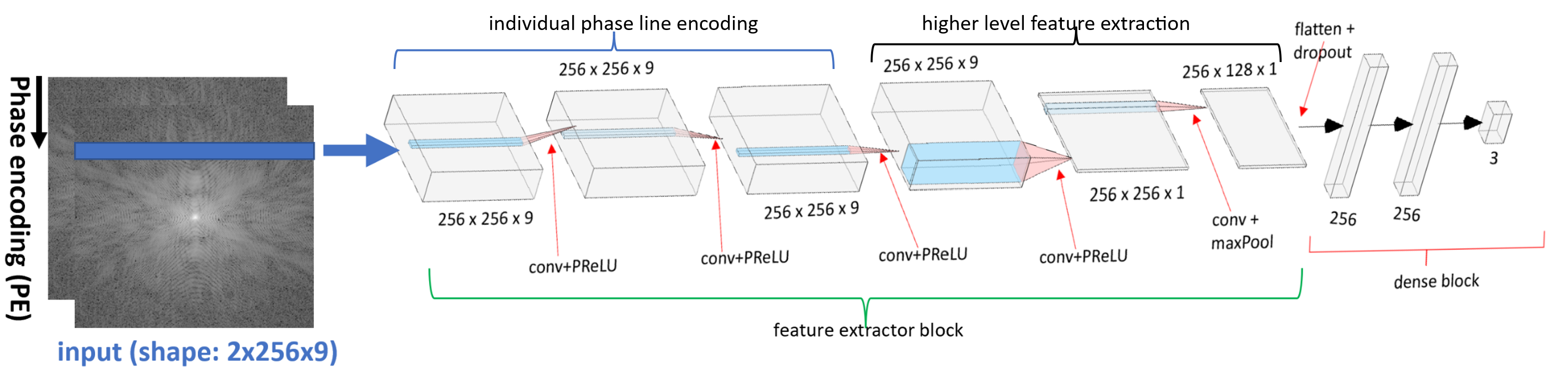
(a)

Figure 3: DNN architecture: 5 convolutional layers forming the ”feature extractor” block, followed by max-pooling and a dense block for the final estimation of the 3 in-plane rigid-body motion parameters. Notice that the first 3 convolutional layers scan trough the feature maps, leaving its shape unchanged until the penultimate convolution collapses it into a single channel.

2.5 Model-based motion correction

A non-uniform Fourier matrix can be built from the knowledge of the rotational motion trajectory that occurred during acquisition. An (inverse) non-uniform Fourier transform (NUFFT) can then be applied on the corrupted k-space data to recover a motion-free complex image. We used Fessler’s NUFFT toolbox for a very fast and memory-efficient implementation of this procedure in Matlab[34, 35]. An example trajectory for a single motion event can be seen in Figure 4.

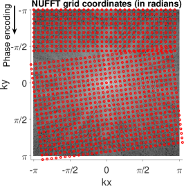
Figure 4: Example of NUFFT trajectory for a single motion event occurring in the upper half of k-space. The grid is undersampled for better visualization.

Translational motion can be corrected by applying point-wise opposite phase ramps to the corrupted k-space lines. The motion correction process can be mathematically described by the following steps. Let $\Phi\in\mathbb{C}^{N\times N}$ the dephasing matrix be:

$$\large\Phi=e^{-i2\pi\bm{k}_{x}\odot\bm{t}_{x}}e^{-i2\pi\bm{k}^{\top}_{y}\odot\bm{t}^{\top}_{y}}$$ (6)

where $\odot$ is the Hadamard product, $\bm{k}_{x}$, $\bm{k}_{y}$ are vectors of spatial frequency coordinates and $\bm{t}_{x}$, $\bm{t}_{y}$ are vectors of estimated translations (for all spatial frequency coordinates, including the motion-free ones, for which the parameters are equal to zero).

$$\large\widetilde{\bm{Y}}=\bm{Y}\odot\Phi$$ (7)

where $\bm{Y}\in\mathbb{C}^{N\times N}$ is the measured motion-corrupted k-space matrix and $\widetilde{\bm{Y}}\in\mathbb{C}^{N\times N}$ the phase-corrected k-space.

$$\large\widehat{\bm{x}}=\bm{F}^{\dagger}_{\textrm{NUFFT}}\textrm{vec}(\widetilde{\bm{Y}})$$ (8)

where $\widehat{\bm{x}}\in\mathbb{C}^{N^{2}}$ is the reconstructed (vectorized) image, the dagger ($\dagger$) denotes the Hermitian adjoint of $\bm{F}_{\textrm{NUFFT}}$, the non-uniform Fourier transform operator and $\textrm{vec}(\widetilde{\bm{Y}})\in\mathbb{C}^{N^{2}}$ is the notation for a vectorized matrix, i.e., $\widetilde{\bm{Y}}\in\mathbb{C}^{N\times N}$ has all its columns flattened into a long vector of $N^{2}$ components.

In practice, better results, with no significant computational cost, are obtained by iteratively computing:

$$\large\widehat{\bm{x}}_{\textrm{LSQR}}=\textrm{argmin}_{\bm{x}}||\bm{F}_{\textrm{NUFFT}}\bm{x}-\textrm{vec}(\widetilde{\bm{Y}})||^{2}_{2}$$ (9)

for about 10 or 12 iterations (it takes less than a second), which we will refer to as the iterative least-squares NUFFT.

Image reconstruction using inverse NUFFT was performed on the ESPIRiT multi-coil combined k-space.

2.6 Experiments and performance evaluation

Dataset simulations were performed on a HPC cluster and neural network training was done on a mid-range server equipped with a CUDA-compatible GPU with 12GB of VRAM.

2.6.1 k-space quality metric optimization

To find an optimal threshold (see Figure 2) we performed specific motion simulations described thereafter. Since the degradation of k-space is related to the magnitude (and number) of motion events, it is necessary to obtain a good motion detection performance. The latter was assessed from simulations calibrated to cover the range of PE lines and a discretization of angle magnitudes to cover the range on which the DNN was trained. The PE lines were chosen between 10 and 250 by steps of 5 with 12 lines removed around the DC line. The chosen angles were $\theta\in\{0,0.01,0.1,0.2,0.3,0.4,0.5,1.0,1.5,...,3.5,4.0\}$. We considered $\theta<0.3$ as ”no motion”. This choice was dictated by the fact that motion artifacts are barely visible at $\theta\simeq 0.5$ degrees and, in general, not visible at all to the human eye below that. With two different speeds (same as for training) and 10 different motion-free acquisitions used for simulating the artifacts, this resulted in a total of 5244 (full multi-slice volume) simulations.

ROC curves were plotted to give an estimation of the trade-off between the true positive rate and the false positive rate for different values of $p$ according to Equation 5. This allowed to empirically determine the best $p$ norm value.

2.6.2 Motion estimation accuracy

Motion parameter estimation accuracy was evaluated on in-silico test sets (with motion simulations performed on motion-free acquisitions that were unseen during training) using the RMSE and Pearson correlation coefficients between the ground truth and the network’s predictions. For in-vivo test sets, the median DNN prediction for all slices of each acquisition was used as the estimated label for the corresponding acquisition (since all slices in the same acquisition undergo the same rigid motion). The RMSE was reported for each case.

2.6.3 Motion correction quality

Next in our approach, a comparison of the reconstruction quality with respect to an autofocusing approach is proposed. The freely available GradMC method was chosen [21] because it uses a model-based correction approach, similar to ours, based on a matrix inversion formalism using an entropy metric[18, 36] to assess image quality. PSNR and SSIM metrics were computed from motion-free ground truth and motion-corrected simulations for both strategies.

In-vivo motion correction quality was assessed using information gain as a quantitative metric. Information gain can be defined as the difference between the Shannon entropy of a corrupted image and the corresponding restored image. An improvement in image quality should decrease the entropy, resulting in positive information gain. We also provide representative examples of in-vivo corrected images for qualitative reconstruction assessment.

GradMC was run for 100 iterations for each testset case. This number of iterations was chosen because no significant drop in entropy occurred afterwards.

3 Experimental results

3.0.1 k-space quality metric

Motion detection results are presented as ROC (Receiver Operator Characteristic) curves to assess the achievable performance in terms of true positive rate and false positive rate. It also allows us to demonstrate how an empirical detection threshold and an $L_{p}$-quasinorm value can be selected.

Results are presented in 5a for 5244 motion simulations on a range of PE lines covering the whole k-space expect for a small region near the center (DC) as described in subsubsection 2.6.1. ROC curves for 7 different $p$-quasinorm values were computed for 1000 different thresholds and are presented in (5a). A true positive rate close to $90$% can be obtained for a false positive rate near $4$% by choosing $L_{p}$ with $\frac{1}{16}\leq p\leq\frac{1}{2}$. Higher order norms ($p\geq 1$) have a strictly worse performance.

5ab shows how the optimal threshold of 0.02 found for $L_{1/2}$ allows a discrimination between 3 different k-space quality classes.

3.0.2 Motion quantification with SISMIK

Motion parameter estimations obtained with SISMIK are presented for increasing wavenumbers and the RMSE and Pearson correlation metrics were used to provide two complementary views of the DNN’s performance. RMSE and Pearson correlation results are shown in Figure 6. Performance increases with decreasing spatial frequency, as expected following the SNR distribution in k-space acquisitions. Translations ($t_{x}$, $t_{y}$) exhibit lower correlation than the rotation angles and seem more difficult to learn, the correlation metric being independent of error magnitude. For an intermediate spatial frequency (PE=75) the DNN achieves an RMSE around 0.55 degrees for the rotation angle and an RMSE around 0.35 pixels for the translations. Rotation angle estimation results obtained on simulated testsets ($\sim$ 10k samples) can be seen in Figure 7. A rolling window of 100 data points was used to display the mean and standard deviation. SISMIK starts to exhibit a larger standard deviation at the extremities of the range on which it was trained but otherwise shows good performance.

For in-vivo testsets acquired with the ChoCo protocol[29], performance is as follows. Experiments were performed with volunteers on PE75. The RMSE of DNN estimations compared to ChoCo labels was 0.59 degrees for the rotation angle and 1.21 pixels for $t_{y}$ and 0.18 pixels for $t_{x}$. The in-vivo angle RMSE is very close to the in-silico RMSE (0.55). The $t_{y}$ RMSE is higher due to the presence of two significant outliers, which correspond to the large negative information gains for subject 4 in Figure 10.

3.0.3 Motion correction from DNN predictions

The last stage of the pipeline entails reversing the effects of motion using a model-based approach by building a NUFFT matrix from the estimated rotation angles following phase ramp cancellation with the formula in Equation 7. Qualitative results for simulations are shown in 8a and are also compared to the GradMC method. Quantitative results presented as boxplots for a range of angles and PE lines covering different motion intensities and k-space regions are shown in 8b and 8c. NUFFT reconstructions with SISMIK estimations result in a median PSNR of 37.8 dB and a median SSIM of 0.98. For the same slices corrected with GradMC, a median PSNR of 29.7 dB and SSIM of 0.93 are obtained.

By only focusing on the ”Corrupted” and ”SISMIK” boxplots in Figure 8 (b) and (c), we can compare the PSNR and SSIM metrics of corrupted and restored slices, solely from SISMIK estimations, with respect to the motion-free ground truth used for simulation. All the restored slices obtain a PSNR $>$ 30 dB, whereas all the corrupted ones are below 30 dB. For the SSIM metric, all corrupted slices are below 0.91 and all the restored ones (except for a few outliers) are above 0.97. Overall, this demonstrates that the proposed DNN estimations allow a model-based restoration with NUFFT that can completely separate the motion-corrupted PSNR and SSIM distributions from the restored ones.

Two representative examples of in-vivo motion-corrupted ChoCo slices and their restored versions based on DNN predictions are presented in Figure 9. These qualitative results show that DNN estimations were accurate enough to allow the removal of most of the motion artifacts.

Quantitative results for 5 in-vivo ChoCo subjects are shown in Figure 10. The latter distributions show that DNN estimations tend to get worse with increasing angle magnitude. It also shows that all (except 3 outliers) of the smaller angles (around 2 degrees) were well estimated. It can also be observed that 80% of the subjects (4/5) exhibit positive information gain for more than 75% of all their restored acquisitions. All the acquisitions (small, medium and large angles) of subject 2 were restored with positive information gain. Subject 4 represents a failure of the DNN to estimate the larger angles accurately.

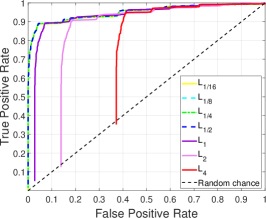
(a)

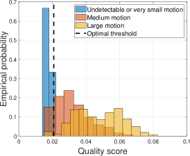
(b)

Figure 5: (a) ROC curves for 7 different $L_{p}$ values and 1000 different thresholds. For $p<1$, curves align closely, indicating that they provide similar sensitivity and specificity. A value of 0.3° was defined as the ”empirical zero”, below which any motion is deemed undetectable. (b) Histograms divided into 3 classes with the optimal threshold found for $p=0.5$ indicate that the data is separable.

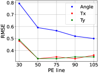
(a)

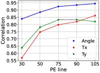
(b)

Figure 6: DNN training performance (RMSE and Pearson correlation) for the estimation of in-plane rigid-body motion parameters. The x-axis goes from the highest (PE=30) spatial frequency to the lowest (PE=105) used in our experiments. Performance increases as we move towards lower spatial frequencies. (DC at PE=129).

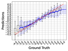
(a) PE = 30

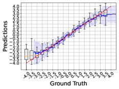
(b) PE = 75

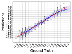
(c) PE = 105

Figure 7: DNN estimations of the rotation angle for 3 different k-space regions: high (PE=30), medium (PE=75) and lower (PE=105) spatial frequencies. The latter obtains the best performance. The rolling mean and standard deviation (rolling window of 100 points) are shown in dark blue and as the shaded regions around it, respectively.

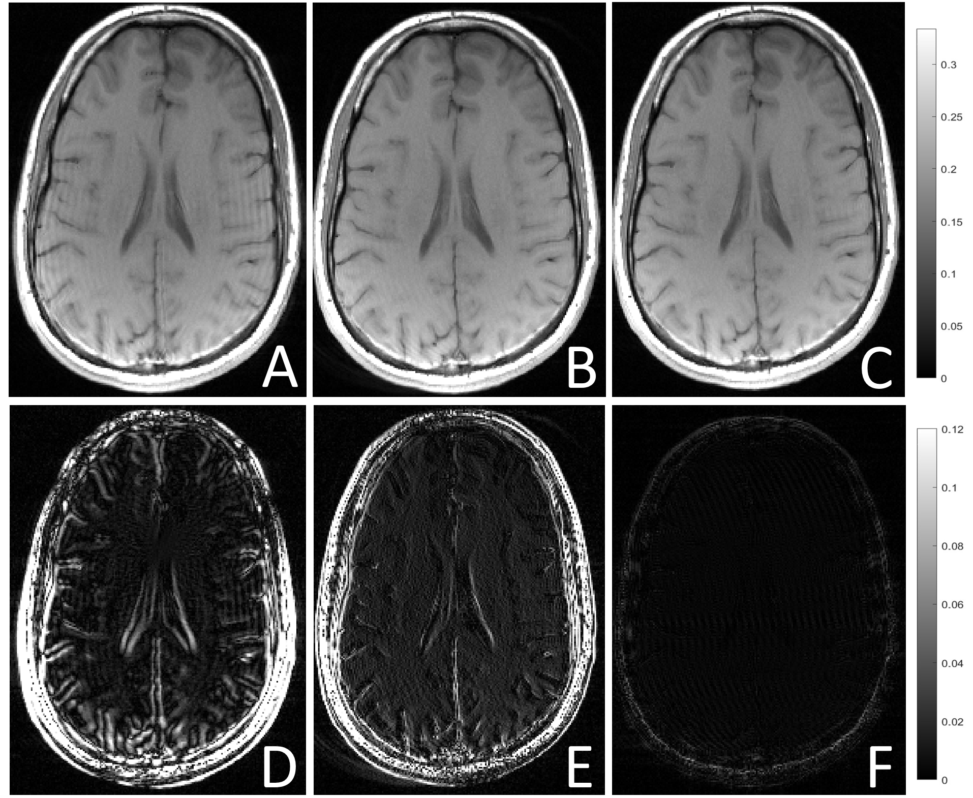
(a)

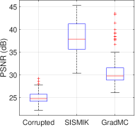
(b)

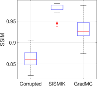
(c)

Figure 8: (A) Representative example of simulated corruption (approx. 3 degrees rotation). (B) Restored with GradMC. (C) Restored with NUFFT from DNN predictions. (D,E,F) are the absolute difference to the reference motion-free acquisition used for simulation. PSNR and SSIM distributions for simulations over a range of [-4°, 4°] for different subjects and slices as shown In boxplots (b) and (c). In (b) the performance of SISMIK is compared to the GradMC method. In (c) we can observe that the distributions of PSNRs and SSIMs of the corrupted and restored (both with SISMIK) slices, do not overlap.

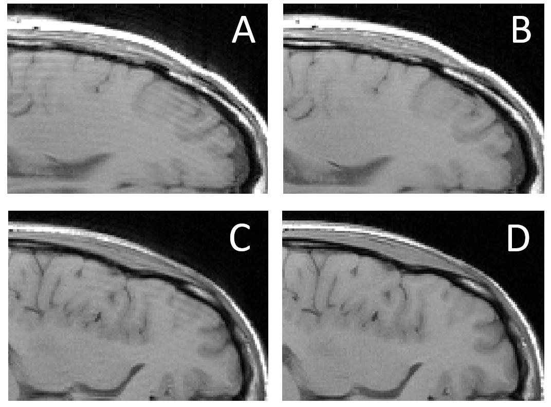
Figure 9: (A and C) Representative examples of classical T1w Spin-Echo acquisitions corrupted in-vivo following the ChoCo procedure for generating controlled motion artifacts. (B and D) Restored images by phase cancellation and iterative NUFFT reconstruction from DNN motion parameter estimations. (The two rows show the same anatomical region for two different subjects.)

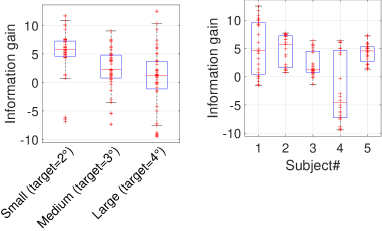
Figure 10: (Left) information gain distribution for 3 (in-vivo ChoCo) angle categories corresponding (roughly) to 2, 3 and 4 degrees. Performance decreases with increasing angle magnitude. (Right) Information gain distributions for 5 ChoCo in-vivo subjects. All have more than 75% positive information gain, except subject 4.

4 Discussion

The experimental results demonstrate that it is possible to learn rigid-body motion parameters in k-space without a motion-free reference even in the higher spatial frequencies.

In order to evaluate the performance of SISMIK in high spatial frequencies, the system was trained on 5 different PE lines. The assumption being that as we deviate further from DC, the noise level increases, thereby complicating the learning process. This assumption is verified, but generalization performance in higher spatial frequencies - which were excluded in previous work [17] - is still sufficient to allow for qualitatively and quantitatively acceptable motion correction quality, as shown in Figure 6. Restoring high spatial frequencies is especially important to preserve fine details provided by state-of-the art MRI technology.

Larger rotation angles are more difficult to learn in part because we have limited the standard deviation of the simulation distribution for the proof of concept and may also be related to increasing loss of information in the edges of k-space (a.k.a. ”pie slice” phenomenon[37, 38]). This information loss also results in residual artifacts even when reconstructing a slice from known simulation parameters.

A k-space quality metric is also proposed. It leverages the fact that multi-coil ESPIRiT reconstruction enhances motion transitions in k-space, which are detectable using quasinorms and discrete derivatives, followed by thresholding. For Spin-Echo acquisitions, it is possible to leverage the Hermitian symmetry of k-space to detect signal drops near the corresponding motion affected PE lines[39, 40]. This approach works to some extent but Hermitian symmetry is not good enough in practice to yield better results than the proposed method. This quality metric serves as a valuable tool during the dataset generation process. It offers a convenient method for performing ”sanity checks” to ensure that simulated or in-vivo motion events are correctly localized in k-space. For phase encoding lines that are not too close to DC, the ”k-space quality score” can provide information about motion magnitude as shown in 5ab. The proposed k-space quality metric could also be a good complement or alternative to image-based metrics.

Working in k-space confers the advantage of precise motion localization, in contrast to image space where it is distributed everywhere. The proposed DNN is able to leverage local information with a narrow window of only 9 PE lines to estimate motion parameters. This comes at the cost of having multiple DNNs specialized for each phase encoding line using the same architecture, just trained on a different k-space block. In practice we have observed that the networks are able to obtain a similar performance for PE lines in a close neighbourhood (around $\pm 5$ lines). Therefore, a potential five-fold reduction in the number of trained models may be possible, but this requires further investigation and testing. However, once training is complete, all the phase encoding lines of a motion-corrupted k-space slice may be passed in parallel, hence incurring no cost related to the ”multi-network” requirement.

It is a well-known fact that deep neural networks are prone to ”hallucinations”, e.g., the creation of spurious structures in a brain image, which can lead to diagnostic errors [11, 41]. Therefore, we used a model-based reconstruction approach rather than an ”image to image” strategy such as [6] or [4], embedding a full reconstruction framework inside a DNN. In the worse case, the model-based approach will fail to remove enough artefacts but it will not introduce false structures or remove existing ones. When the motion-estimating-DNN is able to provide the correct parameters and the in-plane rigid-body assumption holds, then artifacts may be significantly removed.

A comparison with the GradMC model-based method[21] was performed. The latter uses an ”autofocusing” approach based on the optimization of an entropy metric to estimate motion parameters of a corrupted MRI acquisition. Figure 8 shows that the proposed DNN’s estimations of the motion parameters followed by phase cancellation and iterative NUFFT achieves a higher increase in PSNR and SSIM. GradMC is also less robust in the sense that it can often diverge and is unable to find the optimal motion parameters. For this comparison, GradMC was initialized with motion parameters obtained from the DNN, in order to avoid a divergent behaviour. This highlights the fact that such autofocusing approaches can benefit from better initialization. The proposed DNN can provide these estimations and therefore reduce the computational burden of such iterative methods, which may require in the order of minutes to correct a single slice.

Overall, SISMIK is able to restore motion-corrupted slices simulated from a parameter space that corresponds to realistic patient motion. In practice, with properly padded head-coils, only small rotation angles are expected[42, 43].

Figure 8 also shows that the PSNR and SSIM distributions of motion corrupted and restored images are consistent and do not overlap after motion estimation and reconstruction with the proposed approach, showing improvement in all simulations.

Figure 9 shows representative examples of corrupted slices along with the restored versions, which qualitatively highlights the ability of SISMIK to correctly estimate in-vivo motion parameters. Small angles are better estimated than larger ones, resulting in better image quality (higher information gain) for angles $\leq 2$ degrees per motion event, in general (Figure 10 (left) ). Information gain distributions for all in-vivo subjects - acquired with the ChoCo protocol - and all angles (2,3 and 4 degrees for each subject) are presented in Figure 10 (right). All subjects show more than 75% information gain, except subject 4. This indicates that the DNN has successfully estimated motion parameters in-vivo for the vast majority of cases, with failures predominantly isolated to a single subject. It may be related to the fact that this subject has performed larger angles than the others during the ChoCo in-vivo acquisitions.

Different directions are possible for improving the approach. It is possible to train the same DNN architecture with simulations performed on individual coils rather than multiple coils combined with ESPIRiT, as was performed for this proof of concept. The signal drops in k-space due to convolution with the coil sensitivity profile’s Fourier transform will no longer occur. We will need to investigate whether this change enhances or hampers the learning process. Another possibility involves adapting the method to 3D acquisitions. This extension should be achievable as long as the k-space data is presented to the network in the order of its sequential acquisition. This requirement exists because the DNN employs local temporal motion information to estimate the motion trajectory. In particular, this could allow restoring motion corrupted 3D MP-RAGE acquisitions, which are widely used in the clinical setting.

5 Conclusion

In this study, a novel deep learning-based approach for quantifying in-plane rigid-body motion in k-space was proposed. It is novel in at least two aspects: it is reference-less and is able to learn in the higher k-space spatial frequencies, despite an increasing amount of noise. A novel k-space quality metric was also proposed, which leverages signal drops arising from convolutions in k-space when ESPIRiT reconstruction is performed. The experimental results demonstrate that the proposed DNN is able to obtain good generalization performance for motion estimation followed by correction of corrupted images obtained in-silico as well as in-vivo.

References

- [1] Maxim Zaitsev, Julian Maclaren and Michael Herbst “Motion artifacts in MRI: A complex problem with many partial solutions” In Journal of Magnetic Resonance Imaging 42.4 Wiley Online Library, 2015, pp. 887–901
- [2] Thomas Küstner et al. “Retrospective correction of motion-affected MR images using deep learning frameworks” In Magnetic resonance in medicine 82.4 Wiley Online Library, 2019, pp. 1527–1540
- [3] K Sommer et al. “Correction of motion artifacts using a multiscale fully convolutional neural network” In American Journal of Neuroradiology 41.3 Am Soc Neuroradiology, 2020, pp. 416–423
- [4] Junchi Liu, Mehmet Kocak, Mark Supanich and Jie Deng “Motion artifacts reduction in brain MRI by means of a deep residual network with densely connected multi-resolution blocks (DRN-DCMB)” In Magnetic resonance imaging 71 Elsevier, 2020, pp. 69–79
- [5] Soumick Chatterjee et al. “Retrospective motion correction of MR images using prior-assisted deep learning” In arXiv preprint arXiv:2011.14134, 2020
- [6] Kamlesh Pawar, Zhaolin Chen, N Jon Shah and Gary F Egan “Suppressing motion artefacts in MRI using an Inception-ResNet network with motion simulation augmentation” In NMR in Biomedicine 35.4 Wiley Online Library, 2022, pp. e4225
- [7] Ben A Duffy et al. “Retrospective correction of motion artifact affected structural MRI images using deep learning of simulated motion” In Medical Imaging with Deep Learning, 2022
- [8] Vegard Antun et al. “On instabilities of deep learning in image reconstruction and the potential costs of AI” In Proceedings of the National Academy of Sciences 117.48 National Acad Sciences, 2020, pp. 30088–30095
- [9] Joseph Paul Cohen, Margaux Luck and Sina Honari “Distribution matching losses can hallucinate features in medical image translation” In Medical Image Computing and Computer Assisted Intervention–MICCAI 2018: 21st International Conference, Granada, Spain, September 16-20, 2018, Proceedings, Part I, 2018, pp. 529–536 Springer
- [10] Nina M Gottschling, Vegard Antun, Ben Adcock and Anders C Hansen “The troublesome kernel: why deep learning for inverse problems is typically unstable” In arXiv preprint arXiv:2001.01258, 2020
- [11] Sayantan Bhadra, Varun A Kelkar, Frank J Brooks and Mark A Anastasio “On hallucinations in tomographic image reconstruction” In IEEE transactions on medical imaging 40.11 IEEE, 2021, pp. 3249–3260
- [12] Melissa W Haskell et al. “Network Accelerated Motion Estimation and Reduction (NAMER): Convolutional neural network guided retrospective motion correction using a separable motion model” In Magnetic resonance in medicine 82.4 Wiley Online Library, 2019, pp. 1452–1461
- [13] Daniel Polak et al. “Scout accelerated motion estimation and reduction (SAMER)” In Magnetic Resonance in Medicine 87.1 Wiley Online Library, 2022, pp. 163–178
- [14] Hannah Eichhorn et al. “Deep Learning-Based Detection of Motion-Affected k-Space Lines for T2*-Weighted MRI” In arXiv preprint arXiv:2303.10987, 2023
- [15] Rajesh Rajwade “Magnetic Resonance Imaging motion correction in k-space: Detecting, estimating and correcting the bulk motion artifacts in k-space data”, 2019
- [16] Jason Mendes, Eugene Kholmovski and Dennis L Parker “Rigid-body motion correction with self-navigation MRI” In Magnetic Resonance in Medicine: An Official Journal of the International Society for Magnetic Resonance in Medicine 61.3 Wiley Online Library, 2009, pp. 739–747
- [17] Julian Hossbach et al. “Deep learning-based motion quantification from k-space for fast model-based MRI motion correction” In Medical Physics Wiley Online Library, 2022
- [18] David Atkinson et al. “Automatic correction of motion artifacts in magnetic resonance images using an entropy focus criterion” In IEEE Transactions on Medical imaging 16.6 IEEE, 1997, pp. 903–910
- [19] Armando Manduca et al. “Autocorrection in MR imaging: adaptive motion correction without navigator echoes” In Radiology 215.3 Radiological Society of North America, 2000, pp. 904–909
- [20] Wei Lin and Hee Kwon Song “Improved optimization strategies for autofocusing motion compensation in MRI via the analysis of image metric maps” In Magnetic resonance imaging 24.6 Elsevier, 2006, pp. 751–760
- [21] Alexander Loktyushin, Hannes Nickisch, Rolf Pohmann and Bernhard Schölkopf “Blind retrospective motion correction of MR images” In Magnetic resonance in medicine 70.6 Wiley Online Library, 2013, pp. 1608–1618
- [22] Michael L Wood, Mansur J Shivji and Peter L Stanchev “Planar-motion correction with use of k-space data acquired in Fourier MR imaging” In Journal of Magnetic Resonance Imaging 5.1 Wiley Online Library, 1995, pp. 57–64
- [23] Martin Uecker et al. “ESPIRiT—an eigenvalue approach to autocalibrating parallel MRI: where SENSE meets GRAPPA” In Magnetic resonance in medicine 71.3 Wiley Online Library, 2014, pp. 990–1001
- [24] Jeffrey P Woodard and Monica P Carley-Spencer “No-reference image quality metrics for structural MRI” In Neuroinformatics 4 Springer, 2006, pp. 243–262
- [25] Bénédicte Mortamet et al. “Automatic quality assessment in structural brain magnetic resonance imaging” In Magnetic Resonance in Medicine: An Official Journal of the International Society for Magnetic Resonance in Medicine 62.2 Wiley Online Library, 2009, pp. 365–372
- [26] Ilkay Oksuz “Brain MRI artefact detection and correction using convolutional neural networks” In Computer Methods and Programs in Biomedicine 199 Elsevier, 2021, pp. 105909
- [27] Michael E Osadebey et al. “Standardized quality metric system for structural brain magnetic resonance images in multi-center neuroimaging study” In BMC medical imaging 18 Springer, 2018, pp. 1–19
- [28] Thomas Küstner et al. “A machine-learning framework for automatic reference-free quality assessment in MRI” In Magnetic resonance imaging 53 Elsevier, 2018, pp. 134–147
- [29] Oscar Dabrowski et al. “Choreography Controlled (ChoCo) brain MRI artifact generation for labeled motion-corrupted datasets” In Physica Medica 102 Elsevier, 2022, pp. 79–87
- [30] Yann LeCun and Yoshua Bengio “Convolutional networks for images, speech, and time series” In The handbook of brain theory and neural networks 3361.10 Citeseer, 1995, pp. 1995
- [31] Alex Krizhevsky, Ilya Sutskever and Geoffrey E Hinton “Imagenet classification with deep convolutional neural networks” In Advances in neural information processing systems 25, 2012
- [32] Yann LeCun, Léon Bottou, Yoshua Bengio and Patrick Haffner “Gradient-based learning applied to document recognition” In Proceedings of the IEEE 86.11 Ieee, 1998, pp. 2278–2324
- [33] Ian Goodfellow, Yoshua Bengio and Aaron Courville “Deep Learning” http://www.deeplearningbook.org MIT Press, 2016
- [34] Jeffrey A Fessler and Bradley P Sutton “Nonuniform fast Fourier transforms using min-max interpolation” In IEEE transactions on signal processing 51.2 IEEE, 2003, pp. 560–574
- [35] Jeffrey A Fessler “Michigan image reconstruction toolbox” Ann Arbor (MI): Jeffrey Fessler, http://web.eecs.umich.edu/~fessler/irt/fessler.tgz, 2018
- [36] PG Batchelor et al. “Matrix description of general motion correction applied to multishot images” In Magnetic Resonance in Medicine: An Official Journal of the International Society for Magnetic Resonance in Medicine 54.5 Wiley Online Library, 2005, pp. 1273–1280
- [37] David Atkinson and Derek LG Hill “Reconstruction after rotational motion” In Magnetic Resonance in Medicine: An Official Journal of the International Society for Magnetic Resonance in Medicine 49.1 Wiley Online Library, 2003, pp. 183–187
- [38] Frank Godenschweger et al. “Motion correction in MRI of the brain” In Physics in medicine & biology 61.5 IOP Publishing, 2016, pp. R32
- [39] E Mark Haacke, ED Lindskogj and Weili Lin “A fast, iterative, partial-Fourier technique capable of local phase recovery” In Journal of Magnetic Resonance (1969) 92.1 Elsevier, 1991, pp. 126–145
- [40] David Moratal, A Vallés-Luch, Luis Martí-Bonmatí and Marijn E Brummer “k-Space tutorial: an MRI educational tool for a better understanding of k-space” In Biomedical imaging and intervention journal 4.1 Department of Biomedical Imaging, University of Malaya, 2008
- [41] Keri Stephens “Investigating Hallucinations in Medical Imaging” In AXIS Imaging News Anthem Media Group, 2022
- [42] Arne Wagner et al. “Quantification and clinical relevance of head motion during computed tomography” In Investigative radiology 38.11 LWW, 2003, pp. 733–741
- [43] Zidan Yu et al. “Exploring the sensitivity of magnetic resonance fingerprinting to motion” In Magnetic resonance imaging 54 Elsevier, 2018, pp. 241–248