Improving Semantic Correspondence with Viewpoint-Guided Spherical Maps

Abstract

Recent progress in self-supervised representation learning has resulted in models that are capable of extracting image features that are not only effective at encoding image-level, but also pixel-level, semantics. These features have been shown to be effective for dense visual semantic correspondence estimation, even outperforming fully-supervised methods. Nevertheless, current self-supervised approaches still fail in the presence of challenging image characteristics such as symmetries and repeated parts. To address these limitations, we propose a new approach for semantic correspondence estimation that supplements discriminative self-supervised features with 3D understanding via a weak geometric spherical prior. Compared to more involved 3D pipelines, our model only requires weak viewpoint information, and the simplicity of our spherical representation enables us to inject informative geometric priors into the model during training. We propose a new evaluation metric that better accounts for repeated part and symmetry-induced mistakes. We present results on the challenging SPair-71k dataset, where we show that our approach demonstrates is capable of distinguishing between symmetric views and repeated parts across many object categories, and also demonstrate that we can generalize to unseen classes on the AwA dataset.

1 Introduction

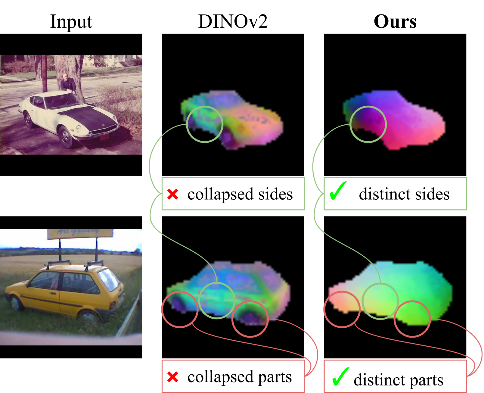
Figure 1: Image features from self-supervised methods such as DINOv2 [39] have been shown to be effective at discovering parts and regions of objects. However, these features have two main limitations: (i) they fail to correctly distinguish object symmetries, e.g. the left and right side of the car have the same features and (ii) they struggle to distinguish individual parts, e.g. the wheels are represented by the same features irrespective of their location on the car. Our approach, which makes use of a weak geometric spherical prior, addresses these issues. Note, for DINOv2 we visualize the thee dimensional PCA projection of the features and for our approach we visualize our learned spherical mapping.

Semantic correspondence (SC) estimation aims to find local regions that correspond to the same semantic entities across a collection of images, where each image contains a different instance of the same object category [30]. SC has been studied from both the supervised [9, 58, 26] and unsupervised [50, 2] perspectives. Thanks to the recent progress in self-supervised learning (SSL) [6, 59, 39], recent SSL-based approaches have been shown to obtain strong performance on multiple benchmarks [1, 54, 2]. However, they often do so by acting as simple part detectors, without having any 3D understanding of object extent, or relative location of object parts. As these models are typically trained using only 2D image augmentation-based objectives, they are not able to learn 3D-aware representations, and often converge to similar features for object parts that share appearance but not fine-grained semantics.

The two main failure modes of current methods are depicted in Fig. 1. First, they are often confused by the symmetries that objects can exhibit (e.g. left versus right side of a car), producing reflected versions of the feature maps when presented with the two different sides of a symmetric object. Second, they predict similar features for similar looking parts (e.g. the front left versus back left wheel of a car), making it hard to discriminate between part instances. Such symmetries and repeated structures are ubiquitous in both human-made and naturally occurring object categories.

We posit that these shortcomings can be addressed by introducing explicit 3D knowledge into correspondence learning, by giving the model the possibility to choose between multiple repeated parts, or teaching it to understand that some object parts might not be visible in all images. Indeed, scene-based correspondence pipelines use geometric verification in order to guarantee robustness in their matches [43], while other works have shown that detailed 3D meshes can be used to discover category-based correspondences through a render-and-compare pipeline [61, 29]. However, these approaches typically require 3D mesh supervision which is difficult and costly to obtain at scale.

Motivated by the limitations and promise of the recent SSL representations [39], we propose a novel method that incorporates the missing 3D geometry into object representations. In particular, we make use of a weak 3D prior by representing object features on the surface of a sphere which encodes both geometry and appearance information. Our method consistently maps features corresponding to the same semantic parts (e.g. left headlight of a car) in images of different object instances to the same spherical coordinates, hence enabling a 3D aware and accurate correspondences. However, learning such a mapping without the ground-truth 3D supervision is nontrivial, because of repeated parts and object symmetries. To this end, we propose to use much weaker supervision via coarse viewpoint annotations to help our model separate these confusing features. We couple this with geometric constraints to prevent collapsed representations for repeated parts. As a result, our method learns to separate object parts based on their position and spatial configuration in an image.

Furthermore, we point out that the standard evaluation metric for SC, Percentage of Correct Keypoints (PCK) is not able to properly evaluate symmetry-related failures. As it only considers keypoints that are visible in both the source and target image, it does not penalize methods that match, for example, a left wheel with a right one. Rather than simple accuracy-based metric, we argue that average precision is a more robust scoring mechanism and propose a new metric, Keypoint Average Precision (KAP), to account for potential spurious matches.

Our contributions are thus: i) a novel SC approach that learns to separate visually similar parts by mapping them to different location on a sphere, ii) a set of simple geometric constraints that force separation of visually similar parts during training, and iii) a new evaluation protocol that better accounts for the failure cases of current methods.

2 Related work

Image matching. Visual correspondences were first explored as exact matches between different views of the same scene with applications to stereo vision [37, 24], object detection [33, 14], structure from motion [52, 20, 43], and SLAM [19, 12]. Correspondences can also be computed across pixels in the frames of a video, which is referred to as optical flow [5, 7]. Traditionally they are found by computing hand-crafted visual descriptors such as SIFT [32], HOG [11], or ORB [42], which are matched across images.

Semantic correspondence (SC). In SC estimation, the goal is not only to find matches across different views of the exact same object instance, but instead across different instances of the same object category. This more challenging case was originally explored in SIFT Flow [30]. While earlier work [30] match two images through densely sampled SIFT [32] features, later works extended pairwise correspondence learning to a global matching problem [60] and established region correspondences using object proposals and their geometric relations over dense descriptors [17]. Subsequently it was demonstrated that CNNs trained with only image-level supervision could be used to discover correspondences [31], paving the way for many deep learning correspondence systems [10, 18, 58, 26]. Typical correspondence-specific CNN architectures rely on aggregating features along the depth of a network [53, 35, 58] or use 4D convolutions spanning two images simultaneously [40]. More recently, transformers have been shown to be particularly suited to correspondence discovery thanks to their attention mechanism [9].

In parallel, early attempts were made towards unsupervised correspondence discovery [50, 27, 2], and recent developments in transformer-based self-supervised methods [6, 39, 59] are closely bridging the gap with fully supervised methods. Without using explicit correspondence supervision, these model are able to discover salient and robust features, which subsequent works have applied to detect semantic correspondences to great success, often surpassing supervised methods [1, 54, 57, 46]. Recently, it has also been shown that the features from generative image models can be used for SC [22, 57, 48]. Closely related to our method, some approaches propose to create category-wide representations by aligning self-supervised feature maps [38, 16]. Unlike our method, these works are purely 2D, and find correspondences between images without knowing the underlying 3D structure of the world which renders them incapable of distinguishing different sides of objects (e.g. left vs. right side of a car).

3D priors for correspondence. Understanding the 3D geometry of an object is a valuable signal when trying to estimate correspondence across different instances of the category. Inspired by this, multiple approaches have proposed using 3D priors in order to aid correspondence estimation. Annotated 3D models have been used to make predictors aware of self-occlusions [61]. Subsequently, canonical surface mappings using 3d models coupled with a dense parameterization to discover image correspondences were developed [29, 45, 8]. Our approach uses a similar parameterization, but does not require 3D models. An alternative approach involves the estimation of 3D models of object categories from image supervision alone [23, 15, 25, 36, 55, 3], from which correspondences are extracted. However, this is very challenging by itself, requiring complex pipelines capable of modeling accurate mesh deformations, pose, and rendering, which are all failure-prone.

In contrast, we use a sphere as a weak 3D prior, where our goal is to map pixel locations in images to the surface of the sphere, such that the same part of an object maps to the same location on the sphere and is consistent across different instances of the object. When the precise camera viewpoint is known, sparse correspondences can be automatically discovered through constrained geometric optimization [47] or through a neural field [56]. The requirement for accurate poses is however strict, and these models cannot easily be trained from coarse pose supervision.

3 Method

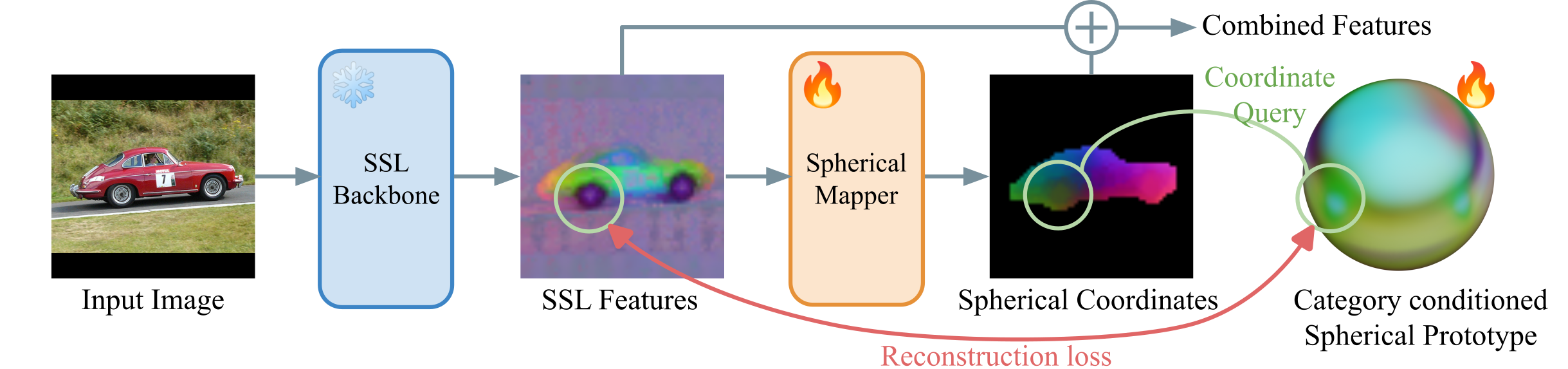
Figure 2: Overview of our semantic correspondence estimation approach. We begin by extracting features from a frozen self-supervised backbone. These features are then mapped to the surface of a sphere via a learned module, and the resulting spherical coordinates are used to query a jointly learned prototype, providing the supervision signal (Sec. 3.2). The sphere is used to enforce weak geometric priors for each category (Sec. 3.3). During inference, SSL features are combined with spherical coordinates (Sec. 3.4).

3.1 Problem statement

Given an unordered monocular image collection, we wish to learn a mapping $f:(\bm{I},x)\rightarrow\bm{z}$ that takes in an RGB image $\bm{I}:\Lambda\rightarrow\mathbb{R}^{3}$, $\Lambda\subset\mathbb{R}^{2}$ and a pixel $x\in\Lambda$ to an $n$-dimensional embedding $z\in\mathcal{Z}\subset\mathbb{R}^{n}$. In particular, we would like $f$ to map semantic concepts from different instances of the same category (e.g. center of front-right wheel of a car) to the same point in the embedding space $\mathcal{Z}$. Formally, $f(\bm{I},x)=f(\bm{I}^{\prime},x^{\prime})$, when the pixels $x$ in $\bm{I}$, and $x^{\prime}$ in $\bm{I}^{\prime}$ correspond to the same semantic part and instance. In practice, the corresponding location for $(\bm{I},x)$ in $\bm{I}^{\prime}$ can be obtained by finding the nearest neighbor of $f(\bm{I},x)$ in the embedding space, i.e. $\operatorname*{arg\,min}_{x^{\prime}}d_{\mathcal{Z}}(f(\bm{I},x),f(\bm{I}^{\prime},x^{\prime}))$, where $d_{\mathcal{Z}}$ is a distance function over $\mathcal{Z}$. For simplicity, we will use $f(\bm{I})$ to refer to the feature map obtained by evaluating $f$ on all pixels of $\bm{I}$.

An ideal embedding function should be general enough as to not only match related semantic parts across different object instances (e.g. match the front-left wheel across two different models of car), but also specific enough to distinguish between different part instances within the same object instance (e.g. front-left wheel vs. front-right wheel). Learning this from image-based self-supervision alone is a challenging task due to similar appearance of repeated parts and self-occlusion. As a result, it is quite challenging for correspondence estimators to learn that cars have four distinct wheels from single images alone without explicit supervision.

Therefore, it is beneficial to endow a correspondence estimator with priors about the underlying 3D structure of objects. Previous methods have done this using detailed 3D meshes [61, 29], via a render-and-compare approach. This is limited by the availability of such meshes, and the lack of precise viewpoint estimation for rendering. Instead, following [50, 51], we propose to use a simplified 3D structure, specifically a sphere $S^{2}\subset\mathbb{R}^{3}$ (denoted as $S$ for simplicity). To do this, we make the simplifying assumption that the object categories of interest are roughly homeomorphic to spheres (i.e. objects without holes). While this may at first appear particularly ill-adapted for some categories, e.g. bicycles, the geometric simplicity of $S$ provides a well-behaved parameterization of an object’s surface while allowing easy computation of geometric constraints that can be used to separate visual and semantic similarity. In particular, $S$ provides a simple geodesic distance through the dot product, making it straightforward to push different semantic parts apart. We use this property to separate repeated object features.

Formally, we are interested in building a spherical mapping $f_{S}(\bm{I},x)$ that maps pixels in $I$ to the surface of $S$. Unlike an arbitrary $n$ dimensional space, $S$ forms an object-centric specific coordinate system, where each region represents a distinct semantic part and instance on the surface of the object. However, in the absence of ground truth correspondences, ensuring the semantic consistency of our spherical mapping function is very challenging. [50] enforces correspondence between image pairs through synthetically augmenting training images via thinplate splines. Unfortunately such synthetic augmentations does not produce realistic 3D transformations such as 3D rotations which can result in the self-occlusion of parts. To enforce such consistency, similar to [38, 16], we formulate the learning objective as one of aligning pretrained SSL features between different instances of an object category. While those approaches use flat atlases $\mathbb{R}^{2}\rightarrow\mathcal{Z}$, we build a spherical prototype $S_{\mathcal{Z}}:S^{2}\subset\mathbb{R}^{3}\rightarrow\mathcal{Z}$ that maps a point on the surface of the sphere $s\in S^{2}$ to a feature vector $\mathbf{z}\in\mathcal{Z}$. This formulation has two important benefits. First, the input domain of $S_{\mathcal{Z}}$ is simply $S$, meaning that it does not depend on $I$, and it is shared across all images, constituting a category-based map (Section 3.2). Second, and in contrast to [38, 16], because we chose the output of $f_{S}$ to lie on the surface of a sphere, we can use it to enforce 3D priors during training (Section 3.3).

3.2 Learning correspondences on a sphere

As discussed earlier, self-supervised methods like DINO [6, 39] natively exhibit impressive semantic characterization of local image regions. While DINO features struggle to differentiate between repeated object parts, they often succeed in identifying these parts across object instances can be used to determine if two regions contain similar parts. Starting with such a pretrained self-supervised model $\phi$ as our backbone feature extractor, our training objective aims to solve the alignment between the instance feature maps $\phi(\bm{I}):\Lambda\rightarrow\mathbb{R}^{d}=\mathcal{Z}$ and the spherical prototype.

Intuitively, for a given category, the spherical prototype $S_{\mathcal{Z}}$ should be able to reconstruct any self-supervised feature map $\phi(\bm{I})$ when queried on the coordinates predicted by $f_{S}$, i.e. $S_{\mathcal{Z}}(f_{S}(\bm{I},x))$ must closely approximate $\phi(\bm{I},x)$ for any $\bm{I},x$. Even if $S_{\mathcal{Z}}$ encodes a perfect category prototype, it will be unable to encode information about the image background. We therefore use instance masks $M(\bm{I})$ at training time, restricting loss computation to only the pixels on an object’s surface. In practice, these can be obtained using pretrained segmentation models [21]. Thus, given a training image $\bm{I}$ and a pixel location $x$, our primary training objective to learn the parameters of $f_{S}$ and $S_{\mathcal{Z}}$ can be formulated as the minimization of

$$\mathcal{L}_{rec}=M(\bm{I},x)\times\Gamma\left(\phi(\bm{I},x),S_{\mathcal{Z}}\circ f_{S}(\bm{I},x)\right),$$ (1)

where $\Gamma$ is the cosine distance between the two inputs. Our spherical prototypes are implemented with a neural network that maps points in $\mathbb{R}^{3}$ to $\mathcal{Z}$. Importantly, each input $s\in S^{2}\subset\mathbb{R}^{3}$ must be mapped independently, meaning that it should correspond to a unique point $\mathbf{z}\in\mathcal{Z}$, irrespective of which instance it comes from or where in the image this part is located. In order to account for multiple categories, and to encourage information sharing between closely related ones, we use a single network conditioned on a category embedding. In practice, $S_{\mathcal{Z}}$ is a visual transformer [13] without self-attention, but with cross-attention between image tokens and a single category token $\mathbf{c}$ which is a one hot embedding of the category.

3.3 Enforcing geometric priors

The above spherical reconstruction formulation alone offers little benefit over matching the self-supervised features from $\phi$ directly, especially considering the low dimensionality of the intermediate spherical space, which is not guaranteed to be well-behaved. However, this spherical constraint enables the computation of simple geometric priors that can be enforced during training.

Viewpoint regularization.

Many object categories exhibit some form of symmetry which can make it particularly challenging for image-based models to distinguish between the sides of a car as their predictions also tend to be symmetric, creating spurious correlations between distinct parts (see Fig. 1). One potential way of addressing this challenge without using dense groundtruth correspondence is to exploit viewpoint information of the object instance.

An interesting property of using a spherical prototype to represent an object category is that it can easily be used to infer an object’s viewpoint with respect to the camera. We posit that the average coordinate of a spherical map of an image $\bm{I}$, $f_{S}(\bm{I})$ can be viewed as a coarse approximation of the camera viewpoint under which the object is seen, e.g. right side views should be approximately mapped to the right side of the sphere, and left side views to the left. Intuitively, thinking of $f_{S}$ as a mapping from image pixels to the object’s surface, the visible parts of an object should roughly be those closest to the camera, while the others should be hidden by self-occlusion.

By using groundtruth camera viewpoint $v_{I}$, we enforce the average direction of the spherical map $\mu(f_{S}(\bm{I}))$ to align with $v_{I}$. When this is satisfied, symmetric views must be mapped to different parts of the sphere. While precise viewpoint information is hard to obtain, but we observe it is sufficient to use coarse relative viewpoint supervision between images. In practice, $v_{I}$ is discretized among a small number of bins, and we simply enforce that the correlation between viewpoints from two images equals that of their average spherical maps,

$$\mathcal{L}_{vp}=\sum_{I,I^{\prime}}||v_{I}\cdot v_{I^{\prime}}-\mu(f_{S}(\bm{I}))\cdot\mu(f_{S}(\bm{I}^{\prime}))||^{2}.$$ (2)

Relative distance loss.

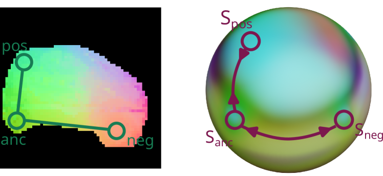
Figure 3: Illustration of our relative distance loss $\mathcal{L}_{rd}$. The left image shows a spherical map from which a triplet of points is sampled. The right image is the category-conditioned prototype, with the corresponding 3D positions of the sampled points. As the positive patch is closer to the anchor on the image compared with the negative, its corresponding $s_{pos}$ position on the sphere is pulled towards the anchor $s_{anc}$, and reciprocally.

As noted earlier, current self-supervised extracted features can confuse repeated object repeated parts. Depending on the target goal, this can be desirable, if the parts do indeed belong to the same part category. However, this is detrimental for dense correspondence estimation as the parts may actually be different part instances, e.g. left versus right leg. It can be hard to distinguish between these based on their appearance alone and additional geometric context is required.

One trivial way of encoding this context is by making the assumption that similar parts that appear in different locations on an image (i.e. not beside each other) are in fact different instances of the same semantic part. Therefore, we would like to enforce the property on our predicted spherical maps that distant pixels in the image should be mapped far part on the sphere. Due to scale variation, distance on the image plane is hard to link to distances on the surface of the sphere. However, we can reformulate this property as a relative distance comparison using a triplet. Given three points $a$, $b$ and $c$ on an image $\bm{I}$, and their corresponding positions $s_{a}=f_{S}(\bm{I},a),s_{b}$ and $s_{c}$ on the sphere, the ordering between distances should be preserved, that is:

$$||a-b||\leq||a-c||\iff\Gamma(s_{a},s_{b})\leq\Gamma(s_{a},s_{c}).$$ (3)

In reality, this does not hold for distances along an object’s surface, which the sphere is supposed to represent, partly due to perspective. For example, in the case of a long train seen from a near frontal view, parts at the back of the train might appear very close to the front in the image, even though they are very far in 3D space. Nevertheless, we find that this is still an effective prior for discouraging repeated part instances from being mapped to the same location.

During training, point triplets $(a,b,c)$ are randomly sampled among pixels that belong to the object. Among each such triplet, we chose an anchor location $anc=a$, a positive location $pos=\operatorname*{arg\,min}_{x\in\{b,c\}}||a-x||$, and a negative location $neg=\operatorname*{arg\,max}_{x\in\{b,c\}}||a-x||$ (see Fig. 3). We can then define a triplet margin loss as:

$$\begin{split}\mathcal{L}_{rd}=\max(&\Gamma(f_{S}(\bm{I},anc),f_{S}(\bm{I},pos))\\ -&\Gamma(f_{S}(\bm{I},anc),f_{S}(\bm{I},neg))+\delta,0),\end{split}$$ (4)

where $\delta$ is a hyperparameter which specifies the margin. A useful side product of this formulation is that it encourages the spherical maps to be smooth, as strong discontinuities would produce a large anchor to positive distance.

Orientation loss.

A final advantage of using $S^{2}$ as a latent space is that it is an orientable 2D space, just like images. Therefore, enforcing that $f_{S}$ preserves orientation prevents spurious matches between symmetric views. Intuitively, if a point $a$ appears on the right side of $b$ in the image, then $s_{a}$ must appear in the same side of $s_{b}$. Given a point triplet as defined earlier, this can be enforced by making sure that the determinant $d_{I}=\text{det}(b-a,c-a)$ positively correlates with $d_{S}=\text{det}(P_{a}(s_{b})-s_{a},P_{a}(s_{c})-s_{a})$, where $P_{a}$ is the linear projection to the plane tangent to $S^{2}$ at $s_{a}$.

As objects can have complex geometries, it is impossible to determine exactly what the determinant of a sphere triplet should be. However, we can assume that image triplets of large determinants should also have large determinant on the sphere, as a change of sign in determinant indicates the relative orientation on the sphere has been inverted. In practice, we randomly sample image triplets $(a,b,c)$ and select those whose image determinant $d_{I}$ is higher than a threshold $d_{\tau}=0.7$, while swapping $b$ and $c$ if $d_{I}$ is negative. Then, we enforce the determinant of the corresponding sphere triplet to be at least $d_{\tau}$,

$$\begin{split}\mathcal{L}_{o}=\begin{cases}0&\mbox{if }d_{I}<d_{\tau}\\ max(d_{\tau}-d_{S},0)&\mbox{if }d_{I}\geq d_{\tau}.\end{cases}\end{split}$$ (5)

		plane	bicycle	crow	ship	wine-bottle	bus	car	cat	chair		dog	horse	motorcycle	walking			train	tv	avg
Custom	CATS [9]	52.0	34.7	72.2	34.3	49.9	57.5	43.6	66.5	24.4	63.2	56.5	52.0	42.6	41.7	43.0	33.6	72.6	58.0	49.9
	MMNet+FCN [58]	55.9	37.0	65.0	35.4	50.0	63.9	45.7	62.8	28.7	65.0	54.7	51.6	38.5	34.6	41.7	36.3	00.077.7	62.5	50.4
	SCorrSan [26]	57.1	40.3	78.3	38.1	51.8	57.8	47.1	67.9	25.2	71.3	63.9	49.3	45.3	49.8	48.8	40.3	00.077.7	69.7	54.4
DINOv1	DINOv1 [6]	44.3	26.8	57.6	22.0	29.3	32.8	19.7	54.0	14.9	40.1	39.3	29.3	29.0	37.0	20.0	28.2	40.6	21.1	32.6
	ASIC [16]	57.9	25.2	68.1	24.7	35.4	28.4	30.9	54.8	21.6	45.0	47.2	39.9	26.2	48.8	14.5	24.5	49.0	24.6	37.0
	Ours	47.1	26.0	70.9	21.8	37.5	34.9	32.4	60.0	23.2	53.6	48.5	42.5	28.3	42.7	21.1	41.9	39.7	41.7	39.7
SD	DIFT [48]	63.5	54.5	80.8	34.5	46.2	52.7	48.3	77.7	39.0	76.0	54.9	61.3	53.3	46.0	00.057.8	57.1	71.1	00.063.4	57.7
	SD [57]	63.1	55.6	80.2	33.8	44.9	49.3	47.8	74.4	38.4	70.8	53.7	61.1	54.4	55.0	54.8	53.5	65.0	53.3	56.1
DINOv2	DINOv2 [39]	72.7	62.0	85.2	41.3	40.4	52.3	51.5	71.1	36.2	67.1	64.6	67.6	61.0	00.068.2	30.7	62.0	54.3	24.2	56.2
	DINOv2 + SD [57]	73.0	00.064.1	00.086.4	40.7	52.9	55.0	53.8	78.6	45.5	77.3	64.7	69.7	63.3	69.2	58.4	67.6	66.2	53.5	63.3
	Ours (sphere only)	46.7	28.8	66.3	33.0	36.5	66.6	59.1	74.9	25.4	65.7	50.1	52.7	27.1	13.7	15.8	46.6	73.5	36.7	45.5
	Ours	76.9	61.2	85.9	00.042.1	48.4	00.073.3	00.067.2	00.080.0	00.046.3	00.080.2	00.066.7	00.071.2	00.066.0	63.9	36.2	00.068.6	67.8	42.2	00.063.6
	Ours + SD	00.074.8	64.5	87.1	45.6	00.052.7	77.8	71.4	82.4	47.7	82.0	67.3	73.9	67.6	60.0	49.9	69.8	78.5	59.1	67.3

Table 1: Keypoint matching scores on SPair-71k evaluated using PCK@0.1 with macro-averaging for the summary scores. We present our approach using DINOv1 [6] features (middle rows) and DINOv2 [39] features (bottom rows). In both cases, we improve over the DINO only baselines and are superior to fully supervised methods (top rows). Bold entries are best per category and underlined are second-best.

3.4 Correspondence via combined representations

During inference, it is possible to directly query the spherical maps $f_{S}$ of two images to obtain correspondences using the cosine distance. That is, for an image pair $\bm{I},\bm{I}^{\prime}$ and a query location $q$ on $\bm{I}$, its location in $\bm{I}^{\prime}$ can be computed as

$$p^{*}=\operatorname*{arg\,min}_{p}\Gamma(f_{S}(\bm{I},q),f_{S}(\bm{I}^{\prime},p)).$$ (6)

While this protocol is sound, it comes with two important drawbacks. First, $f_{S}$ produces spherical maps for the whole image, including the background, meaning segmentation masks would be required at inference time to prevent the emergence of spurious matches. Second, the spherical map is designed to be a smooth parameterization of the object surface, making it susceptible to missing fine detail. A slightly incorrect mapping $f_{S}(\bm{I},q)+\epsilon$ has a high probability of finding a match in a nearby region of the correct match $f_{S}(\bm{I}^{\prime},p^{*})$ if both maps are smooth. In comparison, SSL feature maps can exhibit strict feature separation, e.g. wheel features are very different from other nearby non-wheel features, making it unlikely that a wheel pixel ends up finding a nearest neighbor among nearby non-wheel pixels.

To mitigate this issue, we make use of the feature maps that are already computed by the self-supervised backbone network $\phi$, in a similar way to supervised correspondence approaches that aggregate features from a network [53, 35, 58]. Existing literature has shown that DINO features are particularly effective at differentiating between the foreground and background [1], removing the need for inference-time segmentation. To leverage these DINO features, we reformulate Eq. 6 as the combination of self-supervised features and spherical locations:

$$\begin{split}p^{*}={\operatorname*{arg\,min}}_{p}&\;\alpha\;\Gamma(f_{S}(\bm{I},q),f_{S}(\bm{I}^{\prime},p))\\ +&(1-\alpha)\;\Gamma(\phi(\bm{I},q),\phi(\bm{I}^{\prime},p)),\end{split}$$ (7)

where $\alpha$ is a hyperparameter that balances each term.

Image
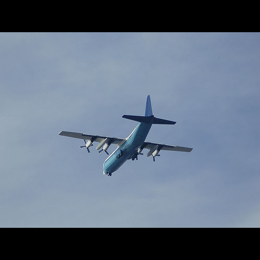
DINOv2
SD
DINOv2+SD
Sphere

Figure 4: Qualitative comparison of dense correspondence maps. For DINOv2, SD, and DINO+SD features we perform PCA on the segmented object features independently for each category, then visualize the three main components. Note that the SD and DINO+SD features are not completely equivalent to the ones used to compute matches, but are provided here for illustration. Spherical maps from $f_{S}$ (Sphere) for our approach are visualized directly. Our spherical maps correctly identify the different sides of objects, whereas other features fail to capture these differences.

4 Experiments

Implementation details. We build our models on DINOv1-B/8 [6] and DINOv2-B/14 [39] backbones. Training masks are obtained using a pretrained Mask R-CNN model [21]. Our spherical mapper consists of a linear dimension reduction layer halving the number of features, a visual transformer block with self-attention, and a final linear layer with an output dimension of three. The resulting feature map is then normalized pixel-wise so that its output values lies on the surface of $S^{2}$. The dimensionality reduction layer, while not strictly necessary, is helpful considering the small number of images used during training, while the transformer block helps in disentangling sides and repeated parts by allowing global reasoning between image patches.

The final loss term is computed as $\mathcal{L}=\mathcal{L}_{rec}+\lambda_{rd}\mathcal{L}_{rd}+\lambda_{o}\mathcal{L}_{o}+\lambda_{vp}\mathcal{L}_{vp}$. We set $\lambda_{rd}=\lambda_{o}=0.3$ and $\lambda_{vp}=0.1$, and $\delta=0.5$ to encourage feature separation. To perform matching in Eq. 7, $\alpha$ is set to $0.2$ so that we leverage the highly discriminative DINO features, while using the sphere as a symmetry and repetition-breaking mechanism. Our model is trained for a total of 200 epochs using the Adam optimizer [28].

Datasets. Following existing work [26, 16, 57], we evaluate our method primarily on the Spair-71k dataset [34], which contains images from 18 different object categories. The evaluation set contains between 600 and 900 image pairs, each of which are annotated with the keypoints that are visible in both images. We train our model on the Spair-71k training split on all categories simultaneously, without using any keypoint annotations. Additionally, we evaluate on the AwA-pose dataset [4], which contains images from 35 quadruped categories, annotated with keypoints. We also present results by training on the Freiburg cars dataset [44]. This dataset was collected by densely sampling approximately 100 images each around 48 different car instances. The higher image count, coupled with 360^o dense sampling, enables us to learn a more detailed spherical prototype.

4.1 SPair-71k results

We first evaluate on the task of keypoint transfer between pairs of images using Spair-71k [34]. We present quantitative per-category results in Tab. 1, along with macro-averaged scores as the number of per-category pairs varies greatly. We split the models according to their backbone: custom supervised models, DINOv1-based, SD-based, and DINOv2-based. A striking preliminary observation is the effectiveness of DINOv2, surpassing supervised approaches on most categories. While its success can partially be attributed to evaluation biases [2], this demonstrates the effectiveness of large scale learned self-supervised features.

Using a DINOv1 backbone, our model improves over its backbone on most categories, and over ASIC [16] on average. When combined with the DINOv2 backbone, our model provides improvements on all but two categories. A clear pattern can be identified, with strongest improvements being observed over blob-like symmetric objects with repeated parts (+21.0 on bus and +15.7 on car), while spherical mapping hinders performance on highly deformable categories (-4.3 on person), or high-genus objects for which a sphere is a poor surface prior (-0.8 on bicycle). Our model performs slightly better compared to DINO+SD [57], while requiring a fraction of the computational cost at inference time. Finally, following [57] we evaluate adding Stable Diffusion (SD) [41] features to our method at inference time, which yields further improvements. This illustrates that spherical maps and SD features capture different facets of the correspondence problem.

The qualitative visualization shown in Fig. 4 illustrates these improved results. Our model correctly maps the two opposite sides of the cars to different sphere regions, while other feature maps look extremely similar, even when looking at two opposite sides of an object, with the notable exception of SD on birds. The fact that such similarities exist between opposite views suggest that the utility of baselines such as DINOv2 would be quite limited in real scenarios.

	plane	bicycle	crow	ship	wine-bottle	bus	car	cat	chair		dog	horse	motorcycle	walking			train	tv	avg
DINOv2 [39]	53.5	54.0	60.2	35.5	44.4	36.3	31.7	61.3	37.4	54.7	52.5	51.5	48.8	48.2	37.8	44.1	47.4	38.2	46.5
SD [57]	44.4	48.5	54.5	31.5	45.2	32.7	30.0	68.4	35.8	55.2	47.9	48.1	44.8	42.3	00.044.5	39.2	52.7	00.051.2	45.4
DINOv2 + SD [57]	52.0	55.9	59.2	34.7	49.0	36.0	32.5	70.3	39.8	59.8	53.1	52.4	50.6	50.4	47.8	46.2	53.3	49.8	49.6
Ours (sphere only)	38.4	34.2	53.9	33.0	37.9	49.7	43.4	00.071.7	29.8	57.1	45.8	42.5	32.4	27.0	29.5	37.1	00.057.4	36.0	42.1
Ours	60.7	51.2	63.1	00.038.4	45.0	55.9	00.045.7	69.7	00.040.4	00.063.2	00.054.8	00.054.3	00.051.2	00.048.7	38.8	00.047.9	55.5	42.2	00.051.5
Ours + SD	00.058.9	00.054.2	00.062.2	39.6	00.046.6	00.054.5	47.1	76.2	40.9	65.3	57.3	56.1	54.2	47.4	43.7	49.4	62.4	52.0	53.8

Table 2: Keypoint matching scores on SPair-71k evaluated using KAP@0.1 with macro-averaging for the summary scores.

Average precision evaluation. While issues with symmetries are clear in Fig. 4, we argue that the PCK metric fails to account for them as it is only computed between keypoints that appear both in the source and target image. Hence, models that predict high similarity between two visually similar but semantically different keypoints will not be penalized. PCK can partly account for repetition-related mistakes if the parts appear simultaneously in both images, but it does not penalize symmetry-related issues, like mistaking the left and right side of a car, as the corresponding keypoints do not appear simultaneously. PCK was initially proposed for simpler cases where keypoints were assumed to be always be visible -e.g. faces, different instances in the same pose, but as benchmark become more challenging, a more robust protocol should be used. To illustrate how much these failure cases impact SSL models, we propose an alternative evaluation metric, Keypoint Average Precision - KAP@$\kappa$. It is similar to PCK@$\kappa$, but accounts for these errors by evaluating average precision instead of accuracy and penalizes methods that predict matches when none exist.

When performing evaluation on a pair of images, instead of only considering keypoints that simultaneously appear in both images, we consider all keypoints that appear in the source, irrespective of whether they are also visible in the target image. For each such keypoint, if it appears in the target image, we extract the highest similarity value within radius $\kappa$ of the ground-truth and label it as positive. We also extract the highest similarity value outside the radius and label it as negative, penalizing overly high predictions on wrong, possibly repeated parts. If the source keypoint does not appear on the target image, we simply extract the highest similarity prediction and label it as negative to penalize incorrectly high similarity. This effectively reformulates the task as a binary classification problem, where the embedding of each source keypoint has to be close to, and only to, the corresponding target keypoint. Finally, we compute the average precision over all the extracted pairs, and report mean average precision per-category.

The results in Tab. 2 highlight the symmetry issues faced by DINOv2 and SD. We observe particularly high discrepancies in large symmetric objects with repeated parts, e.g. buses and cars, and the ranking between our model and DINO is reversed on humans, possibly due to DINO’s symmetric predictions on left and right limbs. A limitation of KAP is that it might still count correct repeated parts mistakes if their distance in the image is less than $\kappa$. Nonetheless, we argue that KAP is more informative than PCK and is efficient to evaluate.

4.2 Additional evaluation

Animals with Attributes (AwA). To further evaluate our model, we also report results on the AwA-pose dataset from [4], which contains images from 35 different categories of quadruped. While our spherical prototype needs category information during training to reconstruct category-specific features, only the sphere mapper is used during inference, meaning it can be readily applied to unseen categories. Five quadruped classes (cat, cow, dog, horse, and sheep) appear in both SPair and AwA-pose, and are therefore seen during training, but the rest are completely new for our sphere mapper. Nonetheless, results shown in Tab. 3 show that the sphere mapper generalizes well to unseen categories. We attribute this to the assistance from the strong category-agnostic features from DINOv2. Once again, the improvement of using our spherical method is much more apparent using KAP, i.e. the PCK improvement over DINOv2 alone is 2.2 when adding SD and 2.6 when adding spheres, while these become 1.8 and 3.9 respectively with KAP.

	Dv2	SD	Dv2+SD	Ours	Ours+SD
PCK@0.1	65.9	56.0	68.1	68.7	69.8
KAP@0.1	55.0	50.7	56.8	58.9	60.6

Table 3: Average scores when evaluating on AwA-pose using a random subset of 200 pairs per category. ‘Ours’ denotes our model trained on SPair-71k with a DINOv2 backbone.

Model ablation. We also analyze the impact of removing each individual loss term when training our model in an ablation study. The results in Tab. 4 indicate that all variants except the no $\mathcal{L}_{rd}$ one do not significantly improve over the DINOv2 baseline as they also fail to identify opposite sides of objects and repeated parts.

DINOv2	no $\mathcal{L}_{vp}$	no $\mathcal{L}_{rd}$	no $\mathcal{L}_{o}$	full model
56.2	58.6	61.2	56.0	63.6

Table 4: Average PCK@0.1 scores when training and testing on SPair-71k using different ablated versions of our approach.

Inference speed. The results in Tab. 1 demonstrate how effective the addition of Stable Diffusion features are. However, computing correspondences through diffusion requires adding noise to images, running some diffusion steps, and performing joint decomposition between the source and target features. As a result, its inference cost is much higher compared to using a standard pretrained DINO backbone alone. In comparison, our approach only requires a few extra layers on top of DINO and therefore has negligible added cost over it. Timing results in Tab. 5 illustrate that the addition of diffusion-extracted features reduces the throughput of each method by an order of magnitude.

DINOv2	SD	DINOv2+SD	Ours	Ours+SD
3.4	0.38	0.35	3.3	0.34

Table 5: Descriptor computation throughput in pairs/second at inference time on a single A5000 GPU, where higher is better.

4.3 Limitations

While our approach results in significant improvements over the DINOv2 baseline for many categories (see Tab. 1), there are still some limitations. For example, we do not perform as well on a small number of categories that cannot be well approximated by a sphere. Furthermore, the very low-dimensional spherical encoding on its own is not as effective at discriminating parts and sub-parts and thus needs to be combined with self-supervised features. However, as we already densely compute these features at inference time for each test image, there is no additional cost in combining them with our spherical mapping when evaluating correspondence. Finally, our method relies on additional supervision at training time in the form of automatically computed segmentation masks and weak pose supervision. However, results in the supplementary material suggest that coarse viewpoints are enough to obtain good performance.

5 Conclusion

We presented a new approach for semantic correspondence estimation that is robust to issues resulting from object symmetries and repeated part instances. In addition, we proposed a new evaluation protocol that is more sensitive to these issues. Our approach leverages recent advances in the self-supervised learning of discriminative image features and combines them with a weak geometric spherical prior. By using weak pose supervision to represent objects categories on the surface of spheres, we are able to enforce simple geometric constraints during training that result in more geometric and semantically consistent representations. Results on the task of semantic keypoint matching between images from different object instances, a fundamental task in 3D computer vision, demonstrate that our approach alone is superior to existing strong baselines and can be combined with existing methods to further boost performance.

Acknowledgments. This project was supported by the EPSRC Visual AI grant EP/T028572/1.

Appendix

In this supplementary document, we provide results on three additional datasets: PF-PASCAL [17], TSS [49], and Freiburg cars [44]. We also visualize feature maps on SPair-71k [34] and show the results of keypoint matches.

Appendix A Implementation details

For the results labeled as ‘Ours+SD’ (e.g. in Tab. 1 in the main paper), this model use our spherical mapper but at inference time also combines the DINOv2 and Stable Diffusion (SD) features, applying Eq. (7) with the fused DINO+SD features in place of $\phi$.

Appendix B Additional datasets

Freiburg cars. Spair-71k training data is relatively limited, i.e. it contains approximately only 50 training images per category. In order to explore the behavior of our model when more data is available, we trained it using images from the Freiburg cars dataset [44]. Freiburg cars contains 46 scenes each centered around a single car, and there is an average of 120 images sampled from 360^∘ around each car. As it comes with precise viewpoint annotations, we can use it to study the sensitivity of our model to the granularity of the viewpoint supervision. We discretize the camera viewpoint supervision into different numbers of discrete bins (e.g. four bins would correspond to the camera viewing the car from the front, back, and two sides) and evaluate these models on Spair-71k car test pairs.

Our model trained and tested on SPair-71k from Tab. 1 in the main paper obtains at PCK@0.1 of 67.2 on cars. The results in Tab. A1 show that there is no significant benefit from having even finer-grained viewpoint supervision beyond a certain number of bins. The best performing model trained on Freiburg cars improves PCK@0.1 by 4.6 points compared to SPair-71k training. This illustrates the potential of adding additional training data even when the viewpoint supervision is coarse.

As Freiburg cars scenes are densely sampled, we can also use them to qualitatively assess the consistency of feature maps under viewpoint changes. Images in Fig. A1 show strong consistency of the maps across the whole viewpoint range, while maintaining semantic consistence between visually different instances for our sphere mapper. Note, our results in Fig. A1 are for our model trained on SPair-71k.

# bins	4	8	16	32	64	128	360
PCK@0.1	60.1	71.8	71.1	71.2	69.2	68.1	71.0

Table A1: Impact of viewpoint supervision granularity. Here we train with coarse-to-finer discretized poses from Freiburg cars and evaluate on the car category in SPair-71k. Only when using very few bins (i.e. four) does the performance significantly drop This indicates that our approach is capable of training on relatively weak pose supervision. For context, for the results in the main paper, we use the eight viewpoint bins provided by the SPair-71k annotations.

	PF-PASCAL, PCK@$\kappa$			TSS, PCK@0.05
	0.15	0.10	0.05	FG3DCar	JODS	Pascal	avg
DINOv2 [39]	61.1	77.3	83.3	82.8	73.9	53.9	72.0
SD [57]	61.0	83.3	86.3	93.9	69.4	57.7	77.7
DINOv2 + SD [57]	00.073.0	00.086.1	00.091.1	00.094.3	73.2	00.060.9	00.079.7
Ours	66.2	83.9	90.2	83.1	00.074.1	54.4	75.5
Ours + SD	74.0	88.4	92.6	95.3	78.7	64.2	82.3

Table A2: Scores for PF-PASCAL and TSS.

PF-PASCAL & TSS. We also evaluate our model on PF-PASCAL [17] and TSS [49]. As these sets exhibit less challenging pose variations compared with SPair-71k, the benefit of using spherical maps is more limited, as it can only help separate repeated parts that appear in the same image and not issues due to large pose variation (as they are not present). Nonetheless the results in Tab. A2 indicate that our spherical maps yield consistent improvements.

Appendix C Additional qualitative results

In Fig. A2 we present qualitative results illustrating keypoint matching on some particularly hard SPair-71k evaluation pairs that exhibit large camera viewpoint differences. For each keypoint in a source image, we show where its matched nearest neighbor lies in the target image. These results show that our spherical maps make fewer mistakes on repeated parts, and are more likely to predict points on the correct side of objects in instances where there is visual ambiguity. A limitation of our model is the confusion it makes between legs of quadrupeds. However, these these mistakes are also present in other models.

Appendix D Supplementary video

Finally, we also include a supplementary video where we compare to different methods using held-out image sequences. While the results demonstrate predictions on images from short video sequences, the models do not use any temporal information, and in our case of our approach we are training on the held-out SPair-71k training set. It is very apparent in the video that the baseline methods confuse the different sides of the cars and horses, in addition to generating the same features for the different wheels of the car. This is evident by the fact that these distinct parts have the same color which is obtained by performing PCA to reduce the features to three dimensions. In contrast, our spherical-based approach attempts to map each point on the surface of the object to unique features. Note, that we show images from the same car sequences as in Fig. A1 where PCA is computed over images from those sequences, but in the video PCA is compute over five sequences.

Image
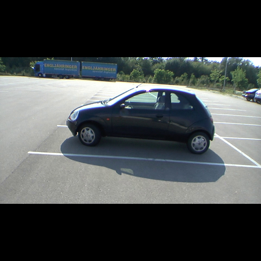
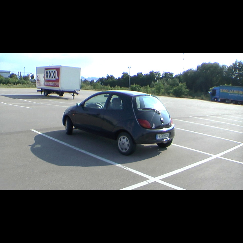
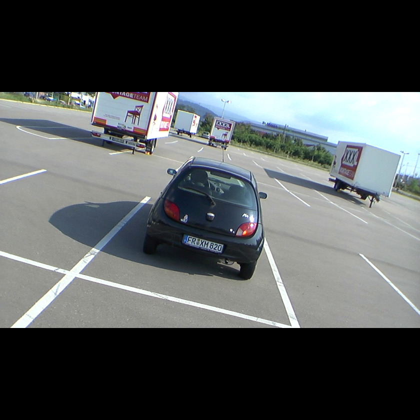
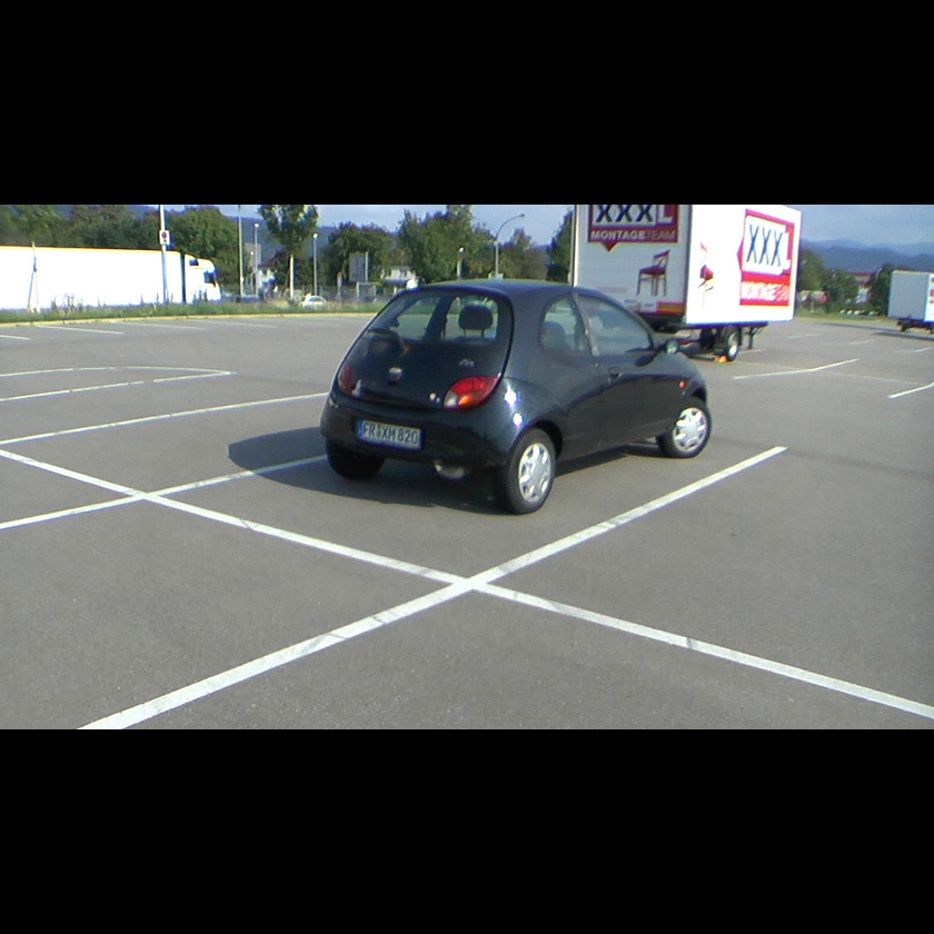
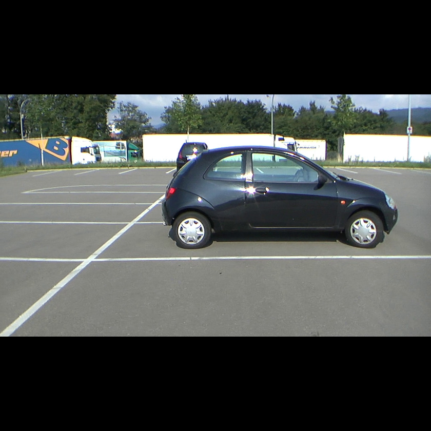
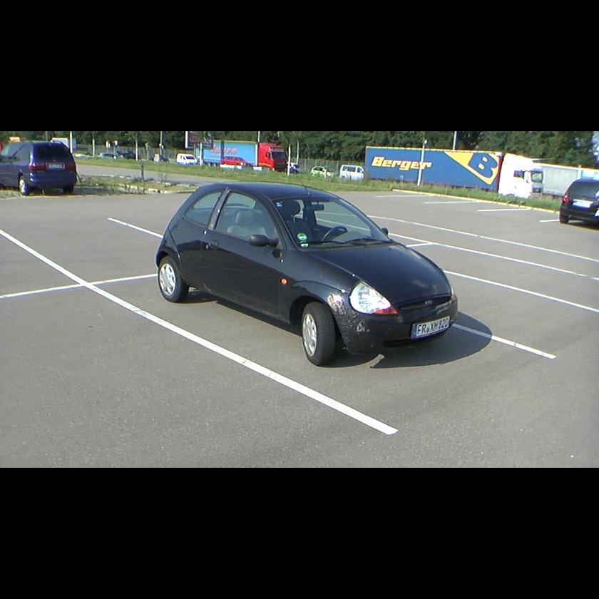
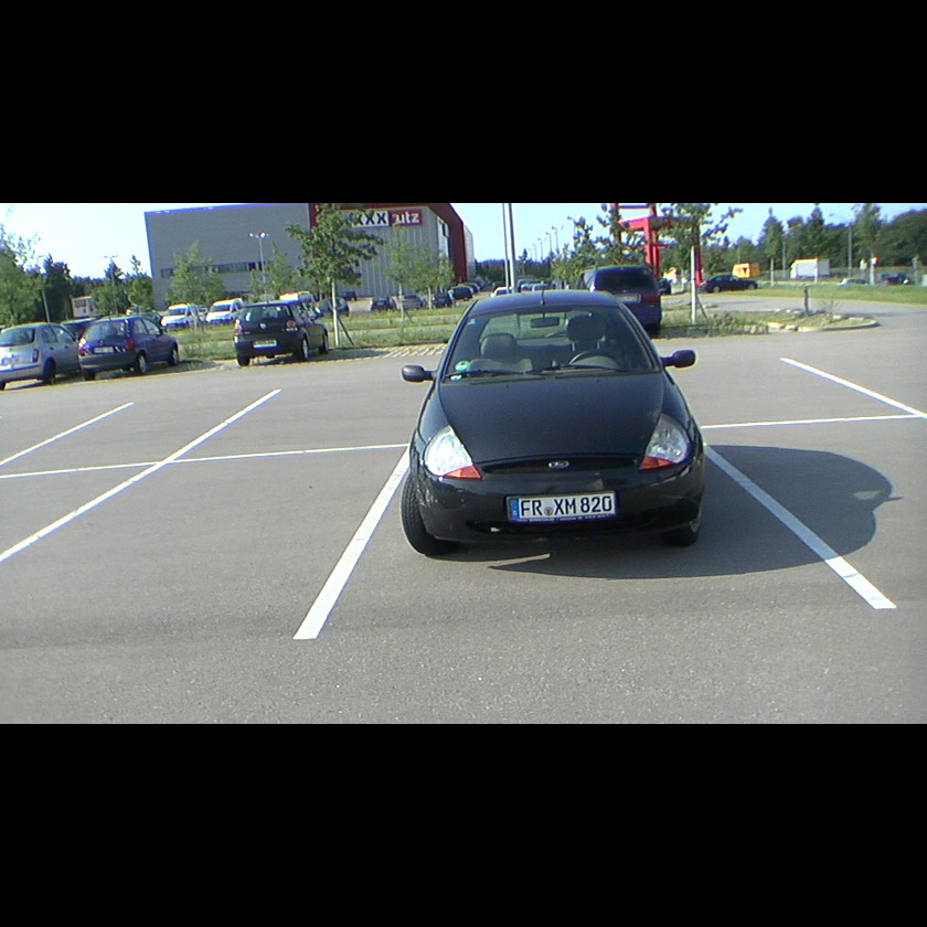
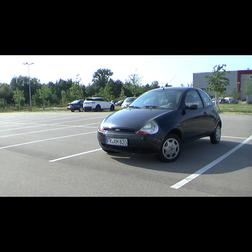
DINOv2
SD
DINOv2+SD
Sphere
Image
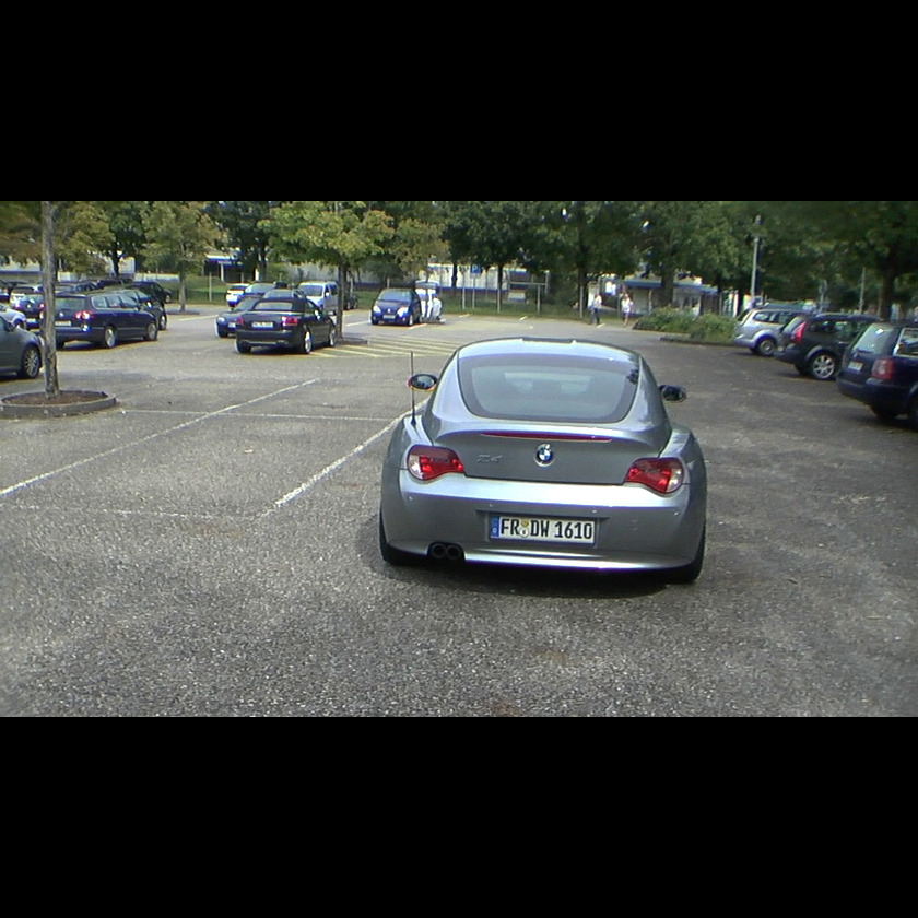
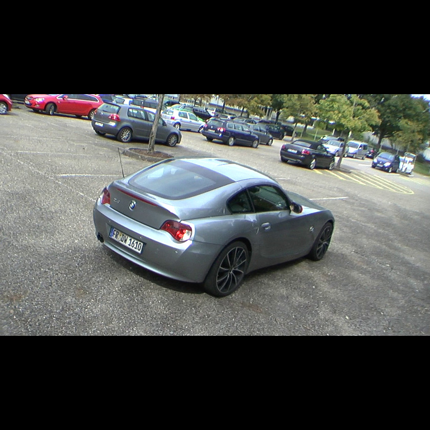
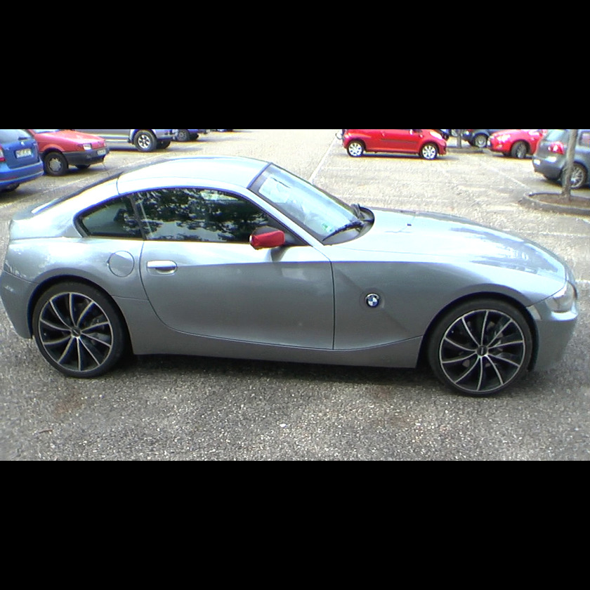
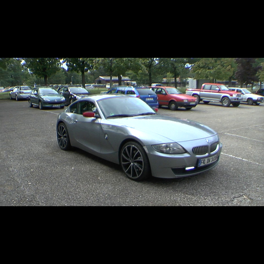
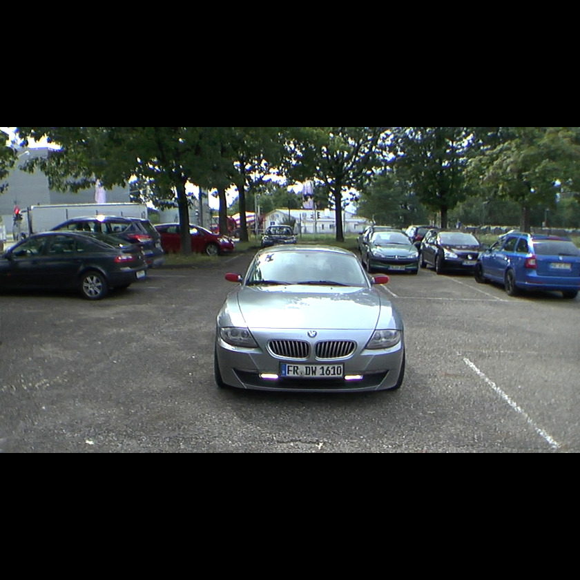
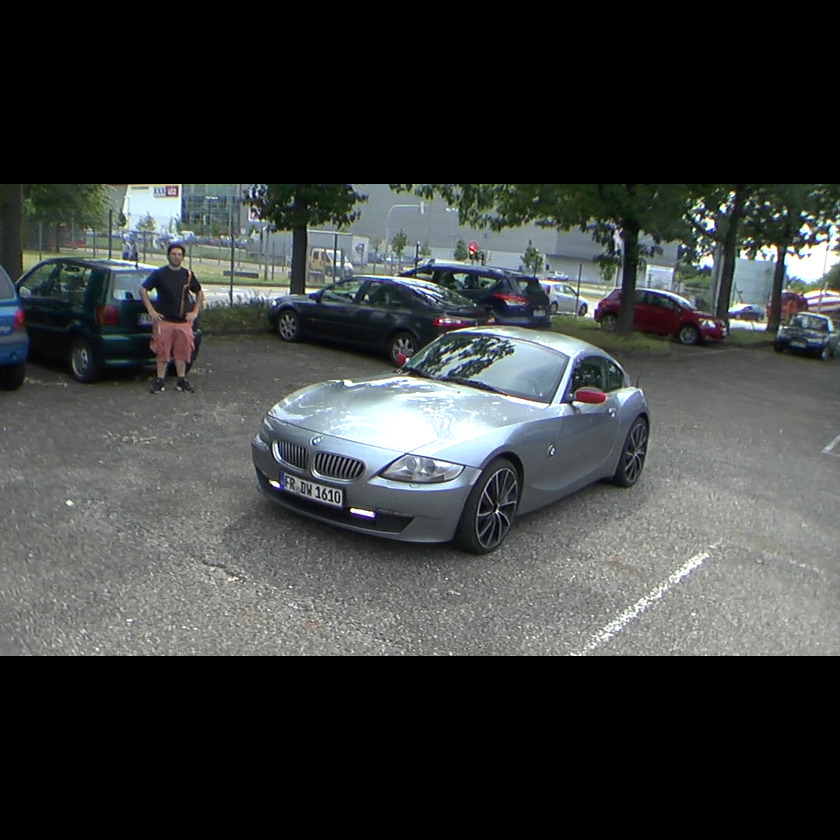
DINOv2
SD
DINOv2+SD
Sphere

Figure A1: Here we illustrate the multi-view consistency of our approach at test time on two different car sequences from the Freiburg cars dataset [44]. For each sequence, we show input images from different view points, DINOv2, Stable Diffusion (SD), and DINOv2+SD PCA feature maps, and our predicted spherical maps. While other models capture semantic parts, in contrast to us, they fail to correctly disambiguate the two different sides of each car resulting in the same features for the left and right sides. They also fail to produce distinct features for individual car wheels. Note, these large viewpoint changes are typically not assessed in the Spair-71k [34] benchmark. Please see the supplementary video for 360^∘ videos.

DINOv2
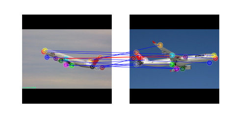
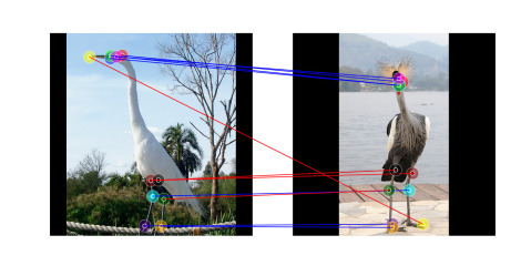
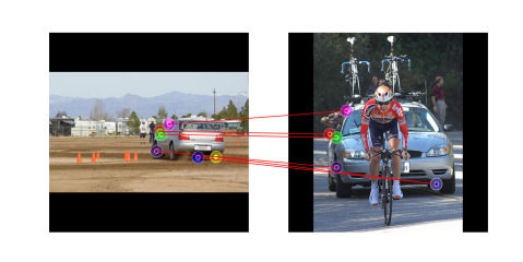
SD
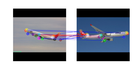
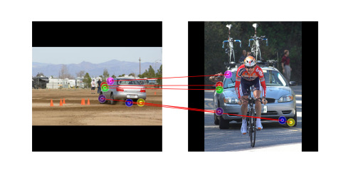
DINOv2+SD
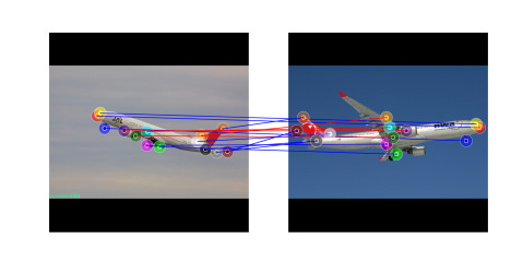
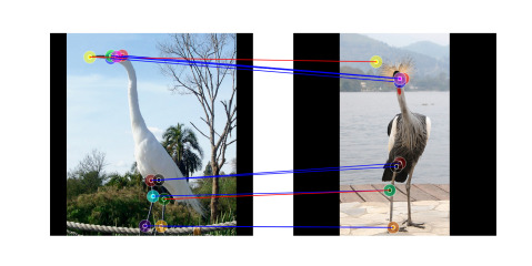
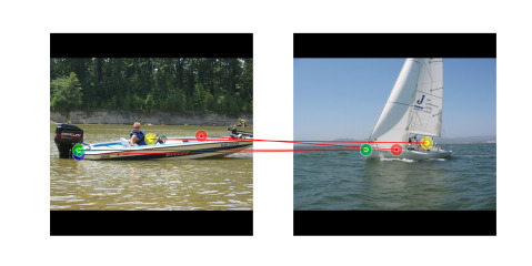
Ours
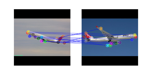
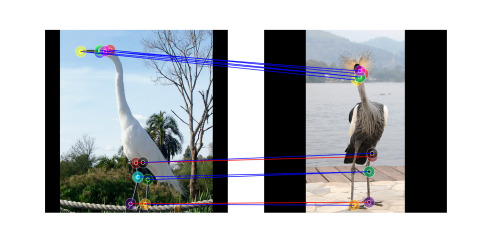
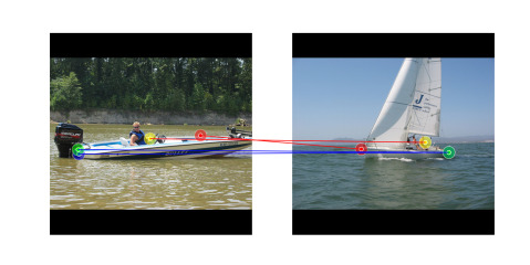
Ours+SD
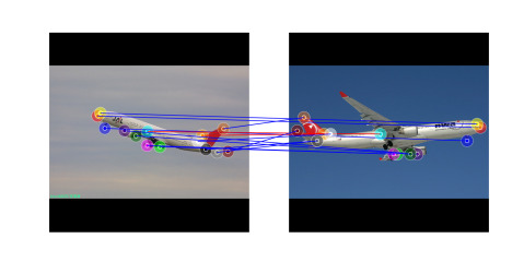
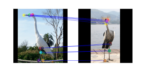
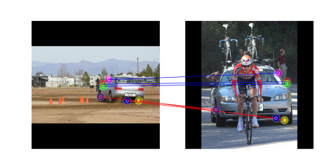
DINOv2
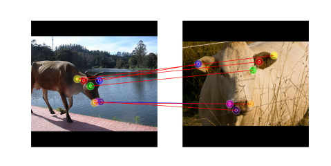
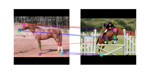
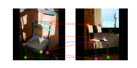
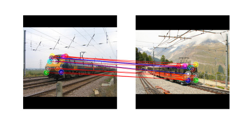
SD
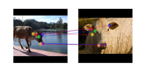
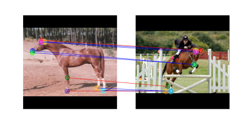
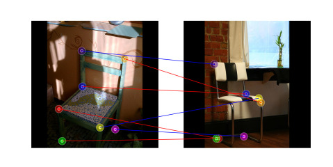
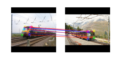
DINOv2+SD
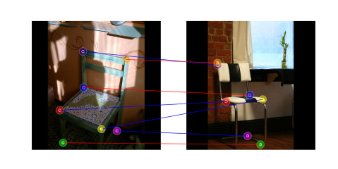
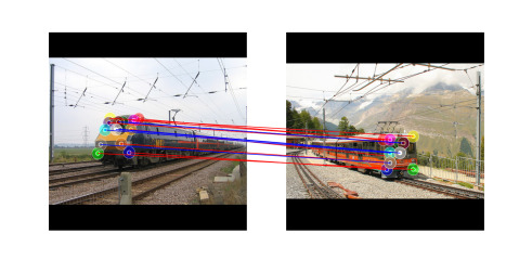
Ours
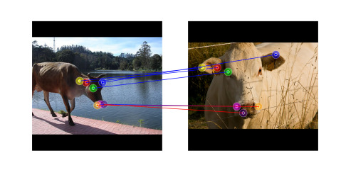
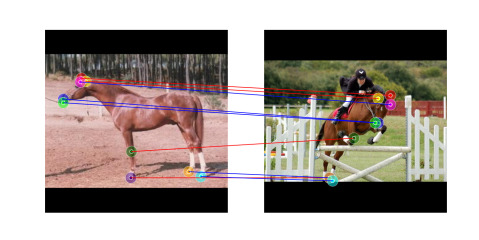
Ours+SD

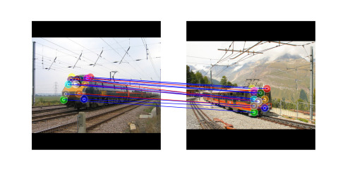
Figure A2: Keypoint matching on SPair-71k [34]. In each pair, the left image acts as the source, from which keypoint features are sampled, then the nearest neighbor of each feature is compute on the target to its right.

Image
DINOv2
SD
DINOv2+SD
Sphere

Figure A3: Example dense correspondence maps for categories from the SPair-71k [34] dataset.

References

- Amir et al. [2022] Shir Amir, Yossi Gandelsman, Shai Bagon, and Tali Dekel. Deep vit features as dense visual descriptors. ECCV Workshop - What is Motion For?, 2022.
- Aygün and Mac Aodha [2022] Mehmet Aygün and Oisin Mac Aodha. Demystifying unsupervised semantic correspondence estimation. In ECCV, 2022.
- Aygün and Mac Aodha [2023] Mehmet Aygün and Oisin Mac Aodha. SAOR: Single-View Articulated Object Reconstruction. arXiv:2303.13514, 2023.
- Banik et al. [2021] Prianka Banik, Lin Li, and Xishuang Dong. A novel dataset for keypoint detection of quadruped animals from images. arXiv:2108.13958, 2021.
- Beauchemin and Barron [1995] Steven S. Beauchemin and John L. Barron. The computation of optical flow. ACM computing surveys, 1995.
- Caron et al. [2021] Mathilde Caron, Hugo Touvron, Ishan Misra, Hervé Jégou, Julien Mairal, Piotr Bojanowski, and Armand Joulin. Emerging properties in self-supervised vision transformers. In ICCV, 2021.
- Chen et al. [2013] Zhuoyuan Chen, Hailin Jin, Zhe Lin, Scott Cohen, and Ying Wu. Large displacement optical flow from nearest neighbor fields. In CVPR, 2013.
- Cheng et al. [2021] An-Chieh Cheng, Xueting Li, Min Sun, Ming-Hsuan Yang, and Sifei Liu. Learning 3d dense correspondence via canonical point autoencoder. NeurIPS, 2021.
- Cho et al. [2021] Seokju Cho, Sunghwan Hong, Sangryul Jeon, Yunsung Lee, Kwanghoon Sohn, and Seungryong Kim. Cats: Cost aggregation transformers for visual correspondence. NeurIPS, 2021.
- Choy et al. [2016] Christopher B Choy, JunYoung Gwak, Silvio Savarese, and Manmohan Chandraker. Universal correspondence network. NeurIPS, 2016.
- Dalal and Triggs [2005] Navneet Dalal and Bill Triggs. Histograms of oriented gradients for human detection. In CVPR, 2005.
- Davison et al. [2007] Andrew J Davison, Ian D Reid, Nicholas D Molton, and Olivier Stasse. Monoslam: Real-time single camera slam. PAMI, 2007.
- Dosovitskiy et al. [2021] Alexey Dosovitskiy, Lucas Beyer, Alexander Kolesnikov, Dirk Weissenborn, Xiaohua Zhai, Thomas Unterthiner, Mostafa Dehghani, Matthias Minderer, Georg Heigold, Sylvain Gelly, et al. An image is worth 16x16 words: Transformers for image recognition at scale. In ICLR, 2021.
- Ferrari et al. [2006] Vittorio Ferrari, Tinne Tuytelaars, and Luc Van Gool. Simultaneous object recognition and segmentation from single or multiple model views. IJCV, 2006.
- Goel et al. [2020] Shubham Goel, Angjoo Kanazawa, and Jitendra Malik. Shape and viewpoint without keypoints. In ECCV, 2020.
- Gupta et al. [2023] Kamal Gupta, Varun Jampani, Carlos Esteves, Abhinav Shrivastava, Ameesh Makadia, Noah Snavely, and Abhishek Kar. Asic: Aligning sparse in-the-wild image collections. In ICCV, 2023.
- Ham et al. [2017] Bumsub Ham, Minsu Cho, Cordelia Schmid, and Jean Ponce. Proposal flow: Semantic correspondences from object proposals. PAMI, 2017.
- Han et al. [2017] Kai Han, Rafael S Rezende, Bumsub Ham, Kwan-Yee K Wong, Minsu Cho, Cordelia Schmid, and Jean Ponce. Scnet: Learning semantic correspondence. In ICCV, 2017.
- Harris and Pike [1988] Christopher G Harris and JM Pike. 3d positional integration from image sequences. Image and Vision Computing, 1988.
- Hartley and Zisserman [2003] Richard Hartley and Andrew Zisserman. Multiple view geometry in computer vision. Cambridge university press, 2003.
- He et al. [2017] Kaiming He, Georgia Gkioxari, Piotr Dollár, and Ross Girshick. Mask r-cnn. In ICCV, 2017.
- Hedlin et al. [2023] Eric Hedlin, Gopal Sharma, Shweta Mahajan, Hossam Isack, Abhishek Kar, Andrea Tagliasacchi, and Kwang Moo Yi. Unsupervised semantic correspondence using stable diffusion. In NeurIPS, 2023.
- Henderson and Ferrari [2018] Paul Henderson and Vittorio Ferrari. Learning to generate and reconstruct 3d meshes with only 2d supervision. In BMVC, 2018.
- Hirschmuller [2005] Heiko Hirschmuller. Accurate and efficient stereo processing by semi-global matching and mutual information. In CVPR, 2005.
- Hu et al. [2021] Tao Hu, Liwei Wang, Xiaogang Xu, Shu Liu, and Jiaya Jia. Self-supervised 3d mesh reconstruction from single images. In CVPR, 2021.
- Huang et al. [2022] Shuaiyi Huang, Luyu Yang, Bo He, Songyang Zhang, Xuming He, and Abhinav Shrivastava. Learning semantic correspondence with sparse annotations. In ECCV, 2022.
- Jakab et al. [2018] Tomas Jakab, Ankush Gupta, Hakan Bilen, and Andrea Vedaldi. Unsupervised learning of object landmarks through conditional image generation. NeurIPS, 2018.
- Kingma and Ba [2015] Diederik P Kingma and Jimmy Ba. Adam: A method for stochastic optimization. In ICLR, 2015.
- Kulkarni et al. [2019] Nilesh Kulkarni, Abhinav Gupta, and Shubham Tulsiani. Canonical surface mapping via geometric cycle consistency. In ICCV, 2019.
- Liu et al. [2008] Ce Liu, Jenny Yuen, Antonio Torralba, Josef Sivic, and William T Freeman. Sift flow: Dense correspondence across different scenes. In ECCV, 2008.
- Long et al. [2014] Jonathan L Long, Ning Zhang, and Trevor Darrell. Do convnets learn correspondence? NeurIPS, 2014.
- Lowe [1999] David G Lowe. Object recognition from local scale-invariant features. In ICCV, 1999.
- Lowe [2004] David G Lowe. Distinctive image features from scale-invariant keypoints. IJCV, 2004.
- Min et al. [2019] Juhong Min, Jongmin Lee, Jean Ponce, and Minsu Cho. Spair-71k: A large-scale benchmark for semantic correspondence. arXiv:1908.10543, 2019.
- Min et al. [2020] Juhong Min, Jongmin Lee, Jean Ponce, and Minsu Cho. Learning to compose hypercolumns for visual correspondence. In ECCV, 2020.
- Monnier et al. [2022] Tom Monnier, Matthew Fisher, Alexei A Efros, and Mathieu Aubry. Share with thy neighbors: Single-view reconstruction by cross-instance consistency. In ECCV, 2022.
- Nishihara [1984] H K Nishihara. Prism: A practical realtime imaging stereo matcher. In Intelligent Robots: 3rd International Conference on Robot Vision and Sensory Controls, 1984.
- Ofri-Amar et al. [2023] Dolev Ofri-Amar, Michal Geyer, Yoni Kasten, and Tali Dekel. Neural congealing: Aligning images to a joint semantic atlas. In CVPR, 2023.
- Oquab et al. [2023] Maxime Oquab, Timothée Darcet, Théo Moutakanni, Huy Vo, Marc Szafraniec, Vasil Khalidov, Pierre Fernandez, Daniel Haziza, Francisco Massa, Alaaeldin El-Nouby, et al. Dinov2: Learning robust visual features without supervision. arXiv:2304.07193, 2023.
- Rocco et al. [2018] Ignacio Rocco, Mircea Cimpoi, Relja Arandjelović, Akihiko Torii, Tomas Pajdla, and Josef Sivic. Neighbourhood consensus networks. NeurIPS, 2018.
- Rombach et al. [2022] Robin Rombach, Andreas Blattmann, Dominik Lorenz, Patrick Esser, and Björn Ommer. High-resolution image synthesis with latent diffusion models. In CVPR, 2022.
- Rublee et al. [2011] Ethan Rublee, Vincent Rabaud, Kurt Konolige, and Gary Bradski. Orb: An efficient alternative to sift or surf. In ICCV, 2011.
- Schonberger and Frahm [2016] Johannes L Schonberger and Jan-Michael Frahm. Structure-from-motion revisited. In CVPR, 2016.
- Sedaghat and Brox [2015] Nima Sedaghat and Thomas Brox. Unsupervised generation of a viewpoint annotated car dataset from videos. In ICCV, 2015.
- Shapovalov et al. [2021] Roman Shapovalov, David Novotny, Benjamin Graham, Patrick Labatut, and Andrea Vedaldi. Densepose 3d: Lifting canonical surface maps of articulated objects to the third dimension. In ICCV, 2021.
- Shtedritski et al. [2023] Aleksandar Shtedritski, Andrea Vedaldi, and Christian Rupprecht. Learning universal semantic correspondences with no supervision and automatic data curation. In ICCV Workshops, 2023.
- Suwajanakorn et al. [2018] Supasorn Suwajanakorn, Noah Snavely, Jonathan J Tompson, and Mohammad Norouzi. Discovery of latent 3d keypoints via end-to-end geometric reasoning. NeurIPS, 2018.
- Tang et al. [2023] Luming Tang, Menglin Jia, Qianqian Wang, Cheng Perng Phoo, and Bharath Hariharan. Emergent correspondence from image diffusion. arXiv preprint arXiv:2306.03881, 2023.
- Taniai et al. [2016] Tatsunori Taniai, Sudipta N Sinha, and Yoichi Sato. Joint recovery of dense correspondence and cosegmentation in two images. In CVPR, 2016.
- Thewlis et al. [2017] James Thewlis, Hakan Bilen, and Andrea Vedaldi. Unsupervised learning of object frames by dense equivariant image labelling. NeurIPS, 2017.
- Thewlis et al. [2019] James Thewlis, Samuel Albanie, Hakan Bilen, and Andrea Vedaldi. Unsupervised learning of landmarks by descriptor vector exchange. In ICCV, 2019.
- Torr and Zisserman [1999] Philip HS Torr and Andrew Zisserman. Feature based methods for structure and motion estimation. In International workshop on vision algorithms, 1999.
- Ufer and Ommer [2017] Nikolai Ufer and Bjorn Ommer. Deep semantic feature matching. In CVPR, 2017.
- Walmer et al. [2023] Matthew Walmer, Saksham Suri, Kamal Gupta, and Abhinav Shrivastava. Teaching matters: Investigating the role of supervision in vision transformers. In CVPR, 2023.
- Wu et al. [2023] Shangzhe Wu, Ruining Li, Tomas Jakab, Christian Rupprecht, and Andrea Vedaldi. MagicPony: Learning articulated 3d animals in the wild. In ICCV, 2023.
- Yen-Chen et al. [2022] Lin Yen-Chen, Pete Florence, Jonathan T Barron, Tsung-Yi Lin, Alberto Rodriguez, and Phillip Isola. Nerf-supervision: Learning dense object descriptors from neural radiance fields. In ICRA, 2022.
- Zhang et al. [2023] Junyi Zhang, Charles Herrmann, Junhwa Hur, Luisa Polania Cabrera, Varun Jampani, Deqing Sun, and Ming-Hsuan Yang. A tale of two features: Stable diffusion complements dino for zero-shot semantic correspondence. In NeurIPS, 2023.
- Zhao et al. [2021] Dongyang Zhao, Ziyang Song, Zhenghao Ji, Gangming Zhao, Weifeng Ge, and Yizhou Yu. Multi-scale matching networks for semantic correspondence. In ICCV, 2021.
- Zhou et al. [2022] Jinghao Zhou, Chen Wei, Huiyu Wang, Wei Shen, Cihang Xie, Alan Yuille, and Tao Kong. ibot: Image bert pre-training with online tokenizer. In ICLR, 2022.
- Zhou et al. [2015] Tinghui Zhou, Yong Jae Lee, Stella X Yu, and Alyosha A Efros. Flowweb: Joint image set alignment by weaving consistent, pixel-wise correspondences. In CVPR, 2015.
- Zhou et al. [2016] Tinghui Zhou, Philipp Krahenbuhl, Mathieu Aubry, Qixing Huang, and Alexei A Efros. Learning dense correspondence via 3d-guided cycle consistency. In CVPR, 2016.