Polylogarithmic-depth controlled-NOT gates without ancilla qubits

Abstract

Controlled operations are fundamental building blocks of quantum algorithms. Decomposing $n$-control-NOT gates ($C^{n}(X)$) into arbitrary single-qubit and CNOT gates, is a crucial but non-trivial task. This study introduces $C^{n}(X)$ circuits outperforming previous methods in the asymptotic and non-asymptotic regimes. Three distinct decompositions are presented: an exact one using one borrowed ancilla with a circuit depth $\Theta\left(\log(n)^{3}\right)$, an approximating one without ancilla qubits with a circuit depth $\mathcal{O}\left(\log(n)^{3}\log(1/\epsilon)\right)$ and an exact one with an adjustable-depth circuit which decreases with the number $m\leq n$ of ancilla qubits available as $\mathcal{O}\left(\log(n/\lfloor m/2\rfloor)^{3}+\log(\lfloor m/2\rfloor)\right)$. The resulting exponential speedup is likely to have a substantial impact on fault-tolerant quantum computing by improving the complexities of countless quantum algorithms with applications ranging from quantum chemistry to physics, finance and quantum machine learning.

I Introduction

In the past three decades, quantum algorithms promising an exponential speedup over their classical counterparts have been designed [1, 2, 3]. The advantages of these algorithms stem from the peculiar properties of superposition and entanglement of the quantum bits (qubits). These properties enable to manipulate a vast vector of qubit states using basic operations that act on either one or two qubits [3]. The question of decomposing efficiently any $n$-qubit operation into a reasonable number of primitive single- and two-qubit operations is one of the major challenges in quantum computing [4]. In this context, multi-controlled operations act as building-blocks of many prevalent quantum algorithms such as qubitisation [5] within the quantum singular value transformation [6], which have immediate repercussions on Hamiltonian simulation [7], quantum search [6] and quantum phase estimation methods [8]. For this reason, achieving more effective decompositions of multi-controlled operations has the potential to bring about significant enhancements in quantum algorithms, impacting various fields such as quantum chemistry, specifically in estimating ground state energy [9], physics for the simulation of quantum systems [10], engineering for solving partial differential equations [11, 12], quantum machine learning [13], and finance [14].
This non-trivial challenge and the quest for optimal solutions has been an active and ongoing research focus for decades. In 1995, Barenco et al. [15] proposed several linear depth constructions of multi-controlled NOT (MCX) gates (also known as $n$-Toffoli gates, multi-controlled Toffoli, generalised-Toffoli gates, multi-controlled $X$ or $n$-controlled NOT gates). All these linear depth constructions used ancilla qubits or relied on an efficient approximation, while the first ancilla-free exact decomposition has a quadratic depth.

Years later, exact implementations of controlled-NOT gates with linear depth and quadratic size were proposed [16, 17]. It is only in 2015 that Craig Gidney published a pedagogical blogpost describing an exact linear size decomposition without ancilla qubits [18]. Even though his method was linear, its depth leading coefficient is large compared to that of other methods. Still, this one-of-a-kind method was used in subsequent work [19, 20, 21]. In 2017, a logarithmic-depth controlled-NOT gate using as many zeroed ancilla qubits as control qubits was presented [22]. Such finding motivated the search for a trade-off between the number of ancillae and the circuit depth. Computational approaches have been implemented [23], suggesting that any zeroed ancilla qubit could be used to reduce the circuit depth of controlled operations. Recently, Orts et al. [24] provided a review of the 2022 state-of-the-art methods for MCX.

Every controlled-NOT decomposition method aims at optimising certain metrics such as circuit size, circuit depth, or ancilla count. This article considers only the case of $n$-controlled NOT gates with $n>2$. The attention is directed towards circuit depth, the metric associated to quantum algorithmic runtime, circuit size, the total number of primitive quantum gates, and ancilla qubit count, which corresponds to the amount of available qubits during the computation. A precise distinction is made between borrowed ancilla qubits (qubits in any state beforehand which are restored afterwards) and zeroed ancilla qubits (which are in state $\ket{0}$ initially and reset to $\ket{0}$ at the end of the computation). Zeroed ancilla qubits are efficient to use since they are initially in a well-known state. Borrowed ancilla qubits are more constraining but have the advantage to be available more often during computations: operations that do not impact the entire system can utilise unaffected wires as borrowed qubits.

This article introduces three novel circuit identities to build a $n$ control-qubit controlled-NOT gate $C^{n}(X)$. They display the following depth complexities.

1. Polylogarithmic-depth circuit with a single borrowed ancilla (Proposition 1).

2. Polylogarithmic-depth approximate circuit without ancilla (Proposition 5).

3. Adjustable-depth circuit using an arbitrary number $m\leq n$ of ancillae (Proposition 9).

The first one is an exact decomposition whose depth is affine in the depth of a quadratically smaller controlled operation $C^{\sqrt{n}}(X)$. The global decomposition takes advantage of a single borrowed ancilla qubit, and each of the smaller controlled operations can be associated to a locally borrowed ancilla. As a consequence, a new recursive construction of the controlled-NOT gate emerges with an overall polylogarithmic circuit depth in the number of control qubits $\Theta\left(\log(n)^{3}\right)$ and a circuit size $\tilde{\Theta}(n)$. The second method approximates a $C^{n}(X)$ without ancilla qubits up to an error $\epsilon>0$ with a circuit depth $\mathcal{O}\left(\log(n)^{3}\log(1/\epsilon)\right)$ and a circuit size $\tilde{\mathcal{O}}(n\log(1/\epsilon))$. It makes use of the decomposition of a $n$-controlled $X$ gate into $(n-1)$-controlled unitaries, generating borrowed ancilla qubits that facilitate the application of the first method up to an error $\epsilon$. The last method provides an adjustable-depth quantum circuit which implements exactly a $C^{n}(X)$ for any given number $m\leq n$ of zeroed ancilla qubits. The depth decreases with $m$ from a polylogarithmic-with-$n$ scaling to a logarithmic one as $\mathcal{O}\left(\log(n/\lfloor m/2\rfloor)^{3}+\log(\lfloor m/2\rfloor)\right)$. To the best of our knowledge, these new methods stand out as the only approaches achieving such depth complexities. In particular, they demonstrate an exponential speedup over previous state-of-the-art, and readily improves a wide range of quantum algorithms.

Section II introduces the three new methods and their asymptotic complexity scalings. Section III provides numerical simulations proving that the proposed methods are already of interest in the non-asymptotic regime when compared to other previous decompositions. Section IV discusses the advantages of this new methods for different prevalent quantum algorithms.

II Results

This section is subdivided into three parts. The first subsection details the logical steps towards achieving method 1. This includes a detailed study of the single-zeroed-ancilla case II.1.1, how it can be turned into a borrowed one in II.1.2 and where the recursive decomposition can stem from to yield the polylogarithmic-depth controlled-NOT circuit with a single borrowed ancilla in II.1.3. The methods 5 and 9 are described respectively in II.2 and II.3.

Notations

This paragraph gathers the most important definitions that will be used throughout the article. Let $n\geq 1$ and let $\{\ket{x}\}_{x=0}^{2^{n}-1}$ be the computational basis of an $n$-qubit register $R$ and $T$ be a one-qubit register, the so-called target register. The $C^{n}(X)$ controlled by $R$ with target $T$ is the gate defined by equation 1:

$$C^{n}(X) =(I_{R}-\ket{2^{n}-1}\bra{2^{n}-1})\otimes I_{T}$$ (1)

$$+\ket{2^{n}-1}\bra{2^{n}-1}\otimes X,$$

where $I_{R}$ and $I_{T}$ are the identities on register $R$ and $T$. The symbol $X$ denotes the Pauli matrix $X=\ket{0}\bra{1}+\ket{1}\bra{0}$. More generally, a $C^{n}(U)$ gate will denote a controlled $U$ gate. If the register $R$ is in state $\ket{2^{n}-1}$, it will be termed as active. When one wants to emphasise the control and target registers, one will note $\mathcal{C}_{R}^{T}$. If $R^{\prime}$ is a second qubit register, define the (partial) white control $\mathcal{C}_{\overline{R}\cup R^{\prime}}^{T}\equiv\left(\prod_{q\in R}X_{q}\right)\mathcal{C}_{R\cup R^{\prime}}^{T}\left(\prod_{q\in R}X_{q}\right)$, where the label $q$ denotes the qubit on which the $X$ gate is performed. The support of a quantum circuit is the set of qubits on which it does not act like the identity. Ancilla qubits are qubits outside the support of $U$ which may be used during the computation. From now, the function $\log$ signifies the logarithm in base 2. All circuit sizes and depths are computed in the basis of arbitrary single-qubit and CNOT gates.

II.1 Polylogarithmic-depth decomposition of the $C^{n}(X)$ gate using one borrowed ancilla

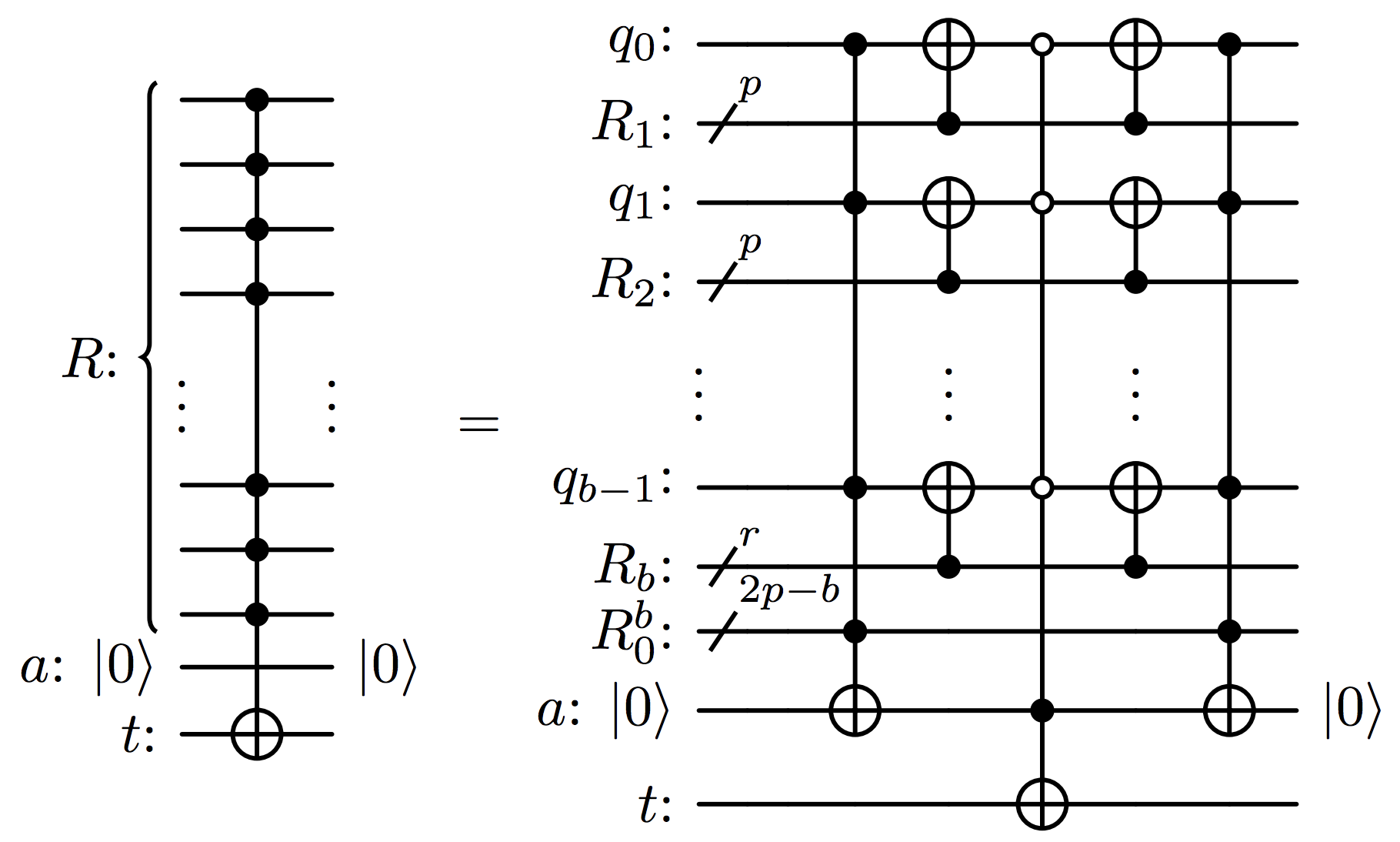
Figure 1: $n$ controlled $\mathcal{C}_{R}^{t}$ using the zeroed ancilla $a$, where $p=\lfloor\sqrt{n}\rfloor$ and $R_{i}$ is a register of at most $p$ qubits for each $i\in\{1,...,b\}$. $r$ is the remainder of the euclidean division of $\left|R\backslash R_{0}\right|=n-2p$ by $p$, $r=\left|R_{b}\right|$.

II.1.1 A new decomposition of the $C^{n}(X)$ gate using a single zeroed ancilla

The decomposition uses a single zeroed ancilla to reduce the global MCX gate to five layers, each exhibiting the depth of a quadratically smaller operation. The $n$-control-qubit register $R=\{q_{0},...,q_{n-1}\}$ is first divided into subregisters. Let $p=\lfloor\sqrt{n}\rfloor$. The control register $R$ can then be written as the disjoint union $R=\bigcup_{i=0}^{b}R_{i}$ where subregister $R_{0}=\{q_{0},...,q_{2p-1}\}$ is a subregister of size $2p$ and subregister $R_{i}$ is of size at most $p$, for each $i\in\{1,...,p\}$. More precisely, let $R_{i}=\{q_{j}\}_{j=(1+i)p}^{(2+i)p-1}$ for each $i\in\{0,...,p-1\}$. Let $b=|\{i\in\{1,...,p\}:R_{i}\neq\emptyset\}|$ be the number of non-empty registers of positive index. Moreover, the first register $R_{0}$ is further divided into $R_{0}^{*}=\{q_{i}\}_{i=0}^{b-1}$ containing the first $b$ qubits and $R_{0}^{b}=R_{0}\backslash R_{0}^{*}$.

The circuit in Figure 1 illustrates a decomposition of the controlled-NOT operation $\mathcal{C}_{R}^{t}$ using a single zeroed ancilla. Note that qubit $q_{i}$ is positioned between registers $R_{i}$ and $R_{i+1}$. The unitary associated to the circuit is given by

$$\mathcal{U}_{0}\equiv\mathcal{C}_{R_{0}}^{a}\mathfrak{C}\leavevmode\nobreak\ \mathcal{C}_{R_{0}}^{a},$$ (2)

where

$$\mathfrak{C}\leavevmode\nobreak\ \equiv\left(\prod_{i=1}^{b}\mathcal{C}_{R_{i}}^{q_{i-1}}\right)\mathcal{C}_{\overline{R_{0}^{*}}\cup{a}}^{t}\left(\prod_{i=1}^{b}\mathcal{C}_{R_{i}}^{q_{i-1}}\right).$$ (3)

The first operation $\mathcal{C}_{R_{0}}^{a}$ sets the zeroed ancilla to $\ket{1}$ if and only if $R_{0}$ is active. Now, consider the operation $\mathfrak{C}$: for $\mathcal{C}_{\overline{R_{0}^{*}}\cup{a}}^{t}$ to apply an $X$ gate to the target, all the qubits from $R_{0}^{*}$ must be in state $\ket{0}$, and the ancilla $a$ must be in state $\ket{1}$. Now, notice that for each qubit $q_{i}\in R_{0}^{*}$, $q_{i}$ is in state $\ket{0}$ when applying $C_{\overline{R_{0}^{*}}\cup{a}}^{t}$ if and only if it was in the same activation state as $R_{i+1}$ right before applying $\mathfrak{C}$. Therefore, $\mathfrak{C}$ is a multi-controlled-$X$ gate conditioned on:

• the ancilla $a$ being in state $\ket{1}$ and

• for each index $i\in\{0,...,b-1\}$: $q_{i}$ being in the same activation state as $R_{i+1}$.

By inspection, in the circuit in Figure 1, these conditions are fulfilled if and only if the register $R$ of interest is active. Therefore, the target $t$ is flipped under exactly the right hypothesis. The operations following the potential flip of qubit $t$ leave it unchanged and reset both the qubits from $R_{0}^{*}$ and the ancilla to their initial state. The overall operation is the desired $\mathcal{C}_{R}^{t}$ gate. A more formal proof is given in Appendix A.

II.1.2 Turning a zeroed ancilla into a borrowed one

This subsection discusses how the above zeroed ancilla is transformed into a borrowed ancilla. The construction is displayed in the circuit in Figure 2, which is formally defined by the unitary operation

$$\mathcal{U}\equiv\mathfrak{C}\leavevmode\nobreak\ \mathcal{C}_{R_{0}}^{a}\mathfrak{C}\leavevmode\nobreak\ \mathcal{C}_{R_{0}}^{a}=\mathfrak{C}\leavevmode\nobreak\ \mathcal{U}_{0}.$$ (4)

Notice that $\mathcal{U}_{0}$ and $\mathfrak{C}$ both leave the control qubits and the ancilla unchanged. As a consequence, one only needs to focus on what happens to the target $t$. If the ancilla starts in state $\ket{0}$, the last $\mathfrak{C}$ does not affect $t$ and $\mathcal{U}$ overall acts as the desired $\mathcal{C}_{R}^{t}$ gate . It is now sufficient to focus on the case where qubit $a$ arrives in state $\ket{1}$ and to repeat the above analysis: $\mathcal{U}_{0}$ flips the target if both $R_{0}$ is inactive and for each $i\in\{0,...,b-1\}$, qubit $q_{i}$ is in the same activation state as $R_{i+1}$. Refer to this flip as the first flip. Then, $\mathfrak{C}$ flips the target if and only if for each $i\in\{0,...,b-1\}$, qubit $q_{i}$ is in the same activation state as $R_{i+1}$. Refer to this flip as the second flip. Summarising, if $R$ is active only the second flip occurs. If $R$ is inactive, there are two cases: $R_{0}$ is either inactive or active. If $R_{0}$ is inactive, both flip 1 and flip 2 occur, resulting in no flip at all. If $R_{0}$ is active, the second condition cannot be verified. Therefore, none of the two flips occurs. In any case, the circuit applies the $\mathcal{C}_{R}^{t}$ gate and leaves the ancilla unaffected. A more thorough proof is given in appendix A.

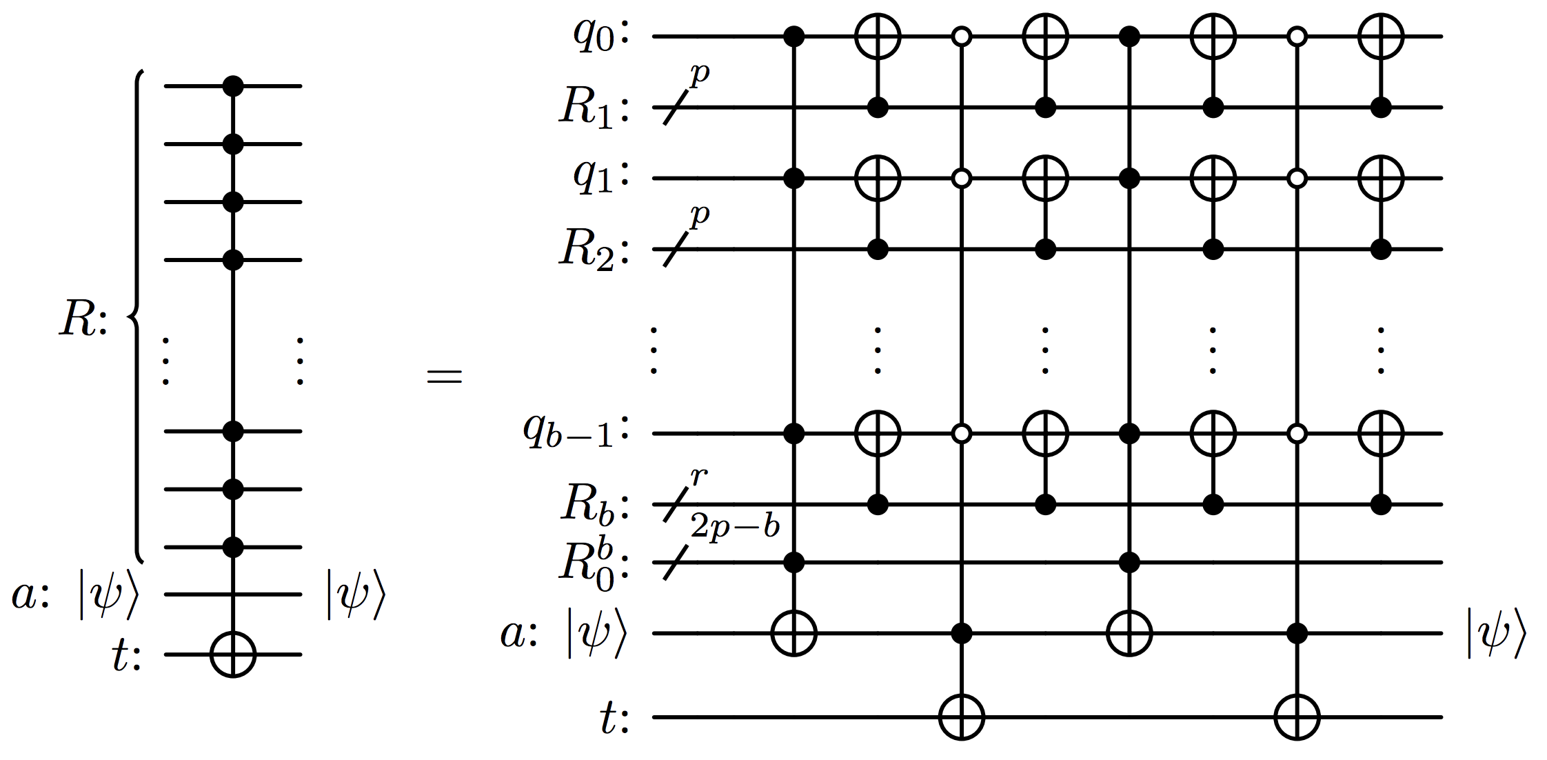
Figure 2: $n$ controlled $\mathcal{C}_{R}^{t}$ using the borrowed ancilla $a$, where $p=\lfloor\sqrt{n}\rfloor$ and $R_{i}$ is a register of at most $p$ qubits for each $i\in\{1,...,b\}$. $r$ is the remainder of the euclidean division of $\left|R\backslash R_{0}\right|=n-2p$ by $p$, $r=\left|R_{b}\right|$.

II.1.3 Recursive construction of the $C^{n}(X)$ gate

It is now possible to use a borrowed ancilla to implement any $C^{n}(X)$ using smaller $C^{2p}(X)$, $C^{p+1}$ and $C^{p}(X)$ gates. This section details how a qubit can be borrowed to compute each of the smaller MCX operations. This allows to set up a recursive construction, keeping the number of ancillae to one and achieving the polylogarithmic depth decomposition of $n$-MCX.

In Figure 2, the block $\displaystyle\prod_{i=1}^{b}\mathcal{C}_{R_{i}}^{q_{i-1}}$ has the same depth as a single controlled-NOT gate with $p$ control qubits since it is the product of $b$ unitaries with disjoint support. The depth of a controlled operation containing white controls is the same as that of standard controlled-NOT plus that of two additional layers of X gates acting on qubits whose control colour is white. One may want to apply the decomposition from the circuit in Figure 2 to each $C^{p}(X)$ gate. In order to do so, each block must have a borrowed ancilla qubit at its disposal.

There are more available borrowed qubits in the register $R_{0}^{b}$ than operations to perform in parallel: $\left|R_{0}^{b}\right|\geq\left|R_{0}^{*}\right|$ (see Appendix A). Hence, there are sufficiently many borrowed ancilla qubits to construct the smaller operations recursively. The recursion gives the following equality for the depth $D_{n}$ of a $C^{n}(X)$ gate.

$$D_{n}=2D_{2p}+4D_{p}+2D_{b+1}+4,$$ (5)

with $p=\lfloor\sqrt{n}\rfloor$ and $p-2\leq b\leq p$. The asymptotic behavior of the depth can be studied as follow: let $(D(k))_{k\in\mathbb{N}}\equiv\left(D_{2^{k+2}}\right)_{k\in\mathbb{N}}$ be the circuit depth of $C^{2^{k+2}}(X)$ gates. Equation 5 implies:

$$D(k)\leq 8D(k/2)+4.$$ (6)

The Master Theorem [28], recalled in Appendix B, implies that $D(k)\in\mathcal{O}\left(k^{3}\right)$. In terms of $n$, the circuit depth of a $C^{n}(X)$ gate using one borrowed ancilla qubit is $D_{n}\in\mathcal{O}\left(\log(n)^{3}\right)$. Now, a lower bound is derived by defining $\left(\tilde{D}(k)\right)_{k\in\mathbb{N}}\equiv\left(D_{2^{k}}\right)_{k\in\mathbb{N}}$ such that $\tilde{D}(k)\geq 8\tilde{D}(k/2)+4$. Similarly, this inequality leads to $D_{n}\in\Omega\left(\log(n)^{3}\right)$. The scaling of the size is computed similarly to the scaling of the depth, i.e. by solving the corresponding recursive equation. Details are given in Appendix C. The following proposition gathers these statements.

Proposition 1.

A controlled-NOT gate with $n$ control qubits is implementable with a circuit of depth $\Theta\left(\log(n)^{3}\right)$, size $\mathcal{O}\left(n\log(n)^{4}\right)$ and using a single borrowed ancilla qubit through the recursive use of circuit in Figure 2.

A first application improved by Proposition 1 affects the decomposition of multi-controlled unitary $C^{n}(U)$ using one zeroed ancilla. The zeroed ancilla allows to decomposed a $C^{n}(U)$ gate into two $C^{n}(X)$ gates and one $C^{1}(U)$ using the circuit identity in Figure 3 (Lemma 7.11 from [15]).

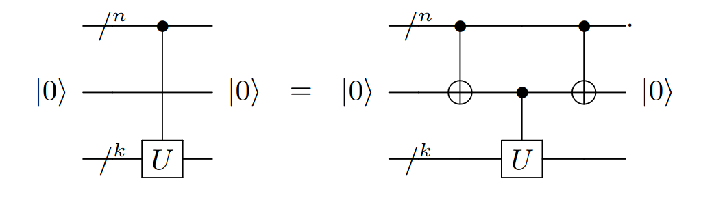
Figure 3: Controlling arbitrary unitary operation with a zeroed ancilla qubit.

The following corollary gives the complexity to implement a $C^{n}(U)$ gate.

Corollary 1.

Let $U$ be a unitary of size $S$ in the basis of single-qubit gates and CNOT gates. A controlled $U$ gate with $n$ control qubits is implementable with depth $\mathcal{O}\left(S+\log(n)^{3}\right)$, size $\mathcal{O}\left(S+n\log(n)^{4}\right)$ and one zeroed ancilla qubit through the circuit in Figure 3.

It is also straight-forward to implement any special unitary single-qubit gate $W\in\mathsf{SU}(2)$ with polylogarithmic complexity and without ancilla. This can be done with the help of Lemma 7.9 in [15], illustrated in Figure 4.

Corollary 2.

Let $W$ be a special unitary single-qubit gate. A $C^{n}(W)$ operation can be implemented with a circuit of depth $\mathcal{O}\left(\log(n)^{3}\right)$ and size $\mathcal{O}\left(n\log(n)^{4}\right)$ without ancilla qubits.

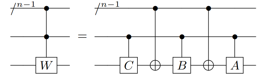
Figure 4: Controlling arbitrary special unitary operation $W$. Without loss of generality, $W=AXBXC$ for some matrices $A,B,C\in\mathsf{SU}(2)$ such that $ABC=I$.

II.2 Polylogarithmic-depth and ancilla-free approximate decomposition of the $C^{n}(X)$ gate

This section outlines how to make use of Proposition 1 to control single-qubit unitaries in the absence of ancilla qubits. The first step generates borrowed ancilla qubits by decomposing a $n$-controlled unitary into $(n-1)$-controlled unitaries. More precisely, for any single-qubit unitary $U$ whose square root is denoted by $V$, one can implement a $C^{n}(U)$ gate from two $C^{n-1}(X)$, a $C^{n-1}(V)$ and two simple two-qubit gates using the circuit identity in Figure 5 (Lemma 7.8 in [15]).

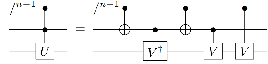
Figure 5: Decomposition of $n$-controlled unitary $U$ in terms of $(n-1)$-controlled gates and single-control gates.

Applying this decomposition $k$ times involves implementing the $2^{k}$-th root $V_{k}$ of the original unitary. Performing this recursion $n$ times leads to a linear depth quantum circuit [18]. To circumvent this issue, it is possible to neglect the $(n-k)$-controlled $V_{k}$ gate, introducing an error exponentially small with $k$ (Lemma 7.8 in [15]):

$$\left\|C^{n-k}(V_{k})-C^{n-k}(I)\right\|\leq\pi/2^{k}.$$ (7)

Applying the recursion $k=\lceil\log(\pi/\epsilon)\rceil$ times gives an $\epsilon>0$ error on the implementation of the $C^{n}(U)$ gates. This decomposition leads to $2k$ one-controlled-root of $U$ and $2k$ multi-controlled NOT gates. Each MCX gate is controlled by a number $j\in\{1,...,n-1\}$ of qubits and, therefore, is implementable using one of the non-affected qubit as a borrowed ancilla through the first method 1 with a polylogarithmic depth. The following proposition summarises the complexity of the method.

Proposition 2.

For any single-qubit unitary $U\in\mathsf{U}(2)$, a controlled-$U$ gate with $n$ control qubits is implementable up to an error $\epsilon>0$ with a circuit of depth $\mathcal{O}\left(\log(n)^{3}\log(1/\epsilon)\right)$, size $\mathcal{O}\left(n\log(n)^{4}\log(1/\epsilon)\right)$ without ancilla qubits.

The size and depth of the quantum circuits are trivially bounded noticing that the computational cost of $k$ $j$-MCX, $j\leq n-1$, is bounded by the computational cost of $k$ $n$-multi-controlled NOT gates.

This approximation proves highly effective for practical applications, as it is not needed to implement gates with exponentially small phases. The error $\epsilon>0$ can be selected to align with the intrinsic hardware error, providing a level of flexibility that exact methods approaches may not offer.

II.3 Adjustable-depth method

This subsection explains how to implement a $C^{n}(X)$ gate given $2\leq m\leq n$ zeroed ancilla qubits. For simplicity, consider an even number of ancillae $m$ and a number of control qubits $n$ divisible by $m/2$. The method has three steps: a first one where $m/2$ controlled-NOT gates, each controlled by $n/(m/2)$ qubits, are performed in parallel in order to store the activation of the subregisters into $m/2$ ancillae. A second step where a $C^{m/2}(X)$ controlled by the first $m/2$ ancillae is implemented on the target qubit using the last $m/2$ zeroed ancillae. A last one to restore the ancilla qubits in state $\ket{0}$. The first step makes use of Proposition 1 to implement each $C^{n/(m/2)}(X)$ with depth $\Theta\left(\log(n/(m/2))^{3}\right)$ using one zeroed ancilla of the last $m/2$ ancillae. The second step uses the logarithmic method from [22] to implement the $C^{m/2}(X)$ with depth $\mathcal{O}(\log(m/2))$ using $m/2$ ancillae. The circuit in Figure 6 represents the three steps of the adjustable-depth method.

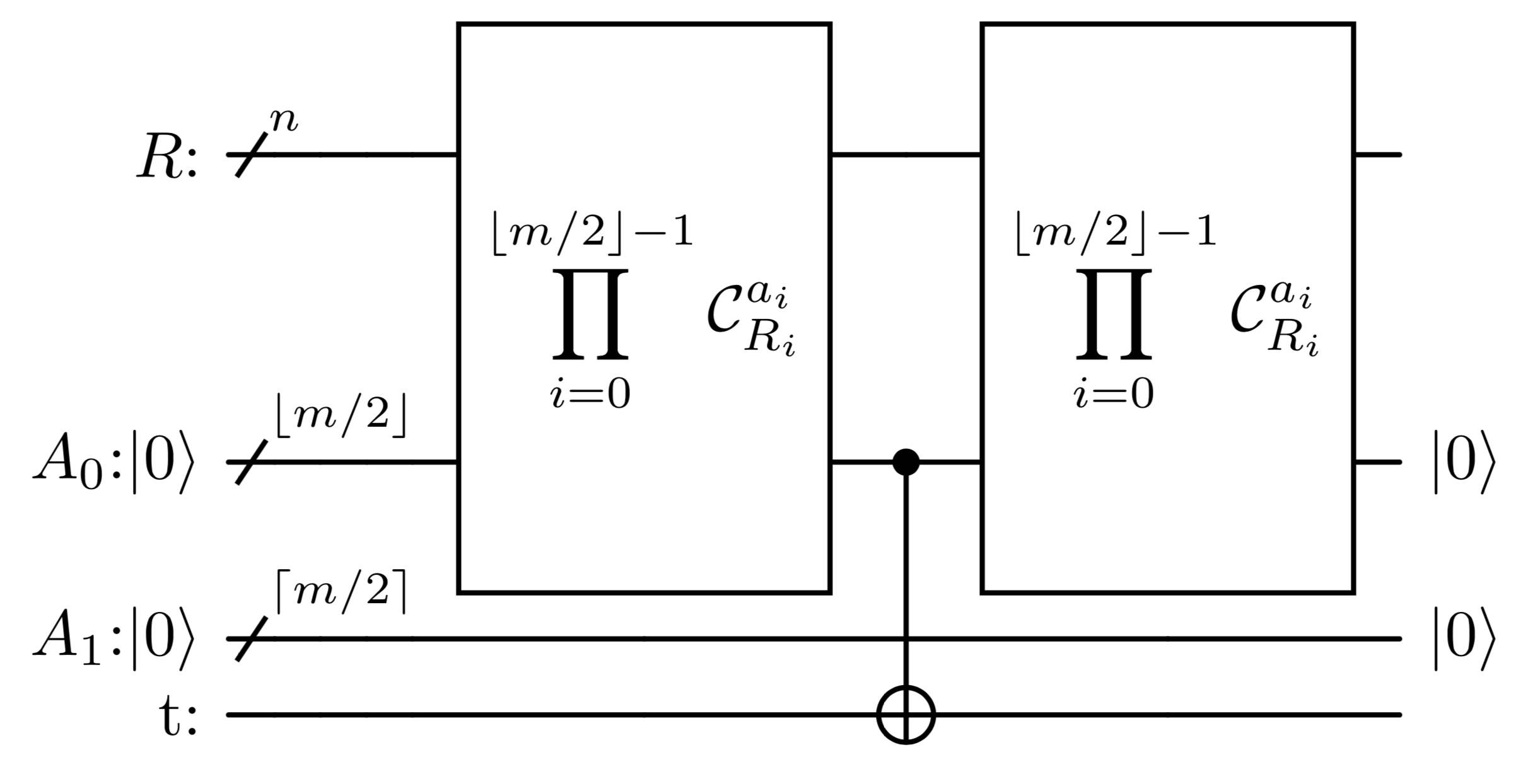
Figure 6: Adjustable-depth quantum circuit for $C^{n}(X)$ using an arbitrary number $m\in\{2,...,n\}$ of zeroed ancillae.

More generally, one can consider any value of $n$ control qubits and $m$ ancilla qubits such that $2\leq m\leq n$ qubits. Let $A=\{a_{0},...,a_{m-1}\}$ be the register of zeroed ancilla qubits, $A_{0}=\{a_{0},...,a_{\lfloor m/2\rfloor-1}\}$ and $A_{1}=\{a_{\lfloor m/2\rfloor},...,a_{m-1}\}$ such that $A=A_{0}\cup A_{1}$ and let the control register $R$ be divided into $\lfloor m/2\rfloor$ balanced subregisters $(R_{i})_{i=0}^{\lfloor m/2\rfloor-1}$. Let $\Pi$ be the operation associated to the first step:

$$\Pi\equiv\displaystyle\prod_{i=0}^{\lfloor m/2\rfloor-1}\mathcal{C}_{R_{i}}^{a_{i}}.$$ (8)

Each of the $C_{R_{i}}^{a_{i}}$ is implemented in parallel of the others using the circuit in Figure 1 with one zeroed ancilla of register $A_{1}$. Since all the $C_{R_{i}}^{a_{i}}$’s are performed in parallel, the operation $\Pi$ has the same depth as the maximum depth of the $\mathcal{C}_{R_{i}}^{a_{i}}$’s. After applying $\Pi$, one can implement $\mathcal{C}_{A_{0}}^{t}$ using the method from [22], which uses as many ancillae as control qubits to achieve a logarithmic depth. Therefore, one can implement $C_{A_{0}}^{t}$ with depth $16\lceil\log(\lfloor m/2\rfloor)\rceil+12$ using $A_{1}$ as a register of zeroed ancilla qubits (Corollary 2 in [22]). Finally, one can repeat $\Pi$ to fully reset the register $A$. Proposition 9 summarises the complexity of this new method.

Proposition 3.

Let $n\geq 2$ be the number of control qubits and $2\leq m\leq n$ be the number of available zeroed ancillae. Then, there exists a decomposition of the $C^{n}(X)$ into single-qubit gates and CNOT gates with depth complexity:

$$\mathcal{O}\left(\log(n/\lfloor m/2\rfloor)^{3}+\log(\lfloor m/2\rfloor)\right).$$ (9)

Note that the depth decreases as the number of ancillae $m$ increases, providing a method with adjustable depth. This is a valuable asset for aligning with the constraints of the hardware resources. Also, remark that the method from [22] has been used only for the second part of the algorithm. Using it in the first part would require a number of ancilla qubits proportional to the number of blocks, thus be potentially large. Different combinations of methods did not seem to lead to particular improvements in terms of depth or size. Overall, this decomposition provides a range of logarithmic-depth methods using less than $n$ ancillae, by considering $m(n)=\alpha n$, with $0<\alpha<1$, improving the decomposition proposed in [22].

III Numerical Analysis

In non-asymptotic regimes, pre-factors play a crucial role. This section employs graphical comparisons and complexity tables to fairly evaluate the overall effectiveness of current MCX decomposition methods.

In the case where only one zeroed borrowed ancilla qubit is available, a comparison is made with the one ancilla method from [15] as well as Craig Gidney’s ancilla-free method, and illustrated in Figure 7. In practice, the recurrence from Proposition 1 must be initialised. For a number of control qubits $n$ less than $30$, the $C^{n}(X)$ gate is implemented using Barenco et al.’s single-borrowed-ancilla method. This implementation provides shallower circuit for any number of control qubits. In that case, the asymptotic advantage of Proposition 1 becomes evident early in the process, making the method applicable across various regimes.

Next, in the absence of an ancilla qubit but allowing an approximation error $\epsilon>0$, a comparison is conducted against the state-of-the-art method outlined by Silva et al. [29], as depicted in Figure 7. Proposition 5 yields a shallower circuit than the method [29] as soon as $n\gtrsim 10^{5}$.

Finally, with a fixed number of control qubits set at $n=100$, Figure 8 illustrates the depth as a function of the number of ancillae. For a single ancilla, the use of circuit in Figure 1 already surpasses the state-of-the-art, and an increase in the number of zeroed ancillae rapidly reduces the overall circuit depth. Proposition 9 achieves the same depth as the previous best method but with a significantly lower number of ancillae, getting even larger as the number $n$ of control qubits increases as depicted in Figure 8 and in Figure 9.

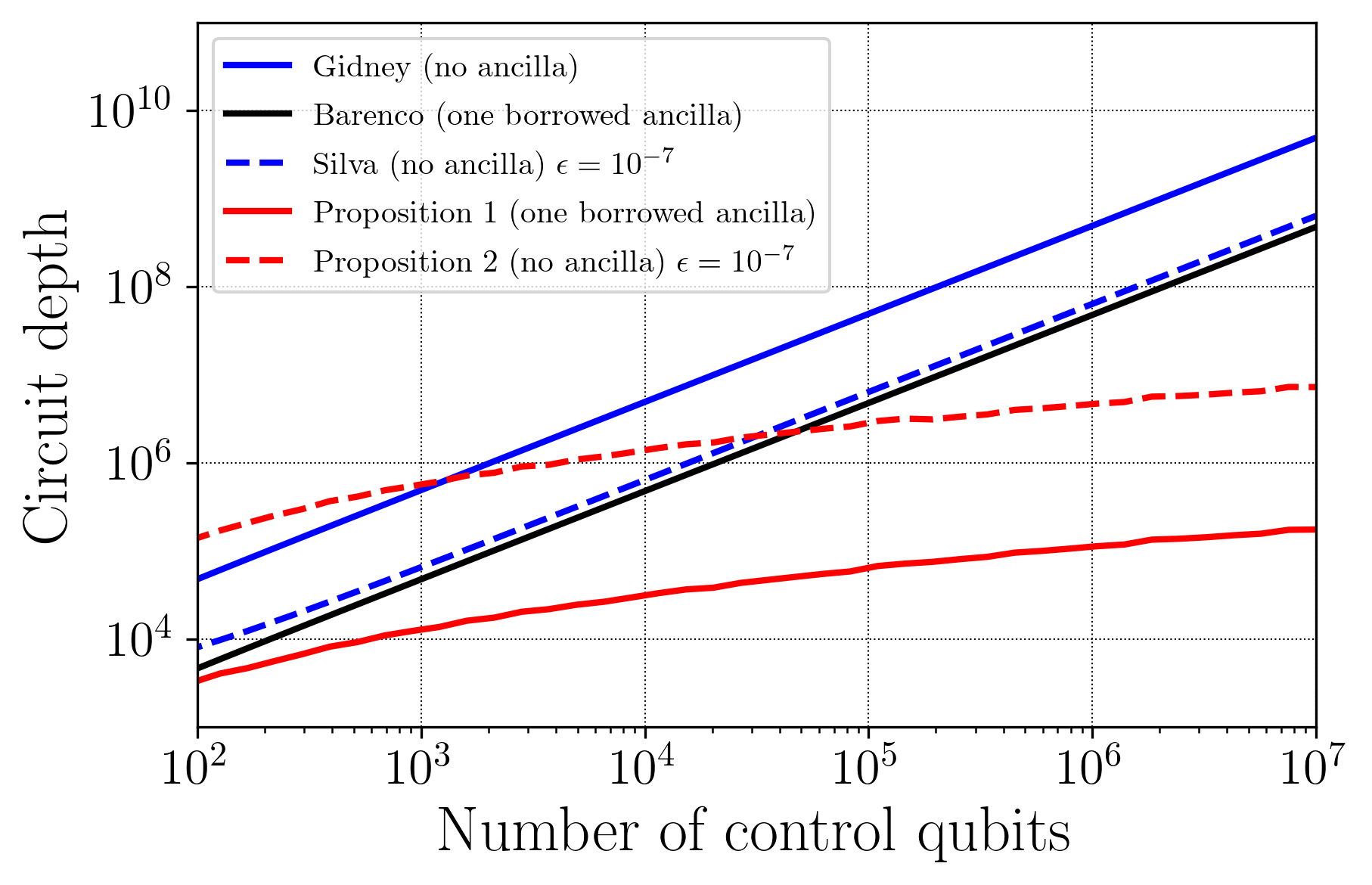
Figure 7: Comparison of circuit depths for methods involving a single or no ancilla.

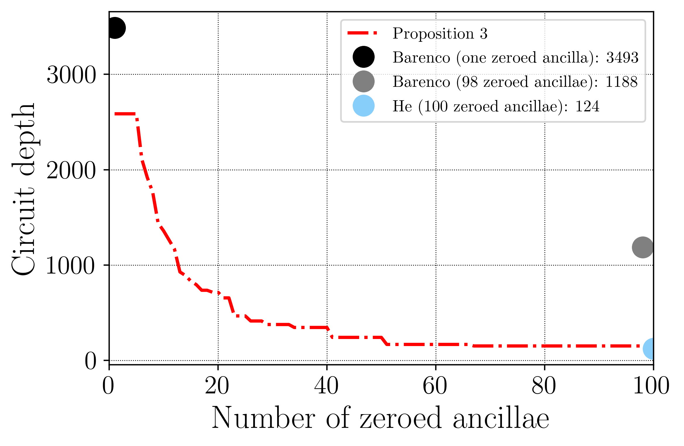
Figure 8: $C^{100}(X)$ as a function of the number of zeroed ancillae.

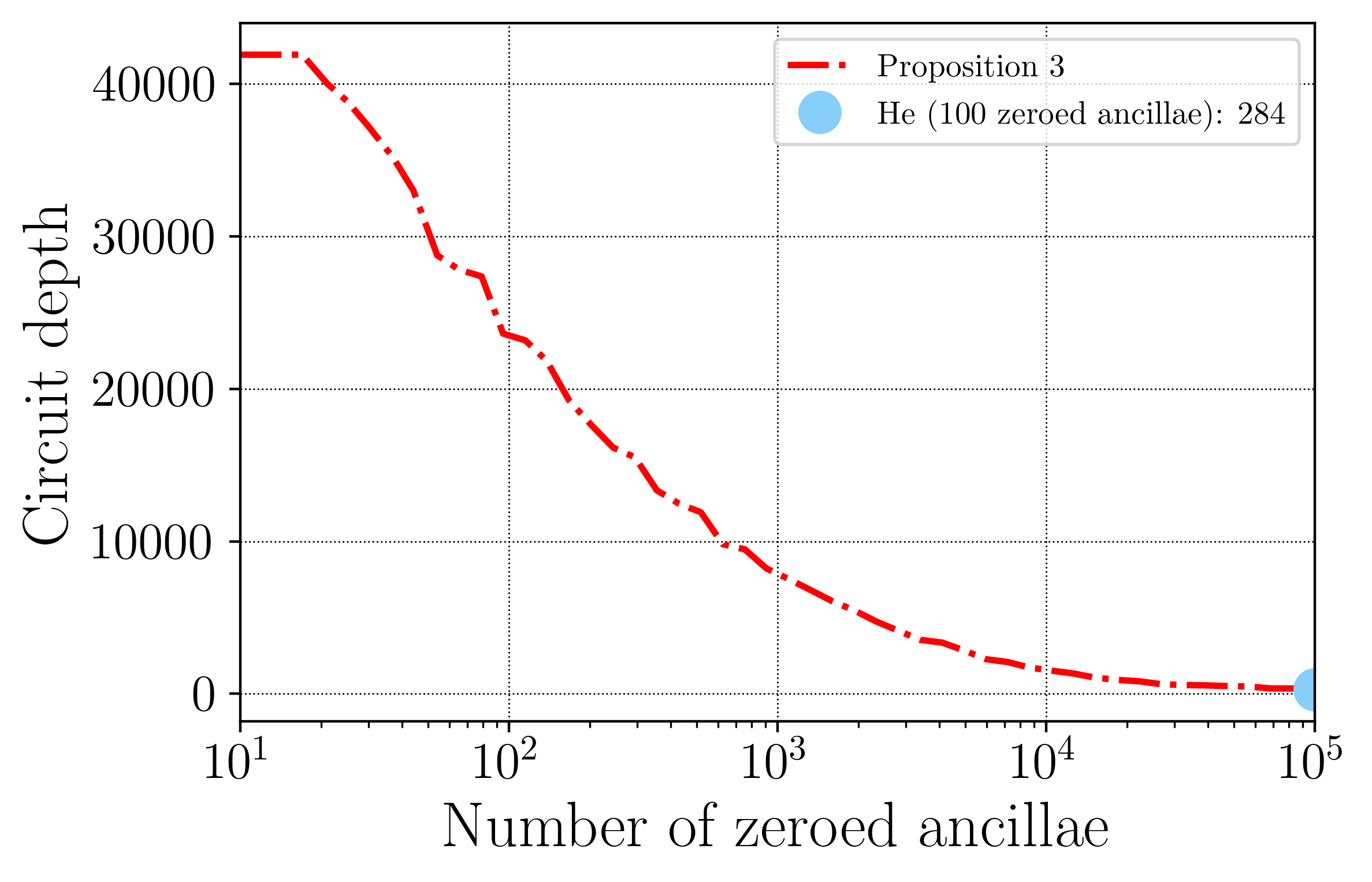
Figure 9: $C^{10^{5}}(X)$ as a function of the number of zeroed ancillae.

Table 3 compares the depth of various methods without employing any ancilla by fitting numerically the data from the implementations. Craig Gidney’s method stands out as the only exact method but results in a notably higher overall depth. The linear decomposition from [29] achieves a leading coefficient of $48$ at an approximation error of $\epsilon=10^{-7},$ representing a significant improvement. Lastly, the implementation of Proposition 5 delivers a depth of $\lceil\log(\pi/\epsilon)\rceil\left(43\log(n)^{3}-1287\right)$ and emerges as the most efficient method for $n\gtrsim 10^{5}$ control qubits.

In Table 3, various methods are compared when using a borrowed ancilla qubit. It is worth noting that employing such methods allows putting to use any qubit unaffected by the controlled operation for implementation, a situation frequently encountered in practice without the need for extra qubits. Notably, Proposition 1 is competitive across all control qubit numbers. The advantage becomes evident with over $10^{2}$ control qubits, resulting in a significant decrease in circuit depth.

Finally, Table 3 compares the methods using additional zeroed ancilla qubits. For a given number of available zeroed ancillae, Proposition 9 achieves shallower circuits. When the number of ancilla qubits matches the number of control qubits, the method proves as effective as the previously shallowest method by He et al. [22]. However, note that similar performances can be reached with significantly less zeroed ancillae (see Figure 8 and Figure 9).

Method	Scaling
Gidney [18]	$494n-1413$
Silva $(\epsilon)$[29]	$64n+1645$ if ($\epsilon=10^{-7}$)
Proposition 5 $(\epsilon)$	$\lceil\log(\pi/\epsilon)\rceil(86\log(n)^{3}-2564)$

Table 1: Circuit depth of ancilla-free methods.

Method	Scaling	Borrowed
Barenco 1 [15]	$48n-148$	1
Barenco $n-2$ [15]	$24n-43$	$n-2$
Proposition 1	$43\log(n)^{3}-1287$	1

Table 2: Circuit depth of borrowed ancillae methods.

Method	Scaling	Zeroed
Barenco 1 [15]	$36n-111$	1
Barenco $n-2$ [15]	$12n-12$	$n-2$
Proposition 1	$27\log(n)^{3}-808$	1
Proposition 9	$27\log(n/\lceil m/2\rceil)^{3}+$	$2\leq m\leq n$
	$16\lceil\log(\lfloor m/2\rfloor)\rceil-808$
He [22]	$16\lceil\log(n)\rceil+12$	$n$

Table 3: Circuit depth of zeroed ancillae methods^III.

IV Applications

This section provides an overview of some standard quantum algorithm oracles where multi-controlled operations act as both building blocks and complexity drivers, and where the improved decomposition reported in this paper readily provides the corresponding speedup.

Quantum search [30], quantum phase estimation [8], and Hamiltonian simulation [10] provide robust support for the claimed exponential quantum advantage. These algorithms can be seen as particular instances of the quantum singular value transformation (QSVT) [6], which allows the embedding of any Hamiltonian $H$ into an invariant subspace of the signal unitary, thereby enabling to compute a broad range of polynomials of $H$. The qubitisation [5] is the central technique to the framework of QSVT. When qubitising the Hamiltonian expressed as a linear combination $H=\sum_{k=1}^{s}\alpha_{k}U_{k}$, with each $U_{k}$ decomposable into a maximum of $C$ native gates, the process exhibits optimal query complexity for the two following oracles. The PREPARE oracle consists in a quantum state preparation step. Formally, it involves preparing the state $\ket{\text{PREPARE}}$ from a set of coefficients $\{\alpha_{k}\}_{k=1}^{s}$ such as :

$$\begin{split}\text{PREPARE}\ket{0}^{\otimes\log{s}}=\sum_{k=1}^{s}\sqrt{\frac{\alpha_{k}}{\lambda}}\ket{k},\lambda=\sum_{k=1}^{s}\alpha_{k}\end{split}$$ (10)

The CVO-QRAM algorithm [31] performs efficiently such task by proceeding $s$ layers of $n$-controlled operations, where $n$ represents the number of control qubits and $s$ represents the number of non-zero amplitude in the target state. The resulting circuit exhibits a depth of $\mathcal{O}(sn)$ assuming usual linear decomposition of multi-controlled operations. The $C^{n}(X)$ gate decompositions provided in this paper readily improves the scaling to $\mathcal{O}\left(s\log(n)^{3}\right)$. The PREPARE operator finds application in a broader context beyond qubitisation, whenever there is a need to transfer classical data into the qubit register. The SELECT oracle consists in a block-diagonal operator and acts as follows :

$$\text{SELECT}\equiv\sum_{k=1}^{s}\ket{k}\bra{k}\otimes U_{k}$$ (11)

It can be efficiently decomposed as $s$ layers of $\log(s)$-controlled-$U_{k}$ operations, yielding a depth in $\mathcal{O}\left(s\log(s)C\right)$ with usual linear-depth decomposition of $C^{\log(s)}(U)$ gates. The decompositions presented in this paper readily reduce the SELECT operation complexity to $\mathcal{O}\left(s\log(\log(s))^{3}C\right)$.

Considering an example application in ground-state quantum chemistry, the quantum phase estimation (QPE) stands as the standard fault-tolerant algorithm. The QPE performs a projection on an eigenstate of the Hamiltonian and provides an estimate of the associated eigenenergy. The overall complexity is determined by the preparation of an accurate initial state, and the implementation of the phase estimation circuit. A possible strategy involves using CVO-QRAM to initialise the quantum register to an accurate approximation of the ground state obtained with classical computational chemistry simulations [32]. Then, the phase estimation algorithm calls multiple times a controlled unitary $U$. The unitary $U$ should be encoded so that its spectrum is related to the spectrum of the molecular Hamiltonian $H$. The qubitisation outlined above has become a standard for this task, for example by implementing the quantum walk operator $U=e^{i\arccos{H}}$ [6]. The polylogarithmic-depth $C^{n}(X)$ operations presented in this paper directly reduce the depth of two building blocks in QPE, leading to corresponding improvements in the algorithm. The expected costs associated with achieving a quantum advantage in chemistry with QPE [33, 34, 35, 36, 37] require a reconsideration incorporating the previous enhancements.

V Conclusion

This paper introduced three novel methods for decomposing $C^{n}(X)$ gates into arbitrary single-qubit and CNOT gates. Proposition 1 takes advantage of a single borrowed ancilla qubit to implement a $C^{n}(X)$ gate with depth complexity $\Theta\left(\log(n)^{3}\right)$. Such polylogarithmic complexity significantly improves the present state-of-the-art which is set at a depth of $\Theta(n)$. Proposition 5 aims at the more general task of controlling arbitrary single-qubit unitaries. Introducing an approximation error $\epsilon>0$ and making use of the previous proposition, the task can be achieved with depth $\mathcal{O}\left(\log(1/\epsilon)\log(n)^{3}\right)$. With polylogarithmic dependence on both relevant parameters, this approach emerges as the most efficient in its category. When zeroed ancillae are available, Proposition 9 provides a strategy for enhancing the efficiency of a $C^{n}(X)$ gate by optimising the utilisation of these ancillae. A glimpse into the potential applications of these enhanced $C^{n}(X)$ implementations within the QSVT framework is presented in IV. The striking results presented in this study hold significant implications for various fault-tolerant quantum algorithms, given the fundamental role played by controlled operations.

VI Acknowledgment

The authors would like to acknowledge Ugo Nzongani for carefully reading the manuscript and useful subsequent discussions.

Appendix A Step by step study of the proposed quantum circuits

Further notations. Before proving the correctness of the method, further notations need to be introduced. The operator $\oplus:\{0,1\}^{2}\to\{0,1\}$ is used to denote addition modulo 2, while $\boxplus$ signifies bitwise addition modulo two, expressed as $(x_{1},x_{2},...,x_{n})\boxplus(y_{1},y_{2},...,y_{n})\equiv(x_{1}\oplus y_{1},x_{2}\oplus y_{2},...,x_{n}\oplus y_{n})$. For two registers $R,R^{\prime}$, $R\oplus R^{\prime}$ is defined to be $1$ if exactly one of the two registers is active, $0$ otherwise. Let us also introduce the notation $R_{0}\boxplus(R_{1},R_{2})$ with a six-qubit example where $R_{0}=\{q_{0},q_{1}\}$, $R_{1}=\{q_{2},q_{3}\}$ and $R_{2}=\{q_{4},q_{5}\}$, where the $q_{i}$’s are arbitrary qubits. Then $R_{0}\boxplus(R_{1},R_{2})\equiv(q_{0}\oplus R_{1},q_{1}\oplus R_{2})$. If one needs to group the control qubits of the register into $b$ subregisters, one will write the computational basis states as $\ket{R,a,t}=\ket{R_{0},R_{1},...,R_{b},a,t}=\ket{R_{0}^{*},R_{0}^{b},R_{1},...,R_{b},a,t}$, where the $R_{i}$’s denote states of the sub-registers, $a$ denotes a state of the ancilla and $t$ denotes a state of the target.

Let $n\geq 4$ and $p=\lfloor\sqrt{n}\rfloor$. Let $R_{0}=\{q_{i}\}_{i=0}^{2p-1}$ be a first register of $2p$ control qubits. Also, for any $I\in\mathbb{N}$ such that $(2+I)p\geq n$, define the (possibly empty) subregisters $R_{i}$ of at most $p$ control qubits:

$$\forall i\in\{1,...,I\}:R_{i}=\{q_{j}:0\leq j<n\}_{j=(1+i)p}^{(2+i)p-1}.$$ (12)

Let $R_{0}^{*}=\{q_{i}\in R_{0}:R_{i+1}\neq\emptyset\}$ and $R_{0}^{b}=R_{0}\backslash R_{0}^{*}$.

Lemma 1.

The register $R_{0}^{b}$ has more qubits than the register $R_{0}^{*}$: $\left|R_{0}^{b}\right|\geq\left|R_{0}^{*}\right|.$

Proof.

$n-2p<(p+1)^{2}-2p=p^{2}+1$. Thus, $n-2p\leq p^{2}$. Therefore, $\left|R_{0}^{*}\right|\leq p$ and $\left|R_{0}^{b}\right|=\left|R_{0}\right|-\left|R_{0}^{*}\right|\geq 2p-p=p\geq\left|R_{0}^{*}\right|$. ∎

As a consequence, letting $b=\left|R_{0}^{*}\right|$, each of the factors in

$$\prod_{i=1}^{b}\mathcal{C}_{R_{i}}^{q_{i-1}}$$ (13)

can be executed with the help of a borrowed ancilla. Circuit 1 corresponds to the unitary operation

$$\mathcal{U}_{0}=\mathcal{C}_{R_{0}}^{a}\left(\displaystyle\prod_{i=1}^{b}\mathcal{C}_{R_{i}}^{q_{i-1}}\right)\mathcal{C}_{\overline{R_{0}^{*}}\cup a}^{t}\left(\displaystyle\prod_{i=1}^{b}\mathcal{C}_{R_{i}}^{q_{i-1}}\right)\mathcal{C}_{R_{0}}^{a}.$$ (14)

Equation 15 proves step by step that applying $\mathcal{U}_{0}$ to an arbitrary computational basis state $\ket{R,0,t}$ corresponds to the desired operation. By linearity, $\mathcal{U}_{0}$ performs the right operation on any superposition computational basis states, hence any state.

$$\mathcal{U}_{0}\ket{R,0,t} =\mathcal{C}_{R_{0}}^{a}\left(\prod_{i=1}^{b}\mathcal{C}_{R_{i}}^{q_{i-1}}\right)\mathcal{C}_{\overline{R_{0}^{*}}\cup a}^{t}\left(\prod_{i=1}^{b}\mathcal{C}_{R_{i}}^{q_{i-1}}\right)\ket{R,R_{0},t}$$ (15)

$$=\mathcal{C}_{R_{0}}^{a}\left(\prod_{i=1}^{b}\mathcal{C}_{R_{i}}^{q_{i-1}}\right)\mathcal{C}_{\overline{R_{0}^{*}}\cup a}^{t}\ket{R_{0}^{*}\boxplus(R_{1},...,R_{b}),R_{0}^{b},R_{1},...,R_{b},R_{0},t}$$

$$=\mathcal{C}_{R_{0}}^{a}\left(\prod_{i=1}^{b}\mathcal{C}_{R_{i}}^{q_{i-1}}\right)\left|R_{0}^{*}\boxplus(R_{1},...,R_{b}),R_{0}^{b},R_{1},...,R_{b},R_{0},t\oplus R_{0}\prod_{i=1}^{b}(q_{i-1}=R_{i})\right\rangle$$

$$=\mathcal{C}_{R_{0}}^{a}\left|R_{0},R_{1},...,R_{b},R_{0},t\oplus R_{0}\prod_{i=1}^{b}(q_{i-1}=R_{i})\right\rangle$$

$$=\left|R_{0},R_{1},...,R_{b},0,t\oplus R_{0}\prod_{i=1}^{b}(q_{i-1}=R_{i})\right\rangle$$

$$=\left|R_{0},R_{1},...,R_{b},0,t\oplus R\right\rangle$$

$$=\mathcal{C}_{R}^{t}\ket{R,0,t}.$$

Following the same logic, the correctness of circuit 2 is proven. This circuit acts as:

$$\mathcal{U}=\left(\displaystyle\prod_{i=1}^{b}\mathcal{C}_{R_{i}}^{q_{i-1}}\right)\mathcal{C}_{\overline{R_{0}^{*}}\cup a}^{t}\left(\displaystyle\prod_{i=1}^{b}\mathcal{C}_{R_{i}}^{q_{i-1}}\right)\mathcal{U}_{0}.$$ (16)

The evolution of an arbitrary input state $\ket{R,a,t}$ is given in equation 17.

$$\mathcal{U}\ket{R,a,t}=\left(\prod_{i=1}^{b}\mathcal{C}_{R_{i}}^{q_{i-1}}\right)\mathcal{C}_{\overline{R_{0}^{*}}\cup a}^{t}\left(\prod_{i=1}^{b}\mathcal{C}_{R_{i}}^{q_{i-1}}\right)\mathcal{C}_{R_{0}}^{a}\left(\prod_{i=1}^{b}\mathcal{C}_{R_{i}}^{q_{i-1}}\right)\mathcal{C}_{\overline{R_{0}^{*}}\cup a}^{t}\left(\prod_{i=1}^{b}\mathcal{C}_{R_{i}}^{q_{i-1}}\right)\ket{R,a\oplus R_{0},t}$$ (17)

$$=\left(\prod_{i=1}^{b}\mathcal{C}_{R_{i}}^{q_{i-1}}\right)\mathcal{C}_{\overline{R_{0}^{*}}\cup a}^{t}\left(\prod_{i=1}^{b}\mathcal{C}_{R_{i}}^{q_{i-1}}\right)\mathcal{C}_{R_{0}}^{a}\left(\prod_{i=1}^{b}\mathcal{C}_{R_{i}}^{q_{i-1}}\right)\mathcal{C}_{\overline{R_{0}^{*}}\cup a}^{t}\ket{R_{0}^{*}\boxplus(R_{1},...,R_{b}),R_{0}^{b},R_{1},...,R_{b},a\oplus R_{0},t}$$

$$=\left(\prod_{i=1}^{b}\mathcal{C}_{R_{i}}^{q_{i-1}}\right)\mathcal{C}_{\overline{R_{0}^{*}}\cup a}^{t}\left(\prod_{i=1}^{b}\mathcal{C}_{R_{i}}^{q_{i-1}}\right)\mathcal{C}_{R_{0}}^{a}\left(\prod_{i=1}^{b}\mathcal{C}_{R_{i}}^{q_{i-1}}\right)\left|R_{0}^{*}\boxplus(R_{1},...,R_{b}),R_{0}^{b},R_{1},...,R_{b},a\oplus R_{0},t\oplus(a\oplus R_{0})\prod_{i=1}^{b}(q_{i-1}=R_{i})\right\rangle$$

$$=\left(\prod_{i=1}^{b}\mathcal{C}_{R_{i}}^{q_{i-1}}\right)\mathcal{C}_{\overline{R_{0}^{*}}\cup a}^{t}\left(\prod_{i=1}^{b}\mathcal{C}_{R_{i}}^{q_{i-1}}\right)\mathcal{C}_{R_{0}}^{a}\left|R_{0},R_{1},...,R_{b},a\oplus R_{0},t\oplus(a\oplus R_{0})\prod_{i=1}^{b}(q_{i-1}=R_{i})\right\rangle$$

$$=\left(\prod_{i=1}^{b}\mathcal{C}_{R_{i}}^{q_{i-1}}\right)\mathcal{C}_{\overline{R_{0}^{*}}\cup a}^{t}\left(\prod_{i=1}^{b}\mathcal{C}_{R_{i}}^{q_{i-1}}\right)\left|R_{0},R_{1},...,R_{b},a,t\oplus(a\oplus R_{0})\prod_{i=1}^{b}(q_{i-1}=R_{i})\right\rangle$$

$$=\left|R_{0},R_{1},...,R_{b},a,t\oplus(a\oplus R_{0})\prod_{i=1}^{b}(q_{i-1}=R_{i})\oplus a\prod_{i=1}^{b}(q_{i-1}=R_{i})\right\rangle$$

$$=\left|R_{0},R_{1},...,R_{b},a,t\oplus R_{0}\prod_{i=1}^{b}(q_{i-1}=R_{i})\right\rangle$$

$$=\left|R_{0},R_{1},...,R_{b},a,t\oplus R\right\rangle$$

$$=\mathcal{C}_{R}^{t}\ket{R,a,t}.$$

Thus $\mathcal{U}=\mathcal{C}_{R}^{a}$. The operation with the highest number of control qubits is controlled by the state of $R_{0}$, of size $\left|R_{0}\right|=2p$. It is applied twice. A layer of $C^{p}(X)$ gates is applied four times, and a layer of $C^{p+1}(X)$ (or even $C^{p}(X)$ in some cases) gates is applied twice. The overall depth can be uniformly bounded by the depth of eight successive $C^{2p}(X)$ gates plus a constant term corresponding to the layers of $X$ gates required by the white controls. Let us conclude the analysis by upper bounding the resulting depth. Let $D(n)$ be the depth of circuit $C^{n}(X)$. Assume that $n=2^{k+2}$,

$$D\left(2^{k+2}\right)\leq 2D\left(2^{\frac{k+2}{2}+1}\right)+4D\left(2^{\frac{k+2}{2}}\right)+2D\left(2^{\frac{k+2}{2}}+1\right)+4\leq 8D\left(2^{\frac{k+2}{2}+1}\right)+4=8D\left(2^{\frac{k}{2}+2}\right)+4\in\mathcal{O}\left(k^{\log(8)}\right)$$ (18)

by the Master Theorem 1. In terms of $n$, the depth of the $n$-control gate is $\mathcal{O}\left({\log(n)^{3}}\right)$.

Appendix B Master Theorem

The Master Theorem 1 is a fundamental theorem for the analysis of dynamical programming algorithms [28]. The master method, based on this theorem, provides asymptotic growths for recurrences of the form $T(n)=aT(n/b)+f(n)$, where $a\geq 1$, $b>1$.

Theorem 1.

Let $a\geq 1$ and $b>1$ be constants, let $f(n)$ be a function and let $T(n)$ be defined on the nonnegative integers by the recurrence

$$T(n)=aT(n/b)+f(n),$$ (19)

where we interpret $n/b$ to mean either $\lfloor n/b\rfloor$ or $\lceil n/b\rceil$. Then $T(n)$ has the following asymptotic bounds:

1. If $f(n)\in\mathcal{O}\left(n^{\log_{b}(a)-\epsilon}\right)$ for some constant $\epsilon>0$, then $T(n)=\Theta\left(n^{\log_{b}(a)}\right)$.

2. If $f(n)=\Theta\left(n^{\log_{b}(a)}\right)$, then $T(n)=\Theta\left(n^{\log_{b}(a)}\log n\right)$.

3. If $f(n)=\Omega\left(n^{\log_{b}a+\epsilon}\right)$ for some constant $\epsilon>0$, and if $af(n/b)\leq cf(n)$ for some constant $c<1$ and all sufficiently large $n$, then $T(n)=\Theta(f(n))$.

Appendix C Circuit size

Let us show that the size $S(n)$ of a $C^{n}(X)$ gate is $\tilde{\Theta}(n)$. Clearly, $S(n)\in\Omega(n)$. Let us show that $S(n)\in\mathcal{O}\left(n\log(n)^{4}\right)$. Let $n=2^{k+2}$. Then,

$$S\left(2^{k+2}\right)\leq 4\left(2^{k/2+2}S\left(2^{k/2+2}\right)+1\right).$$ (20)

Define $\tilde{S}(n)\equiv S(n)/n$. Then,

$$\tilde{S}\left(2^{k+2}\right)\leq 16\tilde{S}\left(2^{k/2+2}\right)+\mathcal{O}(1)\in\mathcal{O}\left(k^{4}\right).$$ (21)

As a consequence, $S(n)\in\mathcal{O}\left(n\log(n)^{4}\right)$ and $S(n)\in\tilde{\Theta}(n)$.

References

- Shor [1997] P. W. Shor, Polynomial-time algorithms for prime factorization and discrete logarithms on a quantum computer, SIAM Journal on Computing 26, 1484–1509 (1997).
- Childs et al. [2003] A. M. Childs, R. Cleve, E. Deotto, E. Farhi, S. Gutmann, and D. A. Spielman, Exponential algorithmic speedup by a quantum walk, in Proceedings of the thirty-fifth annual ACM symposium on Theory of computing, STOC03 (ACM, 2003).
- Nielsen and Chuang [2011] M. A. Nielsen and I. L. Chuang, Quantum Computation and Quantum Information: 10th Anniversary Edition (Cambridge University Press, 2011).
- Maronese et al. [2021] M. Maronese, L. Moro, L. Rocutto, and E. Prati, Quantum compiling (2021), arXiv:2112.00187 [quant-ph] .
- Low and Chuang [2019] G. H. Low and I. L. Chuang, Hamiltonian simulation by qubitization, Quantum 3, 163 (2019).
- Martyn et al. [2021] J. M. Martyn, Z. M. Rossi, A. K. Tan, and I. L. Chuang, Grand unification of quantum algorithms, PRX Quantum 2, 10.1103/prxquantum.2.040203 (2021).
- Haah et al. [2021] J. Haah, M. B. Hastings, R. Kothari, and G. H. Low, Quantum algorithm for simulating real time evolution of lattice hamiltonians, SIAM Journal on Computing 52, FOCS18 (2021).
- Kitaev [1995] A. Y. Kitaev, Quantum measurements and the abelian stabilizer problem, arXiv preprint quant-ph/9511026 (1995).
- Bauer et al. [2020] B. Bauer, S. Bravyi, M. Motta, and G. K.-L. Chan, Quantum algorithms for quantum chemistry and quantum materials science, Chemical Reviews 120, 12685 (2020), pMID: 33090772, https://doi.org/10.1021/acs.chemrev.9b00829 .
- Georgescu et al. [2014] I. Georgescu, S. Ashhab, and F. Nori, Quantum simulation, Reviews of Modern Physics 86, 153–185 (2014).
- Harrow et al. [2009] A. W. Harrow, A. Hassidim, and S. Lloyd, Quantum algorithm for linear systems of equations, Physical review letters 103, 150502 (2009).
- Childs et al. [2021] A. M. Childs, J.-P. Liu, and A. Ostrander, High-precision quantum algorithms for partial differential equations, Quantum 5, 574 (2021).
- García et al. [2023] D. P. García, J. Cruz-Benito, and F. J. García-Peñalvo, Systematic literature review: Quantum machine learning and its applications (2023), arXiv:2201.04093 [quant-ph] .
- Herman et al. [2023] D. Herman, C. Googin, X. Liu, Y. Sun, A. Galda, I. Safro, M. Pistoia, and Y. Alexeev, Quantum computing for finance, Nature Reviews Physics 5, 450 (2023).
- Barenco et al. [1995] A. Barenco, C. H. Bennett, R. Cleve, D. P. DiVincenzo, N. Margolus, P. Shor, T. Sleator, J. A. Smolin, and H. Weinfurter, Elementary gates for quantum computation, Physical Review A 52, 3457–3467 (1995).
- Saeedi and Pedram [2013] M. Saeedi and M. Pedram, Linear-depth quantum circuits for -qubit toffoli gates with no ancilla, Phys. Rev. A 87, 062318 (2013).
- da Silva and Park [2022] A. J. da Silva and D. K. Park, Linear-depth quantum circuits for multiqubit controlled gates, Physical Review A 106, 10.1103/physreva.106.042602 (2022).
- [18] C. Gidney, Algorithmic Assertions (visited on 2023-12-14).
- Sun et al. [2023] X. Sun, G. Tian, S. Yang, P. Yuan, and S. Zhang, Asymptotically optimal circuit depth for quantum state preparation and general unitary synthesis, IEEE Transactions on Computer-Aided Design of Integrated Circuits and Systems 42, 3301 (2023).
- Bärtschi and Eidenbenz [2019] A. Bärtschi and S. Eidenbenz, Deterministic preparation of dicke states, in Lecture Notes in Computer Science (Springer International Publishing, 2019) p. 126–139.
- Yuan et al. [2023] P. Yuan, J. Allcock, and S. Zhang, Does qubit connectivity impact quantum circuit complexity? (2023), arXiv:2211.05413 [quant-ph] .
- He et al. [2017] Y. He, M.-X. Luo, E. Zhang, H.-K. Wang, and X.-F. Wang, Decompositions of n-qubit toffoli gates with linear circuit complexity, International Journal of Theoretical Physics 56, 2350 (2017).
- Baker et al. [2019] J. M. Baker, C. Duckering, A. Hoover, and F. T. Chong, Decomposing quantum generalized toffoli with an arbitrary number of ancilla (2019), arXiv:1904.01671 [quant-ph] .
- Orts et al. [2022] F. Orts, G. Ortega, and E. M. Garzón, Studying the cost of n-qubit toffoli gates, in Computational Science – ICCS 2022, edited by D. Groen, C. de Mulatier, M. Paszynski, V. V. Krzhizhanovskaya, J. J. Dongarra, and P. M. A. Sloot (Springer International Publishing, Cham, 2022) pp. 122–128.
- Shende and Markov [2008] V. V. Shende and I. L. Markov, On the cnot-cost of toffoli gates, arXiv preprint arXiv:0803.2316 (2008).
- Amy et al. [2013] M. Amy, D. Maslov, M. Mosca, and M. Roetteler, A meet-in-the-middle algorithm for fast synthesis of depth-optimal quantum circuits, IEEE Transactions on Computer-Aided Design of Integrated Circuits and Systems 32, 818 (2013).
- Bravyi et al. [2022] S. Bravyi, O. Dial, J. M. Gambetta, D. Gil, and Z. Nazario, The future of quantum computing with superconducting qubits, Journal of Applied Physics 132 (2022).
- Cormen et al. [2009] T. H. Cormen, C. E. Leiserson, R. L. Rivest, and C. Stein, Introduction to Algorithms, Third Edition, 3rd ed. (The MIT Press, 2009).
- Silva et al. [2023] J. D. S. Silva, T. M. D. Azevedo, I. F. Araujo, and A. J. da Silva, Linear decomposition of approximate multi-controlled single qubit gates (2023), arXiv:2310.14974 [quant-ph] .
- Ambainis [2004] A. Ambainis, Quantum search algorithms, ACM SIGACT News 35, 22 (2004).
- de Veras et al. [2022] T. M. L. de Veras, L. D. da Silva, and A. J. da Silva, Double sparse quantum state preparation, Quantum Information Processing 21, 10.1007/s11128-022-03549-y (2022).
- Feniou et al. [2023] C. Feniou, O. Adjoua, B. Claudon, J. Zylberman, E. Giner, and J. P. Piquemal, Sparse quantum state preparation for strongly correlated systems (2023), arXiv:2311.03347 [quant-ph] .
- Lee et al. [2023] S. Lee, J. Lee, H. Zhai, Y. Tong, A. M. Dalzell, A. Kumar, P. Helms, J. Gray, Z.-H. Cui, W. Liu, et al., Evaluating the evidence for exponential quantum advantage in ground-state quantum chemistry, Nature Communications 14, 1952 (2023).
- Goings et al. [2022] J. J. Goings, A. White, J. Lee, C. S. Tautermann, M. Degroote, C. Gidney, T. Shiozaki, R. Babbush, and N. C. Rubin, Reliably assessing the electronic structure of cytochrome p450 on today’s classical computers and tomorrow’s quantum computers, Proceedings of the National Academy of Sciences 119, e2203533119 (2022).
- Berry et al. [2019] D. W. Berry, C. Gidney, M. Motta, J. R. McClean, and R. Babbush, Qubitization of arbitrary basis quantum chemistry leveraging sparsity and low rank factorization, Quantum 3, 208 (2019).
- Lee et al. [2021] J. Lee, D. W. Berry, C. Gidney, W. J. Huggins, J. R. McClean, N. Wiebe, and R. Babbush, Even more efficient quantum computations of chemistry through tensor hypercontraction, PRX Quantum 2, 030305 (2021).
- Dalzell et al. [2023] A. M. Dalzell, S. McArdle, M. Berta, P. Bienias, C.-F. Chen, A. Gilyén, C. T. Hann, M. J. Kastoryano, E. T. Khabiboulline, A. Kubica, G. Salton, S. Wang, and F. G. S. L. Brandão, Quantum algorithms: A survey of applications and end-to-end complexities (2023), arXiv:2310.03011 [quant-ph] .