Joint Range-Velocity-Azimuth Estimation for OFDM-Based Integrated Sensing and Communication

Abstract

Orthogonal frequency division multiplexing (OFDM)-based integrated sensing and communication (ISAC) is promising for future sixth-generation mobile communication systems. Existing works focus on the joint estimation of the targets’ range and velocity for OFDM-based ISAC systems. In contrast, this paper studies the three-dimensional joint estimation (3DJE) of range, velocity, and azimuth for OFDM-based ISAC systems with multiple receive antennas. First, we establish the signal model and derive the Cramér–Rao bounds (CRBs) on the 3DJE. Furthermore, an auto-paired super-resolution 3DJE algorithm is proposed by exploiting the reconstructed observation sub-signal’s translational invariance property in the time, frequency, and space domains. Finally, with the 5G New Radio parameter setup, simulation results show that the proposed algorithm achieves better estimation performance and its root mean square error is closer to the root of CRBs than existing methods.

I Introduction

In recent years, integrated sensing and communication (ISAC) has attracted fast-growing attention from both academia and industry [1]-[6], as it has great application potential in various fields, such as smart home [7], internet of vehicles (IoV) [8], unmanned aerial vehicle [9], and action recognition [10]. The ISAC systems integrate both sensing and communication functions into the same hardware platform and achieve the cooperation of radar sensing and communication, leading to remarkable advantages in terms of size, weight, cost, and power reduction, together with spectral efficiency improvement. Nowadays, ISAC has been considered as one of the main research directions of the sixth-generation (6G) mobile communication system [11].

Signal waveform design is an important aspect for ISAC systems [12]. The current ISAC systems are mostly based on the existing communication, radar or emerging waveforms [13], such as frequency modulated continuous wave (FMCW) [14], orthogonal frequency division multiplexing (OFDM) [15], and orthogonal time frequency space (OTFS) [16]. Waveform design can be divided into two main categories. The first category is the multiplexing waveform, which means that the communication and radar systems use different waveforms through time/frequency/space/code division multiplexing technologies [17]-[19]. The second category is the identity waveform, that is, the communication and radar systems share the same waveform. Since identity waveform achieves higher resource efficiency than multiplexing waveform [20], the identity waveform is considered in this paper.

Specifically, OFDM is a widely used communication waveform, which not only combats inter-symbol interference effectively but also has high spectral efficiency [21]. The typical wireless systems that employ OFDM include wireless local area network [22], digital audio broadcasting [23], digital video broadcasting [24], and 5G New Radio (NR) [25]. Meanwhile, since OFDM waveform has high range resolution and no range-Doppler coupling [26], it is also popular in radar applications, such as synthetic aperture radar [27], passive radar [28], and multiple-input multiple-output (MIMO) radar [29]. Due to the above advantages, this paper considers the ISAC systems with OFDM waveforms.

For OFDM-based ISAC systems, it is desirable to accurately estimate the target parameters (i.e., range, velocity, and azimuth). Existing works mainly discuss the joint range-and-velocity estimation for OFDM-based ISAC systems with single transmit and receive antenna. In [12], the most widely used two-dimensional discrete Fourier transform (2D-DFT) technique was proposed, which carried out discrete Fourier transform (DFT) operation on the Doppler axis and inverse discrete Fourier transform (IDFT) operation on the delay axis. The advantages of the 2D-DFT technique are low computational complexity and easy hardware implementation. However, for the 2D-DFT technique, the range resolution is limited by signal bandwidth, and the velocity resolution is limited by coherent processing interval (CPI). To improve range and velocity resolution, it requires to increase the signal bandwidth and CPI respectively, which is of high cost.

In fact, the received frequency-domain signal of the OFDM-based ISAC systems is analogous to the received space-domain signal for an array system with multiple receive antennas [30]. Specifically, the received OFDM signal in the frequency domain is equivalent to the signal received by a virtual uniform rectangular array (URA) with one single snapshot, where each row and column of the virtual URA represent a subcarrier and a symbol, respectively. With the array signal model, some conventional super-resolution methods can be applied in joint estimation of range and velocity, such as the 2D multiple signal classification (2D-MUSIC) [31], 2D estimating signal parameter via rotational invariance techniques (2D-ESPRIT) and 2D-Capon [32]. Moreover, since targets are sparse in the delay-Doppler domain, the compressive sensing theory was utilized to achieve joint estimation of range and velocity [33].

In this paper, we study the three-dimensional joint estimation (3DJE) of range, velocity and azimuth for OFDM-based ISAC systems with multiple receive antennas. Obviously, the above 2D estimation methods realize joint estimation of range and velocity; the classical direction of arrival (DOA) estimation methods, including DOA-Capon [34], DOA-MUSIC [35] and DOA-ESPRIT [36], achieve estimation of azimuth. However, these methods are not applicable for 3DJE, because they cannot effectively pair the estimated azimuth with range and velocity in the case of multiple targets. Although the 3D-DFT method [37] can be applied to 3DJE, it can not realize super-resolution estimation of parameters [38]. To our best knowledge, the super-resolution 3DJE problem for OFDM-based ISAC systems is seldomly studied in the literature. The main contributions of this paper are summarized as follows:

$\bullet$ We first establish the signal model for the OFDM-based ISAC systems with multiple receive antennas. Specifically, the targets’ ranges, velocities, and azimuths that cause different propagation delays, Doppler shifts, and wave paths, respectively, lead to phase rotations at the received echo signals. In addition, the Cramér–Rao bounds (CRBs) on the 3DJE are derived for such OFDM-based ISAC systems, which provide theoretical lower bounds for any unbiased 3DJE.

$\bullet$ We propose a two-step algorithm for 3DJE of range, velocity and azimuth, which not only achieves super resolution but also realizes automatic paring of multiple targets’ ranges, velocities and azimuths. Specifically, the first step is the smoothing operation which removes the coherence of echo signals reflected by different targets and obtains the reconstructed observation sub-signal. The next step is to obtain the auto-paired parameter estimation by exploiting the reconstructed observation sub-signal’s translational invariance property in the time, frequency and space domains. The fast subspace decomposition (FSD) of the reconstructed observation sub-signal’s covariance matrix is conducted to obtain the signal subspace, leading to obvious complexity reduction. Besides, the computational complexity of the proposed 3DJE algorithm is analyzed.

$\bullet$ Extensive numerical results are provided to verify the effectiveness of the proposed algorithm. The parameters of 5G NR standard are adopted. Simulation results show that the proposed 3DJE algorithm can significantly reduce the root-mean-square-error (RMSE) compared to classical algorithms, especially in the low signal-to-noise-ratio (SNR) region, and approaches the root of CRBs (RCRBs). Specifically, for $\Delta f=120$ kHz, at a range RMSE level of 10^-1, the proposed algorithm achieves a SNR gain of 9.6 dB compared to the 2D-MUSIC method, and suffers from only 3.6 dB SNR degradation compared to the RCRB of range; at a velocity RMSE level of 10^-2, the proposed algorithm achieves an SNR gain of 4.2 dB compared to the 2D-MUSIC method, and suffers from only 2.8 dB SNR degradation compared to the RCRB of velocity; at an azimuth RMSE level of 10^-1, the proposed algorithm achieves a SNR gain of 2.9 dB compared to the DOA-MUSIC method, and suffers from only 1.6 dB SNR degradation compared to the RCRB of azimuth.

The remaining parts of this paper are organized as follows. In Section ii@, the OFDM-based ISAC system model is presented. In Section iii@, the CRBs on the joint estimation of range, velocity and azimuth for OFDM-based ISAC systems are derived. In Section iv@, the proposed auto-paired super-resolution 3DJE algorithm is described. In Section v@, simulation results are given. Section vi@ concludes this paper.

Notations:${(\cdot)^{T}}$, ${(\cdot)^{H}}$ and ${(\cdot)^{\dagger}}$ stand for transpose, Hermitian transpose and pseudo inverse, respectively. $\otimes$ denotes Kronecker product, and $\odot$ denotes Hardamard product. $\rm{vec}\left(\cdot\right)$ represents matrix vectorization operation, ${\rm{rank}}\left(\cdot\right)$ represents matrix rank, $\det\left(\cdot\right)$ denotes the determinant, and ${\rm{angle}}\left(\cdot\right)$ represents the angle of complex. ${\mathop{\rm Re}\nolimits}\{\cdot\}$ and ${\mathop{\rm Im}\nolimits}\{\cdot\}$ stand for taking the real and imaginary part, respectively. $\mathbb{E}\left\{\cdot\right\}$ denotes the expectation, ${[\cdot]_{m,n}}$ denotes the $(m,n)$-th element of a matrix, and ${\left\|\cdot\right\|_{2}}$ denotes the Euclidean norm. ${\rm{diag(}}\mathbf{x}{\rm{)}}$ represents diagonal matrix with the elements of vector $\mathbf{x}$ on its diagonal, and ${\rm{Diag(}}\mathbf{X}{\rm{)}}$ represents the diagonal matrix formed by the diagonal elements of the square matrix $\mathbf{X}$. $\mathbb{C}{{}^{M\times N}}$ is the set of $M\times N$ complex matrices. ${{\mathbf{I}}}$ is the identity matrix, and ${{\mathbf{I}}_{i}}$ denotes the i-order identity matrix. ${{\bf{0}}_{i\times j}}$ represents the zero matrix with i rows and j columns, and ${\hat{\mathbf{X}}}$ represents the estimation of $\mathbf{X}$. ${\cal N}(\mu,{\sigma^{2}})$ and ${\cal C}{\cal N}(\mu,{\sigma^{2}})$ denote the Gaussian and the complex Gaussian distribution with mean $\mu$ and variance $\sigma^{2}$, respectively.

II System Model

This section first describes the system model of OFDM-based ISAC briefly, and then presents the signal model for such systems.

II-A System Description

Figure 1: IoV scenario for OFDM-based ISAC systems.

Fig. 1 illustrates a typical application scenario for OFDM-based ISAC systems in IoV. Vehicle 1 is equipped with an OFDM-based ISAC system, whereas vehicles 2 and 3 lack the ISAC function. Vehicle 1 transmits OFDM-based ISAC signal with a single antenna and receives echo signals reflected by the targets (i.e., vehicle 2 and vehicle 3) with multiple antennas. Suppose the transmit and receive antennas of vehicle 1 are spatially well-separated, and the self-leakage is ignored in this paper. The range, velocity and azimuth of vehicles 2 and 3 are estimated by processing the echo signals received at vehicle 1. Besides, vehicle 2 is also the communication receiver that can decode data symbols transmitted by vehicle 1.

II-B Signal Model

In the OFDM-based ISAC systems, the baseband OFDM signal with ${N}$ $(N\geqslant 1)$ subcarriers within $\it{M}$ $(M\geqslant 1)$ OFDM symbol periods can be described as

$$\begin{array}[]{ll}x\!\left(t\right)&\!=\!\sum\limits_{m=0}^{M\!-\!1}\!x_{m}(t)\\ &\!=\!\sum\limits_{m=0}^{M\!-\!1}{\sum\limits_{n=0}^{N\!-\!1}{{s_{m}}\left(n\right)}{e^{j2\pi n\Delta f({t\!-\!m\bar{T}})}}\xi\!\left({t\!-\!m\bar{T}}\right)}{\rm{,}}\end{array}$$ (1)

where $x_{m}(t)$ is the baseband signal of the $m$-th OFDM symbol, ${s_{m}}\left(n\right)$ is the data symbol at the $n$-th subcarrier of the $m$-th OFDM symbol, $\Delta f$ is the subcarrier spacing, $\bar{T}=T+{T_{{\rm{cp}}}}$ is the duration of the completed OFDM symbol, $T={1\mathord{\left/{\vphantom{1{\Delta f}}}\right.\kern-1.2pt}{\Delta f}}$ is the duration of the elementary OFDM symbol, ${T_{{\rm{cp}}}}$ is the duration of the cyclic prefix (CP), and the function $\xi\left(t\right)$ can be expressed as

$$\xi\left(t\right)=\begin{cases}1,{\rm{}}t\in\left[{-T_{\rm{cp}},\bar{T}}\right],\\ 0,{\rm{otherwise}}{\rm{.}}\end{cases}$$ (2)

The baseband signal transmitted by a single antenna after upconversion can be written as

$$\tilde{x}\left(t\right)=x\left(t\right){e^{j2\pi{f_{\rm{c}}}t}},$$ (3)

where ${f_{c}}$ denotes the carrier frequency.

We assume that the transmitted OFDM-based ISAC signal is reflected by $K$ $(K\geqslant 1)$ targets, whose range, velocity and azimuth are denoted as ${R_{i}},{v_{i}}$ and ${\theta_{i}}$, respectively, for $i\!=\!0,1,\ldots,K\!-\!1$. Accordingly, the delay of the $i$-th target is ${\tau_{i}}={{2{R_{i}}}\mathord{\left/{\vphantom{{2{R_{i}}}c}}\right.\kern-1.2pt}c}$, and the Doppler shift is ${f_{d,i}}={{2{f_{c}}{v_{i}}}\mathord{\left/{\vphantom{{2{f_{c}}{v_{i}}}c}}\right.\kern-1.2pt}c}$, where $c$ represents the speed of light. It should be noted that the maximum delay is less than the CP duration, i.e., $\mathop{\max}\limits_{i}\{{\tau_{i}}\}\leq{T_{{\rm{cp}}}}$, and the maximum detectable range is

$${R_{\max}}=\frac{{c{T_{{\rm{cp}}}}}}{2}.$$ (4)

The number of targets $K$ is assumed to be known, which can be obtained by using classic methods like the Akaike information criterion [39] or minimum description length method [40].

The echo signals are received by a uniform linear array with inter-antenna spacing $d$, as shown in Fig. 2. Taking antenna 0 as the reference, the echo signal received by the $p$-th antenna ${\tilde{y}_{p}}(t)$, for $p=0,1,\ldots,P\!-\!1$, can be represented as

$${\tilde{y}_{p}}\left(t\right)\!=\sum\limits_{i=0}^{K\!-\!1}{{\alpha_{i}}}\tilde{x}\left({t-{\tau_{i}}}\right){e^{jp\frac{{2\pi d}}{\lambda}\!\sin\theta_{i}}}{e^{j2\pi{f_{d,i}}t}}+{\tilde{w}_{p}}\left(t\right),$$ (5)

where ${\alpha_{i}}$ denotes the amplitude of echo signal reflected by the $i$-th target, $\lambda={c\mathord{\left/{\vphantom{c{{f_{c}}}}}\right.\kern-1.2pt}{{f_{c}}}}$ is the wavelength, and ${\tilde{w}_{p}}\left(t\right)$ is the noise that is assumed to be additive white Gaussian noise with power ${\sigma^{2}}$, i.e., ${\tilde{w}_{p}}\left(t\right)\sim{\cal CN}(0,{\sigma^{2}})$.

Figure 2: Uniform linear array with inter-antenna spacing $d$.

After down-conversion, the signal in (5) is converted to

$$\begin{array}[]{lll}{y_{p}}\!\left(t\right)&\!\!\!\!\!\!=\!\!\sum\limits_{i=0}^{K\!-\!1}\!\!{{\alpha_{i}}}x\left({t\!-\!{\tau_{i}}}\right){e^{jp\frac{{2\pi d}}{\lambda}\!\sin\theta_{i}}}{e^{j2\pi{f_{d,i}}t}}{e^{\!-\!j2\pi{f_{c}}{\tau_{i}}}}\!+\!{w^{\prime}_{p}}\left(t\right)\\ &\!\!\!\!\!\!=\!\!\sum\limits_{i=0}^{K\!-\!1}\!\!{{\alpha_{i}^{\prime}}}x\left({t\!-\!{\tau_{i}}}\right){e^{jp\frac{{2\pi d}}{\lambda}\!\sin\theta_{i}}}{e^{j2\pi{f_{d,i}}t}}+{w^{\prime}_{p}}\left(t\right)\\ &\!\!\!\!\!\!\approx\!\!\sum\limits_{i=0}^{K\!-\!1}\sum\limits_{m=0}^{M\!-\!1}\!\!{{\alpha_{i}^{\prime}}}x_{m}\left({t\!-\!{\tau_{i}}}\right)\!{e^{jp\frac{{2\pi d}}{\lambda}\!\sin\theta_{i}}}{e^{j2\pi m{f_{d,i}}\bar{T}}}\!\!+\!{w^{\prime}_{p}}\left(t\right),\end{array}$$ (6)

where ${w^{\prime}_{p}}\left(t\right)={\tilde{w}_{p}}\left(t\right){e^{-j2\pi{f_{c}}t}}$, ${w^{\prime}_{p}}\left(t\right)\sim{\cal CN}(0,{\sigma^{2}})$, and ${\alpha_{i}^{\prime}}={\alpha_{i}}{e^{-j2\pi{f_{c}}{\tau_{i}}}}$. Since ${f_{d,i}}\bar{T}\ll 1$, the phase rotation within one OFDM symbol can be approximated as a constant, and the approximation in (6) is valid [30], [32], [33].

Denote the sampling period ${T_{s}}={1\mathord{\left/{\vphantom{1{N\Delta f}}}\right.\kern-1.2pt}{(N\Delta f)}}$. The $N$ discrete samples can be obtained from each elementary OFDM symbol. Specifically, after discrete sampling and CP removal, the $k$-th discrete sample received at the $p$-th antenna in $m$-th OFDM symbol period can be written as

$$\begin{array}[]{l}{y_{p,m}}\left[k\right]\!=\!\sum\limits_{i=0}^{K\!-\!1}{\sum\limits_{n=0}^{N\!-\!1}{{\alpha_{i}^{\prime}}{s_{m}}\left(n\right){e^{jp\frac{{2\pi d}}{\lambda}\!\sin\theta_{i}}}{e^{j2\pi n\Delta f\left({k{T_{\rm{s}}}-{\tau_{i}}}\right)}\vspace{0.1cm}}}}\\ \ \ \ \ \ \cdot\ {e^{j2\pi m{f_{d,i}}\bar{T}}}+{w^{\prime}_{p,m}}\left({k}\right),{\rm{for}}\ k=0,1,\ldots,N\!-\!1.\end{array}$$ (7)

where ${w^{\prime}_{p,m}}({k})\!=\!{w^{\prime}_{p}}({kT_{s}}+m\bar{T})$, and ${w^{\prime}_{p,m}}({k})\sim{\cal CN}(0,{\sigma^{2}})$.

The received symbol ${r_{p,m}}\left(n\right)$ is recovered from ${y_{p,m}}\left[k\right]$ by a DFT operation and represented as

$$\begin{array}[]{l}{r_{p,m}}\left(n\right)=\sum\limits_{k=0}^{N\!-\!1}{{y_{p,m}}[k]{e^{{{-j2\pi nk}\mathord{\left/{\vphantom{{-j2\pi nk}N}}\right.\kern-1.2pt}N}}}}\\ =\sum\limits_{i=0}^{K\!-\!1}{{\beta_{i}}{s_{m}}\left(n\right){e^{jp\frac{{2\pi d}}{\lambda}\!\sin\theta_{i}}}{e^{j2\pi m{f_{{{d}},i}}\bar{T}}}{e^{-j2\pi n\Delta f{\tau_{i}}}}\!+\!{w_{p,m}}\!\left(n\right)}\\ ={s_{m}}\left(n\right)\sum\limits_{i=0}^{K\!-\!1}{{\beta_{i}}{e^{jp\frac{{2\pi d}}{\lambda}\!\sin\theta_{i}}}{e^{j2\pi m{f_{{{d}},i}}\bar{T}}}{e^{-j2\pi n\Delta f{\tau_{i}}}}\!+\!{w_{p,m}}\!\left(n\right)},\end{array}$$ (8)

where ${\beta_{i}}=N\alpha_{i}^{\prime}$, and ${w_{p,m}}\left(n\right)\!=\!\sum\nolimits_{k=0}^{N\!-\!1}{{w^{\prime}_{p,m}}({k}){e^{{{-j2\pi nk}\mathord{\left/{\vphantom{{-j2\pi nk}N}}\right.\kern-1.2pt}N}}}}$ denotes the noise in the frequency domain.

For notational simplicity, we define the range, velocity and azimuth induced phases as ${\varphi_{i}}=2\pi\Delta f{\tau_{i}}$, ${\phi_{i}}=2\pi{f_{{{d,i}}}}\bar{T}$ and ${\psi_{i}}={{2\pi d\sin{\theta_{i}}}\mathord{\left/{\vphantom{{2\pi d\sin{\theta_{i}}}\lambda}}\right.\kern-1.2pt}\lambda}$, respectively, then ${r_{p,m}}\left(n\right)$ can be rewritten as

$${r_{p,m}}\left(n\right)\!=\!{s_{m}}\left(n\right)\!\sum\limits_{i=0}^{K\!-\!1}{{\beta_{i}}{e^{jp{\psi_{i}}}}{e^{jm{\phi_{i}}}}{e^{-jn{\varphi_{i}}}}\!+\!{w_{p,m}}\left(n\right)}.$$ (9)

For convenience, the received data symbol ${r_{p,m}}\left(n\right)$ is formed into matrix $\mathbf{D}_{p}\in\mathbb{C}^{M\times N}$, whose element in $m$-th row and $n$-th column is ${r_{p,m}}\left(n\right)$. The steering vectors are defined as ${{{\mathbf{a}}_{D}}({\phi,m})={{[{1,{e^{j\phi}},\ldots,{e^{j(m-1)\phi}}}]}^{T}}}$ and ${{{\mathbf{a}}_{R}}({\varphi,n})={{[{1,{e^{-j\varphi}},\ldots,{e^{-j(n\!-\!1)\varphi}}}]}^{T}}}$. Thus, using the definitions ${{{\mathbf{A}}_{D}}={{[{{{\mathbf{a}}_{D}}({{\phi_{0}},M}),{{\mathbf{a}}_{D}}({{\phi_{1}},M}),\ldots,{{\mathbf{a}}_{D}}({{\phi_{K\!-\!1}},M})}]}}}$ and ${{{\mathbf{A}}_{R}}={{[{{{\mathbf{a}}_{R}}({{\varphi_{0}},N}),{{\mathbf{a}}_{R}}({{\varphi_{1}},N})\ldots,{{\mathbf{a}}_{R}}({{\varphi_{K\!-\!1}},N})}]}}}$, the received data matirx $\mathbf{D}_{p}$ is expressed as

$${\mathbf{D}_{p}}={\mathbf{D}_{t}}\odot({\mathbf{A}_{D}}{\rm diag}(\bm{\upgamma}_{p})\mathbf{A}_{R}^{T})+\mathbf{W}_{p},$$ (10)

where ${{\bm{\upgamma}}_{p}}={[{{\beta_{0}}{e^{jp{\psi_{0}}}},{\beta_{1}}{e^{jp{\psi_{1}}}},\ldots,{\beta_{K\!-\!1}}{e^{jp{\psi_{K-1}}}}}]^{T}}$, $\mathbf{D}_{t}\!\in\!\mathbb{C}^{M\!\times\!N}$ and $\mathbf{W}_{p}\!\in\!\mathbb{C}^{M\!\times\!N}$ are matrices whose elements in $m$-th row and $n$-th column are $s_{m}(n)$ and ${w_{p,m}}\left(n\right)$, respectively.

In (10), ${\bm{\upgamma}}_{p}$, ${\mathbf{A}_{D}}$ and ${\mathbf{A}_{R}}$ contain the targets’ parameters to be estimated. In the receiver, the transmitted data symbol matrix ${\mathbf{D}_{t}}$ will interfere with parameter estimation. Since the originally transmitted data symbol ${\mathbf{D}_{t}}$ is known in advance by the ISAC systems itself, an element-wise division can be implemented to eliminate the influence of data symbols, i.e., $[\mathbf{Z}_{p}]_{m,n}=[{\mathbf{D}_{p}}]_{m,n}/[{\mathbf{D}_{t}}]_{m,n}$. Then, we have

$${{\mathbf{Z}}_{p}}={{\mathbf{A}}_{D}}{\rm{diag}}\left({{{\bm{\upgamma}}_{p}}}\right){\mathbf{A}}_{R}^{T}+{{\mathbf{V}}_{p}},$$ (11)

where ${\mathbf{V}}_{p}$ is obtained by the element-wise division of ${\mathbf{W}}_{p}$ over ${\mathbf{D}_{t}}$. The element in $m$-th row and $n$-th column of ${\mathbf{V}}_{p}$ is ${v_{p,m}}({n})=[\mathbf{V}_{p}]_{m,n}=[{\mathbf{W}_{p}}]_{m,n}/[{\mathbf{D}_{t}}]_{m,n}$.

Lemma 1: For the case of phase shift keying (PSK) symbol $s_{m}(n)$ and the original noise ${w^{\prime}_{p,m}}({k})\sim{\cal C}{\cal N}(0,{\sigma^{2}})$, the noise $v_{p,m}({n})$ still follows a complex Gaussian distribution ${\cal C}{\cal N}(0,{\sigma_{v}^{2}})$, where $\sigma_{v}^{2}=N{\sigma^{2}}$.

Proof: Please refer to Appendix for details.

Moreover, the vector ${{\mathbf{b}}_{p}}\buildrel\Delta\over{=}{\rm{vec}}\left({{{\mathbf{Z}}_{p}}}\right)$ can be expressed as

$${{\mathbf{b}}_{p}}=\sum\limits_{i=0}^{K\!-\!1}{{\beta_{i}}{e^{jp{\psi_{i}}}}{{\mathbf{a}}_{R}}\left({{\varphi_{i}},N}\right)\otimes{{\mathbf{a}}_{D}}\left({{\phi_{i}},M}\right)}+{\rm{vec}}\left({{{\mathbf{V}}_{p}}}\right).$$ (12)

To use all the data symbols received by $P$ antennas, the vector ${\mathbf{b}}={[{{\mathbf{b}}_{0};{\mathbf{b}}_{1};\ldots;{\mathbf{b}}_{P\!-\!1}}]}\!\in\!\mathbb{C}^{M\!N\!P\times 1}$ can be written as

$${\mathbf{b}}=\sum\limits_{i=0}^{K\!-\!1}{\beta_{i}}{{\mathbf{a}}_{S}}\left({{\psi_{i}},P}\right)\otimes{{\mathbf{a}}_{R}}\left({{\varphi_{i}},N}\right)\otimes{{{\mathbf{a}}_{D}}\left({{\phi_{i}},M}\right)}+{\mathbf{v}},$$ (13)

where ${\mathbf{v}}\!=\![{\rm{vec}}({{\mathbf{V}}_{0}});{\rm{vec}}({{\mathbf{V}}_{1}});\ldots;{\rm{vec}}({\mathbf{V}}_{P\!-\!1})]$ and ${{\mathbf{a}}_{S}}({\psi,p})={[{1,{e^{j\psi}},\ldots,{e^{j(p-1)\psi}}}]^{T}}$.

For simplicity, define vectors ${\bm{\upbeta}}={[{\beta_{0}},{\beta_{1}},\ldots,{\beta_{K\!-\!1}}]^{T}}$ and $\mathbf{a}_{i}={{\mathbf{a}}_{S}}\left({{\psi_{i}},P}\right)\otimes{{\mathbf{a}}_{R}}\left({{\varphi_{i}},N}\right)\otimes{{{\mathbf{a}}_{D}}\left({{\phi_{i}},M}\right)}$. Then, ${\mathbf{b}}$ can be further expressed as

$${\mathbf{b}}=\mathbf{A}\bm{\upbeta}+\mathbf{v},$$ (14)

where $\mathbf{A}=[{\mathbf{a}_{0}},{\mathbf{a}_{1}},\ldots,{\mathbf{a}_{K\!-\!1}}]$.

Thus, the sensing problem is to jointly estimate the unknown parameters $\mathbf{A}$ and $\bm{\upbeta}$ from the noisy observation ${\mathbf{b}}$. With these estimations, the range ${R_{i}}$, velocity ${v_{i}}$, and azimuth ${\theta_{i}}$ can be calculated directly.

III CRBs on Range Velocity and Azimuth Estimation

In this section, the CRBs on the joint estimation of range velocity and azimuth are derived.

The parameters that need to be estimated in (14) are

$$\bm{\Theta}={\left[{{\sigma_{v}^{2}},{\mathop{\rm Re}\nolimits}{{{\rm{\{}}\bm{\upbeta}{\rm{\}}}}^{T}},{\mathop{\rm Im}\nolimits}{{{\rm{\{}}\bm{\upbeta}{\rm{\}}}}^{T}},{\bm{\upvarphi}^{T}},\bm{\upphi}^{T},{\bm{\uptheta}^{T}}}\right]^{T}},$$ (15)

where ${\mathop{\rm Re}\nolimits}{\rm{\{}}\bm{\upbeta}{\rm{\}}}={\left[{{\mathop{\rm Re}\nolimits}\{{\beta_{0}}\},\ldots,{\mathop{\rm Re}\nolimits}\{{\beta_{K\!-\!1}}\}}\right]^{T}}$, ${\mathop{\rm Im}\nolimits}{\rm{\{}}\bm{\upbeta}{\rm{\}}}={\left[{{\mathop{\rm Im}\nolimits}\{{\beta_{0}}\},\ldots,{\mathop{\rm Im}\nolimits}\{{\beta_{K\!-\!1}}\}}\right]^{T}},\vspace{0.1cm}\bm{\upvarphi}={[{\varphi_{0}},{\varphi_{1}},\ldots,{\varphi_{K\!-\!1}}]^{T}},{\bm{\upphi}}={[\phi_{0},\phi_{1}\ldots,\phi_{K\!-\!1}]^{T}},\bm{\uptheta}={[{\theta_{0}},{\theta_{1}},\ldots,{\theta_{K\!-\!1}}]^{T}}$.

Theorem 1: With the signal model in (14), the CRBs on the joint estimation of range, velocity and azimuth are given by

$${\rm{CRB}}(\bar{\bm{\Theta}})=\frac{{{\sigma_{v}^{2}}}}{2}{\left[{{\mathop{\rm Re}\nolimits}\{({\bar{\mathbf{A}}^{H}}\mathbf{P}_{\mathbf{A}}^{\bot}\bar{\mathbf{A}})\odot{\mathbf{\Omega}^{T}\}}}\right]^{\!-\!1}},$$ (16)

where

$$\begin{array}[]{c}\bar{\bm{\Theta}}={[{\bm{\upvarphi}^{T}},\bm{\upphi}^{T},{\bm{\uptheta}^{T}}]^{T}},\vspace{0.15cm}\\ {\mathbf{P}}_{\mathbf{A}}^{\bot}={\mathbf{I}}-{\mathbf{A}}{({{\mathbf{A}}^{H}}{\mathbf{A}})^{\!-\!1}}{\mathbf{A}},\vspace{0.15cm}\\ {\mathbf{\Omega}}=\left[{\begin{array}[]{*{20}{c}}{{\bm{\upbeta}}{{\bm{\upbeta}}^{H}}}&{{\bm{\upbeta}}{{\bm{\upbeta}}^{H}}}&{{\bm{\upbeta}}{{\bm{\upbeta}}^{H}}}\\ {{\bm{\upbeta}}{{\bm{\upbeta}}^{H}}}&{{\bm{\upbeta}}{{\bm{\upbeta}}^{H}}}&{{\bm{\upbeta}}{{\bm{\upbeta}}^{H}}}\\ {{\bm{\upbeta}}{{\bm{\upbeta}}^{H}}}&{{\bm{\upbeta}}{{\bm{\upbeta}}^{H}}}&{{\bm{\upbeta}}{{\bm{\upbeta}}^{H}}}\\ \end{array}}\right],\vspace{0.1cm}\\ {\bar{\mathbf{A}}}=\bigg{[}\displaystyle\frac{{\partial{{\mathbf{a}}_{0}}}}{{\partial{\varphi_{0}}}},\frac{{\partial{{\mathbf{a}}_{1}}}}{{\partial{\varphi_{1}}}},\ldots,\frac{{\partial{{\mathbf{a}}_{K\!-\!1}}}}{{\partial{\varphi_{K\!-\!1}}}},\frac{{\partial{{\mathbf{a}}_{0}}}}{{\partial{\phi_{0}}}},\frac{{\partial{{\mathbf{a}}_{1}}}}{{\partial{\phi_{1}}}},\ldots,\frac{{\partial{{\mathbf{a}}_{K\!-\!1}}}}{\partial{\phi_{K\!-\!1}}},\vspace{0.1cm}\\ \ \ \ \ \ \ \displaystyle\frac{{\partial{{\mathbf{a}}_{0}}}}{{\partial{\theta_{0}}}},\frac{{\partial{{\mathbf{a}}_{1}}}}{{\partial{\theta_{1}}}},\ldots,\frac{{\partial{{\mathbf{a}}_{K\!-\!1}}}}{{\partial{\theta_{K\!-\!1}}}}\bigg{]}.\end{array}$$ (17)

Proof: From (14), the likelihood function is

$$L=\displaystyle\frac{1}{{{\pi^{MNP}}{\sigma_{v}^{2MNP}}}}\exp\left\{-\frac{1}{{{\sigma_{v}^{2}}}}\left\|{\mathbf{b}-\mathbf{A}\bm{\upbeta}}\right\|_{2}^{2}\right\}.$$ (18)

Then, the logarithmic likelihood function is

$$\ln\!L=-M\!N\!P\ln\pi-M\!N\!P\ln{\sigma_{v}^{2}}-\displaystyle\frac{1}{{{\sigma_{v}^{2}}}}\left\|{\mathbf{b}-\mathbf{A}\bm{\upbeta}}\right\|_{2}^{2}.$$ (19)

Since ${\rm{CRB}}(\mathbf{\Theta})=\mathbf{\bar{F}}^{\!-\!1}$, where $\mathbf{\bar{F}}$ is the Fisher information matrix, that can be written as

$$\mathbf{\bar{F}}={\rm{\mathbb{E}}}\left\{\frac{{\partial\ln\!L}}{{\partial\mathbf{\Theta}}}\frac{{\partial\ln\!L}}{{\partial{\mathbf{\Theta}^{T}}}}\right\}.$$ (20)

The partial derivative over the parameters ${\sigma_{v}^{2}}$, ${\mathop{\rm Re}\nolimits}{{{\rm{\{}}\bm{\upbeta}{\rm{\}}}}}$, ${\mathop{\rm Im}\nolimits}{{{\rm{\{}}\bm{\upbeta}{\rm{\}}}}}$, and ${\bm{\upvarphi}}\bm{$}arederivedasfollows:\begin{equation}\frac{{\partial\ln\!L}}{{\partial{\sigma_{v}^{2}}}}=-\frac{{M\!N\!P}}{{{\sigma_{v}^{2}}}}+\frac{1}{{{\sigma_{v}^{4}}}}\left\|{\mathbf{b}-\mathbf{A}\bm{\upbeta}}\right\|_{2}^{2},\end{equation}\begin{equation}\begin{array}[]{ll}\displaystyle\frac{{\partial\ln\!L}}{{\partial{\mathop{\rm Re}\nolimits}\{\bm{\upbeta}\}}}&\!\!\!={\left[\displaystyle\frac{{\partial\ln\!L}}{{\partial{\mathop{\rm Re}\nolimits}\{{\beta_{0}}\}}},\ldots,\displaystyle\frac{{\partial\ln\!L}}{{\partial{\mathop{\rm Re}\nolimits}\{{\beta_{K\!-\!1}}\}}}\right]^{T}\vspace{0.1cm}}\\ &\!\!\!=\displaystyle\frac{1}{{{\sigma_{v}^{2}}}}[{\mathbf{A}^{H}}\mathbf{v}+{\mathbf{A}^{T}}{\mathbf{v}^{*}}]\vspace{0.1cm}\\ &\!\!\!=\displaystyle\frac{2}{{{\sigma_{v}^{2}}}}{\mathop{\rm Re}\nolimits}\{{\mathbf{A}^{H}}\mathbf{v}\},\end{array}\end{equation}\begin{equation}\begin{array}[]{ll}\displaystyle\frac{{\partial\ln\!L}}{{\partial{\mathop{\rm Im}\nolimits}\{\bm{\upbeta}\}}}&\!\!\!={\left[\displaystyle\frac{{\partial\ln\!L}}{{\partial{\mathop{\rm Im}\nolimits}\{{\beta_{0}}\}}},\ldots,\displaystyle\frac{{\partial\ln L}}{{\partial{\mathop{\rm Im}\nolimits}\{{\beta_{K\!-\!1}}\}}}\right]^{T}\vspace{0.1cm}}\\ &\!\!\!=\displaystyle\frac{1}{{{\sigma_{v}^{2}}}}[-j{\mathbf{A}^{H}}\mathbf{v}+j{\mathbf{A}^{T}}{\mathbf{v}^{*}}]\vspace{0.1cm}\\ &\!\!\!=\displaystyle\frac{2}{{{\sigma_{v}^{2}}}}{\mathop{\rm Im}\nolimits}\{{\mathbf{A}^{H}}\mathbf{v}\},\end{array}\end{equation}\begin{equation}\displaystyle\frac{{\partial\!\ln\!L}}{{\partial\bm{\upvarphi}}}\!\!=\!\!{\left[\!\displaystyle\frac{{\partial\!\ln\!L}}{{\partial{\varphi_{0}}}},\!\displaystyle\frac{{\partial\!\ln\!L}}{{\partial{\varphi_{1}}}},\!\ldots\!,\displaystyle\frac{{\partial\!\ln\!L}}{{\partial{\varphi_{K\!-\!1}}}}\!\right]^{T}}\!\!\!\!\!=\!\!\displaystyle\frac{2}{{{\sigma_{v}^{2}}}}{\mathop{\rm Re}\nolimits}{\rm{\{}}{\mathbf{B}^{H}}\!\bar{\mathbf{A}}_{1}^{H}\!\mathbf{v}{\rm{\}}},\end{equation}where$B = diag(β)$and$¯A_1 = [∂a0∂φ0, ∂a1∂φ1, …,∂aK​-​1∂φK​-​1]$.\vspace{0.05cm}\par Thepartialderivativeovertheparameters$ϕ$and$θ$arederivedasfollows:\begin{equation}\displaystyle\frac{{\partial\!\ln\!L}}{{\partial{\bm{\upphi}}}}\!\!=\!\!{\left[\!\displaystyle\frac{{\partial\!\ln\!L}}{{\partial{\phi_{0}}}},\!\displaystyle\frac{{\partial\!\ln\!L}}{{\partial{\phi_{1}}}},\!\ldots,\!\displaystyle\frac{{\partial\!\ln\!L}}{{\partial{\phi_{K\!-\!1}}}}\!\right]^{T}}\!\!\!=\!\!\displaystyle\frac{2}{{{\sigma_{v}^{2}}}}{\mathop{\rm Re}\nolimits}{\rm{\{}}{\mathbf{B}^{H}}\bar{\mathbf{A}}_{2}^{H}\mathbf{v}{\rm{\}}},\end{equation}\begin{equation}\displaystyle\frac{{\partial\!\ln\!L}}{{\partial\bm{\uptheta}}}\!\!={\left[\!\displaystyle\frac{{\partial\!\ln\!L}}{{\partial{\theta_{0}}}},\!\frac{{\partial\!\ln\!L}}{{\partial{\theta_{1}}}},\!\ldots\!,\!\displaystyle\frac{{\partial\!\ln\!L}}{{\partial{\theta_{K\!-\!1}}}}\right]^{T}}\!\!\!=\!\!\displaystyle\frac{2}{{{\sigma_{v}^{2}}}}{\mathop{\rm Re}\nolimits}{\rm{\{}}{\mathbf{B}^{H}}\bar{\mathbf{A}}_{3}^{H}\mathbf{v}{\rm{\}}},\end{equation}where$¯A_2 ​=​ [​∂a0∂ϕ0, …,∂aK​-​1∂ϕK​-​1​]$and$¯A_3 ​=​ [​∂a0∂θ0, …,∂aK​-​1∂θK​-​1​]$.\vspace{0.1cm}\par\begin{figure*}[!b]\hrulefill\begin{equation}{{\mathbf{\tilde{b}}}_{\tilde{p}+l,\tilde{m},\tilde{n}}}=\rm{vec}\left(\left[{\begin{array}[]{*{20}{c}}\!{{z_{\tilde{p}+l,\tilde{m}}}(\tilde{n})}&\!{{z_{\tilde{p}+l,\tilde{m}}}(\tilde{n}+1)}&\!\!\cdots&{{z_{\tilde{p}+l,\tilde{m}}}(\tilde{n}+\tilde{N}-1)}\\ \!{{z_{\tilde{p}+l,\tilde{m}+1}}(\tilde{n})}&\!{{z_{\tilde{p}+l,\tilde{m}+1}}(\tilde{n}+1)}&\!\!\cdots&{{z_{\tilde{p}+l,\tilde{m}+1}}(\tilde{n}+\tilde{N}-1)}\\ \vdots&\vdots&\ddots&\vdots\\ \!{{z_{\tilde{p}+l,\tilde{m}+\tilde{M}-1}}(\tilde{n})}&\!{{z_{\tilde{p}+l,\tilde{m}+\tilde{M}-1}}(\tilde{n}+1)}&\!\!\cdots&{{z_{\tilde{p}+l,\tilde{m}+\tilde{M}-1}}(\tilde{n}+\tilde{N}-1)}\end{array}}\right]\right)\end{equation}\end{figure*}\par Since$ ¯Θ = [φ^T,ϕ^T,θ^T]^T$,wehave\begin{equation}\begin{array}[]{l}\displaystyle\frac{{\partial\ln\!L}}{{\partial\bar{\bm{\Theta}}}}\!=\!{\left[\displaystyle\frac{{\partial\ln\!L}}{{\partial{\bm{\upvarphi}^{T}}}},\!\displaystyle\frac{{\partial\ln\!L}}{{\partial\bm{\upphi}^{T}}},\!\displaystyle\frac{{\partial\ln\!L}}{{\partial{\bm{\uptheta}^{T}}}}\right]^{T}}\!\!\!=\!\displaystyle\frac{2}{{{\sigma_{v}^{2}}}}{\mathop{\rm Re}\nolimits}{\rm{\{}}{{\tilde{\mathbf{B}}}^{H}}\!{\mathbf{\bar{A}}^{H}}\!\mathbf{v}{\rm{\}}},\end{array}\end{equation}where$~B = [ B000B000B ]$.\vspace{0.2cm}\par FromTheorem4.1in\cite[cite]{[\@@bibref{}{ref40}{}{}]},wecanobtain\begin{equation}\begin{array}[]{ll}{\rm{CRB}}(\bar{\mathbf{\Theta}})&\!\!\!=\displaystyle\frac{{{\sigma_{v}^{2}}}}{2}{\left[{{\mathop{\rm Re}\nolimits}\{\mathbf{\tilde{B}}^{H}({\bar{\mathbf{A}}^{H}}\mathbf{P}_{\mathbf{A}}^{\bot}\bar{\mathbf{A}})\mathbf{\tilde{B}}\}}\right]^{\!-\!1}\vspace{0.1cm}}\\ &\!\!\!=\displaystyle\frac{{{\sigma_{v}^{2}}}}{2}{\Big{[}{{\mathop{\rm Re}\nolimits}\{({\bar{\mathbf{A}}^{H}}\mathbf{P}_{\mathbf{A}}^{\bot}\bar{\mathbf{A}})\odot{\mathbf{\Omega}^{T}\}}}\Big{]}^{\!-\!1}},\end{array}\end{equation}where$P_A^⊥,¯A$and$Ω$aredefinedin(\ref{deqn_ex17}).Theproofisthuscomplete.$ ■$\vspace{0.1cm}\par TheCRBsof$φ_i,ϕ_i$,andazimuth$θ_i$areobtainedas\begin{equation}{\rm{CRB}}({\varphi_{i}})={\left[{{\rm{CRB}}(\bar{\bm{\Theta}})}\right]_{i,i}},\end{equation}\begin{equation}{\rm{CRB}}(\phi_{i})={\left[{{\rm{CRB}}(\bar{\bm{\Theta}})}\right]_{K+i,K+i}},\end{equation}\begin{equation}{\rm{CRB}}({\theta_{i}})={\left[{{\rm{CRB}}(\bar{\bm{\Theta}})}\right]_{2K+i,2K+i}},\end{equation}Furthermore,theCRBsonrange$R_i$andvelocity$v_i$canbewrittenas\begin{equation}{\rm{CRB}}({R_{i}})=\frac{{{c^{2}}}}{(4\pi\Delta f)^{2}}{\rm{CRB}}({\varphi_{i}}),\end{equation}\begin{equation}{\rm{CRB}}({v_{i}})=\frac{{{\lambda^{2}}}}{(4\pi{\bar{T}})^{2}}{\rm{CRB}}(\phi_{i}).\end{equation}\par\par$

IV Auto-Paired Super-Resolution 3DJE

This section presents the proposed 3DJE algorithm, including smoothing operation and auto-paired super-resolution estimation.

IV-A Smoothing Operation

The signal in (14) is equivalent to the classic array signal model, whose steering vector is $\mathbf{a}_{i}={{\mathbf{a}}_{S}}\left({{\psi_{i}},P}\right)\otimes{{\mathbf{a}}_{R}}\left({{\varphi_{i}},N}\right)\otimes{{{\mathbf{a}}_{D}}\left({{\phi_{i}},M}\right)}$. Nevertheless, the equivalent array signal has only one snapshot, resulting in the coherence of echo signals reflected by different targets. As a consequence, the smoothing operation is necessary for the decoherence.

For simplicity, we redefine the steering vector

$${\tilde{\mathbf{a}}_{i}}(\!\tilde{P},\!\tilde{M},\!\tilde{N}\!)\buildrel\Delta\over{=}{{\mathbf{a}}_{S}}({{\psi_{i}},\tilde{P}})\otimes{{\mathbf{a}}_{R}}({{\varphi_{i}},\tilde{N}})\otimes{{{\mathbf{a}}_{D}}({{\phi_{i}},\tilde{M}})}\in\mathbb{C}^{N_{{{L}}}\times 1},$$ (33)

where $\tilde{N}\!<\!N,\tilde{M}\!<\!M,\tilde{P}\!<\!P$ and ${N_{{{L}}}}\!=\!{\tilde{M}\!\tilde{N}\!\tilde{P}}$. Therefore, there are ${N_{{\rm{s}}}}\!=\!({N\!-\!\tilde{N}\!+\!1})({M\!-\!\tilde{M}\!+\!1})({P\!-\!\tilde{P}\!+\!1})$​ ​​​ snapshots after smoothing operation.

Specifically, the original observation signal $\mathbf{b}\!\in\!\mathbb{C}^{M\!N\!P\times 1}$ is reconstructed into $N_{\rm{s}}$ observation sub-signals (snapshots), and the reconstructed observation sub-signals can be expressed as

$$\begin{array}[]{ll}{\mathbf{g}}_{\tilde{p},\tilde{m},\tilde{n}}\!\!\buildrel\Delta\over{=}\!{[{\mathbf{\tilde{b}}_{\tilde{p},\tilde{m},\tilde{n}};\!\mathbf{\tilde{b}}_{\tilde{p}+\!1,\tilde{m},\tilde{n}};\ldots;\!\mathbf{\tilde{b}}_{\tilde{p}+\!\tilde{P}\!-\!1,\tilde{m},\tilde{n}}}]}\!\in\!\mathbb{C}^{N_{{{L}}}\!\times\!1},\end{array}$$ (34)

where $\tilde{p}\!=\!0,1,\ldots,P\!-\!\tilde{P},\tilde{m}\!=\!0,1,\ldots,M\!-\!\tilde{M},{\rm{}}\tilde{n}\!=\!0,1,\ldots,N\!-\!\tilde{N}$, and ${{\mathbf{\tilde{b}}}_{\tilde{p}+l,\tilde{m},\tilde{n}}}$ is given by (35) shown at the bottom of this page with $l=0,1,\ldots,\tilde{P}\!-\!1$.

$${{\mathbf{\tilde{v}}}_{\tilde{p}+l,\tilde{m},\tilde{n}}}=\rm{vec}\left(\left[{\begin{array}[]{*{20}{c}}\!{{v_{\tilde{p}+l,\tilde{m}}}(\tilde{n})}&\!{{v_{\tilde{p}+l,\tilde{m}}}(\tilde{n}+1)}&\!\!\cdots&{{v_{\tilde{p}+l,\tilde{m}}}(\tilde{n}+\tilde{N}-1)}\\ \!{{v_{\tilde{p}+l,\tilde{m}+1}}(\tilde{n})}&\!{{v_{\tilde{p}+l,\tilde{m}+1}}(\tilde{n}+1)}&\!\!\cdots&{{v_{\tilde{p}+l,\tilde{m}+1}}(\tilde{n}+\tilde{N}-1)}\\ \vdots&\vdots&\ddots&\vdots\\ \!{{v_{\tilde{p}+l,\tilde{m}+\tilde{M}-1}}(\tilde{n})}&\!{{v_{\tilde{p}+l,\tilde{m}+\tilde{M}-1}}(\tilde{n}+1)}&\!\!\cdots&{{v_{\tilde{p}+l,\tilde{m}+\tilde{M}-1}}(\tilde{n}+\tilde{N}-1)}\end{array}}\right]\right)$$ (37)

Furthermore, $\mathbf{g}_{\tilde{p},\tilde{m},\tilde{n}}$ can be expressed as

$${\mathbf{g}}_{\tilde{p},\tilde{m},\tilde{n}}={\tilde{\mathbf{A}}}{\rm{diag(}}\bm{\upbeta}{\rm{)}}{\mathbf{x}_{\tilde{p},\tilde{m},\tilde{n}}}+{\mathbf{n}_{\tilde{p},\tilde{m},\tilde{n}}},$$ (36)

where ${\tilde{\mathbf{A}}}=[{\tilde{\mathbf{a}}_{0}}(\!\tilde{P},\!\tilde{M},\!\tilde{N}\!),{\tilde{\mathbf{a}}_{1}}(\!\tilde{P},\!\tilde{M},\!\tilde{N}\!),\ldots{\tilde{\mathbf{a}}_{K\!-\!1}}(\!\tilde{P},\!\tilde{M},\!\tilde{N}\!)]$ , ${\mathbf{x}_{\tilde{p},\tilde{m},\tilde{n}}}={[{{e^{j(\tilde{m}{\phi_{0}}-\tilde{n}{\varphi_{0}}+\tilde{p}{\psi_{0}})}},\ldots,{e^{j(\tilde{m}{\phi_{K\!-\!1}}-\tilde{n}{\varphi_{K\!-\!1}}+\tilde{p}{\psi_{K\!-\!1}})}}}]^{T}}$, and ${\mathbf{n}_{\tilde{p},\tilde{m},\tilde{n}}}\!\!=\!\!{[{{{\mathbf{\tilde{v}}}^{T}}_{\tilde{p},\tilde{m},\tilde{n}},{{\mathbf{\tilde{v}}}^{T}}_{\tilde{p}+1,\tilde{m},\tilde{n}},\ldots,{{\mathbf{\tilde{v}}}^{T}}_{\tilde{p}+\tilde{P}-1,\tilde{m},\tilde{n}}}]^{T}}$ is obtained by smoothing operation on $\mathbf{v}$, and ${{\mathbf{\tilde{v}}}_{\tilde{p}+l,\tilde{m},\tilde{n}}}$ is shown in (37) with $l=0,1,\ldots,\tilde{P}\!-\!1$.

IV-B Auto-Paired Super-Resolution Estimation

After smoothing operation, the reconstructed observation sub-signal in (36) is still equivalent to the classic array model but with $N_{\rm{s}}$ snapshots. Then, the auto-paired super-resolution 3DJE is realized in this subsection by utilizing the translational invariance property of the sub-signal model in the time, frequency, and space domains.

First, the covariance matrix of the reconstructed observation sub-signal ${\mathbf{g}}_{\tilde{p},\tilde{m},\tilde{n}}$ can be written as

$$\begin{array}[]{ll}\bm{\Psi}=\mathrm{\mathbb{E}}\left\{{{\mathbf{g}_{\tilde{p},\tilde{m},\tilde{n}}}\mathbf{g}_{\tilde{p},\tilde{m},\tilde{n}}^{H}}\right\}={\tilde{\mathbf{A}}}\bm{\Gamma}{\tilde{\mathbf{A}}}^{H}+{\sigma_{v}^{2}}{\mathbf{I}_{{N_{L}}}},\end{array}$$ (38)

where $\bm{\Gamma}={\rm{diag(}}\bm{\upbeta}{\rm{)}}\mathrm{\mathbb{E}}\left\{{{\mathbf{x}_{\tilde{p},\tilde{m},\tilde{n}}}\mathbf{x}_{\tilde{p},\tilde{m},\tilde{n}}^{H}}\right\}{\left({{\rm{diag(}}\bm{\upbeta}{\rm{)}}}\right)^{H}}$.

The EVD of the covariance matrix $\bm{\Psi}$ can be represented as

$$\begin{array}[]{ll}\bm{\Psi}\!\!\!\!\!\!&={\mathbf{U}}\bm{\Sigma}{{\mathbf{U}}^{H}}\\ &=\left[{{{\mathbf{U}}_{s}}\ {\rm{}}{{\mathbf{U}}_{n}}}\right]\left[{\begin{array}[]{*{20}{c}}{{\bm{\Sigma}_{s}}}&{{{\mathbf{0}}_{K\times(N_{L}\!-\!K)}\vspace{0.1cm}}}\\ {{{\mathbf{0}}_{(N_{L}\!-\!K)\times K}}}&{\sigma_{v}^{2}{{\mathbf{I}}_{N_{L}\!-\!K}}}\end{array}}\right]\left[{\begin{array}[]{*{20}{c}}{{\mathbf{U}}_{s}^{H}\vspace{0.1cm}}\\ {{\mathbf{U}}_{n}^{H}}\end{array}}\right]\vspace{0.15cm}\\ &={{\mathbf{U}}_{s}}{{\bm{\Sigma}}_{s}}{\mathbf{U}}_{s}^{H}+\sigma_{v}^{2}{{\mathbf{U}}_{n}}{\mathbf{U}}_{n}^{H},\end{array}$$ (39)

where $\mathbf{U}$ is a ${N_{L}}\times{N_{L}}$ unitary matrix, $\bm{\Sigma}$ is a ${N_{L}}\times{N_{L}}$ diagnol matrix composed of the eigenvalues of $\bm{\Psi}$, $\bm{\Sigma}_{s}$ is a $K\times K$ diagnol matrix consisting of the $K$ largest eigenvalues of $\bm{\Psi}$, ${\mathbf{U}}_{s}$ is a $N_{L}\times K$ matrix which denotes the signal subspace, and ${\mathbf{U}}_{n}$ is a $N_{L}\times(N_{L}-K)$ matrix denoting the noise subspace.

Notice that ${\mathbf{U}}=[{{{\mathbf{U}}_{s}}\ {{\mathbf{U}}_{n}}}]$ is a unitary matrix with the equality ${\mathbf{U}}\mathbf{U}^{H}={\mathbf{U}_{s}}\mathbf{U}_{s}^{H}+{\mathbf{U}_{n}}\mathbf{U}_{n}^{H}={\mathbf{I}_{{N_{L}}}}$. Substituting ${\mathbf{I}_{{N_{L}}}}={\mathbf{U}_{s}}\mathbf{U}_{s}^{H}+{\mathbf{U}_{n}}\mathbf{U}_{n}^{H}$ into the right hand side of (38) and from (39), the following equality holds

$${\tilde{\mathbf{A}}}\bm{\Gamma}{\tilde{\mathbf{A}}}^{H}+{\sigma_{v}^{2}}{\mathbf{U}_{s}}\mathbf{U}_{s}^{H}={\mathbf{U}_{s}}\bm{\Sigma}_{s}\mathbf{U}_{s}^{H}.$$ (40)

Postmultiplying both sides of (40) by $\mathbf{U}_{s}$, and according to $\mathbf{U}_{s}^{H}{\mathbf{U}_{s}}={\mathbf{I}_{K}}$, it holds that

$${\tilde{\mathbf{A}}}\bm{\Gamma}{\tilde{\mathbf{A}}}^{H}{\mathbf{U}_{s}}+{\sigma_{v}^{2}}{\mathbf{U}_{s}}={\mathbf{U}_{s}}\bm{\Sigma}_{s}.$$ (41)

From (41), we can obtain

$$\begin{array}[]{ll}{\mathbf{U}_{s}}\!\!\!\!\!\!&={\tilde{\mathbf{A}}}\bm{\Gamma}{\tilde{\mathbf{A}}}^{H}{\mathbf{U}_{s}}{({\bm{\Sigma}_{s}}-{\sigma_{v}^{2}}{\mathbf{I}_{K}})^{-1}\vspace{0.15cm}}\\ &={\tilde{\mathbf{A}}}\mathbf{H},\end{array}$$ (42)

where $\mathbf{H}=\bm{\Gamma}{\tilde{\mathbf{A}}}^{H}{\mathbf{U}_{s}}{({\bm{\Sigma}_{s}}-{\sigma_{v}^{2}}{\mathbf{I}_{K}})^{\!-\!1}}\in\mathbb{C}^{K\times K}$. Since $K={\rm{rank}}({\mathbf{U}_{s}})={\rm{rank}}({\tilde{\mathbf{A}}}\mathbf{H})\leq{\rm{rank}}(\mathbf{H})$ and ${\rm{rank}}(\mathbf{H})\leq K$, it holds that ${\rm{rank}}(\mathbf{H})=K$, i.e., $\mathbf{H}$ is a full-rank square matrix.

It is noticed that the computational complexity for obtaining the signal subspace $\mathbf{U}_{s}$ by performing EVD on the covariance $\bm{\Psi}$ is ${O}((\tilde{M}\!\tilde{N}\!\tilde{P})^{3})$, which leads to high computational cost, especially when $\tilde{M}\!\tilde{N}\!\tilde{P}$ is large. The FSD method [42] in Algorithm 1 can be used to obtain $\mathbf{U}_{s}$ with the computational complexity $O(d(\tilde{M}\!\tilde{N}\!\tilde{P})^{2})$, where $d$ is the number of FSD iterations and greatly smaller than $n$.

Algorithm 1 FSD Algorithm.

0:  $K,\bm{\Psi}$.

1:  Construct a unit norm vector $\mathbf{r}_{0}$, and let ${b_{0}}=1,{\mathbf{q}_{0}}=\mathbf{0}$.

2:  for $j=1,\ldots,d$ do

3:      ${\mathbf{q}_{j}}={{{\mathbf{r}_{j-1}}}\mathord{\left/{\vphantom{{{r_{j-1}}}{{b_{j-1}}}}}\right.\kern-1.2pt}{{b_{j-1}}}}$

4:      ${a_{j}}=\mathbf{q}_{j}^{H}\bm{\Psi}{\mathbf{q}_{j}}$

5:      ${\mathbf{r}_{j}}=\bm{\Psi}{\mathbf{q}_{j}}-{a_{j}}{\mathbf{q}_{j}}-{b_{j-1}}{\mathbf{q}_{j-1}}$

6:      ${b_{j}}={\left\|{{\mathbf{r}_{j}}}\right\|_{2}}$

7:  end for

8:  Define $\mathbf{G}\buildrel\Delta\over{=}\left[{{\mathbf{q}_{1}},\ldots,{\mathbf{q}_{d}}}\right]$ and calculate the EVD of ${\mathbf{G}^{H}}\bm{\Psi}{\mathbf{G}}$ to obtain matrix $\mathbf{E}=[{\mathbf{e}_{0}},\ldots,{\mathbf{e}_{K\!-\!1}}]$, which is composed of the $K$ eigenvectors related to the largest $K$ eigenvalues of ${\mathbf{G}^{H}}\bm{\Psi}{\mathbf{G}}$.

9:  Calculate ${\mathbf{U}_{s}}=\mathbf{G}\mathbf{E}$.

9:  ${\mathbf{U}_{s}}$.

In order to utilize the translational invariance of the signal subspace $\mathbf{U}_{s}$, the following matrices are constructed

$${\mathbf{J}}_{1}^{R}\buildrel\Delta\over{=}{{\mathbf{I}}_{\tilde{P}}}\otimes\left[{{{\mathbf{I}}_{\tilde{M}(\tilde{N}-1)}},{{\mathbf{0}}_{\tilde{M}(\tilde{N}-1)\times\tilde{M}}}}\right],$$ (43)

$${\mathbf{J}}_{2}^{R}\buildrel\Delta\over{=}{{\mathbf{I}}_{\tilde{P}}}\otimes\left[{{{\mathbf{0}}_{\tilde{M}(\tilde{N}-1)\times\tilde{M}}},{{\mathbf{I}}_{\tilde{M}(\tilde{N}-1)}}}\right],$$ (44)

$${\mathbf{J}}_{1}^{v}\buildrel\Delta\over{=}{{\mathbf{I}}_{\tilde{P}}}\otimes{{\mathbf{I}}_{\tilde{N}}}\otimes\left[{{{\mathbf{I}}_{(\tilde{M}-1)}},{{\mathbf{0}}_{(\tilde{M}-1)\times 1}}}\right],$$ (45)

$${\mathbf{J}}_{2}^{v}\buildrel\Delta\over{=}{{\mathbf{I}}_{\tilde{P}}}\otimes{{\mathbf{I}}_{\tilde{N}}}\otimes\left[{{{\bf{0}}_{(\tilde{M}-1)\times 1}},{{\mathbf{I}}_{(\tilde{M}-1)}}}\right],$$ (46)

$${\mathbf{J}}_{1}^{\theta}\buildrel\Delta\over{=}\left[{{{\mathbf{I}}_{\tilde{M}\tilde{N}(\tilde{P}-1)}},{{\bf{0}}_{\tilde{M}\tilde{N}(\tilde{P}-1)\times\tilde{M}\tilde{N}}}}\right],$$ (47)

$${\mathbf{J}}_{2}^{\theta}\buildrel\Delta\over{=}\left[{{{\bf{0}}_{\tilde{M}\tilde{N}(\tilde{P}-1)\times\tilde{M}\tilde{N}}},{{\mathbf{I}}_{\tilde{M}\tilde{N}(\tilde{P}-1)}}}\right].$$ (48)

Then, we have

$${\mathbf{J}_{1}^{R}{\tilde{\mathbf{A}}}}=\left[{\tilde{\mathbf{a}}_{0}}(\!\tilde{P},\!\tilde{M},\!\tilde{N}\!\!-\!\!1\!),\ldots,{\tilde{\mathbf{a}}_{K\!-\!1\!}}(\!\tilde{P},\!\tilde{M},\!\tilde{N}\!\!-\!\!1\!)\right],$$ (49)

$${\mathbf{J}_{2}^{R}{\tilde{\mathbf{A}}}}=\left[{\tilde{\mathbf{a}}_{0}}(\!\tilde{P},\!\tilde{M},\!\tilde{N}\!\!-\!\!1\!),\ldots,{\tilde{\mathbf{a}}_{K\!-\!1\!}}(\!\tilde{P},\!\tilde{M},\!\tilde{N}\!\!-\!\!1\!)\right]\!{\mathbf{\Lambda}\!^{R}},$$ (50)

$${\mathbf{J}_{1}^{v}{\tilde{\mathbf{A}}}}=\left[{\tilde{\mathbf{a}}_{0}}(\!\tilde{P},\!\tilde{M}\!\!-\!\!1,\!\tilde{N}\!),\ldots,{\tilde{\mathbf{a}}_{K\!-\!1\!}}(\!\tilde{P},\!\tilde{M}\!\!-\!\!1,\!\tilde{N}\!)\right],$$ (51)

$${\mathbf{J}_{2}^{v}{\tilde{\mathbf{A}}}}=\left[{\tilde{\mathbf{a}}_{0}}(\!\tilde{P},\!\tilde{M}\!\!-\!\!1,\!\tilde{N}\!),\ldots,{\tilde{\mathbf{a}}_{K\!-\!1\!}}(\!\tilde{P},\!\tilde{M}\!\!-\!\!1,\!\tilde{N}\!)\right]\!{\bm{\Lambda}\!^{v}},$$ (52)

$${\mathbf{J}_{1}^{\theta}{\tilde{\mathbf{A}}}}=\left[{\tilde{\mathbf{a}}_{0}}(\!\tilde{P}\!\!-\!\!1,\!\tilde{M},\!\tilde{N}\!),\ldots,{\tilde{\mathbf{a}}_{K\!-\!1\!}}(\!\tilde{P}\!\!-\!\!1,\!\tilde{M},\!\tilde{N}\!)\right],$$ (53)

$${\mathbf{J}_{2}^{\theta}{\tilde{\mathbf{A}}}}=\left[{\tilde{\mathbf{a}}_{0}}(\!\tilde{P}\!\!-\!\!1,\!\tilde{M},\!\tilde{N}\!),\ldots,{\tilde{\mathbf{a}}_{K\!-\!1\!}}(\!\tilde{P}\!\!-\!\!1,\!\tilde{M},\!\tilde{N}\!)\right]\!{\bm{\Lambda}\!^{\theta}},$$ (54)

where ${{\mathbf{\Lambda}}\!^{\theta}}\!\!=\!\!{\rm{diag}}\!\left\{\!{{e^{j{\psi_{0}}}},\ldots,{e^{j{\psi_{\!K\!-\!1}}}}}\!\!\right\},{{\bm{\Lambda}}\!^{v}}\!\!=\!\!{\rm{diag}}\!\left\{{{e^{j{\phi_{0}}}},\!\ldots\!,{e^{j{\phi_{\!K\!-\!1}}}}}\!\!\right\}$, and ${{\bm{\Lambda}}\!^{R}}\!\!=\!\!{\rm{diag}}\!\left\{{{e^{\!-\!j{\varphi_{0}}}},\ldots,{e^{\!-\!j{\varphi_{\!K\!-\!1}}}}}\!\!\right\}$. Suppose $\tilde{P}$, $\tilde{M}$ and $\tilde{N}$ are large enough such that ${\mathbf{J}_{1}^{R}{\tilde{\mathbf{A}}}}$, ${\mathbf{J}_{1}^{v}{\tilde{\mathbf{A}}}}$ and ${\mathbf{J}_{1}^{\theta}{\tilde{\mathbf{A}}}}$ are all column full-rank matrices.

Furthermore, both sides of (42) are left multiplied by the matrices shown in (43)-(48), respectively, and we can that

$${\mathbf{U}}_{1}^{R}\buildrel\Delta\over{=}{\mathbf{J}}_{1}^{R}{{\mathbf{U}}_{s}}={\mathbf{J}}_{1}^{R}{{{\tilde{\mathbf{A}}}{\mathbf{H}}}},$$ (55)

$${\mathbf{U}}_{2}^{R}\buildrel\Delta\over{=}{\mathbf{J}}_{2}^{R}{{\mathbf{U}}_{s}}={\mathbf{J}}_{2}^{R}{{\tilde{\mathbf{A}}}{\mathbf{H}}}={\mathbf{J}}_{1}^{R}{{\tilde{\mathbf{A}}}}{{\bm{\Lambda}}\!^{R}}{{{\mathbf{H}}}},$$ (56)

$${\mathbf{U}}_{1}^{v}\buildrel\Delta\over{=}{\mathbf{J}}_{1}^{v}{{\mathbf{U}}_{s}}={\mathbf{J}}_{1}^{v}{{\tilde{\mathbf{A}}}{\mathbf{H}}},$$ (57)

$${\mathbf{U}}_{2}^{v}\buildrel\Delta\over{=}{\mathbf{J}}_{2}^{v}{{\mathbf{U}}_{s}}={\mathbf{J}}_{2}^{v}{{\tilde{\mathbf{A}}}{\mathbf{H}}}={\mathbf{J}}_{1}^{v}{{\tilde{\mathbf{A}}}}{{\bm{\Lambda}}\!^{v}}{\mathbf{{H}}},$$ (58)

$${\mathbf{U}}_{1}^{\theta}\buildrel\Delta\over{=}{\mathbf{J}}_{1}^{\theta}{{\mathbf{U}}_{s}}={\mathbf{J}}_{1}^{\theta}{{\tilde{\mathbf{A}}}{\mathbf{H}}},$$ (59)

$${\mathbf{U}}_{2}^{\theta}\buildrel\Delta\over{=}{\mathbf{J}}_{2}^{\theta}{{\mathbf{U}}_{s}}={\mathbf{J}}_{2}^{\theta}{{\tilde{\mathbf{A}}}{\mathbf{H}}}={\mathbf{J}}_{1}^{\theta}{{\tilde{\mathbf{A}}}}{{\mathbf{\Lambda}}\!^{\theta}}{\mathbf{{\mathbf{H}}}}.$$ (60)

Since $\mathbf{H}$ is a full-rank matrix, substituting (55), (57) and (59) into (56), (58) and (60), respectively, yields

$${\mathbf{U}}_{2}^{R}{\rm{=}}{\mathbf{U}}_{1}^{R}{{\mathbf{{H}}}^{\!-\!1}}{{\mathbf{\Lambda}}\!^{R}}{\mathbf{{H}}},$$ (61)

$${\mathbf{U}}_{2}^{v}{\rm{=}}{\mathbf{U}}_{1}^{v}{{\mathbf{{H}}}^{\!-\!1}}{{\mathbf{\Lambda}}\!^{v}}{\mathbf{{H}}},$$ (62)

$${\mathbf{U}}_{2}^{\theta}{\rm{=}}{\mathbf{U}}_{1}^{\theta}{{\mathbf{{H}}}^{\!-\!1}}{{\mathbf{\Lambda}}\!^{\theta}}{\mathbf{{H}}}.$$ (63)

Since ${\mathbf{J}_{1}^{R}{\tilde{\mathbf{A}}}}$, ${\mathbf{J}_{1}^{v}{\tilde{\mathbf{A}}}}$ and ${\mathbf{J}_{1}^{\theta}{\tilde{\mathbf{A}}}}$ are all column full-rank matrices and $\mathbf{H}$ is a full-rank square matrix, the ${\mathbf{U}}_{1}^{R}$, ${\mathbf{U}}_{1}^{v}$ and ${\mathbf{U}}_{1}^{\theta}$ are all column full-rank matrices. Then, from (61), (62) and (63), the following equalities hold

$${{\mathbf{T}}^{R}}\buildrel\Delta\over{=}{{\mathbf{{H}}}^{\!-\!1}}{{\mathbf{\Lambda}}\!^{R}}{\mathbf{{H}}}={({\mathbf{U}}_{1}^{R})^{{\dagger}}}{\mathbf{U}}_{2}^{R},$$ (64)

$${{\mathbf{T}}^{v}}\buildrel\Delta\over{=}{{\mathbf{{H}}}^{\!-\!1}}{{\bm{\Lambda}}\!^{v}}{\mathbf{{H}}}={({\mathbf{U}}_{1}^{v})^{{\dagger}}}{\mathbf{U}}_{2}^{v},$$ (65)

$${{\mathbf{T}}^{\theta}}\buildrel\Delta\over{=}{{\mathbf{{H}}}^{\!-\!1}}{{\bm{\Lambda}}\!^{\theta}}{\mathbf{{H}}}={({\mathbf{U}}_{1}^{\theta})^{{\dagger}}}{\mathbf{U}}_{2}^{\theta}.$$ (66)

According to (64), it can be checked that the eigenvalues of ${\mathbf{T}}^{R}$ are the diagonal elements of ${{\bm{\Lambda}}\!^{R}}$, and the corresponding eigenvectors are the columns of ${{\mathbf{{H}}}^{\!-\!1}}$. Hence, the elements of ${{\bm{\Lambda}}\!^{R}}$ can be obtained by employing the EVD on ${\mathbf{T}}^{R}$, then, the ranges of targets can be calculated from these eigenvalues. Similarly, the diagonal elements of ${{\bm{\Lambda}}\!^{v}}$ and ${{\bm{\Lambda}}\!^{\theta}}$ can be obtained by performing the EVD on ${\mathbf{T}}^{v}$ and ${\mathbf{T}}^{\theta}$, respectively. Then, the velocities and azimuths of targets can be obtained, respectively.

As shown in (64), (65) and (66), ${{\mathbf{T}}^{R}}$ is determined by ${\mathbf{U}}_{1}^{R}$ and ${\mathbf{U}}_{2}^{R}$, ${{\mathbf{T}}^{v}}$ depends on ${\mathbf{U}}_{1}^{v}$ and ${\mathbf{U}}_{2}^{v}$, and ${{\mathbf{T}}^{\theta}}$ is decided by ${\mathbf{U}}_{1}^{\theta}$ and ${\mathbf{U}}_{2}^{\theta}$. In addition, all the ${\mathbf{U}}_{1}^{R}$, ${\mathbf{U}}_{2}^{R}$, ${\mathbf{U}}_{1}^{v}$, ${\mathbf{U}}_{2}^{v}$, ${\mathbf{U}}_{1}^{\theta}$ and ${\mathbf{U}}_{2}^{\theta}$ are determined by the covariance matrix $\bm{\Psi}$. In brief, ${{\mathbf{T}}^{R}}$, ${{\mathbf{T}}^{v}}$, and ${{\mathbf{T}}^{\theta}}$ are all determined by $\bm{\Psi}$. In practice, the statistical covariance matrix $\bm{\Psi}$ is unavailable, and the observation signal in (36) is usually used to calculate the sample covariance matrix $\bm{\hat{\Psi}}$. The sample covariance matrix $\bm{\hat{\Psi}}$ can be expressed as

$$\mathbf{\hat{\Psi}}{\rm{=}}\frac{1}{{{N_{{\rm{s}}}}}}\sum\limits_{\tilde{p}=0}^{P\!-\!\tilde{P}}{\sum\limits_{\tilde{m}=0}^{M\!-\!\tilde{M}}{\sum\limits_{\tilde{n}=0}^{N\!-\!\tilde{N}}{{\mathbf{g}_{\tilde{p},\tilde{m},\tilde{n}}}}}}\mathbf{g}_{\tilde{p},\tilde{m},\tilde{n}}^{H}.$$ (67)

Using the sample covariance matrix $\bm{\hat{\Psi}}$ in (67), we can obtain the estimators ${{\mathbf{\hat{T}}}^{R}}$, ${{\mathbf{\hat{T}}}^{v}}$ and ${{\mathbf{\hat{T}}}^{\theta}}$. Suppose that the EVD of ${\mathbf{\hat{T}}^{R}}$ is expressed as ${\mathbf{\hat{T}}^{R}}={\mathbf{Q}^{\!-\!1}}{\bm{\Xi}^{R}}\mathbf{Q}$. Then, we have

$${\bm{\Xi}^{R}}=\mathbf{Q}{{\mathbf{\hat{T}}}^{R}}{\mathbf{Q}^{\!-\!1}},$$ (68)

where $\mathbf{Q}$ is a matrix composed of all eigenvectors of $\mathbf{\hat{T}}^{R}$, and ${\bm{\Xi}^{R}}={\rm{diag}}\left\{{\lambda_{0}^{R},\lambda_{1}^{R},\ldots,\lambda_{K\!-\!1}^{R}}\right\}$ is a $K\times K$ diagonal matrix that collects all the eigenvalues of $\mathbf{\hat{T}}^{R}$.

From (68), we obtain the range estimations as follows

$${\hat{R}_{i}}=-\frac{{{\rm{angle}}(\lambda_{i}^{R})c}}{{4\pi\Delta f}},\ {\rm for}\ i=0,1,\ldots,K\!-\!1.$$ (69)

As in (64), (65) and (66), since ${{\mathbf{T}}^{R}}$, ${{\mathbf{T}}^{v}}$, and ${{\mathbf{T}}^{\theta}}$ have the same eigenvectors, their sample counterparts ${{\mathbf{\hat{T}}}^{R}}$, ${{\mathbf{\hat{T}}}^{v}}$, and ${{\mathbf{\hat{T}}}^{\theta}}$ have the same eigenvectors in a statistic sense. Hence, we can use the eigenvector matrix $\mathbf{Q}$ in (68) to obtain the eigenvalue estimates of ${{\mathbf{\hat{T}}}^{v}}$ and ${{\mathbf{\hat{T}}}^{\theta}}$, i.e.,

$${\rm Diag}\{\mathbf{Q}{\mathbf{\hat{T}}^{v}}{\mathbf{Q}^{\!-\!1}}\}=\bm{\Xi}^{v},$$ (70)

$${\rm Diag}\{\mathbf{Q}{\mathbf{\hat{T}}^{\theta}}{\mathbf{Q}^{\!-\!1}}\}=\bm{\Xi}^{\theta},$$ (71)

where ${\bm{\Xi}^{v}}={\rm{diag}}\left\{{\lambda_{0}^{v},\ldots,\lambda_{K\!-\!1}^{v}}\right\}$ is a diagonal matrix whose diagonal elements are corresponding to the diagonal elements of $\mathbf{Q}{\mathbf{\hat{T}}^{v}}{\mathbf{Q}^{\!-\!1}}$. Similarly, ${\bm{\Xi}^{\theta}}={\rm{diag}}\left\{{\lambda_{0}^{\theta},\ldots,\lambda_{K\!-\!1}^{\theta}}\right\}$ is a diagonal matrix whose diagonal elements are corresponding to the diagonal elements of $\mathbf{Q}{\mathbf{\hat{T}}^{\theta}}{\mathbf{Q}^{\!-\!1}}$. Furthermore, we can obtain the velocity and azimuth estimations as follows:

$${\hat{v}_{i}}=\frac{{{\rm{angle(}}\lambda_{i}^{v}{\rm{)}}c}}{{4\pi{f_{c}}\bar{T}}},\ {\rm for}\ i=0,1,\ldots,K\!-\!1,$$ (72)

$${\hat{\theta}_{i}}=\arcsin\left[{\frac{{\lambda{\rm{angle(}}\lambda_{i}^{\theta}{\rm{)}}}}{{2\pi d}}}\right],\ {\rm for}\ i=0,1,\ldots,K\!-\!1.$$ (73)

Since $\bm{\Xi}^{R}$, $\bm{\Xi}^{v}$ and $\bm{\Xi}^{\theta}$ are obtained by using the same eigenvectors matrix $\mathbf{Q}$, the range estimations in (69), the velocity estimations in (72), and the azimuth estimations in (73) are already paired, i.e., the ${\hat{R}_{i}}$ in (69), the ${\hat{v}_{i}}$ in (72), and the ${\hat{\theta}_{i}}$ in (73) are the range, velocity, and azimuth estimations of the $i$-th target, respectively.

IV-C Overall 3DJE Algorithm and Complexity Analysis

The steps of the 3DJE are summarized in the following Algorithm 2.

Algorithm 2 3DJE Algorithm.

0:  $K,M,N,P,\tilde{M},\tilde{N},\tilde{P},\mathbf{b}$.

1:  Perform smooth operation to obtain ${\mathbf{g}}_{\tilde{p},\tilde{m},\tilde{n}}$ in (34).

2:  Calculate the sample covariance matrix $\bm{\hat{\Psi}}$ by (67).

3:  Calculate the signal subspace estimation ${\mathbf{\hat{U}}}_{s}$ from the sample covariance matrix $\bm{\hat{\Psi}}$ by Algorithm 1.

4:  Construct ${\mathbf{J}}_{1}^{R}$, ${\mathbf{J}}_{2}^{R}$, ${\mathbf{J}}_{1}^{v}$, ${\mathbf{J}}_{2}^{v}$, ${\mathbf{J}}_{1}^{\theta}$, ${\mathbf{J}}_{2}^{\theta}$ in (43)-(48). Then, calculate the ${\mathbf{\hat{U}}}_{1}^{R}={\mathbf{J}}_{1}^{R}{{\mathbf{\hat{U}}}_{s}}$, ${\mathbf{\hat{U}}}_{2}^{R}={\mathbf{J}}_{2}^{R}{{\mathbf{\hat{U}}}_{s}}$, ${\mathbf{\hat{U}}}_{1}^{v}={\mathbf{J}}_{1}^{v}{{\mathbf{\hat{U}}}_{s}}$, ${\mathbf{\hat{U}}}_{2}^{v}={\mathbf{J}}_{2}^{v}{{\mathbf{\hat{U}}}_{s}}$, ${\mathbf{\hat{U}}}_{1}^{\theta}={\mathbf{J}}_{1}^{\theta}{{\mathbf{\hat{U}}}_{s}}$, ${\mathbf{\hat{U}}}_{2}^{\theta}={\mathbf{J}}_{2}^{\theta}{{\mathbf{\hat{U}}}_{s}}$.

5:  Calculate ${{\mathbf{\hat{T}}}^{R}}$, ${\mathbf{\hat{T}}^{v}}$ and ${{\mathbf{\hat{T}}}^{\theta}}$ using (64), (65) and (66), respectively.

6:  Calculate the EVD of ${\mathbf{\hat{T}}}^{R}$ to obtain diagonal matrix ${\bm{\Xi}^{R}}=\mathbf{Q}{{\mathbf{\hat{T}}}^{R}}{\mathbf{Q}^{\!-\!1}}$.

7:  Calculate the range estimations ${\hat{R}_{i}}$ by (69).

8:  Calculate $\bm{\Xi}^{v}$ and $\bm{\Xi}^{\theta}$ by (70) and (71), respectively.

9:  Calculate the velocity estimations ${\hat{v}_{i}}$ and azimuth estimations ${\hat{\theta}_{i}}$ by (72) and (73), respectively.

9:  $({\hat{R}_{i}},{\hat{v}_{i}},{\hat{\theta}_{i}})$, for $i=0,1,\ldots,K-1.$

The computational of Algorithm 2 is analyzed as follows. The total computational complexity of step 1 and step 2 is ${O}({N_{{\rm{s}}}}{N_{L}^{2}})$. The computational complexity of step 3 is ${O}(d{N_{L}^{2}})$. The computational cost of step 4 is ${O}(2{N_{L}}{{\tilde{P}}}(\tilde{M}\!-\!1){{\tilde{N}}}K\!+\!2{N_{L}}{{\tilde{P}}}{{\tilde{M}}}(\tilde{N}\!-\!1)K\!+\!2{N_{L}}(\tilde{P}\!-\!1){{\tilde{M}}}{{\tilde{N}}}K)$. The computational complexity of step 5 is ${O}(3{K^{3}}\!+\!3(\tilde{P}\!-\!1)\tilde{M}\tilde{N}{K^{2}}\!+\!3\tilde{P}(\tilde{M}\!-\!1)\tilde{N}{K^{2}}\!+\!3\tilde{P}\tilde{M}(\tilde{N}\!-\!1){K^{2}})$. The total computational cost of step 6 and step 7 is ${O}({K^{3}}+K)$. The total computational complexity of step 8 and step 9 is ${O}({4K^{3}}+4K)$. Therefore, the total computational complexity of Algorithm 2 is approximately ${O}(({N_{{\rm{s}}}}+d){N_{L}^{2}}\!+\!({{\tilde{P}}\!-\!1}){\tilde{M}}{{\tilde{N}}}(2N_{L}K\!+\!3K^{2})\!+\!{{\tilde{P}}}(\tilde{M}\!-\!1){{\tilde{N}}}(2N_{L}K\!+\!3K^{2})+{{\tilde{P}}}\tilde{M}({{\tilde{N}}\!-\!1})(2N_{L}K\!+\!3K^{2})\!+\!8{K^{3}})$.

V Simulation Results

In this section, extensive simulation results are given to verify the performance of the proposed algorithm. We consider the parameter set of 5G NR, and the carrier frequency is ${f_{c}}=$ 27 GHz. The signal bandwidth is $B=$ 14.4 MHz and the CPI is 1 ms (i.e., the duration of each subframe). When $\Delta f=$ 60 kHz, there are 20 resource blocks (RBs), the number of subcarriers and OFDM symbol is $N=$ 240 and $M=$ 56, respectively. When $\Delta f=$ 120 kHz, there are 10 RBs, and the number of subcarriers and OFDM symbol is $N=$ 120 and $M=$ 112, respectively. The number of receive antennas is $P=$ 8, and the inter-antenna spacing is $d=\lambda/2$. The detailed parameters are shown in Table I. In addition, the parameters of the smoothing operation are set as $\tilde{M}=$ 15, $\tilde{N}=$ 15 and $\tilde{P}=$ 7. The quadrature phase-shift keying (QPSK) modulation scheme is utilized to generate data symbol $s_{m}(n)$.

TABLE I: System Parameters

Symbol	Parameter	Value
$f_{c}$	Carrier frequency (GHz)	27
$\Delta f$	Subcarrier spacing (kHz)	60, 120
$M$	Number of OFDM symbols	56, 112
$N$	Number of subcarriers	240, 120
$B$	Bandwidth (MHz)	14.4
$T$	Elementary OFDM symbol duration (${\mu}$s)	16.7, 8.33
$T_{\rm{cp}}$	Cyclic prefix duration (${\mu}$s)	1.2, 0.59
$\bar{T}$	Total OFDM symbol duration (${\mu}$s)	17.9, 8.92
${R}_{\rm max}$	Maximum detectable range (m)	180, 88.5
$\Delta R$	Range resolution (m)	10.42
$v_{\rm u}$	Maximum unambiguous velocity (m/s)	$\pm\text{155.2},\pm\text{311.4}$
$\Delta v$	Velocity resolution (m/s)	5.54
$N_{\rm{Tx}}$	Number of transmit antennas	1
$P$	Number of receive antennas	8

The RMSE is a common metric to compare the performance of different estimation methods and it is defined as:

$${\rm{RMSE}}=\sqrt{\frac{{\left\|{\bm{\uprho}-\bm{\hat{\uprho}}}\right\|_{2}^{2}}}{K}},$$ (74)

where $\bm{\uprho}$ denotes the true values of parameters, and $\bm{\hat{\uprho}}$ denotes the estimated values.

V-A Estimation Accuracy for Single Target

We set the number of target $K=$ 1, and the range, velocity, and azimuth parameters of the single target are assumed to be $(35{\rm{m,15m/s,20}}^{\circ})$. The SNR varies from -20 dB to 5 dB with an interval of 5 dB, and for each SNR, 200 times independent Monte Carlo simulations are performed. The RMSE simulation results are shown in Fig. 3 and Fig. 4.

(a) RMSE of range estimation vs SNR.

(b) RMSE of velocity estimation vs SNR.

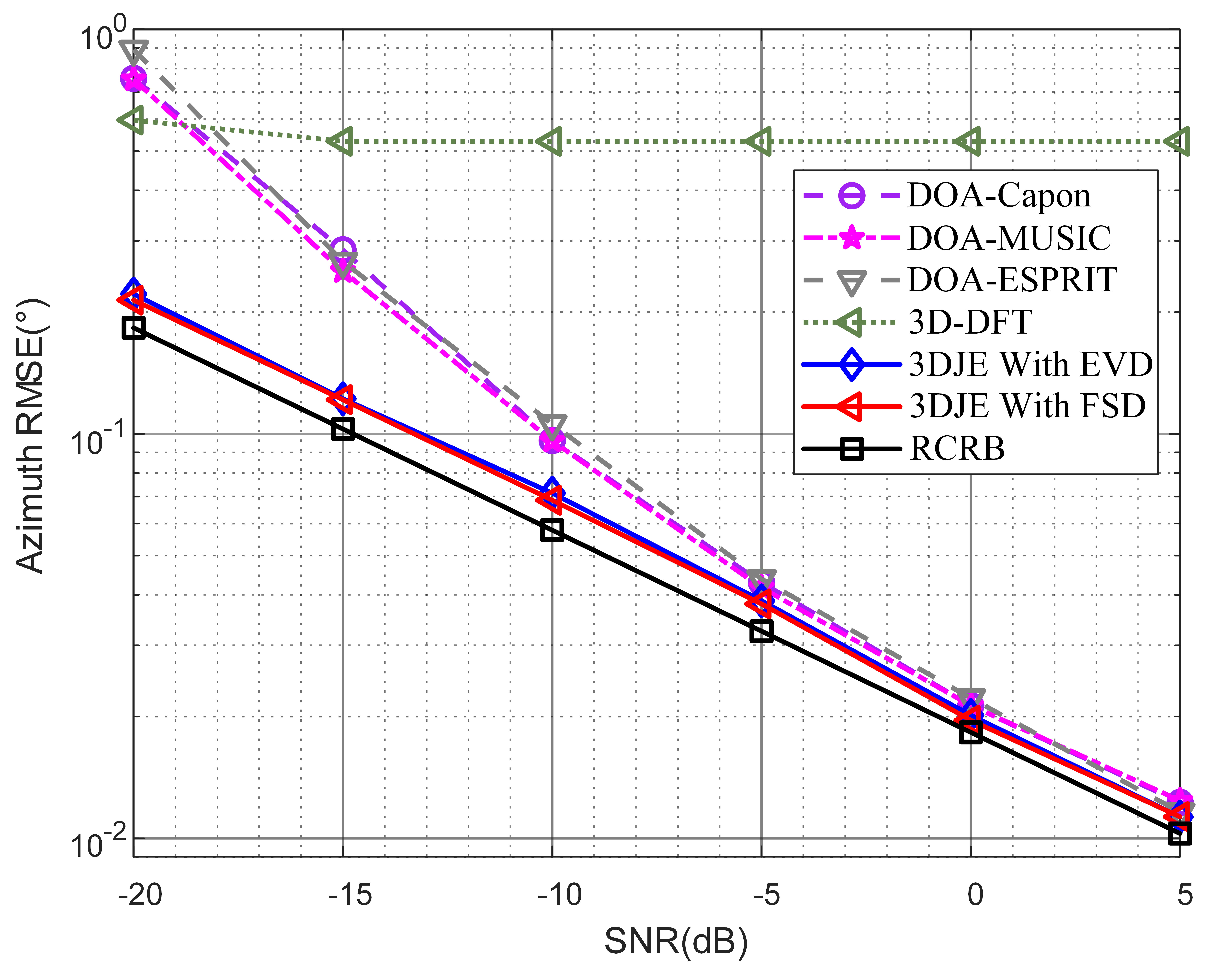
(c) RMSE of azimuth estimation vs SNR.

Figure 3: Single-target estimation RMSE vs SNR for $\Delta f=60\ {\rm{}}\rm kHz$.

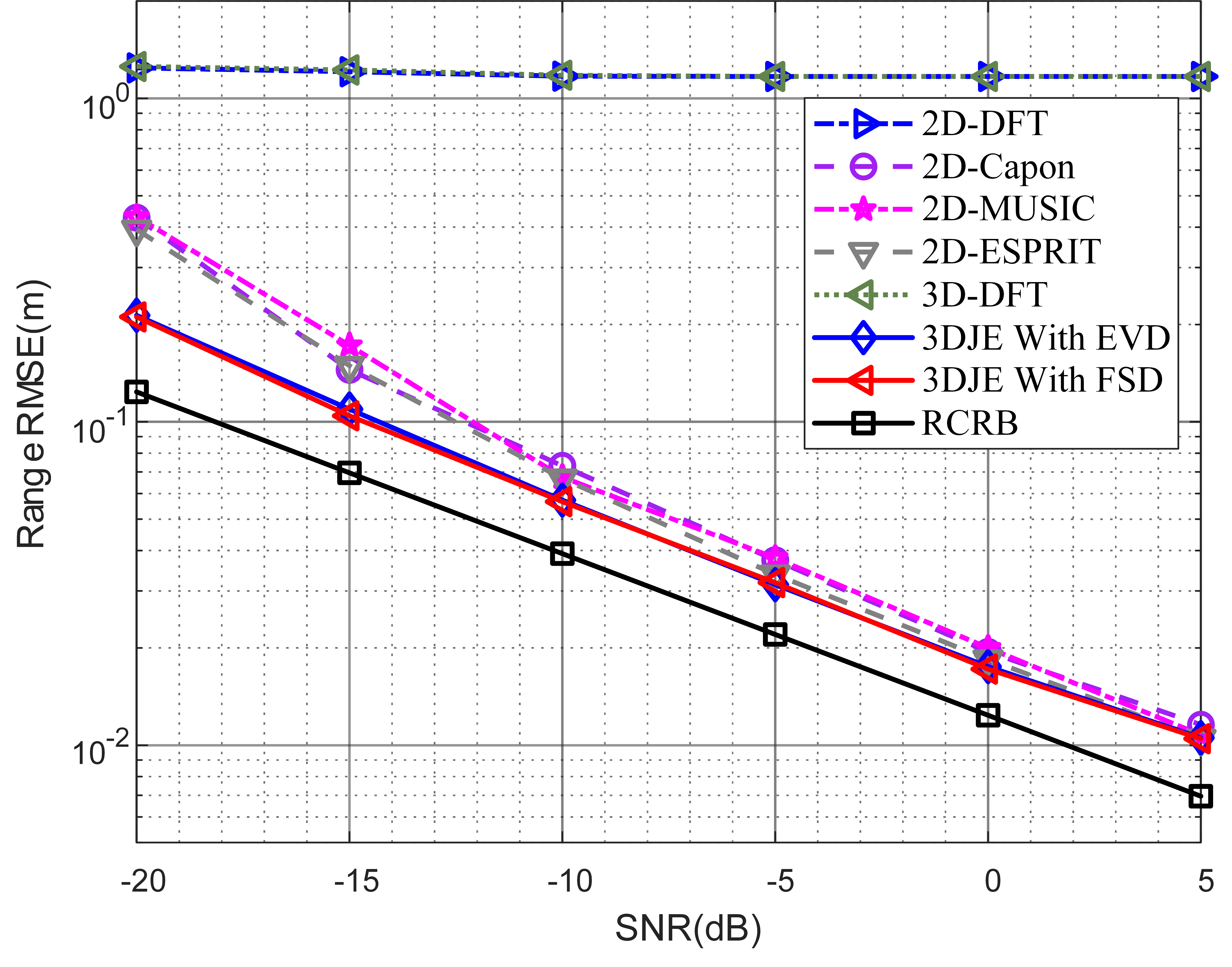
(a) RMSE of range estimation vs SNR.

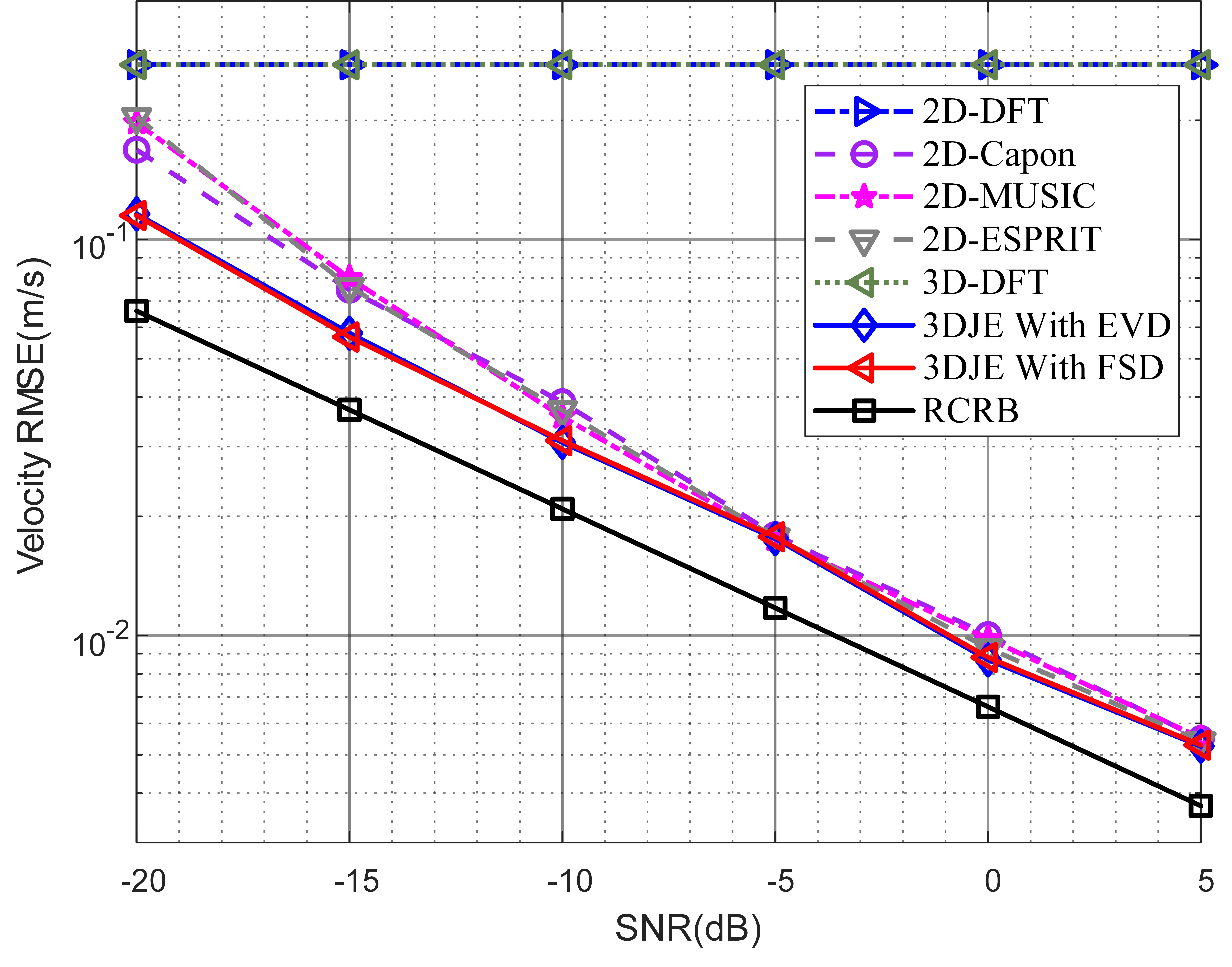
(b) RMSE of velocity estimation vs SNR.

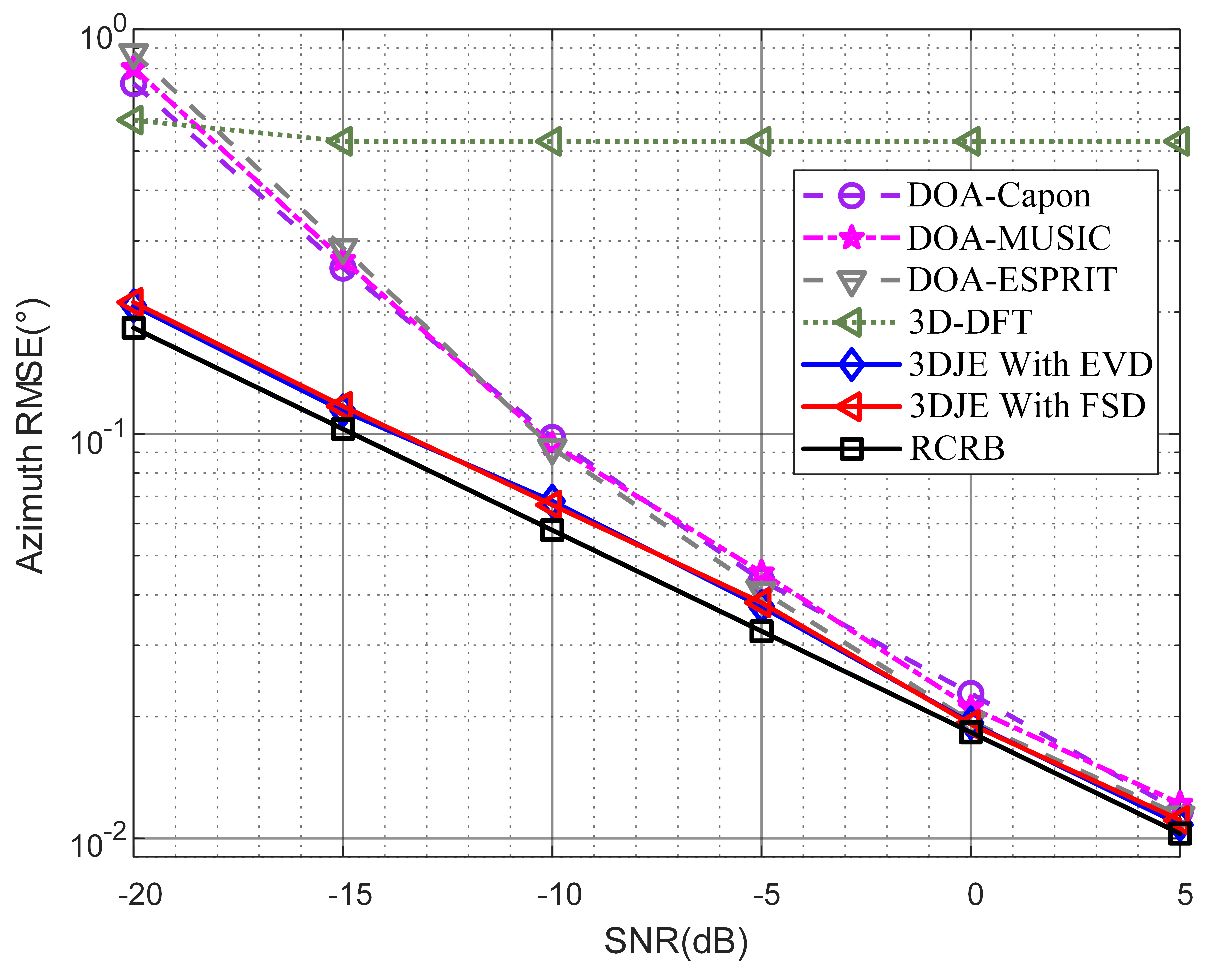
(c) RMSE of azimuth estimation vs SNR.

Figure 4: Single-target estimation RMSE vs SNR for $\Delta f=120\ {\rm{}}\rm kHz$.

As illustrated in Fig. 3 for $\Delta f=$ 60 kHz and Fig. 4 for $\Delta f=$ 120 kHz, respectively. The 3DJE with FSD and 3DJE with EVD denote signal subspace estimation obtained by FSD and EVD, respectively. The 2D-DFT, 2D-MUSIC, 2D-ESPRIT, 2D-Capon and 3D-DFT denote the aforementioned estimation methods which are detailed in [12], [31], [32] and [37]. The DOA-Capon, DOA-MUSIC, and DOA-ESPRIT in legend denote Capon [34], MUSIC [35], and ESPRIT [36] methods for azimuth estimation, respectively. Numerical results show that the proposed 3DJE algorithm with FSD achieves almost the same RMSE performance as the 3DJE with EVD.

In Fig. 3(a) and Fig. 4(a), the RMSE of range estimation with different SNRs is illustrated. The proposed 3DJE algorithm achieves better estimation performance than other algorithms, especially when the SNR is low. Specifically, at a RMSE level of 10^-1, for both $\Delta f=$ 60 kHz and $\Delta f=$ 120 kHz, the proposed algorithm achieves a SNR gain of 2.5 dB compared to the 2D-MUSIC method. Besides, for $\Delta f=$ 120 kHz, the proposed algorithm suffers from about 3.5 dB SNR degradation compared to the RCRB. It is noted that the RMSE of the traditional DFT-based methods (i.e., 2D-DFT and 3D-DFT methods) does not change with the increase of SNR, the reason is that the DFT-based methods can not achieve super-resolution estimation of range, velocity and azimuth, and the range resolution is determined by the bandwidth, that is, $\Delta R={c\mathord{\left/{\vphantom{c{2N\Delta f}}}\right.\kern-1.2pt}{(2B)}}$. Moreover, the proposed algorithm achieves better range estimation performance for $\Delta f=$ 120 kHz than that for $\Delta f=$ 60 kHz.

In Fig. 3(b) and Fig. 4(b), the RMSE of velocity estimation with different SNRs is presented. Fig. 3(b) and Fig. 4(b) show that the proposed 3DJE algorithm achieves better estimation performance than other algorithms, especially when the SNR is low. Specifically, at a RMSE level of 10^-2, compared to the RCRB, the proposed algorithm suffers from only 0.9 dB and 2.7 dB SNR degradation for $\Delta f=$ 60 kHz and $\Delta f=$ 120 kHz, respectively. Since the velocity resolution of DFT-based methods is limited by the CPI, that is, $\Delta v={c\mathord{\left/{\vphantom{c{2{f_{c}}M\bar{T}}}}\right.\kern-1.2pt}{(2{f_{c}}M\bar{T})}}$, the velocity RMSE of DFT-based methods remain constant. Moreover, the proposed algorithm achieves better velocity estimation performance for $\Delta f=$ 60 kHz than that for $\Delta f=$ 120 kHz.

In Fig. 3(c) and Fig. 4(c), the RMSE of azimuth estimation with different SNRs is demonstrated. Fig. 3(c) and Fig. 4(c) demonstrate that the proposed 3DJE algorithm achieves better estimation performance than other algorithms, especially when the SNR is low. Specifically, at a RMSE level of 10^-1, compared to the DOA-MUSIC method, the proposed algorithm achieves a SNR gain of 3.1 dB and 3.3 dB for $\Delta f=$ 60 kHz and $\Delta f=$ 120 kHz, respectively. Besides, compared to the RCRB, the proposed algorithm suffers from only 1.5 dB and 1.3 dB SNR degradation for $\Delta f=$ 60 kHz and $\Delta f=$ 120 kHz, respectively. For the 3D-DFT method, since the performance of azimuth estimation is limited by the array aperture of receive antennas, the azimuth RMSE does not change when SNR $>$ -15 dB. Moreover, when the subcarrier spacing is $\Delta f=$ 60 kHz, the proposed algorithm achieves almost the same azimuth estimation performance as that for $\Delta f=$ 120 kHz.

V-B Estimation Accuracy for Multiple Targets

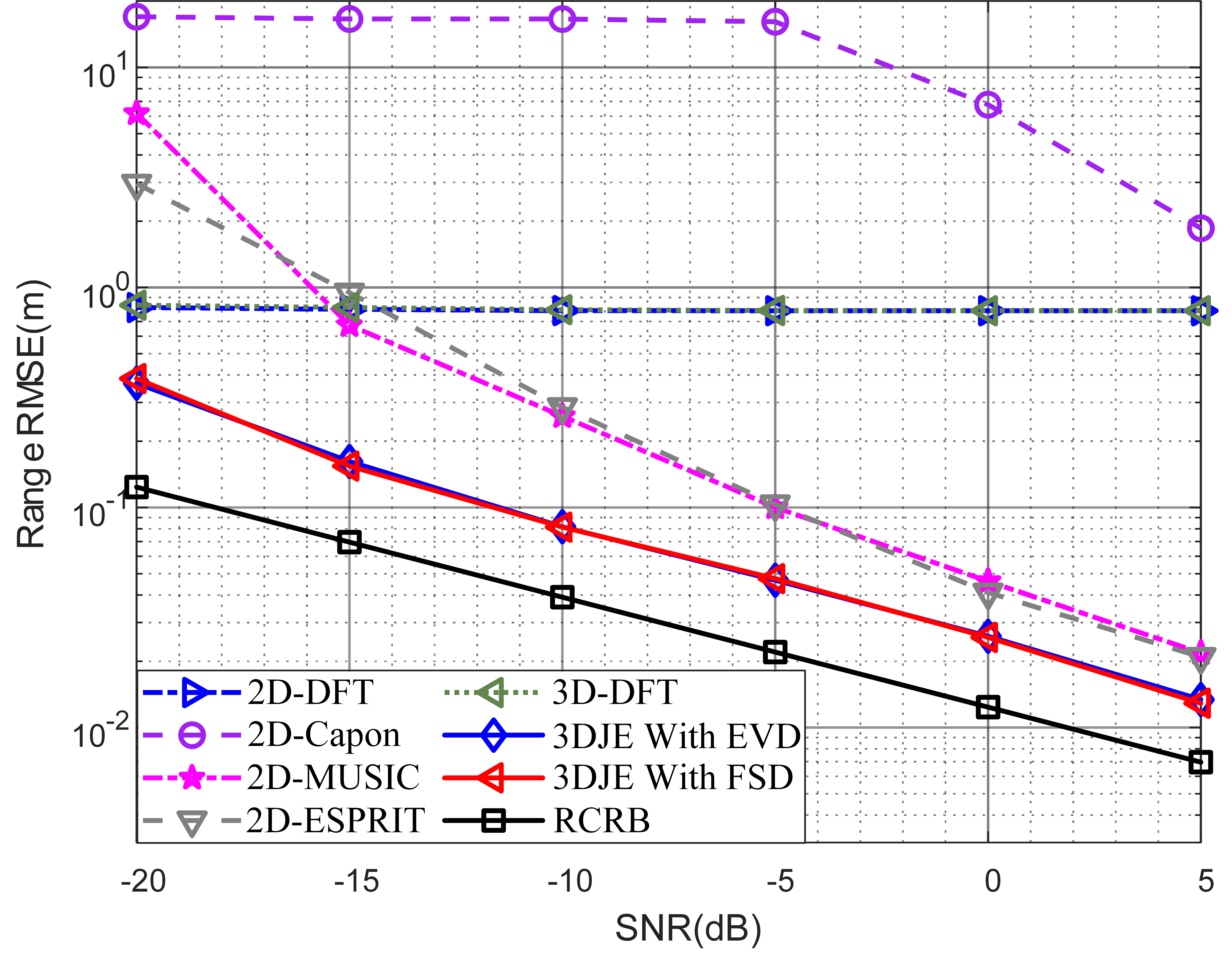
(a) RMSE of range estimation vs SNR.

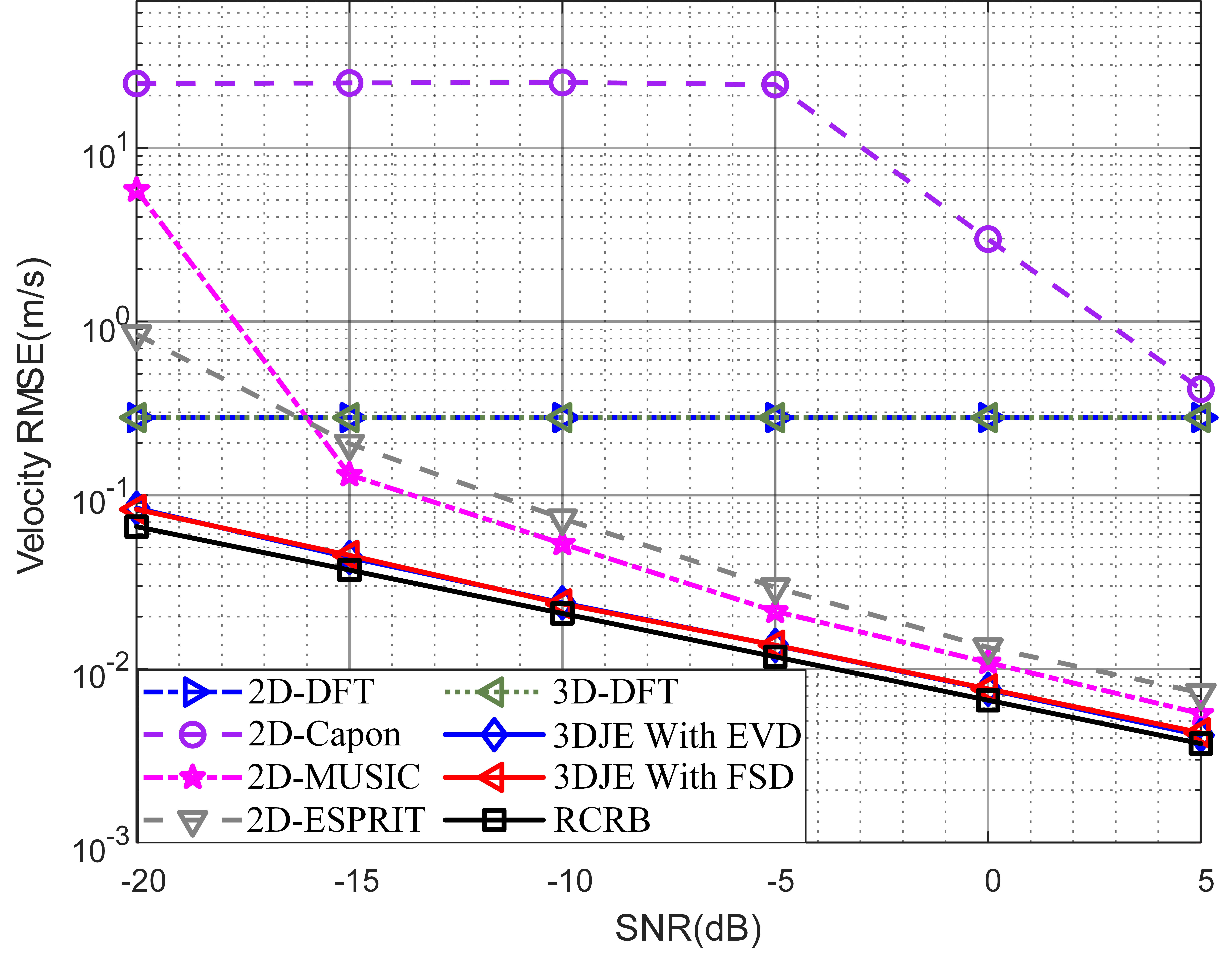
(b) RMSE of velocity estimation vs SNR.

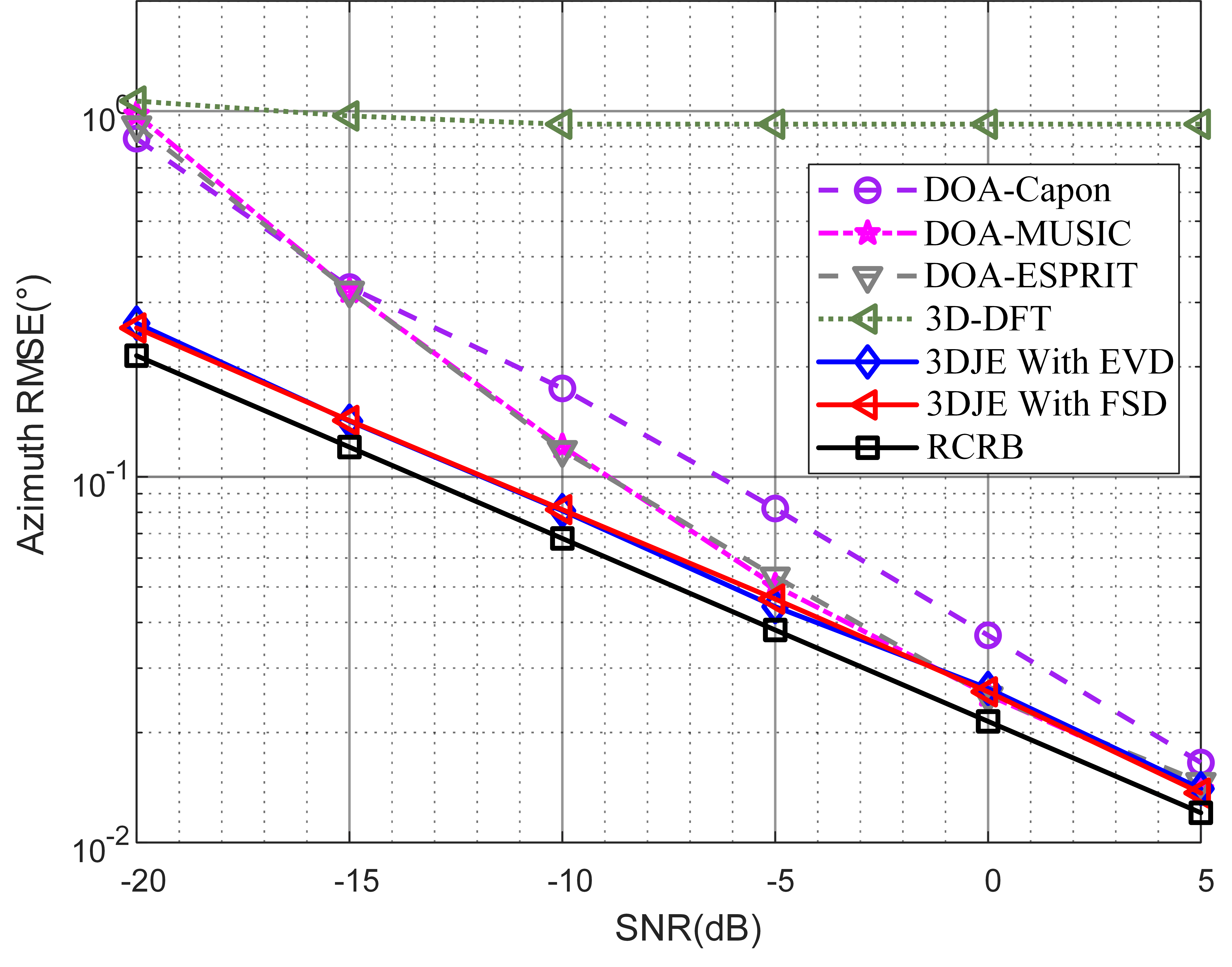
(c) RMSE of azimuth estimation vs SNR.

Figure 5: Multi-target estimation RMSE vs SNR for $\Delta f=60\ {\rm{}}\rm kHz$.

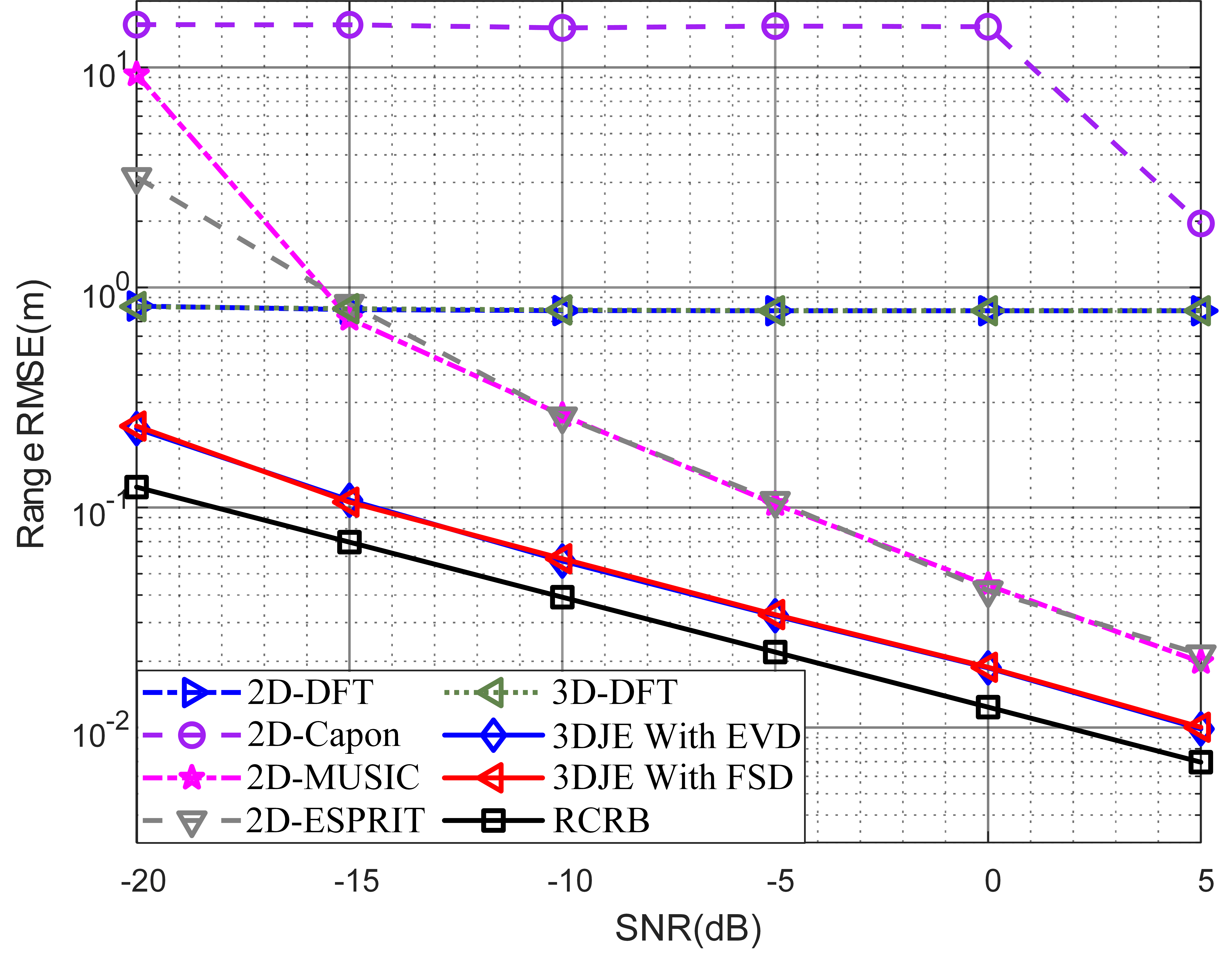
(a) RMSE of range estimation vs SNR.

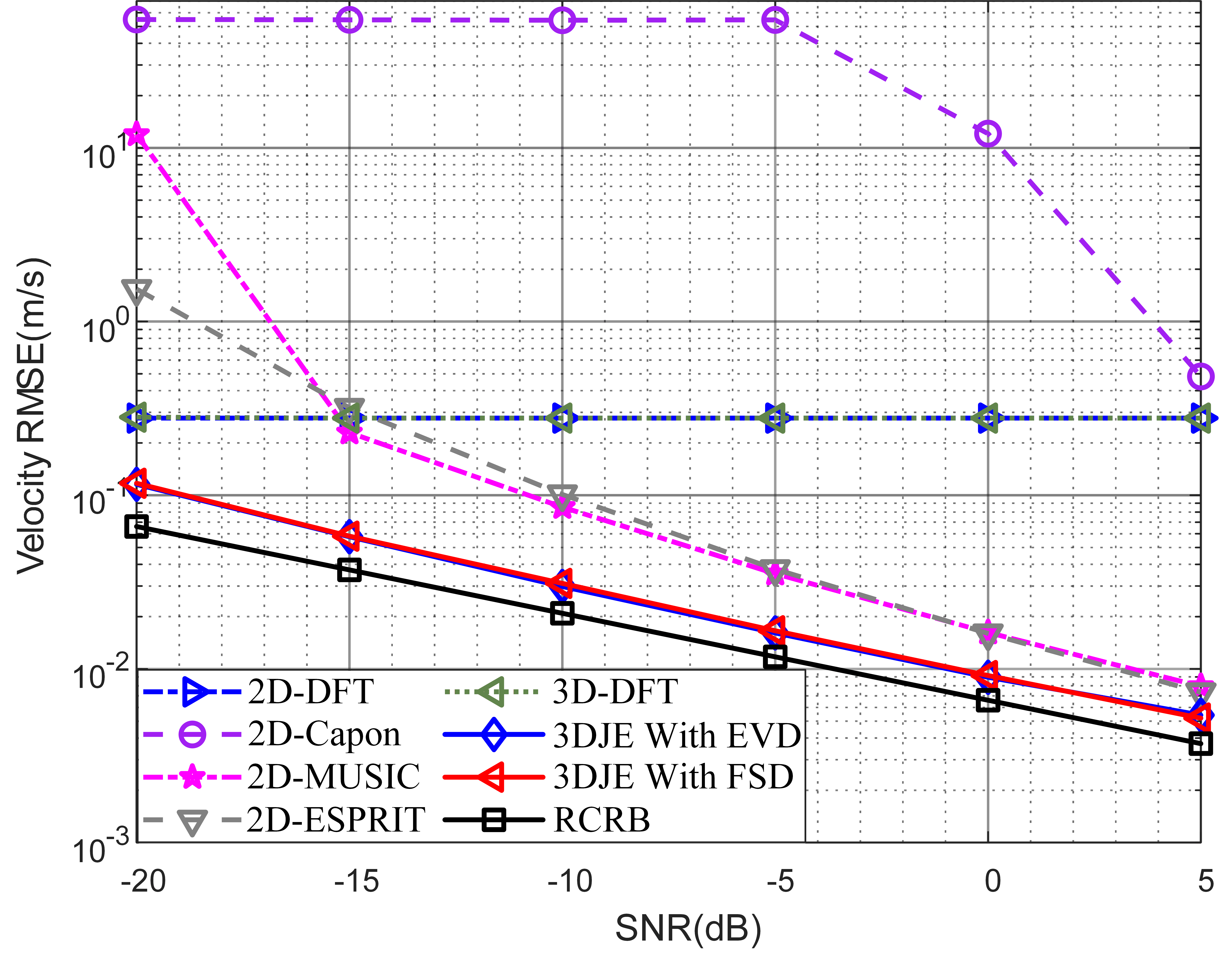
(b) RMSE of velocity estimation vs SNR.

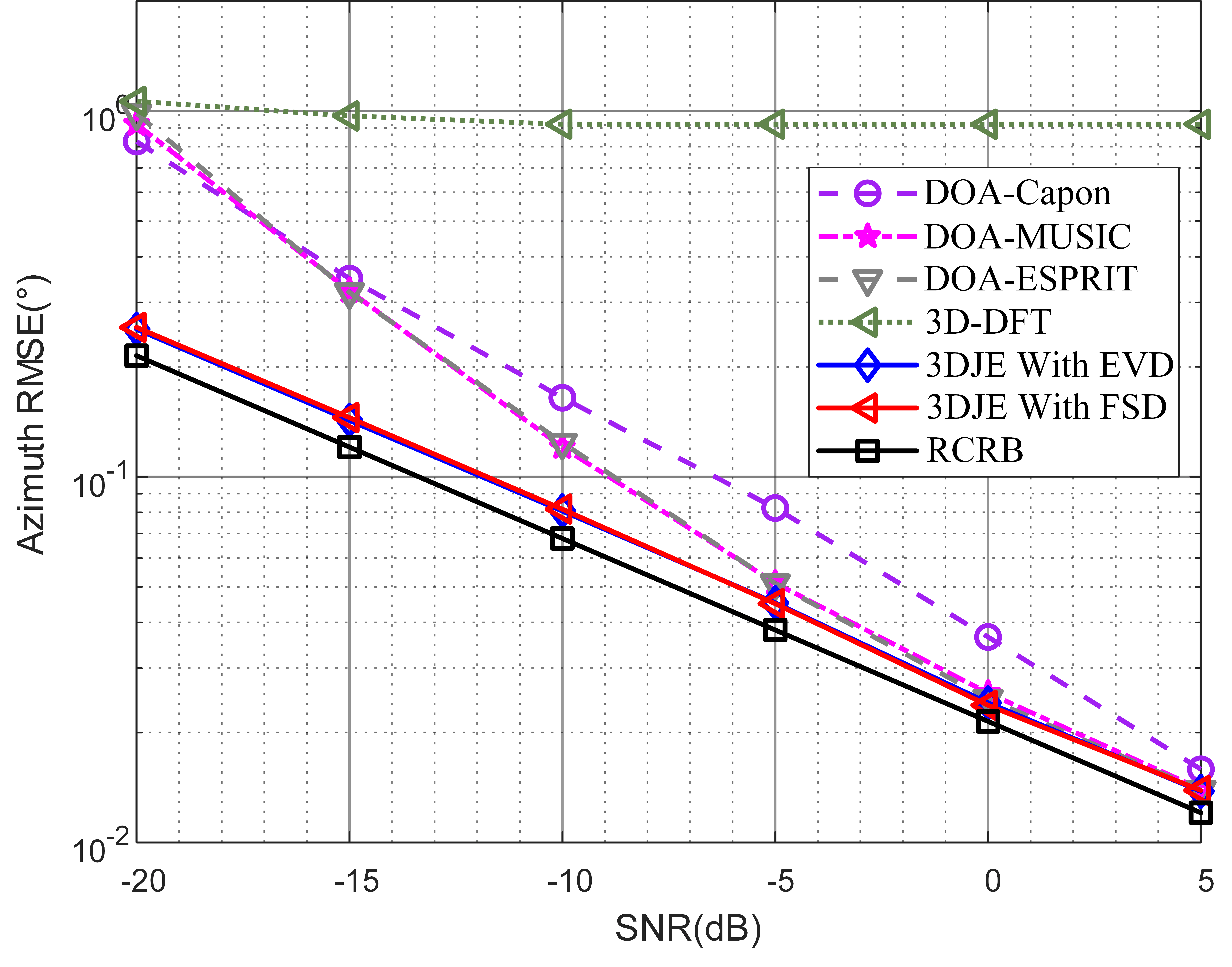
(c) RMSE of azimuth estimation vs SNR.

Figure 6: Multi-target estimation RMSE vs SNR for $\Delta f=120\ {\rm{}}\rm kHz$.

We set the number of targets $K=3$. The range, velocity, and azimuth parameters of the three targets are assumed to be $(35{\rm{m,15m/s,20}}^{\circ})$, $(60{\rm{m,10m/s,-20}}^{\circ})$ and $(80{\rm{m,-10m/s,50}}^{\circ})$, respectively. The SNR varies from -20 dB to 5 dB with an interval of 5 dB. For each SNR, 200 times independent Monte Carlo simulations are performed. The simulation results are shown in Fig. 5 and Fig. 6. Numerical results show that the proposed 3DJE algorithm with FSD achieves almost the same RMSE performance as the 3DJE with EVD.

In Fig. 5(a) and Fig. 6(a), the RMSE of range estimation with different SNRs is illustrated. The proposed algorithm achieves better estimation performance than other algorithms, especially when the SNR is low. Specifically, at a RMSE level of 10^-1, compared to the 2D-MUSIC method, the proposed algorithm achieves a SNR gain of 6.6 dB and 9.6 dB for $\Delta f=$ 60 kHz and $\Delta f=$ 120 kHz, respectively. Besides, for $\Delta f=$ 120 kHz, the proposed algorithm suffers from about 3.6 dB SNR degradation compared to the RCRB. Moreover, the proposed algorithm achieves better range estimation performance for $\Delta f=$ 120 kHz than that for $\Delta f=$ 60 kHz.

In Fig. 5(b) and Fig. 6(b), the RMSE of velocity estimation with different SNRs is presented. Fig. 5(b) and Fig. 6(b) show that the proposed 3DJE algorithm achieves better estimation performance than other algorithms, especially when the SNR is low. Specifically, at a RMSE level of 10^-2, compare to the RCRB, the proposed algorithm suffers from only 1.3 dB and 2.8 dB SNR degradation for $\Delta f=$ 60 kHz and $\Delta f=$ 120 kHz, respectively. Moreover, the proposed algorithm achieves better velocity estimation performance for $\Delta f=$ 60 kHz than that for $\Delta f=$ 120 kHz.

In Fig. 5(c) and Fig. 6(c), the RMSE of azimuth estimation with different SNRs is demonstrated. Fig. 5(c) and Fig. 6(c) show that the proposed 3DJE algorithm achieves better estimation performance than other algorithms, especially when the SNR is low. Specifically, at a RMSE level of 10^-1, compared to the 2D-MUSIC method, the proposed algorithm achieves a SNR gain of 3 dB and 2.9 dB for $\Delta f=$ 60 kHz and $\Delta f=$ 120 kHz, respectively. Besides, compared to the RCRB, the proposed algorithm suffers from only 1.5 dB and 1.6 dB SNR degradation for $\Delta f=$ 60 kHz and $\Delta f=$ 120 kHz, respectively. Moreover, when the subcarrier spacing is $\Delta f=$ 60 kHz, the proposed algorithm achieves almost the same azimuth estimation performance as that for $\Delta f=$ 120 kHz.

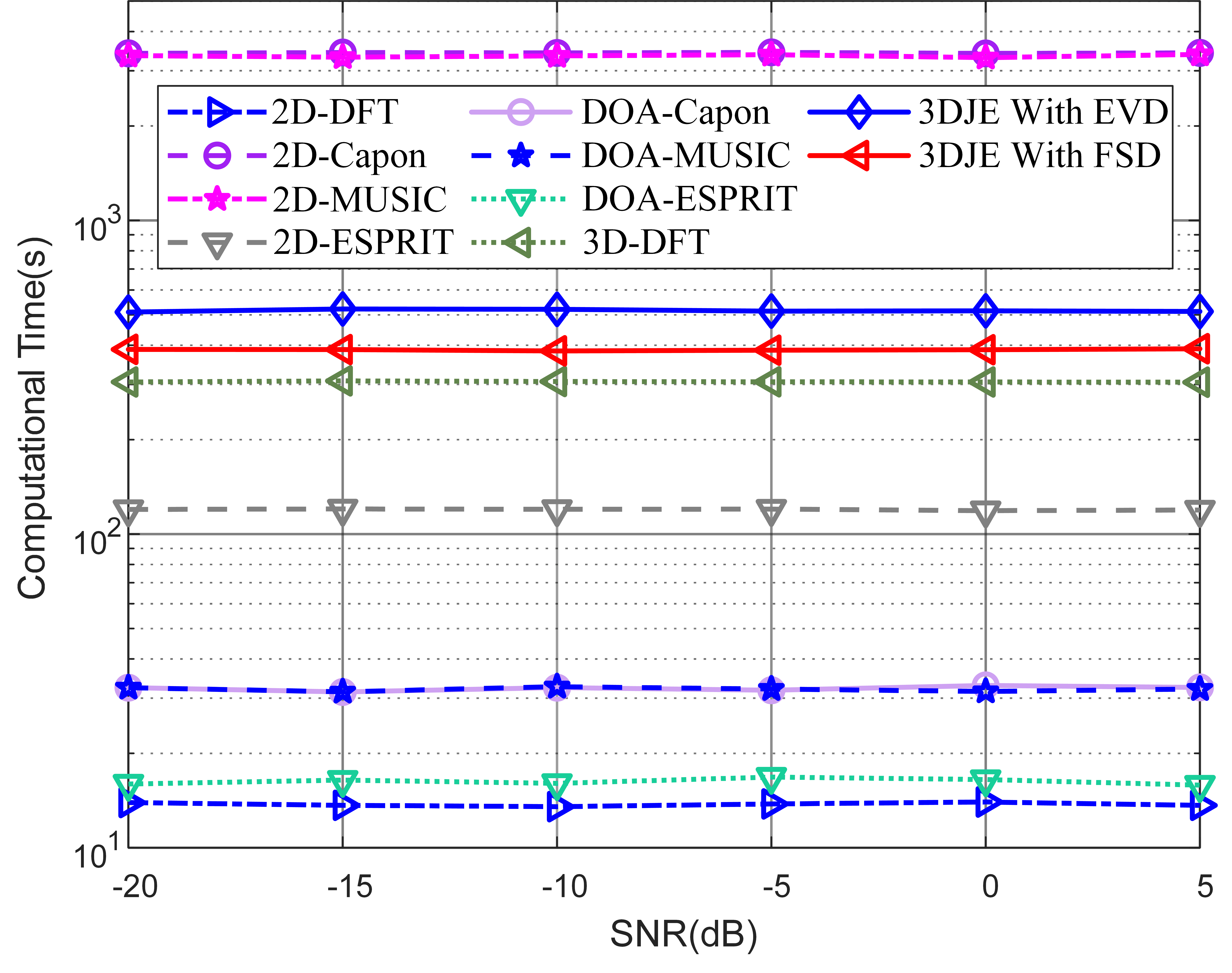
Figure 7: Computational time vs SNR.

Fig. 7 shows the computational time of 200 Monte Carlo simulations with different SNRs. With the increase of SNR, the computational time of the algorithms is almost unchanged. The computational time of the 3DJE with EVD and 3DJE with FSD is about 515.6 s and 387.0 s, respectively. Compared with 3DJE with EVD, 3DJE with FSD reduces approximately 25.0% of computational time and has almost no performance loss. Besides, compared with the 2D-DFT method, the 3D-DFT method requires additional DFT operation in the space domain, which leads to a sharp increase in computational time. In addition, since the 2D-MUSIC and 2D-Capon methods need to search the spectral peaks, they have a longer computational time than the 2D-ESPRIT and 2D-DFT methods. Similarly, the DOA-Capon and DOA-MUSIC methods also have longer computational time than the DOA-ESPRIT method.

VI Conclusion

This paper proposes an auto-paired super-resolution 3DJE algorithm to achieve the joint range-velocity-azimuth estimation for OFDM-based ISAC systems. Simulation results show that compared to the classic 2D-DFT, 2D-MUSIC, 2D-Capon, 2D-ESPRIT and 3D-DFT methods, the proposed algorithm achieves better range and velocity estimation performance. Compared to the classic DOA estimation methods, including DOA-ESPRIT, DOA-MUSIC, DOA-Capon and 3D-DFT, the proposed algorithm achieves better azimuth estimation performance. Besides, the proposed algorithm suffers slightly RMSE performance degradation compared to the RCRB. For future work, we will consider more complicated situations with non-Gaussian white noise, and elevation estimation for OFDM-based ISAC systems.

[Proof of Lemma 1] Let $\mathbf{w}^{\prime}_{p,m}=[{w^{\prime}_{p,m}(0)},{w^{\prime}_{p,m}(1)},\ldots,{w^{\prime}_{p,m}(N\!-\!1)}]^{T}$ and $\mathbf{w}_{p,m}=[w_{p,m}(0),w_{p,m}(1),\ldots,w_{p,m}(N\!-\!1)]^{T}$. Assume that the joint probability density distribution function (PDF) of $\mathbf{w}^{\prime}_{p,m}$ and $\mathbf{w}_{p,m}$ are $f(\mathbf{w}^{\prime})$ and $f(\mathbf{w})$, respectively. $\mathbf{F}$ is defined as the Fourier transform matrix, which can be expressed as

$$\mathbf{F}=\left[{\begin{array}[]{*{20}{c}}1&1&1&\cdots&1\\ 1&\zeta&{{\zeta^{2}}}&\cdots&{{\zeta^{N-1}}}\\ 1&{{\zeta^{2}}}&{{\zeta^{4}}}&\cdots&{{\zeta^{N-2}}}\\ \vdots&\vdots&\vdots&\ddots&\vdots\\ 1&{{\zeta^{N-1}}}&{{\zeta^{N-2}}}&\cdots&\zeta\end{array}}\right],$$ (75)

where $\zeta={{e^{-j{{2\pi}\mathord{\left/{\vphantom{{2\pi}N}}\right.\kern-1.2pt}N}}}}$.

Since ${w^{\prime}_{p,m}}({k})$ is independent and ${w^{\prime}_{p,m}}({k})\sim{\cal C}{\cal N}(0,{\sigma^{2}})$, it is obvious that $\mathbf{w}^{\prime}_{p,m}\sim{\cal C}{\cal N}(\mathbf{0},{\sigma^{2}}\mathbf{I})$. The joint PDF $f(\mathbf{w}^{\prime})$ can be expressed as

$$f({\mathbf{w^{\prime}}})=\frac{1}{{{{(\pi{\sigma^{2}})}^{N}}}}\exp\left\{-\displaystyle\frac{{\left\|{{\mathbf{w^{\prime}}}}\right\|_{2}^{2}}}{{{\sigma^{2}}}}\right\}.$$ (76)

Since $\mathbf{w}_{p,m}=\mathbf{F}\mathbf{w}^{\prime}_{p,m}$, we have $\mathbf{w}_{p,m}\sim{\cal C}{\cal N}(\mathbf{0},{\sigma^{2}}\mathbf{F}\mathbf{F}^{H})$, and the joint PDF $f_{w}(\mathbf{w})$ can be expressed as

$${f}(\mathbf{w})=\frac{1}{{{\pi^{N}}\det({\sigma^{2}}\mathbf{F}{\mathbf{F}^{H}})}}\exp\left\{-\frac{{{\mathbf{w}^{H}}(\mathbf{F}{\mathbf{F}^{H})^{-\!1}}\mathbf{w}}}{{{\sigma^{2}}}}\right\}.$$ (77)

Moreover, since the $\mathbf{F}\mathbf{F}^{H}=N\mathbf{I}$, (77) can be further written as

$${f}(\mathbf{w})=\frac{1}{{{{(\pi N{\sigma^{2}})}^{N}}}}\exp\left\{-\frac{{{{\left\|\mathbf{w}\right\|}_{2}^{2}}}}{{N{\sigma^{2}}}}\right\}.$$ (78)

The PDF in (78) shows that the random variable ${w_{p,m}}({n})$ obeys a complex Gaussian distribution, denoted by ${w_{p,m}}({n})\sim{\cal C}{\cal N}(0,N{\sigma^{2}})$. In addition, the random variables ${w_{p,m}}({n})$ with different frequencies are independent.

Suppose that the modulation order of PSK is $M_{{p}}$, the PSK modulation symbol $s_{m}(n)$ can be expressed as $s_{m}(n)={e^{j\frac{{2\pi q}}{{{M_{p}}}}}}=\cos(\frac{{2\pi q}}{{{M_{p}}}})+j\sin(\frac{{2\pi q}}{{{M_{p}}}})=s_{re}+js_{im}=s$, where $q=0,1,\ldots,M_{{p}}\!-\!1$. It is obvious that $\sum\limits_{q=0}^{{M_{p}\!-\!1}}{P({s_{re}}=\cos\frac{{2\pi q}}{{{M_{p}}}},{s_{{im}}}=\sin\frac{{2\pi q}}{{{M_{p}}}})}=1$.

For convenience, let ${w_{p,m}}(n)=w_{re}+jw_{im}=w$ and ${v_{p,m}}(n)=v_{re}+jv_{im}=v$, since $v=w/s$, we have

$$\begin{array}[]{ll}v&=\displaystyle\frac{w}{s}=\displaystyle\frac{{{w_{re}}+j{w_{im}}}}{{{s_{re}}+j{s_{im}}}}\vspace{0.05cm}\\ &=({w_{re}}{s_{re}}+{w_{im}}{s_{im}})+j({w_{im}}{s_{re}}-{w_{re}}{s_{im}})\\ &={v_{re}}+j{v_{im}}.\end{array}$$ (79)

The PDF of $v_{re}$ can be expressed as

$$\begin{array}[]{ll}f({v_{re}})=\sum\limits_{q=0}^{{M_{p}\!-\!1}}{P({s_{re}}=\cos\frac{{2\pi q}}{{{M_{p}}}},{s_{im}}=\sin\frac{{2\pi q}}{{{M_{p}}}})}\\ \cdot\displaystyle\frac{1}{{\sqrt{\pi(s_{re}^{2}+s_{im}^{2})N{\sigma^{2}}{\text{ }}}}}\exp\left\{{-\frac{{v_{re}^{2}}}{{(s_{re}^{2}+s_{im}^{2})N{\sigma^{2}}{\text{ }}}}}\right\}\\ \ \ \ \ \ \ \ =\displaystyle\frac{1}{\sqrt{\pi N{\sigma^{2}}}}\exp\left\{-\frac{v_{re}^{2}}{N{\sigma^{2}}}\right\}.\end{array}$$ (80)

Similarly, we can obtain that ${v_{im}}\sim{\cal N}(0,N{\sigma^{2}}/2)$. In addition, since ${\rm\mathbb{E}}\{{v_{re}}{v_{im}}\}=0$, $v_{re}$ and $v_{im}$ are mutually independent. Therefore, ${v_{p,m}}(n)=v_{re}+jv_{im}$ obeys a complex Gaussian distribution, denoted by ${v_{p,m}}(n)\sim{\cal C}{\cal N}(0,N{\sigma^{2}})$.

References

- [1] Z. Xiao and Y. Zeng, “Waveform Design and Performance Analysis for Full-Duplex Integrated Sensing and Communication,” IEEE J. Sel. Areas Commun., vol. 40, no. 6, pp. 1823-1837, June 2022.
- [2] J. A. Zhang et al., “An Overview of Signal Processing Techniques for Joint Communication and Radar Sensing,” IEEE J. Sel. Top. Signal Process., vol. 15, no. 6, pp. 1295-1315, Nov. 2021.
- [3] M. F. Keskin, V. Koivunen and H. Wymeersch, “Limited Feedforward Waveform Design for OFDM Dual-Functional Radar-Communications,” IEEE Trans. Signal Process., vol. 69, pp. 2955-2970, 2021.
- [4] Z. Wei et al., “Integrated Sensing and Communication Signals Toward 5G-A and 6G: A Survey,” IEEE Internet Things J., vol. 10, no. 13, pp. 11068-11092, 1 July1, 2023.
- [5] X. Cheng, D. Duan, S. Gao and L. Yang, “Integrated Sensing and Communications (ISAC) for Vehicular Communication Networks (VCN),” IEEE Internet Things J., vol. 9, no. 23, pp. 23441-23451, 1 Dec.1, 2022.
- [6] Y. Huang, S. Hu and G. Wu, “A TDMA approach for OFDM-based multiuser RadCom systems,” China Commun., vol. 20, no. 5, pp. 93-103, May 2023.
- [7] Q. Huang, H. Chen and Q. Zhang, “Joint Design of Sensing and Communication Systems for Smart Homes,” IEEE Netw., vol. 34, no. 6, pp. 191-197, November/December 2020.
- [8] D. Ma, N. Shlezinger, T. Huang, Y. Liu and Y. C. Eldar, “Joint Radar-Communication Strategies for Autonomous Vehicles: Combining Two Key Automotive Technologies,” IEEE Signal Process. Mag., vol. 37, no. 4, pp. 85-97, July 2020.
- [9] K. Meng, Q. Wu, S. Ma, W. Chen, K. Wang and J. Li, “Throughput Maximization for UAV-Enabled Integrated Periodic Sensing and Communication,” IEEE Trans. Wireless Commun., vol. 22, no. 1, pp. 671-687, Jan. 2023.
- [10] M. G. Amin, Y. D. Zhang, F. Ahmad and K. C. D. Ho, “Radar Signal Processing for Elderly Fall Detection: The future for in-home monitoring,” IEEE Signal Process. Mag., vol. 33, no. 2, pp. 71-80, March 2016.
- [11] A. Liu et al., “A Survey on Fundamental Limits of Integrated Sensing and Communication,” IEEE Commun. Surveys Tuts., vol. 24, no. 2, pp. 994-1034, Secondquarter 2022.
- [12] C. Sturm and W. Wiesbeck, “Waveform Design and Signal Processing Aspects for Fusion of Wireless Communications and Radar Sensing, ” Proc. IEEE, vol. 99, no. 7, pp. 1236-1259, July 2011.
- [13] W. Zhou, R. Zhang, G. Chen and W. Wu, “Integrated Sensing and Communication Waveform Design: A Survey,” IEEE Open J. Commun. Soc., vol. 3, pp. 1930-1949, 2022.
- [14] R. Xie, K. Luo and T. Jiang, “Waveform Design for LFM-MPSK-Based Integrated Radar and Communication Toward IoT Applications,” IEEE Internet Things J., vol. 9, no. 7, pp. 5128-5141, 1 April1, 2022.
- [15] Y. Huang, S. Hu, S. Ma, Z. Liu and M. Xiao, “Designing Low-PAPR Waveform for OFDM-Based RadCom Systems,” IEEE Trans. Wireless Commun., vol. 21, no. 9, pp. 6979-6993, Sept. 2022.
- [16] Y. Wu, C. Han, and Z. Chen, “DFT-spread orthogonal time frequency space system with superimposed pilots for terahertz integrated sensing and communication,” IEEE Trans. Wireless Commun., early access, Mar. 6, 2023, doi: 10.1109/TWC.2023.3250267.
- [17] Q. Zhang, H. Sun, X. Gao, X. Wang and Z. Feng, “Time-Division ISAC Enabled Connected Automated Vehicles Cooperation Algorithm Design and Performance Evaluation,” IEEE J. Sel. Areas Commun., vol. 40, no. 7, pp. 2206-2218, July 2022.
- [18] C. Shi, F. Wang, S. Salous and J. Zhou, “Joint Subcarrier Assignment and Power Allocation Strategy for Integrated Radar and Communications System Based on Power Minimization,” IEEE Sensors J., vol. 19, no. 23, pp. 11167-11179, 1 Dec.1, 2019.
- [19] T. Huang, N. Shlezinger, X. Xu, Y. Liu and Y. C. Eldar, “MAJoRCom: A Dual-Function Radar Communication System Using Index Modulation,” IEEE Trans. Signal Process., vol. 68, pp. 3423-3438, 2020.
- [20] Y. Zhou, H. Zhou, F. Zhou, Y. Wu and V. C. M. Leung, “Resource Allocation for a Wireless Powered Integrated Radar and Communication System,” IEEE Wireless Commun. Lett., vol. 8, no. 1, pp. 253-256, Feb. 2019.
- [21] C. Sturm, T. Zwick and W. Wiesbeck, “An OFDM System Concept for Joint Radar and Communications Operations,” in Proc. IEEE 69th Veh. Technol. Conf. (VTC), Apr. 2009, pp. 1-5.
- [22] O. Muta, K. Takata, K. Noguchi, T. Murakami and S. Otsuki, “Device-Free WLAN Based Indoor Localization Scheme With Spatially Concatenated CSI and Distributed Antennas,” IEEE Trans. Veh. Technol., vol. 72, no. 1, pp. 852-865, Jan. 2023.
- [23] C. R. Berger, B. Demissie, J. Heckenbach, P. Willett and S. Zhou, “Signal Processing for Passive Radar Using OFDM Waveforms,” IEEE J. Sel. Top. Signal Process., vol. 4, no. 1, pp. 226-238, Feb. 2010.
- [24] J. E. Palmer, H. A. Harms, S. J. Searle and L. Davis, “DVB-T Passive Radar Signal Processing,” IEEE Trans. Signal Process., vol. 61, no. 8, pp. 2116-2126, April15, 2013.
- [25] E. Dahlman, S. Parkvall, and J. Sköld, 5G NR: The Next Generation Wireless Access Technology. New York, NY, USA: Academic, 2018.
- [26] F. Zhang, Z. Zhang, W. Yu and T. -K. Truong, “Joint Range and Velocity Estimation With Intrapulse and Intersubcarrier Doppler Effects for OFDM-Based RadCom Systems,” IEEE Trans. Signal Process., vol. 68, pp. 662-675, 2020.
- [27] T. Zhang, X. -G. Xia and L. Kong, “IRCI Free Range Reconstruction for SAR Imaging With Arbitrary Length OFDM Pulse,” IEEE Trans. Signal Process., vol. 62, no. 18, pp. 4748-4759, Sept.15, 2014.
- [28] X. Wan, J. Yi, Z. Zhao and H. Ke, “Experimental Research for CMMB-Based Passive Radar Under a Multipath Environment,” IEEE Trans. Aerosp. Electron. Syst., vol. 50, no. 1, pp. 70-85, January 2014.
- [29] D. Schindler, B. Schweizer, C. Knill, J. Hasch and C. Waldschmidt, “Synthetization of Virtual Transmit Antennas for MIMO OFDM Radar by Space-Time Coding,” IEEE Trans. Aerosp. Electron. Syst., vol. 57, no. 3, pp. 1964-1971, June 2021.
- [30] R. Xie, D. Hu, K. Luo and T. Jiang, “Performance Analysis of Joint Range-Velocity Estimator With 2D-MUSIC in OFDM Radar,” IEEE Trans. Signal Process., vol. 69, pp. 4787-4800, 2021.
- [31] C. R. Berger, B. Demissie, J. Heckenbach, P. Willett and S. Zhou, “Signal Processing for Passive Radar Using OFDM Waveforms,” IEEE J. Sel. Top. Signal Process., vol. 4, no. 1, pp. 226-238, Feb. 2010.
- [32] Y. Liu, G. Liao, Y. Chen, J. Xu and Y. Yin, “Super-Resolution Range and Velocity Estimations With OFDM Integrated Radar and Communications Waveform,” IEEE Trans. Veh. Technol., vol. 69, no. 10, pp. 11659-11672, Oct. 2020.
- [33] L. Zheng and X. Wang, “Super-Resolution Delay-Doppler Estimation for OFDM Passive Radar,” IEEE Trans. Signal Process., vol. 65, no. 9, pp. 2197-2210, 1 May1, 2017.
- [34] J. Capon, “High-resolution frequency-wavenumber spectrum analysis,” Proc. IEEE, vol. 57, no. 8, pp. 1408-1418, Aug. 1969.
- [35] R. Schmidt, “Multiple emitter location and signal parameter estimation,” IEEE Trans. Antennas Propag., vol. 34, no. 3, pp. 276-280, March 1986.
- [36] R. Roy and T. Kailath, “ESPRIT-estimation of signal parameters via rotational invariance techniques,” IEEE Trans. Acoust., Speech, Signal Process., vol. 37, no. 7, pp. 984-995, July 1989.
- [37] Y. L. Sit, B. Nuss and T. Zwick, “On Mutual Interference Cancellation in a MIMO OFDM Multiuser Radar-Communication Network,” IEEE Trans. Veh. Technol., vol. 67, no. 4, pp. 3339-3348, April 2018.
- [38] J. A. Zhang et al., “Enabling Joint Communication and Radar Sensing in Mobile Networks—A Survey,” IEEE Commun. Surv. Tut., vol. 24, no. 1, pp. 306-345, Firstquarter 2022.
- [39] M. Wax and T. Kailath, “Detection of signals by information theoretic criteria,” IEEE Trans. Acoust., Speech, Signal Process., vol. 33, no. 2, pp. 387-392, April 1985.
- [40] M. Wax and I. Ziskind, “Detection of the number of coherent signals by the MDL principle,” IEEE Trans. Acoust., Speech, Signal Process., vol. 37, no. 8, pp. 1190-1196, Aug. 1989.
- [41] P. Stoica and A. Nehorai, “MUSIC, maximum likelihood, and Cramer-Rao bound,” IEEE Trans. Acoust., Speech, Signal Process., vol. 37, no. 5, pp. 720-741, May 1989.
- [42] Guanghan Xu and T. Kailath, “Fast subspace decomposition,” IEEE Trans. Signal Process., vol. 42, no. 3, pp. 539-551, March 1994.