Partially factorized variational inference for high-dimensional mixed models

Abstract

While generalized linear mixed models (GLMMs) are a fundamental tool in applied statistics, many specifications — such as those involving categorical factors with many levels or interaction terms — can be computationally challenging to estimate due to the need to compute or approximate high-dimensional integrals. Variational inference (VI) methods are a popular way to perform such computations, especially in the Bayesian context. However, naive VI methods can provide unreliable uncertainty quantification. We show that this is indeed the case in the GLMM context, proving that standard VI (i.e. mean-field) dramatically underestimates posterior uncertainty in high-dimensions. We then show how appropriately relaxing the mean-field assumption leads to VI methods whose uncertainty quantification does not deteriorate in high-dimensions, and whose total computational cost scales linearly with the number of parameters and observations. Our theoretical and numerical results focus on GLMMs with Gaussian or binomial likelihoods, and rely on connections to random graph theory to obtain sharp high-dimensional asymptotic analysis. We also provide generic results, which are of independent interest, relating the accuracy of variational inference to the convergence rate of the corresponding coordinate ascent variational inference (CAVI) algorithm for Gaussian targets. Our proposed partially-factorized VI (PF-VI) methodology for GLMMs is implemented in the R package vglmer. Numerical results with simulated and real data examples illustrate the favourable computation cost versus accuracy trade-off of PF-VI.

Keywords: Bayesian computation; hierarchical models; CAVI; structured VI; data augmentation; random graphs

1 Introduction

Generalized linear mixed models (GLMMs) involve fixed and random effects associated with different sets of covariates (see, e.g., Chapters 2 and 3.4 of wood). They are a foundational and widely used tool across multiple disciplines. In many applications, categorical factors associated with the random effects have a large number of levels (e.g., in the hundreds or thousands), which leads to models with many parameters. When interaction terms are included as random effects, the number of parameters also becomes large very quickly. We refer to the resulting GLMMs as high-dimensional. This setting is common in current social sciences applications; for example, political scientists use GLMMs as part of estimating public opinion at hundreds or thousands of geographic units (e.g., warshaw2012district; broockman2018bias) or rely on models with so-called deep interactions (ghitza). A different application of such models is for recommendation systems where the categorical factors correspond to customer and products (e.g., perry; GaoOwen2017EJS).

In this article, we focus on variational inference (VI) methods for high-dimensional GLMMs. The goal of VI is to approximate a probability distribution $\pi$ — typically the posterior distribution of a Bayesian model — by a more tractable one in a family $\mathcal{Q}$ of approximating distributions (bishop). The arguably most popular VI methodology approximates $\pi$ with the distribution $q^{*}\in\mathcal{Q}$ that minimizes the Kullback-Leibler divergence to $\pi$, where the family $\mathcal{Q}$ assumes independence across parameters (i.e. mean-field assumption), and $q^{*}$ is computed with the so-called coordinate ascent variational inference algorithm (CAVI) — see, e.g.  blei2017variational. While being computationally convenient, the mean-field assumption can lead to poor approximation quality, especially in terms of underestimation of uncertainty relative to $\pi$. This is indeed the case for high-dimensional GLMMs, as we formally show in Section 6 (see in particular Theorem 2). There, we quantify how the degree of variance underestimation of $q^{*}$ relative to $\pi$ increases with the number of observations $n$ and parameters $p$, for GLMMs with Gaussian and binomial likelihood and under some simplifying assumptions. The results suggests that standard mean-field approximations — which we refer to as fully factorized (FF) — do not provide reliable uncertainty quantification for high-dimensional GLMMs.

Motivated by such results, we consider alternative families of variational approximations that differ in the dependence structure they assume on fixed and random effects. In particular, we introduce a partially factorized (PF) family which leads to a favourable trade-off between computational cost and approximation accuracy. We show that, under assumptions similar to the ones of Theorem 2 (see Theorems 3 and 4), the degree of variance underestimation obtained with the PF family does not deteriorate as $n$ and $p$ increase. The same theorems imply also that the convergence rate of the CAVI algorithm required to compute the PF variational approximation does not deteriorate as $n$ and $p$ increases. Equivalently, the number of CAVI iterations required to approximate $q^{*}$ with a fixed level of accuracy does not increase with $n$ and $p$. In terms of practical implications, since the PF family is designed to make the cost per iteration of the associated CAVI algorithm comparable to the classical FF-CAVI algorithm, the results suggests that the improvement in accuracy comes with a negligible increase in computational cost.

The results are based on an interesting duality between the convergence rate of CAVI and the accuracy of the corresponding $q^{*}$. This connection, which is not specific to GLMMs and can be of independent interest, is obtained for general Gaussian distributions in Section 4 (see in particular Theorem 1). Intuitively, the result implies that when the variational approximation is poor in terms of uncertainty quantification, the corresponding CAVI algorithm is also slow to converge and vice versa.

We illustrate our proposed methodology through numerical simulations and a re-analysis of the deep interaction models from ghitza. Despite dealing with more complex settings than the ones analysed in the theoretical part of this paper, the results of the numerical simulations often show expected behavior and illustrate good computational costs versus approximation accuracy trade-offs when using PF-VI. The agreement with the behaviour predicted by our theory suggests that the theoretical conclusions are perhaps informative of a wider range of settings than strictly the ones on which their assumptions are based.

Our approach shares connections to existing work exploring modified or relaxed versions of the mean-field assumption to improve VI accuracy. Examples include reparameterizations methods (ncp-vi; tan2021rvb), collapsed VI (teh2006collapsed; loaiza2022fast; you2023approximated) and structured VI (hoffman2015structured; fasano2022scalable). We discuss in more detail the similarities and differences in Section 3. An appealing feature of our proposed of PF-VI methodology for GLMMs is that the corresponding CAVI algorithm can be defined in closed form and does not require stochastic optimization, resulting in a total cost of the overall methodology that scales only linearly with $n$ and $p$, while providing provably improved uncertainty quantification.

The article is organized as follows. Section 2 describes the basic notation and the GLMMs we consider. Section 3 introduces the PF family and the corresponding CAVI algorithm in a general setting. The specific case of GLMMs with Gaussian and binomial likelihood, including full computational and implementation details, are postponed to Section 5. Section 4 establishes the connection between the approximation accuracy of $q^{*}$ and the convergence speed of CAVI for general Gaussian distributions, for both fully and partially factorized families. Section 6 provides a theoretical analysis of the performances of VI with different factorization families in the context of high-dimensional GLMMs. Section 7 showcases the methodology and theory on numerical experiments, which can be reproduced using code found at https://github.com/mgoplerud/pfvi_glmm_replication. The Appendix contains proofs and additional theoretical results.

2 Generalized linear mixed models

We consider GLMMs of the form

$$y_{i} \mid\eta_{i}\sim f(y_{i}|\eta_{i}),\quad\eta_{i}=\bm{x}_{i}^{T}\bm{\beta}+\sum_{k=1}^{K}\bm{z}_{i,k}^{T}\bm{\alpha}_{k}, i=1,\dots,n,$$ (1)

$$\bm{\alpha}_{k,g} \sim\mathcal{N}\left(\bm{0},\gamma\bm{\Sigma}_{k}\right),\quad\bm{\alpha}_{k}=(\bm{\alpha}_{k,1}^{T},\cdots,\bm{\alpha}_{k,G_{k}}^{T})^{T}, g=1,\dots,G_{k};k=1,\dots,K.$$

Here $n$ denotes the number of observations, $\eta_{i}\in\mathbb{R}$ are linear predictors, $\bm{\beta}\in\mathbb{R}^{D_{0}}$ are commonly referred to as “fixed effects” (e.g., diggle) and the corresponding covariates $\bm{x}_{i}\in\mathbb{R}^{D_{0}}$ contains an intercept and other variables of interest — such as the respondent’s income in our analyses in Section 7. Throughout, we interpret $d$ dimensional vectors as $d\times 1$ matrices. The model contains $K$ sets of “random effects,” $\bm{\alpha}_{k}$ for $k\in\{1,\cdots,K\}$, corresponding to categorical factors with $G_{k}$ levels each — such as the state in which a survey respondent lives. The associated parameters, $\bm{\alpha}_{k,g}\in\mathbb{R}^{D_{k}}$ for $g=1,\dots,G_{k}$, have corresponding covariates $\bm{w}_{i,k}\in\mathbb{R}^{D_{k}}$ and are assigned a normal prior. A classic “random intercept” model has $D_{k}=1$ and $\bm{w}_{i,k}=1$, while models with $D_{k}>1$ are commonly referred to as ones with “random slopes.” For each factor $k$, an observation $i$ is assigned to exactly one level whose membership is encoded in the “one-hot” vector $\bm{m}_{i,k}=(m_{i,k,1},\dots,m_{i,k,G_{k}})\in\{0,1\}^{G_{k}}$ with $\sum_{g=1}^{G_{k}}m_{i,k,g}=1$. For compactness, we defined the vector $\bm{\alpha}_{k}=(\bm{\alpha}_{k,1}^{T},\dots,\bm{\alpha}_{k,G_{K}}^{T})^{T}\in\mathbb{R}^{G_{k}D_{k}}$ with covariates $\bm{z}_{i,k}=\bm{m}_{i,k}\otimes\bm{w}_{i,k}\in\mathbb{R}^{G_{k}D_{k}}$, where $\otimes$ denotes the Kronecker product, so that $\bm{z}_{i,k}^{T}\bm{\alpha}_{k}=\sum_{g=1}^{G_{k}}m_{i,k,g}\bm{w}_{i,k}^{T}\bm{\alpha}_{k,g}$.

In this article, we focus on two important special cases of model (1), which vary by the choice of likelihood function $f(y_{i}|\eta_{i})$. First, we assume that $f(y_{i}|\eta_{i})$ is Gaussian with an identity link and, following common practice and existing software implementations (e.g., bates2015lmer; wood), we scale the variance of the random effects by the residual variance. This leads to

$$f(\cdot|\eta_{i}) =\mathcal{N}\left(\eta_{i},\sigma^{2}\right)\,,\quad\gamma=\sigma^{2}\,.$$ (2)

Second, we consider a binomial model with a logistic link function where, for computational and theoretical reasons, we use Polya-Gamma data augmentation (polson2013polyagamma) that introduces additional latent variables $\omega_{i}$. This leads to

$$f(\cdot|\eta_{i}) =\mathrm{Binomial}\left(n_{i},\frac{\exp(\eta_{i})}{1+\exp(\eta_{i})}\right)\,,\quad\gamma=1\,,$$ (3)

$$p(y_{i},\omega_{i}\mid\eta_{i}) =\frac{1}{2^{n_{i}}}\exp\left(\left[y_{i}-n_{i}/2\right]\eta_{i}-\omega_{i}\frac{\eta_{i}^{2}}{2}\right)f_{PG}(\omega_{i}|n_{i},0)\,;$$

where $f_{PG}(\omega|b,c)$ indicates a Polya-Gamma variable with parameters $b$ and $c$. Section 8 discusses extensions beyond these settings.

We adopt a Bayesian approach and assign prior distributions to the model parameters. In particular, the fixed effects $\bm{\beta}$ are assigned improper flat priors and the matrices $\bm{\Sigma}_{k}$ are given inverse Wishart distributions, $\mathrm{IW}(a_{k}^{0},\bm{\Phi}_{k}^{0})$, which become simply inverse gamma distributions when $D_{k}=1$. In the Gaussian model, we also assign the improper prior $1/\sigma^{2}$ to the residual variance parameter.

Throughout the article we denote by $\bm{\theta}=(\bm{\theta}_{0},\bm{\theta}_{1},\dots,\bm{\theta}_{K})=(\bm{\beta},\bm{\alpha}_{1},\dots,\bm{\alpha}_{K})$ the vector of all fixed and random effects. We let $\bm{\phi}$ denote the collection of all $\bm{\Sigma}_{k}$ and any additional parameters or latent variables, e.g., the residual variance $\sigma^{2}$ in the Gaussian model or the Polya-Gamma latent variables $(\omega_{i})_{i=1}^{n}$ in the binomial model.

3 Partially factorized VI

We consider variational approximations $q^{*}(\bm{\theta},\bm{\phi})$ of $p(\bm{\theta},\bm{\phi}\mid\bm{y})$ defined as

$$q^{*}=\operatorname*{arg\,max}_{q\in\mathcal{Q}}\mathbb{E}_{q(\bm{\theta},\bm{\phi})}\left[\log p(\bm{\theta},\bm{\phi},\bm{y})-\log q(\bm{\theta},\bm{\phi})\right].$$ (4)

The expectation maximized in (4) is usually referred to as evidence lower bound (ELBO). We note that while in our context $p(\bm{\theta},\bm{\phi}\mid\bm{y})$ represents the joint posterior distribution of unknown parameters for GLMMs defined in Section 2, the notation and formulas of this section apply to arbitrary distributions defined over a set of variables $(\bm{\theta},\bm{\phi})=(\bm{\theta}_{0},\ldots,\bm{\theta}_{K},\bm{\phi})$.

We consider approximations $q^{*}$ arising from different choices for the family of approximating densities $\mathcal{Q}$, which differ in the factorization they assume across the elements of $\bm{\theta}$. First, we define the fully factorized (FF) family as

$$\mathcal{Q}_{FF}=\left\{q\,:\,q(\bm{\theta},\bm{\phi})=\left[\prod_{k=0}^{K}q(\bm{\theta}_{k})\right]q\left(\bm{\phi}\right)\right\},$$ (5)

where the above notation refers to the set of all joint probability distributions over $(\bm{\theta},\bm{\phi})$ that factorize as indicated. Second, we define the unfactorized (UF) family as

$$\mathcal{Q}_{UF}=\left\{q\,:\,q(\bm{\theta},\bm{\phi})=q(\bm{\theta})q(\bm{\phi})\right\}.$$ (6)

Finally, we define the partially factorized (PF) family as

$$\mathcal{Q}_{PF} =\left\{q\,:\,q(\bm{\theta},\bm{\phi})=q\left(\bm{\theta}_{\mathcal{C}}|\bm{\theta}_{\mathcal{U}}\right)\left[\prod_{k\in\mathcal{U}}q(\bm{\theta}_{k})\right]q(\bm{\phi})\right\}\,,$$ (7)

where $\bm{\theta}_{\mathcal{C}}=(\bm{\theta}_{k})_{k\in\mathcal{C}}$, $\bm{\theta}_{\mathcal{U}}=(\bm{\theta}_{k})_{k\in\mathcal{U}}$ and $(\mathcal{C},\mathcal{U})$ is an arbitrary partition of $\{0,\dots,K\}$ in two blocks, i.e. $\mathcal{C}\subseteq\{0,\ldots,K\}$ and $\mathcal{U}=\{0,\ldots,K\}\setminus\mathcal{C}$. Note that when $\mathcal{C}=\emptyset$ we obtain $\mathcal{Q}_{PF}=\mathcal{Q}_{FF}$ while when $\mathcal{C}=\{0,\ldots,K\}$ we obtain $\mathcal{Q}_{PF}=\mathcal{Q}_{UF}$.

3.1 Partially-Factorized CAVI

The solution $q^{*}$ of the optimization problem defined in (4) is usually computed using CAVI, which is a coordinate ascent algorithm that scans through the terms in the factorization defined by $\mathcal{Q}$, maximizing the objective function in (4) with respect to one term while holding the other terms fixed. For example, one iteration of the CAVI algorithm corresponding to $\mathcal{Q}=\mathcal{Q}_{FF}$, which we refer as FF-CAVI, first updates $q(\bm{\phi})$ given $\{q(\bm{\theta}_{k})\}_{k=0,\dots,K}$ and then $q(\bm{\theta}_{k})$ given $q(\bm{\phi})$ and $\{q(\bm{\theta}_{j})\}_{j\neq k}$ for $k=0,\dots,K$. For many classes of models and factorizations, the optimal distributions solving the conditional maximization steps belong to specific parametric families and, as a result, the updating of factors boils down to updating their parameters.

Whereas the CAVI steps for $\mathcal{Q}_{FF}$ are quite standard and can be found in textbooks (e.g., bishop, ch. 10), those for $\mathcal{Q}_{PF}$ are less so. The following proposition characterises the coordinate-wise optimization for each of the densities involved in the factorization. The proof is simple but instructive as it introduces a key intermediate distribution in (11) that our theory focuses on; hence, we include it after the statement of the result.

Proposition 1.

Let $p(\bm{\theta},\bm{\phi}\mid\bm{y})$ be the target density and $\mathcal{Q}_{PF}$ be defined in (7). Then, the coordinate-wise optimizers of the objective function (4) are as follows:

$$q(\bm{\phi}) \leftarrow{1\over c}\exp\left\{\mathbb{E}_{q(\bm{\theta})}[\log p(\bm{\theta},\bm{\phi},\bm{y})]\right\}$$ (8)

$$q(\bm{\theta}_{\mathcal{C}}\mid\bm{\theta}_{\mathcal{U}}) \leftarrow{\exp\left\{\mathbb{E}_{q(\bm{\phi})}[\log p(\bm{\theta},\bm{\phi},\bm{y})]\right\}\over\int\exp\left\{\mathbb{E}_{q(\bm{\phi})}[\log p(\bm{\theta},\bm{\phi},\bm{y})]\right\}\mathrm{d}\bm{\theta}_{\mathcal{C}}}$$ (9)

$$q(\bm{\theta}_{k}) \leftarrow{1\over c}\exp\left\{\mathbb{E}_{q(\bm{\theta}_{\mathcal{U}\backslash k})}\left[\log\int\exp\left\{\mathbb{E}_{q(\bm{\phi})}[\log p(\bm{\theta},\bm{\phi},\bm{y})]\right\}\mathrm{d}\bm{\theta}_{\mathcal{C}}\right]\right\},\quad k\in\mathcal{U},$$ (10)

where $c$ is a different constant of intergration in each case, $q\left(\bm{\theta}\right)=q\left(\bm{\theta}_{\mathcal{C}}|\bm{\theta}_{\mathcal{U}}\right)\left[\prod_{k\in\mathcal{U}}q(\bm{\theta}_{k})\right]$, $q(\bm{\theta}_{\mathcal{U}\backslash k})=\prod_{m\in\mathcal{U},m\neq k}q(\bm{\theta}_{m})$, and where the updates in (10) assume that $q(\bm{\theta}_{\mathcal{C}}|\bm{\theta}_{\mathcal{U}})$ has already been updated according to (9).

Proof.

The update in (8) is obtained by a standard argument for mean field CAVI, see e.g. (bishop, Ch.10). The ones in (9) and (10) are obtained as follows. Let

$$\pi(\bm{\theta})={\exp\left\{\mathbb{E}_{q(\bm{\phi})}[\log p(\bm{\theta},\bm{\phi},\bm{y})]\right\}\over\int\exp\left\{\mathbb{E}_{q(\bm{\phi})}[\log p(\bm{\theta},\bm{\phi},\bm{y})]\right\}\mathrm{d}\bm{\theta}}$$ (11)

be a probability distribution over $\bm{\theta}$. Note that $\pi(\bm{\theta})$ depends on $q(\bm{\phi})$. Then, it holds

$$\mathbb{E}_{q(\bm{\theta},\bm{\phi})}\left[\log p(\bm{\theta},\bm{\phi},\bm{y})-\log q(\bm{\theta},\bm{\phi})\right]=\mathbb{E}_{q(\bm{\theta})}\left[\log\frac{\pi(\bm{\theta}_{\mathcal{C}}|\bm{\theta}_{\mathcal{U}})}{q(\bm{\theta}_{\mathcal{C}}|\bm{\theta}_{\mathcal{U}})}\right]+\mathbb{E}_{q(\bm{\theta}_{\mathcal{U}})}\left[\log\frac{\pi(\bm{\theta}_{\mathcal{U}})}{q(\bm{\theta}_{\mathcal{U}})}\right]+c\,,$$

where $c$ contains terms that do not depend on $q(\bm{\theta})$. Optimizing this over $q(\bm{\theta}_{\mathcal{C}}|\bm{\theta}_{\mathcal{U}})$ we obtain directly that the optimizer is $\pi(\bm{\theta}_{\mathcal{C}}|\bm{\theta}_{\mathcal{U}})$, hence derive (9). Given $q(\bm{\theta}_{\mathcal{C}}|\bm{\theta}_{\mathcal{U}})=\pi(\bm{\theta}_{\mathcal{C}}|\bm{\theta}_{\mathcal{U}})$ and $q(\bm{\theta}_{\mathcal{U}})=\prod_{k\in\mathcal{U}}q(\bm{\theta}_{k})$, we obtain that the $q(\bm{\theta}_{k})$ coordinate-wise updates maximize

$$\mathbb{E}_{q(\bm{\theta}_{\mathcal{U}})}\left[\log\frac{\pi(\bm{\theta}_{\mathcal{U}})}{\prod_{k\in\mathcal{U}}q(\bm{\theta}_{k})}\right]+c,$$ (12)

where $c$ contains terms that do not depend on $q(\bm{\theta}_{\mathcal{U}})$. The expression in (10) follows by the fact that the objective function in (12) coincides with the one of standard mean field CAVI applied to $\pi(\bm{\theta}_{\mathcal{U}})$, and by the definition of $\pi(\bm{\theta})$. ∎

Given Proposition 1, the CAVI algorithm for $\mathcal{Q}_{PF}$, which we refer to as PF-CAVI, is simply obtained by scanning sequentially through the conditional updates in (8)-(10), as detailed in Algorithm 1.

Input: target distribution $p(\bm{\theta},\bm{\phi}\mid\bm{y})$; sets $\mathcal{C}\subseteq\{0,\ldots,K\}$ and $\mathcal{U}=\{0,\ldots,K\}\setminus\mathcal{C}$

Initialize $q_{0}(\bm{\phi})$, $q_{0}\left(\bm{\theta}_{\mathcal{C}}|\bm{\theta}_{\mathcal{U}}\right)$ and $q_{0}(\bm{\theta}_{k})$ for $k\in\mathcal{U}$

for $t=1:T$ do

     Update $q_{t}(\bm{\phi})$ according to (8)

     Update $q_{t}(\bm{\theta}_{\mathcal{C}}|\bm{\theta}_{\mathcal{U}})$ according to (9)

     for $k\in\mathcal{U}$ do

         Update $q_{t}(\bm{\theta}_{k})$ according to (10)

     end for

end for

Output $q_{T}(\bm{\theta})=q_{T}\left(\bm{\theta}_{\mathcal{C}}|\bm{\theta}_{\mathcal{U}}\right)\left[\prod_{k\in\mathcal{U}}q_{T}(\bm{\theta}_{k})\right]q_{T}(\bm{\phi})$

Algorithm 1 PF-CAVI

It is useful to contrast the range of applicability of PF-CAVI relative to the common FF-CAVI. Being basically equivalent, the update of $q(\bm{\phi})$ is computable in closed form in most situations where the one for FF-CAVI is. Similarly, the update of $q(\bm{\theta}_{\mathcal{C}}\mid\bm{\theta}_{\mathcal{U}})$ is at least as easy as the corresponding FF-CAVI one, since in (9) we condition on $\bm{\theta}_{\mathcal{U}}$ rather than integrating it out in the associated computations. The update of $q(\bm{\theta}_{k})$ for $k\in\mathcal{U}$, instead, requires an additional integration (with respect to $\bm{\theta}_{\mathcal{C}}$) relative to FF-CAVI, and it can be considerably harder for PF-CAVI. Section 5 shows how to carry out this step efficiently when using PF-VI for GLMMs — note that for both Gaussian and binomial GLMMs, $\pi(\bm{\theta})$ is a high-dimensional Gaussian distribution (see e.g. Proposition 4). In general, one should expect the computational cost of PF-CAVI to grow with the size of $\mathcal{C}$, Section 5.2 provides more details.

3.2 Comparison with related work on VI factorizations

Previous work has considered variations of the mean-field assumption — as we do above — in order to improve VI accuracy, both in the context of GLMMs as well as for other Bayesian hierarchical models. In this section, we briefly discuss some of this work and its connections to our approach.

In the GLMM context, ncp-vi; tan2021rvb consider reparameterization techniques, i.e. applying mean-field VI to a (linear) transformation of the parameters, while menictas2023streamlined; goplerud2022mavb consider blocking, i.e. grouping together some parameters in the mean-field factorization. Using our notation, the blocking analogue of $\mathcal{Q}_{PF}$ would be the family $\mathcal{Q}_{B}=\left\{q\,:\ q(\bm{\theta},\bm{\phi})=q\left(\bm{\theta}_{\mathcal{C}}\right)\left[\prod_{k\in\mathcal{U}}q(\bm{\theta}_{k})\right]q(\bm{\phi})\right\}$. While helpful in improving VI accuracy, blocking techniques do not achieve the same level of computational-accuracy trade-off as the partial factorization we propose for GLMMs, see e.g. the comparison and tension between factorizations I, II and III discussed in menictas2023streamlined and discussion on future work in Section 8.

A different approach integrates out certain blocks and applies mean-field VI to the resulting marginal distribution, see work on “collapsed” variational inference in the context of variable selection models (you2023approximated) or models with global and local variables (teh2006collapsed; loaiza2022fast). A closely related approach, which is more directly related to ours, considers partial factorizations where a block of variables is allowed to depend on all others; this is roughly equivalent to “collapsing” that block of variables. Among others, hoffman2015structured and fasano2022scalable use this approach in the context of global-local models and probit regression.

Our $\mathcal{Q}_{PF}$ family is different from the above “collapsing” approaches, since it allows $\bm{\theta}_{\mathcal{C}}$ to depend on $\bm{\theta}_{\mathcal{U}}$ but not on $\bm{\phi}$, which is crucial to preserve tractability of the resulting PF-CAVI. As a result, our approach cannot be directly interpreted as collapsing some variable in the original target and then applying mean-field VI to the resulting marginal distribution, as in the work discussed above. Rather, PF-CAVI collapses the variable $\bm{\theta}_{\mathcal{C}}$ when updating $q(\bm{\theta}_{\mathcal{U}})$ given $q(\bm{\phi})$, while it conditions on it when updating $q(\bm{\phi})$ given $q(\bm{\theta})$. Equivalently, one can interpret our approach as collapsing $\bm{\theta}_{\mathcal{C}}$ when approximating the intermediate distribution $\pi(\bm{\theta})$ defined in (11). This distinction is analogous to the one between collapsed and partially-collapsed Gibbs samplers in the Markov chain Monte Carlo (MCMC) literature, where the partially-collapsed sampler marginalizes different components in different parts of the algorithm (van2008partially).

Aside from the distinction between partial and full collapsing, the key insight and contribution of our work is, arguably, to recognize — and prove mathematically under some simplifying assumptions — that in the high-dimensional GLMMs context allowing a small dimensional block $\bm{\theta}_{\mathcal{C}}$ — typically fixed effects — to depend on the high-dimensional random effects $\bm{\theta}_{\mathcal{U}}$ is enough to drastically improve the performance of VI and can be done while preserving a linear computational cost in $n$ and $p$. Sections 5.2 and 6 provide more details. By comparison, existing work on collapsed or partially-factorized VI typically collapses high-dimensional parameter blocks and relies on stochastic optimization for inference (e.g., loaiza2022fast)

4 Accuracy and convergence duality for VI

In this section, we derive an explicit connection between the accuracy of VI and the convergence speed of the corresponding CAVI algorithm. We focus on a setting with a generic Gaussian target distribution $\pi(\bm{\theta})$, not necessarily arising from GLMMs. This is of interest as a canonical setting in its own right, but also as the intermediate target we encounter for GLMMs when $q(\bm{\phi})$ is fixed; Section 6 uses these results to study the performance of FF-CAVI and PF-CAVI for GLMMs specifically. In that setting, the target distribution $\pi(\bm{\theta})$ under consideration coincides with the distribution defined in (11).

Formally, this section considers the following set-up.

Assumption 1.

Let $\pi(\bm{\theta})\equiv\mathcal{N}(\bm{\theta};\bm{\mu},\bm{Q}^{-1})$, with $\bm{\theta}=(\bm{\theta}_{0},\dots,\bm{\theta}_{K})$ divided in $(K+1)$ blocks, and

$$q^{*} =\operatorname*{arg\,max}_{q\in\mathcal{Q}}V(q\|\pi),\quad V(q\|\pi)=\mathbb{E}_{q(\bm{\theta})}\left[\log\pi(\bm{\theta})-\log q(\bm{\theta})\right],$$ (13)

$$\mathcal{Q} =\left\{q\;:\;q\left(\bm{\theta}\right)=q\left(\bm{\theta}_{\mathcal{C}}|\bm{\theta}_{\mathcal{U}}\right)\left[\prod_{k\in\mathcal{U}}q(\bm{\theta}_{k})\right]\right\}\,,$$

where $(\mathcal{C},\mathcal{U})$ is a partition of $\{0,\dots,K\}$ with $\mathcal{U}\neq\emptyset$.

When $\mathcal{C}=\emptyset$, the variational approximation in (13) coincides with classical mean-field VI. Thus, the results we obtain in this section apply also to that setting and, to the best of our knowledge, are novel also in that specific case.

4.1 The uncertainty quantification fraction (UQF)

We define the following metric, which measures the accuracy of a variational approximation $q$ for uncertainty quantification by comparing the variance of linear functions under $q$ to those under $\pi$. We focus on variance underestimation, due to the broad understanding that mean field VI is quite successful in approximating the mode of the target but it underestimates the variance (blei2017variational). Indeed, when $\pi$ is Gaussian, the mean of $q^{*}$ coincides with the one of $\pi$, see, e.g., bishop.

Definition 1.

Let $\pi$ and $q$ be probability distributions over $\bm{\theta}\in\mathbb{R}^{p}$. We define the uncertainty quantification fraction (UQF) between $\pi$ and $q$ as

$$UQF(q\|\pi)=\inf_{\bm{v}\in\mathbb{R}^{p}\backslash\{\bm{0}\}}{\mathrm{Var}_{q(\bm{\theta})}(\bm{\theta}^{T}\bm{v})\over\mathrm{Var}_{\pi(\bm{\theta})}(\bm{\theta}^{T}\bm{v})}.$$ (14)

The following proposition provides two alternative characterisations of the proposed measure.

Proposition 2.

Let the covariance matrices of $\pi$ and $q$, $\mathrm{Cov}_{\pi}(\bm{\theta})$ and $\mathrm{Cov}_{q}(\bm{\theta})$, be invertible. Then

$$UQF(q\|\pi)=\lambda_{min}(\mathrm{Cov}_{q}(\bm{\theta})^{1/2}\mathrm{Cov}_{\pi}(\bm{\theta})^{-1}\mathrm{Cov}_{q}(\bm{\theta})^{1/2})=1/\lambda_{max}(\mathrm{Cov}_{\pi}(\bm{\theta})\mathrm{Cov}_{q}(\bm{\theta})^{-1})\,,$$

where $\lambda_{min}(\cdot),\lambda_{max}(\cdot)$ denote the minimum and the maximum eigenvalue.

The following proposition establishes that, under Assumption 1, $UQF(q^{*}\|\pi)$ is between 0 and 1, where larger values indicate a better accuracy of the approximation. The proof of this result and all following ones is in the Appendix.

Proposition 3.

Under Assumption 1 there is a unique $q^{*}=\operatorname*{arg\,max}_{q\in\mathcal{Q}}V(q\|\pi)$ and $UQF(q^{*}\|\pi)\leq 1$.

4.2 CAVI’s convergence rate and the UQF

We now relate $UQF(q^{*}\|\pi)$ to the convergence rate of the corresponding PF-CAVI algorithm. The standard implementation of (PF-)CAVI in Algorithm 1 scans sequentially through the blocks in a given deterministic order. In the following result, we consider a random scan version of PF-CAVI (bhattacharya2023convergence): At each iteration, it updates one term $q(\bm{\theta}_{k})$ with $k\in\mathcal{U}$ chosen at random with uniform probabilities. Algorithm 2 in the Appendix provides a full description. The use of a random scan CAVI algorithm ensures that the convergence does not depend on the order in which the terms are updated, which makes theoretical results easier to interpret.

Theorem 1.

Let $q_{t}$ be the density obtained after $t$ iterations of random scan PF-CAVI (i.e. Algorithm 2). Under Assumption 1, for all starting $q_{0}$ and $t\geq 0$ we have

$$\mathbb{E}[V(q^{*}\|\pi)-V(q_{t}\|\pi)]\leq\left(1-{UQF(q^{*}\|\pi)\over|\mathcal{U}|}\right)^{|\mathcal{U}|t}(V(q^{*}\|\pi)-V(q_{0}\|\pi))\,.$$ (15)

On the other hand, there exist starting $q^{\dagger}_{0}$ for which

$$\mathbb{E}[V(q^{*}\|\pi)-V(q_{t}\|\pi)]\geq\left(1-{UQF(q^{*}\|\pi)\over|\mathcal{U}|}\right)^{2|\mathcal{U}|t}(V(q^{*}\|\pi)-V(q^{\dagger}_{0}\|\pi))\,,$$ (16)

for all $t\geq 0$. The expectations in (15) and (16) are taken with respect to the random coordinates chosen at each iteration.

Theorem 1 provides a direct connection between the exponential rate of convergence of random scan CAVI and $UQF(q^{*}\|\pi)$. In particular, (15) implies

$$\mathbb{E}[V(q^{*}\|\pi)-V(\pi\|q_{t})]\leq\exp\left(-UQF(q^{*}\|\pi)t\right)V(\pi\|q_{0})\,,$$

meaning that $q_{t}$ converges to $q^{*}$ in target values with exponential speed of $1/UQF(q^{*}\|\pi)$. In other words, the number of CAVI iterations needed to converge scales as $\mathcal{O}(1/UQF(q^{*}\|\pi))$. On the other hand, (16) shows that the bound is tight modulo small constants. For example, (16) implies that there exist starting $q^{\dagger}_{0}$ for which

$$\mathbb{E}[V(q^{*}\|\pi)-V(\pi\|q_{t})]\geq\exp\left(-2.8\times UQF(q^{*}\|\pi)t\right)\,.$$

Therefore, under Assumption 1, there is a direct and tight connection between the rate of convergence of CAVI and the quality of the variational approximation: When the variational approximation is poor in terms of uncertainty quantification, the corresponding CAVI algorithm is also slow to converge — and vice versa. This is an interesting insight into CAVI and shows that both FF-CAVI and PF-CAVI either slowly return a poor approximation or quickly recover a good one. This formalises empirical observations noted in previous research, see e.g. ncp-vi. It also shows that studying $UQF(q^{*}\|\pi)$ is sufficient to characterize both approximation accuracy and algorithmic convergence speed, as we do in Section 6.

5 Partially factorized VI for GLMMs

5.1 Updates for PF-CAVI

Given that the $\mathcal{Q}_{PF}$ includes $\mathcal{Q}_{FF}$ and $\mathcal{Q}_{UF}$ as special cases, we outline the implementation details of PF-CAVI for GLMMs — from which the ones of FF-CAVI and UF-CAVI follow. We first write out explicitly the distribution $\pi(\bm{\theta})$ defined in (11) for Gaussian and binomial GLMMs, as this plays a key role in both the convergence theory of Section 6 and the numerical experiments. In the following results we write $\mathrm{diag}[(v_{j})_{j=1:d}]$ to denote a diagonal matrix with elements $v_{j}$ and $\mathrm{diag}[(\bm{U}_{\ell})_{\ell=1:L}]$ to denote a block diagonal matrix with diagonal blocks $\bm{U}_{\ell}$.

Proposition 4.

For model (1), likelihood as in (2) or (3) and fixed $q(\bm{\phi})$, the distribution $\pi(\bm{\theta})$ in (11) is multivariate Gaussian with

$$\pi(\bm{\theta}_{\mathcal{C}}|\bm{\theta}_{\mathcal{U}}) \equiv\mathcal{N}((\bm{W}_{\mathcal{C}}^{T}\bm{W}_{\mathcal{C}}+\bm{P}_{\mathcal{C}})^{-1}\bm{W}_{\mathcal{C}}^{T}(\bm{\nu}-\bm{W}_{\mathcal{U}}\bm{\theta}_{U}),(\bm{W}_{\mathcal{C}}^{T}\bm{W}_{\mathcal{C}}+\bm{P}_{\mathcal{C}})^{-1})$$

$$\pi(\bm{\theta}_{\mathcal{U}}) \equiv\mathcal{N}((\bm{P}_{\mathcal{U}}+\bm{W}_{\mathcal{U}}^{T}\bm{M}_{\mathcal{C}}\bm{W}_{\mathcal{U}})^{-1}\bm{W}_{\mathcal{U}}^{T}\bm{M}_{\mathcal{C}}\bm{\nu},(\bm{P}_{\mathcal{U}}+\bm{W}_{\mathcal{U}}^{T}\bm{M}_{\mathcal{C}}\bm{W}_{\mathcal{U}})^{-1}).$$

Here $\bm{\nu}=\left(\nu_{1},\dots,\nu_{n}\right)\in\mathbb{R}^{n}$, $\bm{D}=\mathrm{diag}\left[\left(D_{ii}\right)_{i=1:n}\right]\in\mathbb{R}^{n\times n}$, $\bm{W}_{\mathcal{C}}=\left[(\bm{W}_{k})_{k\in\mathcal{C}}\right]\in\mathbb{R}^{n\times\sum_{k\in\mathcal{C}}D_{k}G_{k}}$, $\bm{P}_{\mathcal{C}}=\mathrm{diag}[(\bm{P}_{k})_{k\in\mathcal{C}}]\in\mathbb{R}^{\sum_{k\in\mathcal{C}}D_{k}G_{k}\times\sum_{k\in\mathcal{C}}D_{k}G_{k}}$ and analogously $\bm{W}_{\mathcal{U}}$ and $\bm{P}_{\mathcal{U}}$, with

$$\bm{M}_{\mathcal{C}} =\bm{I}-\bm{W}_{\mathcal{C}}(\bm{W}_{\mathcal{C}}^{T}\bm{W}_{\mathcal{C}}+\bm{P}_{\mathcal{C}})^{-1}\bm{W}_{\mathcal{C}}^{T}\in\mathbb{R}^{n\times n},$$

$$\bm{W}_{k} =\bm{D}\bm{Z}_{k}\in\mathbb{R}^{n\times D_{k}G_{k}},\,\bm{P}_{k}=\bm{I}_{G_{k}}\otimes\bm{T}_{k}\in\mathbb{R}^{D_{k}G_{k}\times D_{k}G_{k}}\quad\hbox{for }k>0\,,$$

$$\bm{W}_{0} =\bm{D}\bm{X}\in\mathbb{R}^{n\times D_{0}},\,\bm{P}_{0}=\bm{O}\in\mathbb{R}^{D_{0}\times D_{0}}\,,$$

where $\bm{O}$ denotes a matrix of zeros. For Gaussian likelihood as in (2)

$$\nu_{i} =y_{i}\sqrt{\mathbb{E}_{q(\sigma^{2})}[1/\sigma^{2}]},\;D_{ii}^{2}=\mathbb{E}_{q(\sigma^{2})}(1/\sigma^{2}),\;\bm{T}_{k}=\mathbb{E}_{q(\sigma^{2})}\left[1/\sigma^{2}\right]\mathbb{E}_{q(\bm{\Sigma}_{k})}[\bm{\Sigma}_{k}^{-1}],$$ (17)

while in the binomial likelihood as in (3)

$$\nu_{i} =\left(y_{i}-n_{i}/2\right)\left(\sqrt{\mathbb{E}_{q(\omega_{i})}[\omega_{i}]}\right)^{-1},\;D_{ii}^{2}=\mathbb{E}_{q(\omega_{i})}[\omega_{i}],\;\bm{T}_{k}=\mathbb{E}_{q(\bm{\Sigma}_{k})}[\bm{\Sigma}_{k}^{-1}].$$ (18)

Above we use the convention $\bm{M}_{\emptyset}=\bm{I}\in\mathbb{R}^{n\times n}$ and $\otimes$ denotes the Kronecker product.

The proof of Proposition 4 is based on tedious but basic calculations and we omit it. As discussed in Proposition 1 and its proof, the update of $q(\bm{\theta}_{\mathcal{C}}|\bm{\theta}_{\mathcal{U}})$ for PF-CAVI as described in Algorithm 1 equals $\pi(\bm{\theta}_{\mathcal{C}}|\bm{\theta}_{\mathcal{U}})$ obtained in Proposition 4. From (10) and Proposition 4, we derive the update of $q(\bm{\theta}_{k})$ for $k\in\mathcal{U}$ in Algorithm 1 has the form $\mathcal{N}(\bm{\mu}_{k},\bm{\Lambda}_{k})$, where:

$$\bm{\mu}_{k} =\bm{\Lambda}_{k}\bm{W}_{k}^{T}\bm{M}_{\mathcal{C}}\left[\bm{\nu}-\sum_{\ell\in\mathcal{U},\ell\neq k}\bm{W}_{\ell}\bm{\mu}_{\ell}\right]$$ (19)

$$\bm{\Lambda}_{k} =\bm{\Lambda}^{\emptyset}_{k}+\bm{\Lambda}^{\emptyset}_{k}\bm{W}_{k}^{T}\bm{W}_{\mathcal{C}}[\bm{P}_{\mathcal{C}}+\bm{W}_{\mathcal{C}}^{T}(\bm{I}-\bm{W}_{k}\bm{\Lambda}_{k}^{\emptyset}\bm{W}_{k}^{T})\bm{W}_{\mathcal{C}}]^{-1}\bm{W}_{\mathcal{C}}^{T}\bm{W}_{k}\bm{\Lambda}_{k}^{\emptyset}\,,$$ (20)

$$\bm{\Lambda}_{k}^{\emptyset} =(\bm{W}_{k}^{T}\bm{W}_{k}+\bm{P}_{k})^{-1}\,.$$ (21)

The intermediate quantity $\bm{\Lambda}_{k}^{\emptyset}$ above corresponds to the variance in the update of $q(\bm{\theta}_{k})$ when $\mathcal{C}=\emptyset$, i.e., for FF-VI, hence the notation. The computation of ELBO also requires:

$$\log|\bm{\Lambda}_{k}|=\log|\bm{\Lambda}_{k}^{\emptyset}|+\log|\bm{W}_{\mathcal{C}}^{T}\bm{W}_{\mathcal{C}}+\bm{P}_{\mathcal{C}}|-\log|\bm{P}_{\mathcal{C}}+\bm{W}_{\mathcal{C}}^{T}(\bm{I}-\bm{W}_{k}\bm{\Lambda}_{k}^{\emptyset}\bm{W}_{k}^{T})\bm{W}_{\mathcal{C}}|.$$

The update for $q(\bm{\phi})$ in Algorithm 1 is rather standard. In the Gaussian case, we further assume that $q(\bm{\Sigma})$ and $q(\sigma^{2})$ are independent, implying that $q(\bm{\phi})=q(\sigma^{2})\prod_{k=1}^{K}q(\bm{\Sigma}_{k})$. In the binomial case, the model implies that $q(\bm{\phi})$ factorizes into $\prod_{i=1}^{N}q(\omega_{i})\prod_{k=1}^{K}q(\bm{\Sigma}_{k})$ without additional assumptions. The coordinate-wise updates are as follows: $q(\bm{\Sigma}_{k})$ has the form of $\mathrm{IW}(a_{k},\bm{\Phi}_{k})$, with

$$a_{k}=a^{0}_{k}+G_{k};\quad\bm{\Phi}_{k}=\begin{cases}\bm{\Phi}^{0}_{k}+\sum_{g=1}^{G_{k}}\mathbb{E}_{q(\sigma^{2})}[1/\sigma^{2}]~{}\mathbb{E}_{q(\bm{\alpha}_{k,g})}\left[\bm{\alpha}_{k,g}\bm{\alpha}_{k,g}^{T}\right]&\textrm{Gaussian model}\\ \bm{\Phi}^{0}_{k}+\sum_{g=1}^{G_{k}}\mathbb{E}_{q(\bm{\alpha}_{k,g})}\left[\bm{\alpha}_{k,g}\bm{\alpha}_{k,g}^{T}\right]&\textrm{binomial model};\end{cases}$$

while $q(\sigma^{2})$ follows an $\mathrm{InverseGamma}\left(a_{\sigma^{2}},b_{\sigma^{2}}\right)$ with

$$a_{\sigma^{2}}={1\over 2}\left(n+\sum_{k=1}^{K}D_{k}G_{k}\right);~{}b_{\sigma^{2}}={1\over 2}\sum_{i=1}^{N}\left\{\mathbb{E}_{q(\bm{\theta})}[(y_{i}-\eta_{i})^{2}]+\sum_{k=1}^{K}\sum_{g=1}^{G_{k}}\mathbb{E}_{q(\bm{\alpha}_{k,g})q(\bm{\Sigma}_{k})}\left[\mathrm{tr}(\bm{\Sigma}^{-1}_{k}\bm{\alpha}_{k,g}\bm{\alpha}_{k,g}^{T})\right]\right\};$$

and $q(\omega_{i})$ has the form $\mathrm{PG}(b_{i},c_{i})$ where $b_{i}=n_{i}$ and $c_{i}=\sqrt{E_{q(\bm{\theta})}[\eta_{i}^{2}]}$. The computation of $E_{q(\bm{\theta})}[\eta_{i}^{2}]$ requires the covariance between random effects in $\mathcal{U}$ and $\mathcal{C}$; this is obtained when updating $q(\bm{\theta}_{\mathcal{C}}|\bm{\theta}_{\mathcal{U}})$.

5.2 Computational cost per iteration

Each iteration of PF-CAVI requires the Cholesky factor of the $(\sum_{k\in\mathcal{C}}G_{k}D_{k})\times(\sum_{k\in\mathcal{C}}G_{k}D_{k})$ matrix $\bm{W}_{\mathcal{C}}^{T}\bm{W}_{\mathcal{C}}+\bm{P}_{\mathcal{C}}$. Computing it requires a $\mathcal{O}(\left[\sum_{k\in\mathcal{C}}G_{k}D_{k}\right]^{3})$ computational cost. This implies that the computational cost of UF-VI, which corresponds to $\mathcal{C}=\{0,\dots,K\}$, scales super-linearly with the number of parameters $p$ and also implies that factors with large $G_{k}$ should not be put in $\mathcal{C}$ if one seeks to preserve computational scalability. Note that the matrix $\bm{W}_{\mathcal{C}}^{T}\bm{W}_{\mathcal{C}}+\bm{P}_{\mathcal{C}}$ changes at each PF-CAVI iteration and, while being potentially sparse, for typical designs $\bm{W}_{\mathcal{C}}$ has a sparsity pattern that results in a dense corresponding Cholesky factor, meaning that sparse linear algebra techniques will not in general reduce the cubic cost. Figure 2 in Section 7 illustrates this problem.

On the contrary, the cost per iteration of PF-CAVI scales linearly with $\sum_{k\in\mathcal{U}}G_{k}D_{k}$, which is why, unlike UF-VI, PF-VI with small $\sum_{k\in\mathcal{C}}G_{k}D_{k}$ scales well to high-dimensional problems (see Figure 2). A “naive” implementation of PF-CAVI, however, could incur super-linear cost in $\sum_{k\in\mathcal{U}}G_{k}D_{k}$. In particular, the matrix $\bm{\Lambda}_{k}$ is high-dimensional ($G_{k}D_{k}\times G_{k}D_{k}$) and dense. However, its explicit form can be computed without a high-dimensional matrix inverse by using the Woodbury lemma as $\bm{\Lambda}_{k}^{-1}$ is a diagonal matrix plus a $\sum_{k\in\mathcal{C}}G_{k}D_{k}$-rank matrix; see (20); and forming the full $\bm{\Lambda}_{k}$ is never explicitly required to run PF-CAVI. Rather, one needs to compute $\bm{\Lambda}_{k}\bm{a}$ where $\bm{a}$ is a vector such as that found in (19) as well as extract the $G_{k}$ diagonal blocks of size $D_{k}$ for use in other steps of the algorithm such as updating $q(\bm{\phi})$ and evaluating the ELBO. These blocks can also be extracted by specific (sparse) choices of $\bm{a}$. Thus, our software implementation of PF-CAVI (vglmer) never forms $\bm{\Lambda}_{k}$ explicitly, avoiding potential computational bottlenecks related to those terms.

6 Approximation and convergence of VI for GLMMs

Section 4 shows how the $UQF$ defined in (14) simultaneously characterizes the approximation error of PF-VI and the convergence rate of the associated PF-CAVI. In this section, we study how the $UQF$ behaves for GLMMs. Our analysis is based on certain simplifications. First, as in Section 4, we assume that the variational approximation of $\bm{\phi}$, denoted as $q(\bm{\phi})$, is fixed and we focus on the sub-routine of PF-CAVI in Algorithm 1 that switches off its update. By the proof of Proposition 1, this is equivalent to focusing on the intermediate target distribution $\pi(\bm{\theta})$ defined in (11). Second, we analyze GLMMs with $D_{k}=1$ for $k=0,\dots,K$ (i.e. random-intercept models). For clarity, we state the resulting model under consideration in a self-contained way below. Recall that $\bm{m}_{i,k}\in\{0,1\}^{G_{k}}$ is the one-hot-encoded vector that indicates the level of the $k$-th factor to which observation $i$ belongs.

Model GLMM-K ($K$-factors random-intercept GLMM).

Consider the following special case of the model defined in (1):

$$y_{i}\mid\eta_{i} \sim f(y_{i}|\eta_{i})\,,\quad\eta_{i}=\theta_{0}+\sum_{k=1}^{K}\bm{m}_{i,k}^{T}\bm{\theta}_{k}, i=1,\dots,n$$ (22)

$$\theta_{k,g} \sim\mathcal{N}\left(0,\gamma\Sigma_{k}\right) g=1,\dots,G_{k};\,k=1,\dots,K$$

with $f(y_{i}|\eta_{i})$ and $\gamma$ defined as in either (2) or (3), and a flat prior for $\theta_{0}$. Assume $q(\bm{\phi})$ is fixed and denote by $\pi(\bm{\theta})$ the distribution defined in (11). Here $\bm{\phi}=((\Sigma_{k})_{k=1}^{K},\sigma^{2})\in(0,\infty)^{K+1}$ for the Gaussian likelihood in (2), and $\bm{\phi}=((\Sigma_{k})_{k=1}^{K},(\omega_{i})_{i=1}^{n})\in(0,\infty)^{K+n}$ for the binomial likelihood in (3).

We first obtain an upper bound for the $UQF$ of FF-VI, which corresponds to PF-VI with $\mathcal{C}=\emptyset$.

Theorem 2.

Consider Model GLMM-K and let $q_{FF}$ be the FF-VI approximation, i.e. the solution of (13) when $\mathcal{C}=\emptyset$. Then

$$UQF(q^{*}_{FF}\|\pi)\leq 1-\max_{1\leq k\leq K}\sqrt{n\bar{D}\over G_{k}T_{k}+n\bar{D}}\,,$$ (23)

where $\bar{D}=n^{-1}\sum_{i=1}^{n}D^{2}_{ii}$. Here $(D_{ii})_{i=1}^{n}$ and $(T_{k})_{k=1}^{K}$ are defined as in (17) and (18).

Theorem 2 points to convergence and accuracy problems for FF-VI. To see that, consider a high-dimensional regime where both $n$ and $\sum_{k=1}^{K}G_{k}$ grow. Then, assuming that $\bar{D}$ and $T_{k}$ are bounded away from $0$ and $\infty$, the upper bound in (23) goes to $0$ if and only if $n/G_{k}\to\infty$ for at least one $k$ and, in such cases, the upper bound in (23) goes to $0$ at rate $\mathcal{O}((\min_{k}G_{k})/n)$. Thus, in the so-called “in-fill” large data regime, where the $G_{k}$’s are fixed and $n$ increases (e.g., constant depth of interactions but increasing number of respondents), $UQF(q^{*}_{FF}\|\pi)$ decreases to $0$ at rate $\mathcal{O}(1/n)$. Additionally, in high-dimensional regimes when the size of the contingency table grows with $n$, $UQF(q^{*}_{FF}\|\pi)$ usually decreases to 0. Consider for example the case where $K=2$ and $n$ is a fraction of $G_{1}\times G_{2}$ (say, by observing a completely random subset of the cells). Then if either $G_{1}$ or $G_{2}$ increases $UQF(q^{*}_{FF}\|\pi)$ decreases to 0. Overall, Theorem 2 suggests that FF-VI does not perform well in typical GLMM contexts (see also the numerical results of Section 7).

The PF-VI framework can recover both accuracy and scalability. We analyse the $UQF$ induced by PF-VI for design matrices that satisfy a balancedness condition. This is formalized in Assumption 2 in terms of the following weighted counts

$$n_{g,h}^{(k,\ell)} =\sum_{i=1}^{n}D^{2}_{i,i}m_{i,k,g}m_{i,\ell,h},\quad n_{g}^{(k)}=n_{g,g}^{(k,k)},$$ (24)

where $k,\ell=1,2$, $g=1,\dots,G_{k}$ and $h=1,\dots,G_{\ell}$.

Assumption 2 (Balanced designs).

$K=2$ and $n^{(k)}_{g}=n^{(k)}_{g^{\prime}}$ for all $g,g^{\prime}=1,\ldots,G_{k}$ and $k=1,\ldots,K$.

A balancedness requirement analogous to Assumption 2 has been previously employed to study MCMC for similar models in papaspiliopoulos2020scalable; papaspiliopoulos2023scalable. In the Gaussian case, $n^{(k)}_{g}$ is equal to a constant, $\mathbb{E}_{q(\sigma^{2})}(1/\sigma^{2})$, times the number of observations that involve level $g$ of factor $k$. Thus, Assumption 2 requires that each level within a factor receives the same number of observations. In the binomial case, $n^{(k)}_{g}$ is equal to the sum of the elements $\mathbb{E}_{q(\omega_{i})}[\omega_{i}]$ over the observations that involve level $g$ of factor $k$. In this case, requiring $n^{(k)}_{g}$ to be constant across $g$ is less realistic and Assumption 2 should be considered as a simplifying assumption that allows for a simple and neat analysis of $UQF$ for PF-VI. Extensions of Theorems 3 and 4 below to more realistic cases with binomial likelihoods are left to future work.

Theorem 3.

Consider Model GLMM-K and let $q_{PF,\{0\}}$ be the solution of (13) for $\mathcal{C}=\{0\}$, i.e. when $\bm{\theta}_{\mathcal{C}}$ contains only the fixed effect $\theta_{0}$. Then, under Assumption 2

$$UQF(q^{*}_{PF,\{0\}}\|\pi)=1-\left(\prod_{k=1}^{2}\sqrt{n\bar{D}\over G_{k}T_{k}+n\bar{D}}\right)\sqrt{\lambda_{aux}}\,,$$ (25)

with $\lambda_{aux}$ being the second largest modulus eigenvalue of the $G_{1}\times G_{1}$ stochastic matrix $\bm{K}_{12}\bm{K}_{21}$, where $\bm{K}_{k\ell}$ for $k\neq\ell$ is a $G_{k}\times G_{\ell}$ stochastic matrix with $(g,h)$-th entry equal to $n_{g,h}^{(k,\ell)}/n_{g}^{(k)}$.

Given that $\lambda_{aux}$ is a modulus eigenvalue of a stochastic matrix, we have $\lambda_{aux}\in[0,1]$. Thus (25) implies

$$UQF(q^{*}_{PF,\{0\}}\|\pi)\geq 1-\left(\prod_{k=1}^{2}\sqrt{n\bar{D}\over G_{k}T_{k}+n\bar{D}}\right).$$ (26)

Combined with (23), the inequality in (26) implies that $UQF(q^{*}_{PF,\{0\}}\|\pi)$ is always larger than $UQF(q^{*}_{FF}\|\pi)$, meaning that PF-VI with $\mathcal{C}=\{0\}$ always performs better than FF-VI in this context. However, the lower bound in (26), which ignores the term $\lambda_{aux}$, is usually far from tight (since often $\lambda_{aux}\ll 1$). In particular, assuming $\bar{D}$ and $T_{k}$ bounded away from $0$ and $\infty$ as before, the lower bound in (26) goes to $0$ when $n/G_{k}\to\infty$ for both $k=1,2$. One thus needs to consider the term $\lambda_{aux}$ more carefully to gain insight into the behaviour of PF-VI.

The value of $\lambda_{aux}$ depends on the matrix $\bm{N}_{1,2}=(n_{g,h}^{(1,2)})_{g,h}$, which we refer to as design or co-occurrence matrix between factor $1$ and $2$, and it can be interpreted as a measure of graph connectivity. Specifically, define $\mathcal{G}$ as a weighted graph with $G_{1}+G_{2}$ vertices, which are in one-to-one correspondence with the parameters in $(\bm{\theta}_{1},\bm{\theta}_{2})$ such that $\mathcal{G}$ is bipartite (i.e. there is no edge within elements of $\bm{\theta}_{1}$ nor within elements of $\bm{\theta}_{2}$) and the adjacency matrix between $\bm{\theta}_{1}$ and $\bm{\theta}_{2}$ is $\bm{N}_{1,2}$. In other words, there is an edge between ${\theta}_{1,g}$ and ${\theta}_{2,h}$ if and only if $n^{(1,2)}_{g,h}\neq 0$ and $n^{(1,2)}_{g,h}$ is the weight of such edge. Then, $1-\sqrt{\lambda_{aux}}$ coincides with the spectral gap of the (normalized) Laplacian of $\mathcal{G}$. Thus, the smaller $\lambda_{aux}$, the better the connectivity of $\mathcal{G}$. By (25) we have

$$UQF(q^{*}_{PF,\{0\}}\|\pi)\geq 1-\sqrt{\lambda_{aux}}\,,$$ (27)

meaning that good connectivity of $\mathcal{G}$ is sufficient for PF-VI with $\mathcal{C}=\{0\}$ to perform well.

Given the connection between $UQF(q^{*}_{PF,\{0\}}\|\pi)$ and $\lambda_{aux}$ in Theorem 3, we can leverage known results from spectral random graph theory (brito2022spectral) to provide a sharp analysis of $UQF(q^{*}_{PF,\{0\}}\|\pi)$ under random designs assumptions. Roughly speaking, we will assume that $\bm{N}_{1,2}$ is sampled uniformly at random from the designs that satisfy Assumption 2, which corresponds to assuming that $\mathcal{G}$ coincides (after normalization) with a random bipartite biregular graph. More precisely, let $d_{1}$, $d_{2}$ and $n$ be non-negative integers such that $n$ is a multiple of both $d_{1}$ and $d_{2}$, and let $G_{1}=n/d_{1}$, $G_{2}=n/d_{2}$. Define $\mathcal{D}(n,d_{1},d_{2})$ as the collection of all $G_{1}\times G_{2}$ binary designs with $n$ observations satifying the balancedness condition of Assumption 2, i.e.

$$\mathcal{D}(n,d_{1},d_{2})=\{\bm{N}_{1,2}\in\{0,\bar{D}\}^{G_{1}\times G_{2}}\,:\,n^{(k)}_{g}=\bar{D}d_{k}\hbox{ for all }k=1,2\hbox{ and }g=1,\ldots,G_{k}\}\,.$$

Assumption 3 formalizes our random design assumption.

Assumption 3 (Random designs).

$\bm{N}_{1,2}\sim\mathrm{Unif}(\mathcal{D}(n,d_{1},d_{2}))$.

Theorem 4.

Consider Model GLMM-K and let $q_{PF,\{0\}}$ be the solution of (13) for $\mathcal{C}=\{0\}$. Then, under Assumption 3, for every $\epsilon>0$ it holds that

$$UQF(q^{*}_{PF,\{0\}}\|\pi)\geq 1-((G_{1}/n)^{1/2}+(G_{2}/n)^{1/2}))^{1/2}-\epsilon$$ (28)

almost surely as $n\to\infty$ (with fixed $d_{1}=n/G_{1}$ and $d_{2}=n/G_{2}$).

Theorem 4 implies that, as $n,G_{1},G_{2}\to\infty$ with fixed ratios $n/G_{1}$ and $n/G_{1}$, $UQF(q^{*}_{PF,\{0\}}\|\pi)$ remains lower bounded by a strictly positive constant. In other words, taking $\mathcal{C}=\{0\}$ is enough to ensure that the uncertainty quantification of PF-VI does not deteriorate in such high-dimensional GLMMs. Also, note that the lower bound in (28) gets arbitrarily close to $1$ as $n/G_{1}$ and $n/G_{2}$ increase. This suggests that, if $n,G_{1},G_{2}\to\infty$ with $n$ growing faster than $G_{1}$ and $G_{2}$, $UQF(q^{*}_{PF,\{0\}}\|\pi)$ goes to $1$. We refer to this phenomenon as ’blessing of dimensionality’, since the algorithm performs increasingly better as the amount of data and dimensionality of the problem increases. From the mathematical point of view, this phenomenon is a consequence of random graphs being optimally connected (e.g. being expanders) with high probability as $n$ increases.

6.1 Practical recommendations for choosing $\mathcal{C}$

Theorem 4 shows that, under random designs assumptions, the graph $\mathcal{G}$ is well-connected with high probability and, as a result, $UQF(q^{*}_{PF,\{0\}}\|\pi)$ is far from $0$. In those situations, it therefore suffices to “collapse” only the fixed effects — i.e. set $\mathcal{C}=\{0\}$ — for PF-VI to perform well. On the other hand, for data designs that are not well-described by random graphs, $\mathcal{G}$ can be poorly connected and $\lambda_{aux}$ close to $1$. A practically important example is given by the case when one factor is “nested” into another: One example arises when $K=2$, $I_{2}=rI_{1}$ for some $r\in\mathbb{N}$ and the design matrix $\bm{N}_{1,2}$ is such that $n_{g,h}^{(1,2)}=1$ if $r(g-1)<h\leq rg$ and $0$ otherwise. Nested designs of this type commonly arise when one factor is defined as the interaction between other factors; Section 7.3 considers this example in detail. In such settings, it typically holds by construction that $\mathcal{G}$ is disconnected and thus $\lambda_{aux}=1$. This means that the inequality in (26) becomes an equality and, as a result, $UQF(q^{*}_{PF,\{0\}}\|\pi)$ goes to $0$ whenever $n/G_{k}\to\infty$ for both $k=1,2$. In that setting taking $\mathcal{C}=\{0\}$ is not sufficient for PF-VI to achieve good accuracy and scalability, and the improvement of PF-VI with respect to FF-VI will only be moderate. Intuitively, the underlying reason is that nesting creates a strong posterior dependence between $\bm{\theta}_{1}$ and $\bm{\theta}_{2}$, even after marginalizing out ${\theta}_{0}$.

In order for PF-VI to perform well in these cases, one needs to increase the size of $\mathcal{C}$ — i.e.  “collapse” more variables. For example, in the nested design discussed above where $K=2$ and $I_{2}=rI_{1}$, setting $\mathcal{C}=\{0,1\}$ results in $UQF(q^{*}_{PF,\{0,1\}}\|\pi)=1$, which can be easily deduced from the proof of Proposition 3 and the fact that $|\mathcal{U}|=1$ in this case. However, increasing the size of $\mathcal{C}$ is potentially undesirable as it must increase the computational burden of PF-VI, since each iteration incurs a $\mathcal{O}(\left[\sum_{k\in\mathcal{C}}G_{k}D_{k}\right]^{3})$ computational cost; Section 5.2 provides further discussion.

Interestingly, the connection between the $UQF$ of PF-VI and the connectivity of the graph $\mathcal{G}$ suggests a simple strategy to obtain an accurate and scalable VI scheme for models with interaction terms, which is to collapse — i.e. include in $\mathcal{C}$ — the “main” effects, i.e. those on which interactions are constructed from, together with the fixed effects $\bm{\theta}_{0}$. More generally, in the case of nested designs, we recommend collapsing an effect $\bm{\theta}_{k}$ if (and only if) there are other effects $\bm{\theta}_{k^{\prime}}$ which are nested inside of $\bm{\theta}_{k}$. This strategy ensures that the mean field assumptions is employed only across factors that are not nested within one another (and thus where a random graph model is more plausible description for the co-occurrence matrix). Note that, by design, main effects tend to have a much smaller size than interaction ones (since the size of the latter is a product of sizes of the former) and thus the computational cost of PF-VI with such strategy will typically be much smaller than setting $\mathcal{C}=\{0,\dots,K\}$. Section 7.3 explores this strategy of collapsing the main effects and shows it performs considerably better than PF-VI that only collapses the fixed effects. One might wish to deviate from these suggestions if the size of the factors to be collapsed is large and the user prefers to privilege low computational cost over accuracy.

Finally, it is important to note that our theoretical results about $UQF(q^{*}_{PF,\mathcal{C}}\|\pi)$ — where $q^{*}_{PF,\mathcal{C}}$ denotes the solution of (13) for a given $\mathcal{C}$ — apply only to $K=2$ and $\mathcal{C}=\{0\}$ and thus do not directly cover more complex cases discussed in this section (e.g. those with $K>2$, as it happens in the presence of interactions terms). On the other hand, the above theory gives insight into the type of dependencies that can reduce the effectiveness of PF-VI and allows to design strategies to overcome those. Crucially, the numerical results of Section 7 suggest that the main conclusions of Theorems 2, 3 and 4 (e.g. rate of decay of $UQF(q^{*}_{FF}\|\pi)$ as $n,p\to\infty$; behaviour of $UQF(q^{*}_{PF,\{0\}}\|\pi)$ in the absence of nested factors; behaviour of $UQF(q^{*}_{PF,\mathcal{C}}\|\pi)=1$ when $\mathcal{C}$ contains main effects) extrapolate well to more complex situations — such as those with $K>2$, unbalanced designs and random-slopes — and provide informative predictions about the performances of FF-VI and PF-VI in real-data examples.

7 Numerical experiments

In this section, we test the performances of PF-VI against FF-VI and UF-VI for GLMMs both with simulated and survey data. The code for reproducing the experiments included here can be found at https://github.com/mgoplerud/pfvi_glmm_replication.

7.1 Empirical estimation of accuracy and stopping rules

We outline the procedure used to compare algorithms, both in terms of measuring the accuracy of the variational approximation and the CAVI implementation. The first accuracy metric we estimate is the $UQF$, due to its theoretical importance and capacity to characterise both VI accuracy and CAVI convergence speed. We estimate $UQF(q^{*}(\bm{\theta})\|p(\bm{\theta}|\bm{y}))$, i.e. the $UQF$ on the marginal — with respect to $\bm{\phi}$ — distribution on fixed and random effects under the posterior distribution and its variational approximation, exploiting its characterisation as $1/\lambda_{max}(\mathrm{Cov}_{\pi}(\bm{\theta})\mathrm{Cov}_{q^{*}}(\bm{\theta})^{-1})$ established in Proposition 2. The matrix $\mathrm{Cov}_{q^{*}}(\bm{\theta})^{-1}$ is directly available using CAVI outputs and the expressions in Section 5. The covariance matrix $\mathrm{Cov}_{\pi}(\bm{\theta})$ is estimated using MCMC samples from the true posterior, drawn using the Gibbs Samplers proposed in papaspiliopoulos2023scalable—with Polya-Gamma augmentation for a binary outcome—for the experiments in Section 7.2 and Hamiltonian Monte Carlo for those in Section 7.3 using the code from goplerud2022mavb.

However, since we are dealing with high-dimensional distributions, naively replacing $\mathrm{Cov}_{\pi}(\bm{\theta})$ with its sample estimate would incur a large bias when estimating $\lambda_{max}(\mathrm{Cov}_{\pi}(\bm{\theta})\mathrm{Cov}_{q^{*}}(\bm{\theta})^{-1})$ (see, e.g., wain). Instead, we follow a split-sample approach where we split the MCMC samples into five folds. Using 80% of the MCMC samples, we form a sample estimate $\widehat{\mathrm{Cov}_{\pi}(\bm{\theta})}$ and compute the top 50 eigenvectors of $\widehat{\mathrm{Cov}_{\pi}(\bm{\theta})}\mathrm{Cov}_{q}(\bm{\theta})^{-1}$ where $\bm{V}$ denotes the matrix of those eigenvectors. Then, using the held-out 20% of the data, we compute a sample estimate of $\mathrm{Cov}_{\pi}(\bm{V}^{T}\bm{\theta})$, which is low-dimensional, and use it to estimate $\lambda_{max}(\mathrm{Cov}_{\pi}(\bm{V}^{T}\bm{\theta})\mathrm{Cov}_{q}(\bm{V}^{T}\bm{\theta})^{-1})^{-1}$, obtaining a more reliable estimate of $\lambda_{max}(\mathrm{Cov}_{\pi}(\bm{\theta})\mathrm{Cov}_{q^{*}}(\bm{\theta})^{-1})^{-1}$ in high-dimensions. We repeat this for each fold and average the estimates together to obtain our estimate of $UQF$.

We also consider an alternative — more direct — measure of accuracy for scalar-valued functions of the parameters. For a parameter of interest $\theta$, we estimate a linear transformation of the total variation distance of its distribution under the target and its variational approximation: $1-\frac{1}{2}\int_{-\infty}^{\infty}|q(\theta)-\pi(\theta)|\mathrm{d}\theta$ (faes2011variational). We compute this as follows: Using samples from $\pi$ and $q$, we build a binned kernel density approximation of the densities (wand1994kernel) from which the total variation distance can be easily computed.

Finally, for the CAVI algorithms, we stop the algorithm when the change in successive iterations of the ELBO is below a small absolute threshold ($10^{-6}$).

7.2 Simulation studies

We first evaluate our methodology using the following simulation study. We consider the intercept-only model in (22), both with Gaussian and binomial likelihood, for $K=2$, $G_{1}=G_{2}$, and unknown $\bm{\phi}$. The co-occurrence matrix $\bm{N}_{1,2}$ is taken to be binary with entries missing completely at random with probability 0.9, and when there is an observation it is generated according to the model (with $\sigma=1$ in the Gaussian model, and $n_{i}=1$ in the binomial model). We set the prior on $\Sigma_{k}$ to be $\mathrm{InverseGamma}(1,0.5)$.

We consider values of $G_{1}=G_{2}$ in $(2^{5},2^{6},\dots,2^{10})$. Note that $n$ also increases by design with increasing $G_{1}=G_{2}$. Figure 1 reports the estimated $UQF$ for the three variational approximating families, where results are averaged over 100 simulated datasets, while Figure 2 reports the average time per iteration for running CAVI until the stopping criterion. Number of parameters refers to the total number of random effects, i.e. $G_{1}+G_{2}$.

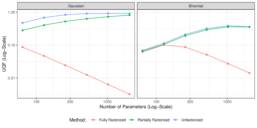
Figure 1: UQF for Simulation Study

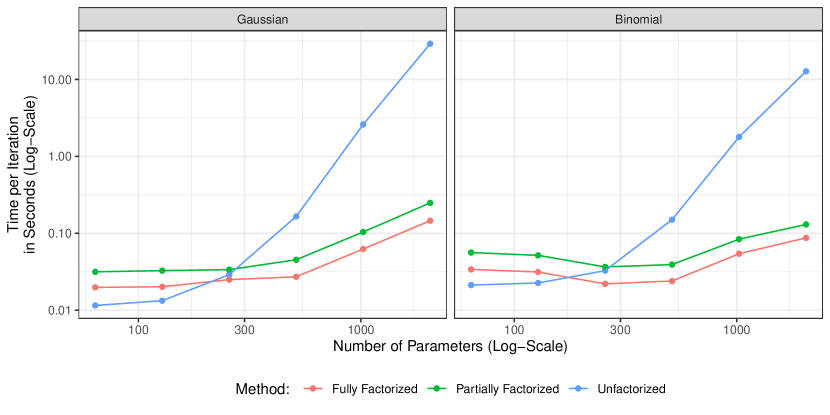
Figure 2: Time per iteration for Simulation Study

The simulation design violates various assumptions made in Section 6. In particular, $q(\bm{\phi})$ is updated and not kept fixed, as was done for the theoretical results both of Sections 4 and 6. Further, the design matrices are not balanced in the sense of Assumption 2. Nevertheless, the numerical results of Figure 1 are in very good qualitative accord with the theorems, see e.g. see e.g. the rate of decay of $UQF(q_{FF}^{*}(\bm{\theta})\|p(\bm{\theta}|\bm{y}))$ with dimensionality and the increase of $UQF(q_{PF,\{0\}}^{*}(\bm{\theta})\|p(\bm{\theta}|\bm{y}))$ with dimensionality. Figure 2 shows that for very small models, UF-VI is faster per iteration than either FF-VI and PF-VI; this is likely due to the specific implementation of the algorithms — e.g., “for loops” required for FF-VI and PF-VI that UF-VI avoids — that add some computational overhead. However, for larger models, the computational cost per iteration of UF-VI grows super-linearly, as expected.

7.3 Modelling voter turnout using multilevel regression and post-stratification

Multilevel Regression and Post-Stratification, commonly known as MRP (park2004mrp) is a method for small-area estimation using survey data that is increasingly popular in political science (e.g., lax2009estimation; warshaw2012district; broockman2018bias; lax2019party) and proceeds as follows. The combination of the categorical covariates in the survey define “types”, e.g., white male voters, aged 18-19, with high-school education in Pennsylvania. A model as in (1) is trained on the survey data and predicts the outcome given a “type” of respondent. Then, census data is typically used to derive the number of people of a given type in each geographic location, although see, e.g., kastellec for other possibilities. The geographic-level estimate is then obtained by taking a weighted average of the model predictions for each type using the census frequencies. ghitza propose using “deep” models that consist of many interactions between the different demographic and geographic categorical factors recorded in the survey; goplerud2023reeval discusses the advantages of these models compared to other machine learning approaches for building predictive models using survey data.

goplerud2022mavb develops a framework for variational inference that implements either FF-VI or UF-VI, as discussed here, and applies it to the data in ghitza. There, it is observed that FF-VI has poor uncertainty quantification while computational cost of UF-VI becomes too large for the deeper models.

This section uses the models and design in goplerud2022mavb to examine the performance of the different VI schemes outlined in this paper. As in the earlier study, the response variable is binary and records whether a respondent voted in previous elections. It considers nine model specifications that including increasingly more complex interactions among basic categorical covariates: The first model is a simple additive model with four categorical factors — age, ethnicity, income group, and state — and the ninth model is highly complex with eighteen categorical factors (including, e.g., all two-way and three-way interactions among the original four factors). All models also include some fixed effects, see Table 7.3 for descriptions. ghitza consider both the 2004 and 2008 elections separately; we follow this but pool or average the results from each election in the following figures for simplicity. In each model, there are 4,080 “types”; in each election, they use a dataset of around 75,000 (weighted) observations.

Table 1: Description of Models

Model	Description	$\sum_{k\in\mathcal{C}}G_{k}D_{k}$	$\sum_{k\in\mathcal{U}}G_{k}D_{k}$
Model 1	Additive model (age, income, state, ethnicity)	6	64
Model 2	Adds random slopes for (continuous) income on age, state, and ethnicity	6	123
Model 3	Adds two-way interactions between age, income, and ethnicity	27	158
Model 4	Adds two-way interactions between state and demographic variables	129	719
Model 5	Adds region (e.g., “South”) and interactions between region and demographics	139	784
Model 6	Adds three-way interaction between age, income, and ethnicity	139	864
Model 7	Adds three-way interaction between state, ethnicity, and income	139	1884
Model 8	Adds three-way interaction between state, ethnicity, and age	139	2700
Model 9	Adds three-way interaction between state, income, and age	139	3720

For the partially factorized approximations, we follow the principle suggested in Section 6.1 and include fixed and, when interactions exist, the corresponding main effects in $\mathcal{C}$. We compare the variational approximations against a “gold standard” posterior sampled using HMC. Paralleling the analyses in Section 7.2, we present two sets of results to illustrate the relative performance of the methods. Figure 3 shows, as predicted by the theory, that the $UQF$ for FF-VI is close to zero for all models whereas that for PF-VI remains drastically larger even for the most complex models. We also see that adding to $\mathcal{C}$ the main effects makes a significant difference in terms of $UQF$ when there are interactions in the model (i.e. for models 3 to 9), as predicted by the theory.

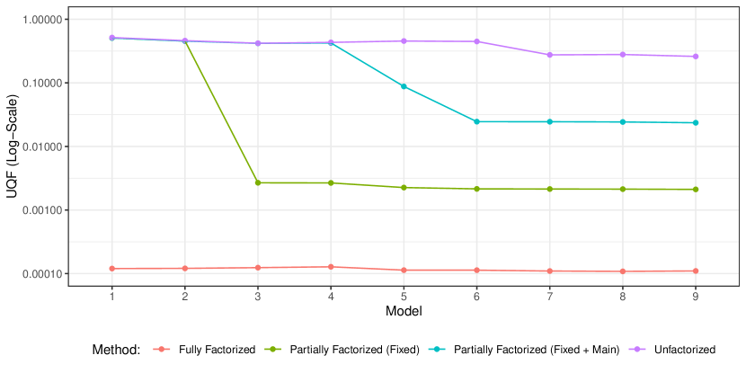
Figure 3: $UQF$ for Voter Turnout

Second, we consider the accuracy of the variational approximations on key quantities of interest to applied researchers. One is state-level estimates of turnout that are computed using post-stratification. Another is the linear predictor for each of the 4,080 “types.” Figure 4 provides boxplots of these estimated accuracy scores across all parameters of interest and datasets. We see that, for the state-level MRP estimates, PF-VI with main effects are included in $\mathcal{C}$ performs well even for the most complex models — basically on pair with UF-VI, while FF-VI and PF-VI with $\mathcal{C}=\{0\}$ struggle for models from 4 to 9. For the linear predictor, the results are roughly analogous, with the only exception that PF-VI with main effects included in $\mathcal{C}$ is accurate for most “types” for models from 1 to 6, while a tail of inaccurate “types” appears for models 7 to 9.

Exploring this phenomenon suggests that this tail for PF-VI typically corresponds to rare types, i.e. cells in the contingency table with very few observations. As these observations are downweighted during the post-stratification stage, it is still possible to see the high levels of accuracy found in the left panel. On the other hand, we have empirically found that FF-VI — in addition to underestimating the posterior variance for rare “types” — tends to dramatically overestimate the variance of common “types”, which in turns contributes to the low accuracy on the left panel.

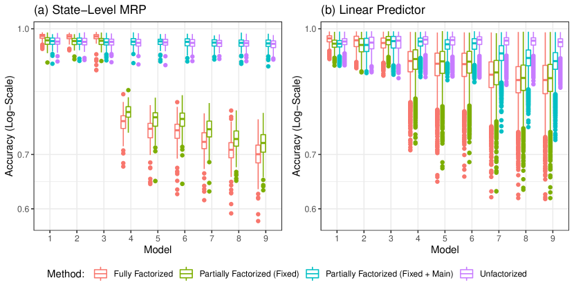
Figure 4: Accuracy of Estimates for Voter Turnout

Overall, the results of this section supports the claim that, for the majority of models and quantities of interests, PF-VI with $\mathcal{C}$ chosen as proposed in Section 6.1 achieves an accuracy comparable to UF-VI but at a fraction of computational time — around three minutes for PF-VI, including interactions, versus around forty minutes for UF-VI.

8 Future research directions

This paper leaves open many directions for future research. In terms of theoretical questions, possible work might analyse the UQF of PF-VI for GLMMs beyond the specific settings examined in Section 6, e.g. examining the case of $K>2$ factors. We expect the proof techniques of Section 6 to be also applicable to provide an explicit theoretical comparison of the computational-accuracy trade-off of PF-VI versus the one of previously proposed approaches discussed in Section 3.2, such as blocking (menictas2023streamlined). More generally, it would be interesting to extend the results on the accuracy and convergence duality for VI of Section 4 to more general settings, such as log-concave distributions. On the applied side, developing a more data-driven approach for choosing $\mathcal{C}$ given some constraint on its size could be useful for extending the model to settings with other types of hierarchical terms, e.g., those used in generalized additive models.

In this article, we have focused on the use of PF-VI for full Bayesian inference, but we expect the techniques and results discussed in this article to extend — with appropriate modifications — to different inferential frameworks, e.g., for restricted maximum likelihood using a variational EM algorithm or methods based on Laplace approximations. Also, while in this article we have focused on the practically important cases of Gaussian and binomial likelihoods, we expect PF-VI techniques to extend more broadly to other likelihood functions using, for example, non-conjugate variational message passing (knowles2011non; wand2014fully; ncp-vi) or Gaussian variational approximations (ormerod2012gva). We leave a more detailed exploration of such extensions to future work. Finally, we also note that this methodology can be used with more flexible priors on $\bm{\Sigma}_{k}$; goplerud2023reeval found that using less informative priors improves the statistical properties of the resultant inference but it considerably slowed convergence of FF-CAVI. We anticipate that this situation can also be improved using PF-CAVI.

The PF-VI methodology implemented in the accompanying R package vglmer. The package includes a slightly more flexible factorization scheme than that described in Sections 3 and 5, where $\bm{\theta}_{\mathcal{C}}$ included all levels of a specific factor $k\in\mathcal{C}$. In the accompanying software, it is also possible to include only some levels $g$ of a factor $k$ in $\mathcal{C}$. Our paper only considers the “all or none” strategy for both notational and conceptual simplicity, as this level of generality was sufficient to obtain satisfactory results. Additional acceleration techniques to improve estimation (e.g., parameter-expanded variational inference; see goplerud2023reeval for examples) can also be used alongside PF-CAVI if desired.

Appendix

Proofs of Section 4

Proof of Proposition 2

Proof.

To simplify exposition let $\bm{\Sigma},\widetilde{\bm{\Sigma}}$ be the covariance matrices of $\bm{\theta}$ under $\pi$ and $q$ respectively and $\bm{Q},\widetilde{\bm{Q}}$ the corresponding precision matrices. Given that $\widetilde{\bm{\Sigma}}$ is positive definite a square root $\widetilde{\bm{\Sigma}}^{1/2}$ is well-defined and without loss of generality we will take below the symmetric square root. Notice first that $\mathrm{Var}_{q}(\bm{\theta}^{T}\bm{v})=\bm{v}^{T}\tilde{\bm{\Sigma}}\bm{v}$, with an analogous expression for $\mathrm{Var}_{\pi}(\bm{\theta}^{T}\bm{v})$. Then, since the supremum over all $\bm{v}\in\mathbb{R}^{d}$ is the same over all vectors $\widetilde{\bm{\Sigma}}^{1/2}\bm{v}$ (due to the assumed invertibility of the matrix) we have that UQF(q ∥π) = inf_u u^T u uT~Q1/2Σ~Q1/2u= 1 / sup_u: ——u——=1 u^T ~Q^1/2 Σ ~Q^1/2 u. Recall now that for a positive definite matrix the supremum of quadratic forms over all vectors of norm 1 is its maximum eigenvalue, and that the maximum eigenvalue of a positive definite matrix is the inverse of the minimum eigenvalue of its inverse. Recall also that the eigenvalues of $\widetilde{\bm{Q}}^{1/2}\bm{\Sigma}\widetilde{\bm{Q}}^{1/2}$ are the same as those of $\widetilde{\bm{Q}}^{-1/2}\widetilde{\bm{Q}}^{1/2}\bm{\Sigma}\widetilde{\bm{Q}}^{1/2}\bm{\tilde{Q}}^{1/2}$ since this is a similarity transform. These observations lead to (2). ∎

Proof of Proposition 3

Proof.

By assumption $\pi(\bm{\theta})\equiv\mathcal{N}(\bm{\theta};\bm{\mu},\bm{Q}^{-1})$; let $\bm{\mu},\bm{Q}$ be organized according to $\mathcal{U},\mathcal{C}$, hence, e.g., $\bm{Q}_{\mathcal{UU}}$ denotes the block of the matrix corresponding to the $\theta_{k}$ for $k\in\mathcal{U}$. Since $\pi(\bm{\theta})$ is Gaussian then both $\pi(\bm{\theta}_{\mathcal{C}}|\bm{\theta}_{\mathcal{U}})$ and $\pi(\bm{\theta}_{\mathcal{U}})$ are Gaussian, the precision of the latter is given by $\bm{Q}_{\mathcal{UU}}-\bm{Q}_{\mathcal{UC}}\bm{Q}_{\mathcal{CC}}^{-1}\bm{Q}_{\mathcal{CU}}$. From the proof of Proposition 1 we recall that $q^{*}(\bm{\theta}_{\mathcal{C}}|\bm{\theta}_{\mathcal{U}})=\pi(\bm{\theta}_{\mathcal{C}}|\bm{\theta}_{\mathcal{U}})$, it is unique and is obtained after a single update, and that the CAVI iterates for $q(\bm{\theta}_{k})$, $k\in\mathcal{U}$, minimize the KL divergence between the marginal $\pi(\bm{\theta}_{\mathcal{U}})$ and its factorized approximation. It is then known (see, e.g., Chapter 10 of bishop) that for $\pi(\bm{\theta}_{\mathcal{U}})$ Gaussian, $\{q^{*}(\bm{\theta}_{k})\}$ is unique and is Gaussian with mean $\bm{\mu}_{k}$ and precision the $k$’th diagonal block of $\bm{Q}_{\mathcal{UU}}-\bm{Q}_{\mathcal{UC}}\bm{Q}_{\mathcal{CC}}^{-1}\bm{Q}_{\mathcal{CU}}$; let $\widetilde{\bm{Q}_{\mathcal{UU}}}$ denote the block-diagonal matrix that contains these precision matrices. Therefore, $q^{*}(\bm{\theta}_{\mathcal{C}},\bm{\theta}_{\mathcal{U}})$ is unique, it is Gaussian with mean $\bm{\mu}$ and precision matrix with the same blocks as $\bm{Q}$ with the exception of that $\widetilde{\bm{Q}_{\mathcal{UU}}}$ replaces $\bm{Q}_{\mathcal{UU}}$.

By appealing to Proposition 2 and its proof, we get that $UQF(q^{*}\|\pi)$ is the smallest eigenvalue of the product of the precision under $\pi$ and the covariance under $q^{*}$. A careful calculation using both of the two standard expressions for the inverse of a block matrix (the one that inverts the top left and the one that inverts the bottom right) shows that the product is a block lower triangular matrix with diagonal elements the identity matrix for the $\mathcal{CC}$-block and (Q_UU - Q_UCQ_CC^-1 Q_CU)(~Q_UU - Q_UCQ_CC^-1 Q_CU)^-1, for the $\mathcal{UU}$-block. We can recognize the second term in the product as $\mathrm{Cov}_{q^{*}}(\bm{\theta}_{\mathcal{U}})$, as obtained by block-wise inversion. However, we know from the factorization and the optimality of mean field for Gaussian that this is simply $\widetilde{\bm{Q}_{\mathcal{UU}}}^{-1}$ since the covariance under $q^{*}$ is block-diagonal. Therefore, the $\mathcal{UU}$-block can be expressed generically as $\bm{P}\widetilde{\bm{P}}^{-1}$ for $\bm{P}$ positive definite organized in $K$ blocks and $\widetilde{\bm{P}}$ block-diagonal containing the diagonal blocks of $\bm{P}$. Therefore, the matrix that determines $UQF$ will have the eigenvalue 1 with multiplicity $|\mathcal{C}|$ and the rest of its eigenvalues are those of $\bm{P}\widetilde{\bm{P}}^{-1}$. We now show that the minimum eigenvalue of such a matrix is less than 1.

First, note that due to a similarity transformation the eigenvalues of $\bm{P}\widetilde{\bm{P}}^{-1}$ are the same as those of $\widetilde{\bm{P}}^{-1/2}\bm{P}\widetilde{\bm{P}}^{-1/2}$. This is a matrix with $|\mathcal{U}|$ diagonal blocks that are identity matrices. Consider a vector $\bm{w}$ with constant entries on the 1st block and 0 everywhere else, normalized to have norm 1. Then λ_min(~P^-1/2P~P^-1/2)= inf_v:v^T v=1 v^T ~P^-1/2P~P^-1/2 v ≤w^T ~P^-1/2P~P^-1/2 w = w^T w = 1 .

∎

Random-scan PF-CAVI

Theorem 1 analyzes the random scan version of PF-CAVI and for completeness we provide here its description. We focus on the variational problem defined in Assumption 1. For this problem, as obtained in the proof of Proposition 1, $q^{*}(\bm{\theta}_{\mathcal{C}}|\bm{\theta}_{\mathcal{U}})=\pi(\bm{\theta}_{\mathcal{C}}|\bm{\theta}_{\mathcal{U}})$ and is found after a single update. Therefore, the algorithm updates this term only once and randomly scan through the other terms to perform updates. In order to match computational costs between $T$ iterations of random and deterministic scan versions, Algorithm 2 performs $|\mathcal{U}|T$ random-scan updates instead of $T$. Equivalently, at each random-scan update in Algorithm 2 we increase time by $1/K$.

Input: target distribution $\pi(\bm{\theta})$; sets $\mathcal{C}\subseteq\{0,\ldots,K\}$ and $\mathcal{U}=\{0,\ldots,K\}\setminus\mathcal{C}$

Initialize $q_{0}(\bm{\theta}_{k})$ for $k\in\mathcal{U}$

Set $t\leftarrow 0$

while $t<T$ do

     Pick $k$ uniformly at random from $\mathcal{U}$

     Set $q_{t+1/K}(\bm{\theta}_{k^{\prime}})=q_{t}(\bm{\theta}_{k^{\prime}})$ for $k^{\prime}\in{\mathcal{U}}\backslash\{k\}$

     Set $q_{t+1/K}(\bm{\theta}_{k})\propto\exp\left\{\mathbb{E}_{q_{t}(\bm{\theta}_{\mathcal{U}\backslash k})}[\log\pi(\bm{\theta}_{\mathcal{U}})]\right\}$

     Set $t\leftarrow t+1/K$

end while

Output $q_{T}(\bm{\theta})=\pi(\bm{\theta}_{\mathcal{C}}|\bm{\theta}_{\mathcal{U}})\left[\prod_{k\in\mathcal{U}}q_{T}(\bm{\theta}_{k})\right]$

Algorithm 2 Random-scan PF-CAVI targeting $\pi$

Proof of Theorem 1

Proof.

For given $t$, let $s=|\mathcal{U}|t$, and let $q_{s}(\bm{\theta})=\pi(\bm{\theta}_{\mathcal{C}}|\bm{\theta}_{\mathcal{U}})q_{s}(\bm{\theta}_{\mathcal{U}})$ be the density returned after $|\mathcal{U}|t$ iterations of random scan CAVI, where $q_{s}(\bm{\theta}_{\mathcal{U}})=\left[\prod_{k\in\mathcal{U}}q_{s}(\bm{\theta}_{k})\right]$. Denoting by $q^{*}(\bm{\theta})$ and $q^{*}(\bm{\theta}_{\mathcal{U}})$ the corresponding optimal at convergence, the proof of Proposition 3 shows that $UQF(q^{*}(\bm{\theta})\|\pi(\bm{\theta}))=UQF(q^{*}(\bm{\theta}_{\mathcal{U}})\|\pi(\bm{\theta}_{\mathcal{U}}))$. It also follows easily that $KL(q_{s}(\bm{\theta})|\pi(\bm{\theta}))=KL(q_{s}(\bm{\theta}_{\mathcal{U}})|\pi(\bm{\theta}_{\mathcal{U}}))$ with analogous equality for the optimized densities. Therefore, for the rest of the proof it suffices to focus on the algorithm that approximates $\pi(\bm{\theta}_{\mathcal{U}})$ by the mean field $\prod_{k\in\mathcal{U}}q(\bm{\theta}_{k})$ using a random scan CAVI.

Given the assumption that $\pi(\bm{\theta})$ is Gaussian, we have that $\pi(\bm{\theta}_{\mathcal{U}})$ is Gaussian and let $\bm{\mu},\bm{Q}$ denote its mean and precision, and let $\bm{b}=\bm{Q\mu}$. Then, it is s well known (see for example Chapter 10 of bishop) that when updating the $k$’th term in the approximation, the coordinate-wise optimum is $\mathcal{N}(\bm{m}_{k},(\bm{Q}_{k,k})^{-1})$, where the mean depends on the means of all other densities via the relation

$$\bm{Q}_{k,k}\bm{m}_{k}=\bm{Q}_{k,k}\bm{m}_{k}-\sum_{\ell}\bm{Q}_{k,\ell}\bm{m}_{\ell}+\bm{b}_{k}\,.$$

The following basic considerations allow us to simplify the study of convergence of CAVI in this context. First, note that convergence of CAVI is precisely that of the convergence of the means $\bm{m}^{(k)}$ to their stationary point, since the corresponding precision matrices converge after one iteration to their limit. Second, the convergence of the linear dynamical system given above does not depend on $\bm{b}$ and remains the same if we do the coordinate-wise reparameterisation $\bm{m}_{k}\to\bm{Q}_{k,k}^{1/2}\bm{m}_{k}$. When taking also into account the first expression for $UQF$ in Proposition 2 we conclude that without loss of generality in the rest of the proof we can take $\bm{\mu}=\bm{0}$ and that $\bm{Q}^{(k,k)}=\bm{I}$ for each block $k$. Notice then that

$$UQF(q^{*}\|\pi)=\lambda_{min}(\bm{Q})<1,$$

where the upper bound is due to Proposition 3. Letting $\bm{m}_{t}$ be the vector of means after $s$ iterations, a direct calculation yields that

$$V(q^{*}\|\pi)-V(\pi\|q_{s})={1\over 2}\bm{m}_{s}^{T}\bm{Q}\bm{m}_{s}\,.$$

Under the above considerations, we can now focus on obtaining convergence bounds for the random scan coordinate descent for minimizing $V(\bm{m})=\bm{m}^{T}\bm{Q}\bm{m}/2$, with $\bm{m}$ organized in $|\mathcal{U}|$ blocks and $\bm{Q}$ having identity diagonal blocks, with $\bm{m}_{t}$ denoting the vector after $t$ random coordinate minimizations.

Let $\mathcal{F}_{s}$ be the filtration generated by $I_{1},\ldots,I_{s}$. Then, a careful calculation obtains the following equality, whereas the inequality is a basic eigenvalue bound:

$$\mathbb{E}[V(\bm{m}_{s+1})\mid\mathcal{F}_{s}]=V(\bm{m}_{s})-{1\over|\mathcal{U}|}{1\over 2}\bm{m}_{s}^{T}\bm{Q}^{2}\bm{m}_{s}\leq\left(1-{1\over|\mathcal{U}|}\lambda_{min}(\bm{Q})\right)V(\bm{m}_{s})\,,$$

from which we directly obtain

$$\mathbb{E}[V(\bm{m}_{|\mathcal{U}|t}]\leq\left(1-{\lambda_{min}(\bm{Q})\over|\mathcal{U}|}\right)^{|\mathcal{U}|t}V(\bm{m}_{0})\,.$$

For the lower bound, note first that

$$\mathbb{E}[\bm{m}_{s+1}\mid\mathcal{F}_{s}]=(\bm{I}-\bm{Q}/|\mathcal{U}|)\bm{m}_{s}\,,$$

an implication of which is that if $\bm{m}_{0}$ is an eigenvector of $\bm{Q}$ with eigenvalue $\lambda$ then $\mathbb{E}[\bm{m}_{s+1}]=(1-\lambda/|\mathcal{U}|)^{s+1}\bm{m}_{0}$. Since for positive semi-definite $\bm{Q}$, $V(\bm{m})$ is a convex function, we can apply Jensen’s inequality to obtain:

$$\mathbb{E}[V(\bm{m}_{|\mathcal{U}|t})]\geq\mathbb{E}[\bm{m}_{|\mathcal{U}|t}]^{T}\bm{Q}\mathbb{E}[\bm{m}_{|\mathcal{U}|t}]=(1-\lambda/|\mathcal{U}|)^{2|\mathcal{U}|t}V(\bm{m}_{0})\,.$$

The proof is concluded by taking $\bm{m}_{0}$ to be the eigenvector that corresponds to $\lambda_{min}(\bm{Q})$. ∎

Proofs of Section 6

Throughout these proofs we use the following definitions. We define a block matrix $\bm{N}$ that contains the weighted counts $n_{g,h}^{(k,\ell)}$ defined in (24), organized according to the numbering of the factors and their levels. For $\bm{Q}$ and $\widetilde{\bm{Q}}$ the precision matrices under the target and the variational approximation, we define

$$\bar{\bm{Q}}=\widetilde{\bm{Q}}^{-1/2}\bm{Q}\widetilde{\bm{Q}}^{-1/2}.$$ (29)

When the target is Gaussian, $\mathcal{C}=\emptyset$ implies that $\widetilde{\bm{Q}}$ coincides with $\bm{Q}$ on diagonal blocks and it is zero elsewhere, which in turn implies that $\bar{\bm{Q}}$ is a matrix whose diagonal blocks are identity matrices. The following generic Lemma is used to prove Theorem 2.

Lemma 1.

Consider $\bm{Q},\widetilde{\bm{Q}},\bar{\bm{Q}}$ as in (29) and vectors $\bm{v}_{k},\bm{v}_{\ell}$ for $k\neq\ell$ such that $\bm{v}_{k}$ has only non-zero elements in the $k$-th block, and $\bm{v}_{\ell}$ accordingly. Then:

$$UQF(q\|\pi)\leq 1-{\bm{v}_{k}^{T}\bar{\bm{Q}}\bm{v}_{\ell}\over\|\bm{v}_{k}\|\|\bm{v}_{\ell}\|}\,.$$

Proof.

For $\bm{u}_{k}=\bm{v}_{k}/\|\bm{v}_{k}\|^{2}$ and $\bm{u}_{\ell}$ defined accordingly, note that they are orthogonal and normalized to 1. Consider the $2\times 2$ matrix

$$\bm{C}=\left(\begin{array}[]{c}\bm{u}_{k}^{T}\\ \bm{u}_{\ell}^{T}\end{array}\right)\bar{\bm{Q}}(\bm{u}_{k}\quad\bm{u}_{\ell})\,.$$

By construction $C_{ii}=1$ for $i=1,2$ and $\bm{C}$ inherits positive definitess from $\bm{\bar{Q}}$. Then:

$$UQF(q\|\pi) =\lambda_{min}(\bar{\bm{Q}})\leq\min_{\gamma_{1},\gamma_{2}}{(\gamma_{1}\bm{u}_{k}+\gamma_{2}\bm{u}_{\ell})^{T}\bar{\bm{Q}}(\gamma_{1}\bm{u}_{k}+\gamma_{2}\bm{u}_{\ell})\over\gamma_{1}^{2}+\gamma_{2}^{2}}$$

$$=\min_{\bm{\gamma}}{\bm{\gamma}^{T}\bm{C}\bm{\gamma}\over\|\bm{\gamma}\|^{2}}=\lambda_{min}(\bm{C})=1-C_{12}\,.$$

Replacing by $\bm{v}_{k},\bm{v}_{\ell}$ completes the proof. ∎

Proof of Theorem 2

Proof.

Directly from Proposition 4 for $\mathcal{C}=\emptyset$, we obtain that the precision of $\pi(\bm{\theta})$, denoted by $\bm{Q}$ below, is

$$\bm{Q}_{k,k} =T_{k}\bm{I}+\mathrm{diag}[(n_{g}^{(k)})_{g=1:G_{k}}],\quad\quad\bm{Q}_{k,\ell}=\bm{N}_{k,\ell},\quad k,\ell>0,k\neq\ell$$ (30)

$$\quad Q_{0,0} =\delta,\quad\bm{Q}_{0,k}=(n_{g}^{(k)})_{g=1:G_{k}},k>0\,,$$ (31)

where $\delta=\sum_{g=1}^{G_{k}}n_{g}^{(k)}=n\bar{D}$. It is well known (see also proof of Theorem 1) that for such target the optimized approximation of the variational problem in (13) is Gaussian with precision $\widetilde{\bm{Q}}$ given by the diagonal blocks of $\bm{Q}$ above. Then, for $\bar{\bm{Q}}$ as in (29), a direct calculation yields that

$$\bar{\bm{Q}}_{k,k} =\bm{I},k>0,\quad\bar{Q}_{0,0}=1,\quad(\bar{Q}_{k,\ell})_{g,h}=b_{g}^{(k)}b_{h}^{(\ell)}n^{(k,\ell)}_{g,h},\quad(\bar{Q}_{0,k})_{g}={b_{g}^{(k)}\over\sqrt{\delta}}n_{g}^{(k)},k,\ell>0\,,$$

for

$$b_{g}^{(k)}=\sqrt{1\over T_{k}+n^{(k)}_{g}}\,,$$

and where $(\bar{Q}_{k,\ell})_{g,h}$ denotes the $(g,h)$ element of the block $\bar{\bm{Q}}_{k,\ell}$. Consider now $\bm{v}_{k},k>0$ a vector with 0’s except for positions on the $k$’th block, where the $g$’th position in the $k$th block takes the value $1/b_{g}^{(k)}$, and $\bm{v}_{0}$ which is non-zero only the 0’th position and takes the value $\sqrt{\delta}$. Then note that:

$$\bm{v}_{0}\bar{\bm{Q}}\bm{v}_{k} =\sum_{g=1}^{G_{k}}n_{g}^{(k)},\quad\|\bm{v}^{(0)}\|=\sqrt{\sum_{i}\delta_{i}},\quad\|\bm{v}^{(k)}\|=\sqrt{G_{k}T_{k}+\sum_{g=1}^{G_{k}}n_{g}^{(k)}}\,.$$

Appealing to Lemma 1 we obtain the result. ∎

Proof of Theorem 3

We first state a preliminary lemma.

Lemma 2.

Let $\bm{M}=(\bm{M}_{k,\ell})_{k,\ell=1,2}$ be a symmetric positive definite $2\times 2$ block matrix, and

$$\bm{C}=\left(\begin{array}[]{cc}\bm{M}_{1,1}&\bm{0}\\ \bm{0}&\bm{M}_{2,2}\end{array}\right)^{-1/2}\left(\begin{array}[]{cc}\bm{M}_{1,1}&\bm{M}_{1,2}\\ \bm{M}_{2,1}&\bm{M}_{2,2}\end{array}\right)\left(\begin{array}[]{cc}\bm{M}_{1,1}&\bm{0}\\ \bm{0}&\bm{M}_{2,2}\end{array}\right)^{-1/2}\,,$$

Then, the minimum modulus eigenvalue of $\bm{C}$ is λ_min(C)=1-ρ(M_1,1^-1 M_1,2 M_2,2^-1M_2,2) where $\rho(A)$ denotes the largest modulus eigenvalue of a matrix $A$.

Proof.

Let $d_{1}$ and $d_{2}$ be the dimensionality of $\bm{M}_{1,1}$ and $\bm{M}_{2,2}$, respectively. Assume $d_{2}\geq d_{1}$ without loss of generality. We have C = I_d_1+d_2+~C ,   ~C= ( 0_d_1AA^T0_d_2) where $\bm{A}=\bm{M}_{1,1}^{-1/2}\bm{M}_{1,2}\bm{M}_{2,2}^{-1/2}$, $\bm{I}_{d}$ denote a $d\times d$ identity matrix and $\bm{0}_{d}$ denotes a $d\times d$ matrix of zeros. It follows that the spectrum of $\bm{C}$ coincides with the one of $\tilde{\bm{C}}$ traslated by $+1$. The matrix $\tilde{\bm{C}}$ can be interpreted as the adjacency matrix of a bipartite graph and it can be easily shown that its spectrum coincides with the union of $1$, with multiplicity $d_{2}-d_{1}$, the singular values of $A$ and the singular values of $A$ with negative sign, see e.g. brito2022spectral. It follows that $\rho(\bm{C})=1-\sqrt{\rho(\bm{A}\bm{A}^{T})}$, where we also used that the singular values of $A$ have modulus less than $1$, which follows from $\bm{A}=\bm{M}_{1,1}^{-1/2}\bm{M}_{1,2}\bm{M}_{2,2}^{-1/2}$ and the positive definiteness of $\bm{Q}$. To conclude, note that ρ(AA^T)= ρ(M_1,1^-1/2M_1,2M_2,2^-1M_1,2M_2,2^-1/2) = ρ(M_1,1^-1M_1,2M_2,2^-1M_1,2) . ∎

Proof of Theorem 3.

By Proposition 4 $\pi(\bm{\theta})$ is Gaussian. Thus we can apply the proof of Proposition 3 to deduce $UQF(q^{*}(\bm{\theta})\|\pi(\bm{\theta}))=UQF(q^{*}(\bm{\theta}_{\mathcal{U}})\|\pi(\bm{\theta}_{\mathcal{U}}))$. By Proposition 2

$$UQF(q^{*}(\bm{\theta}_{\mathcal{U}})\|\pi(\bm{\theta}_{\mathcal{U}}))=\lambda_{min}(\mathrm{Cov}_{q^{*}}(\bm{\theta}_{\mathcal{U}})^{1/2}\mathrm{Cov}_{\pi}(\bm{\theta}_{\mathcal{U}})^{-1}\mathrm{Cov}_{q^{*}}(\bm{\theta}_{\mathcal{U}})^{1/2})\,.$$

Denoting the precision matrix of $\pi(\bm{\theta}_{\mathcal{U}})$ as a $2\times 2$ block matrix M=Cov_π(θ_U)^-1=( M_1,1M_1,2M_2,1M_2,2