Renormalon-based resummation of Bjorken polarised sum rule in holomorphic QCD

Abstract

Approximate knowledge of the renormalon structure of Bjorken polarised sum rule (BSR) ${\overline{\Gamma}}_{1}^{{\rm p-n}}(Q^{2})$ leads to the corresponding BSR characteristic function that allows us to evaluate the leading-twist part of BSR. In our previous work pPLB , this evaluation (resummation) was performed using perturbative QCD (pQCD) coupling $a(Q^{2})\equiv\alpha_{s}(Q^{2})/\pi$ in specific renormalisation schemes. In the present paper, we continue this work, by using instead holomorphic couplings [$a(Q^{2})\mapsto{\mathcal{A}}(Q^{2})$] that have no Landau singularities and thus require, in contrast to the pQCD case, no regularisation of the resummation formula. The $D=2$ and $D=4$ terms are included in the Operator Product Expansion (OPE) of inelastic BSR, and fits are performed to the available experimental data in a specific interval $(Q^{2}_{\rm min},Q^{2}_{\rm max})$ where $Q^{2}_{\rm max}=4.74\ {\rm GeV}^{2}$. We needed relatively high $Q^{2}_{\rm min}\approx 1.7\ {\rm GeV}^{2}$ in the pQCD case since the pQCD coupling $a(Q^{2})$ has Landau singularities at $Q^{2}\lesssim 1\ {\rm GeV}^{2}$. Now, when holomorphic (AQCD) couplings ${\mathcal{A}}(Q^{2})$ are used, no such problems occur: for the $3\delta$AQCD and $2\delta$AQCD variants the preferred values are $Q^{2}_{\rm min}\approx 0.6\ {\rm GeV}^{2}$. The preferred values of $\alpha_{s}$ in general cannot be unambiguously extracted, due to large uncertainties of the experimental BSR data, although the fit with $2\delta$AQCD and the $D=2$ term included suggests $\alpha_{s}^{{\overline{\rm MS}}}(M_{Z}^{2})\approx 0.1181$. At a fixed value of $\alpha_{s}^{{\overline{\rm MS}}}(M_{Z}^{2})$, the values of the $D=2$ and $D=4$ residue parameters are determined in all cases, with the corresponding uncertainties.

I Introduction

We analyse in this work the inelastic polarised Bjorken sum rule (BSR) ${\overline{\Gamma}}_{1}^{{\rm p-n}}(Q^{2})$ BjorkenSR ; BSR70 , which is the difference of the spin-dependent structure functions of proton and neutron integrated over the $x$-Bjorken parameter range $0<x<1$. Its Operator Product Expansion (OPE) has a relatively simple form, because it is an isovector and spacelike quantity.

Experimental results for ${\overline{\Gamma}}_{1}^{{\rm p-n}}(Q^{2})$, though often with significant statistical and systematic uncertainties, are available from various experiments: CERN CERN , DESY DESY , SLAC SLAC , and from various experiments at the Jefferson Lab JeffL1 ; JeffL2 ; JeffL3 ; JeffL4 ; JeffL5 . These experimental results are based on the measured values of the spin-dependent structure functions over various values of Bjorken $x$, and over various values of $Q^{2}$ in the wide range $0.02\ {\rm GeV}^{2}<Q^{2}<5\ {\rm GeV}^{2}$ where $q^{2}\equiv-Q^{2}$ is the squared momentum transfer.

On the other hand, the considered inelastic BSR ${\overline{\Gamma}}_{1}^{{\rm p-n}}(Q^{2})$ is evaluated theoretically by using OPE that is usually truncated at the dimension $D=2$ ($\sim 1/Q^{2}$) or $D=4$ ($\sim 1/(Q^{2})^{2}$) term. The leading-twist ($D=0$) term has the canonical QCD part $d(Q^{2})$ which is in general evaluated as a truncated perturbation series (TPS) in powers of the pQCD coupling $a(Q^{2})=\alpha_{s}(Q^{2})/\pi$. The values of the first four expansion coefficients (i.e., up to $\sim a^{4}$) have been calculated exactly GorLar1986 ; LarVer1991 ; BaiCheKu2010 , and the value of the coefficient at $a^{5}$ can be estimated. In this way, the mentioned OPE expression is then fitted to the experimental data, and the values of the OPE coefficient of the $D=2$ term, and possibly of the $D=4$ term, can be extracted. This pQCD OPE approach, or specific variants of it, has been followed in the works ABFR ; JeffL1 ; JeffL2 ; JeffL4 ; ACKS ; KoMikh ; BSRPMC .

The described approaches of theoretical evaluation do not involve direct resummations in the canonical QCD part of BSR, $d(Q^{2})$ Analyses of BSR were also performed in the approaches that use holomorphic QCD (AQCD) running couplings $a(Q^{2})\mapsto{\mathcal{A}}(Q^{2})$ (i.e., free of Landau singularities) in $d(Q^{2})$, enabling the evaluation of $d(Q^{2})$ even at lower $Q^{2}\lesssim 1\ {\rm GeV}^{2}$ ACKS . However, even in those AQCD cases, the series for $d(Q^{2})$ were truncated. Actually, we know that $d(Q^{2})$ of BSR has the expansion coefficients $d_{n}$ (at $a^{n+1}$) that grow very fast with increasing $n$, approximately as $d_{n}\sim n!(\beta_{0}/p)^{n}$ with $p=1$ (due to the leading infrared renormalon close to the origin, $u=p=1$), which indicates that truncation of $d(Q^{2})$, at $\sim a^{4}$ or $\sim a^{5}$, may miss important contributions.

In our previous work pPLB , we evaluated the QCD canonical part $d(Q^{2})$ of BSR by performing a renormalon-based resummation. The extension of the $d(Q^{2})$ expansion to higher powers of $a$ was performed by a renormalon-based approach. The latter approach allows us to construct a characteristic function of $d(Q^{2})$ and enables us to perform resummation in a form of integration that involves $a(Q^{{}^{\prime}2})$ over the entire range of spacelike scales $0<Q^{{}^{\prime}2}<\infty$. In pPLB the pQCD coupling $a(Q^{{}^{\prime}2})$ was used in the resummation formula and the fits of the corresponding (truncated) OPE to the experimental data were performed. The pQCD coupling has Landau singularities (in the range $0<Q^{{}^{\prime}2}<1\ {\rm GeV}^{2}$), and hence a regularisation of the resummed result was needed. In the present work, which can be regarded as a continuation of our previous work pPLB , we perform the resummation of $d(Q^{2})$ instead by using holomorphic (analytic, AQCD) couplings ${\mathcal{A}}(Q^{{}^{\prime}2})$. These running couplings have no Landau singularities, and thus no regularisation is needed. Subsequently, we perform fits with the corresponding (truncated) OPE for BSR ${\overline{\Gamma}}_{1}^{{\rm p-n}}(Q^{2})$ with the experimental data.

In Sec. II we summarise some of the theoretical aspects of the approach, though we refer for details to our previous works renmod ; pPLB . In Sec. III we present the numerical results of the various evaluations of the canonical part of BSR, $d(Q^{2})$, for the two applied types of the holomorphic (AQCD) coupling. In particular, we explore numerical behaviour of $d(Q^{2})$ when it is either resummed, or has a form of approximants based on truncated information, for these AQCD coupling. We then use the resummed AQCD results for $d(Q^{2})$ in Sec. IV to evaluate the (truncated) OPE of BSR ${\overline{\Gamma}}_{1}^{{\rm p-n}}(Q^{2})$ and fit it to the experimental data, and thus we extract the values of the OPE $D=2$ and $D=4$ coefficients, for the used two types of the AQCD coupling. In Sec. IV we also compare the obtained results with those of Ref. pPLB where pQCD coupling is used. Finally, in Sec. V we discuss the obtained numerical results, and summarise the work. Some formal details used in this work are given in Appendices A-B.

II Theoretical expressions

In this Section we only summarise briefly the final results of the formalism explained in general in Ref. renmod and, when applied to BSR in particular, in Ref. pPLB .

The theoretical OPE expression for the inelastic BSR ${\overline{\Gamma}}_{1}^{{\rm p-n}}(Q^{2})$, truncated at the dimension $D=4$ term ($\sim 1/(Q^{2})^{2}$), has the form

$${\overline{\Gamma}}_{1}^{{\rm p-n},\rm{OPE}}(Q^{2}) = {\Big{|}}\frac{g_{A}}{g_{V}}{\Big{|}}\frac{1}{6}\left[1-d(Q^{2})-\delta d(Q^{2})_{m_{c}}\right]$$ (1)

$$+ \frac{M_{N}^{2}}{9}\frac{\left[(a_{2}^{{\rm p-n}}+4d_{2}^{{\rm p-n}})+4{\bar{f}}_{2}\;{a}(Q^{2})^{{k_{1}}}\right]}{Q^{2}}+\frac{\mu_{6}}{(Q^{2})^{2}}.$$

Here $Q^{2}=-q^{2}$ and $q^{2}=(q^{0})^{2}-{\vec{q}}^{2}$ is the square of the transferred DIS momentum; $|g_{A}/g_{V}|$ is the ratio of the nucleon axial charge, and we take the value $|g_{A}/g_{V}|=1.2754$ PDG2023 . In the $D=2$ term, $k_{1}=32/81$ Kawetal1996 is the anomalous dimension of the $D=2$ operator; $M_{N}=0.9389$ GeV is the nucleon mass, and $(a_{2}^{{\rm p-n}}+4d_{2}^{{\rm p-n}})\approx 0.063$ is a combination of the twist-2 target correction and of a twist-3 matrix element. The quantity $d(Q^{2})$ is the canonical $N_{f}=3$ massless QCD contribution whose power expansion in terms of the (pQCD) coupling $a(Q^{2})\equiv\alpha_{s}(Q^{2})/\pi$ is

$$d(Q^{2})_{\rm pt} = a(Q^{2})+d_{1}a(Q^{2})^{2}+d_{2}a(Q^{2})^{3}+d_{3}a(Q^{2})^{4}+{\cal O}(a^{5}),$$ (2)

The first coefficients $d_{j}$ ($j=0,1,2,3$) are exactly known and were obtained in the $\overline{\rm MS}$ scheme in GorLar1986 ; LarVer1991 ; BaiCheKu2010 , while the next coefficient $d_{4}$ can be estimated by the effective charge (ECH) method KatStar , and its value in the 5-loop $\overline{\rm MS}$ scheme is $d_{4}^{{\overline{\rm MS}}}=1557.4$. We will take $d_{4}^{\overline{\rm MS}}\approx 1557.4\pm 32.8$, cf. pPLB .

The term $\delta d(Q^{2})_{m_{c}}$ in Eq. (1) is the correction due to the non-decoupling of the charm mass (i.e., $m_{c}\not=\infty$ effects) Blumetal , it is $\sim a(Q^{2})^{2}$ and is written down in pPLB .

The value of the dimensionless parameter ${\bar{f}}_{2}$, and possibly of the coefficient $\mu_{6}$ at the $D=4$ OPE term, are to be determined by the fitting of the theoretical expression (1) to the BSR experimental values. Due to the lack of theoretical knowledge, $\mu_{6}$ will be considered to be $Q^{2}$-independent. The OPE (1) will be truncated either at $D=2$ or $D=4$ term.

As explained in Refs. renmod ; pPLB , the construction of the renormalon-motivated resummation is largely based on the idea of reorganising the perturbation expansion (2) of $d(Q^{2})$ in powers of $a(\mu^{2})$ into an expansion in logarithmic derivatives ${{\widetilde{a}}}_{n+1}$

$${{\widetilde{a}}}_{n+1}(\mu^{2})\equiv\frac{(-1)^{n}}{n!\beta_{0}^{n}}\left(\frac{d}{d\ln\mu^{2}}\right)^{n}{a}(\mu^{2})\qquad(n=0,1,2,\ldots),$$ (3)

leading to

$$d(Q^{2}) = a(\kappa Q^{2})+d_{1}(\kappa)a(\kappa Q^{2})^{2}+\ldots+d_{n}(\kappa)a(\kappa Q^{2})^{n+1}+\ldots$$ (4a)

$$= a(\kappa Q^{2})+{{\widetilde{d}}}_{1}(\kappa)\;{{{\widetilde{a}}}}_{2}(\kappa Q^{2})+\ldots+{{\widetilde{d}}}_{n}(\kappa)\;{{{\widetilde{a}}}}_{n+1}(\kappa Q^{2})+\ldots.$$ (4b)

Here $\kappa\equiv\mu^{2}/Q^{2}$ ($0<\kappa\lesssim 1$), where $\mu^{2}$ is a chosen renormalisation scale. This reorganisation gives us new coefficients ${\widetilde{d}}_{n}(\kappa)$ that are linear combinations of the original expansion coefficients $d_{n}(\kappa),\ldots,d_{1}(\kappa)$. It is these new coefficients ${\widetilde{d}}_{n}(\kappa)$ that play the central role in the construction of the renormalon-motivated resummation. This approach can be also interpreted as an extension of the large-$\beta_{0}$ approach of resummation of Neubert Neubert to all loops. For the large-$\beta_{0}$ structure of the BSR, see BK1993 ; Renormalons (cf. also Kat1 ; Kat2 ).

The renormalon-resummed value of the canonical part $d(Q^{2})$ is

$$d(Q^{2})_{\rm res}={\rm Re}\left[\int_{0}^{\infty}\frac{dt}{t}G_{d}(t){a}(te^{-{\widetilde{K}}}Q^{2}+i\varepsilon)\right]$$ (5)

when using the pQCD running coupling $a(\mu^{2})$, and

$$d(Q^{2})_{\rm res,AQCD}=\int_{0}^{\infty}\frac{dt}{t}G_{d}(t){{\mathcal{A}}}(te^{-{\widetilde{K}}}Q^{2}).$$ (6)

when using the holomorphic (AQCD) IR-safe running coupling ${a}(Q^{2})\mapsto{{\mathcal{A}}}(Q^{2})$, i.e., a coupling that has no Landau singularities but practically coincides with ${a}(Q^{2})$ at large $|Q^{2}|>\Lambda^{2}_{\rm QCD}$. For example, such are the 2$\delta$AQCD 2dAQCD ; 2dAQCDb or 3$\delta$AQCD couplings 3dAQCD ; 3dAQCDb . In such a case, no regularisation is needed in the resummation (6), while in the pQCD case Eq. (5) the PV-regularizarion was taken pPLB , $a(\mu^{2})\mapsto{\rm Re}\;a(\mu^{2}+i\varepsilon)$, to avoid the Landau singularities.

In the resummations (5)-(6), $G_{d}(t)$ is the characteristic function of the canonical BSR $d(Q^{2})$ renmod ; pPLB ; ACT2023 ; Castro

$$G_{d}(t)=\Theta(1-t)\pi\left[\frac{{{\widetilde{d}}}^{\rm IR}_{1}t}{\Gamma(1-{k_{1}})\ln^{{k_{1}}}(1/t)}+{{\widetilde{d}}}^{\rm IR}_{2}t^{2}\right]+\Theta(t-1)\pi\left[\frac{{{\widetilde{d}}}^{\rm UV}_{1}}{t}+\frac{{{\widetilde{d}}}^{\rm UV}_{2}}{t^{2}}\right].$$ (7)

Here, the values of the residue parameters ${{\widetilde{d}}}^{\rm IR}_{j}$ and ${{\widetilde{d}}}^{\rm UV}_{j}$ ($j=1,2$), and of the rescaling parameter ${\widetilde{K}}$ in Eqs. (5)-(6), are determined by the knowledge of the first five coefficients of the power expansion (2): $d_{0}(=1)$, $d_{1},\ldots,d_{4}$. Since the latter coefficients depend on the choice of the renormalisation scheme, so do the residue parameters and ${\widetilde{K}}$. We refer for all the details to pPLB . We note that the first two terms in $G_{d}(t)$ come from the first two IR renormalons ($u=1,2$), and the other two terms from the UV renormalons ($u=-1,-2$).

The (massless) renormalisation scheme is determined by the coefficients $c_{2}$ and $c_{3}$ that appear in the renormalisation group equation (RGE)

$$\frac{d{a}(\mu^{2})}{d\ln\mu^{2}}=-\beta_{0}a(\mu^{2})^{2}\left[1+c_{1}a(\mu^{2})+c_{2}a(\mu^{2})^{2}+c_{3}a(\mu^{2})^{3}+\ldots\right].$$ (8)

In fact, the scheme is determined by the entire set of the coefficients $c_{j}$ ($j\geq 2$) Stevenson , but we use a set of beta-functions of a specific form which has only $c_{2}$ and $c_{3}$ parameters freely adjustable pPLB and conveniently allows for an explicit solution of the pQCD running coupling $a(\mu^{2})$ in terms of the Lambert function GCIK . We vary the scheme parameters, as explained and motivated in pPLB , in a specific range

$$c_{2}=9^{+2}_{-1.4},\quad c_{3}=20\pm 15,$$ (9)

primarily in order to avoid numerical instabilities coming from strong cancellations of the the infrared (IR) renormalon contributions to the resummed value of $d(Q^{2})$. The scheme for holomorphic (AQCD) couplings ${\mathcal{A}}(\mu^{2})$ refers to the scheme of the underlying pQCD coupling $a(\mu^{2})$, cf. Appendix A.

III Evaluation of the canonical part $d(Q^{2})$

In Fig. 1 we present these resummed values $d(Q^{2})_{\rm res}$ as a function of $Q^{2}$ [Eq. (6)], when either $3\delta$AQCD or $2\delta$AQCD holomorphic coupling is used. The value of the Lambert scale of the coupling is taken to be $\Lambda_{L}=0.21745$ GeV, this corresponds to the value $\alpha_{s}^{\overline{\rm MS}}(M_{Z}^{2})=0.1179$.

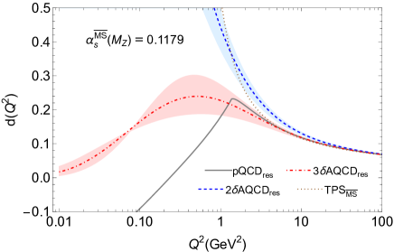
Figure 1: The resummed canonical part of BSR, $d(Q^{2})_{\rm res}$ (at $N_{f}=3$), according to Eq. (6), for the 2$\delta$ACD and 3$\delta$AQCD coupling (’$2\delta{\rm AQCD}_{\rm res}$’, ’$3\delta{\rm AQCD}_{\rm res}$’), with three hadronic threshold scales $M_{1}$ of their spectral function. For comparison, the resummed result Eq. (5) is also shown, for the pQCD coupling that is the underlying pQCD coupling of 2$\delta$ACD (’${\rm pQCD}_{\rm res}$’). Also included is the truncated perturbation series (TPS) in powers of $a=a(Q^{2})$ in the $\overline{\rm MS}$ scheme up to $\sim a^{5}$ (’${\rm TPS}_{\overline{\rm MS}}$’). All involved couplings correspond to the strength $\alpha_{s}^{\overline{\rm MS}}(M_{Z}^{2};N_{f}=5)=0.1179$, and the $d_{4}$ coefficient value corresponds to the central value of the corresponding $\overline{\rm MS}$ coefficient, $d_{4}^{\overline{\rm MS}}=1557.4$. See the text for more details.

The QCD variant $2\delta$AQCD is in the P44-scheme with $c_{2}=9.$ and $c_{3}=20.$, and the variant $3\delta$AQCD is in the (lattice-related) Lambert MiniMOM (LMM) P44-scheme MM1 ; MM2a ; MM2b ; MM3 . The construction of these QCD variants is explained in Appendix A, and they are used also in the numerical fits later on in Sec. IV. In both these holomorphic cases the strength of the underlying pQCD coupling $a(Q^{{}^{\prime}2})$ corresponds to $\alpha_{s}^{\overline{\rm MS}}(M_{Z}^{2})=0.1179$, and the threshold mass of the spectral function of the coupling ${\mathcal{A}}(Q^{{}^{\prime}2})$ has the chosen values $M_{1}=0.100,0.150$,$0.250$ GeV (the bands in the Figure correspond to the variation $M_{1}=0.150^{+0.100}_{-0.050}$ GeV). We refer to Appendix A for more details. For comparison, we also include the resummed values when pQCD coupling is used, Eq. (5), and that coupling is in the P44-scheme with $c_{2}=9.$ and $c_{3}=20.$. Further, in addition, the values of the simple truncated perturbation series (TPS, truncated at $\sim a^{5}$) in $\overline{\rm MS}$ scheme is given.

As seen in Fig. 1, the curve for the pQCD case has a (soft) kink at $Q^{2}\approx 1.44\ {\rm GeV}^{2}$. Such kinks do not appear in the cases of AQCD. The reason for the kink are the Landau singularities of the pQCD coupling $a(te^{-{\widetilde{K}}}Q^{2}+i\epsilon)$ in the integrand of the resummation (5) at low $tQ^{2}$, and the effect of these singularities becomes rather abruptly more pronounced when $Q^{2}$ has lower values ($Q^{2}\leq 1.44\ {\rm GeV}^{2}$). Furthermore, we see in Fig. 1 that the curve of $d(Q^{2})$ for 2$\delta$AQCD converges to the asymptotic (pQCD) behaviour at quite high $Q^{2}$ (in contrast to the 3$\delta$AQCD curve); this is related to the fact that the 2$\delta$AQCD coupling ${\mathcal{A}}(Q^{{}^{\prime}2})$ at low $Q^{{}^{\prime}2}$ achieves relatively high values (cf. Appendix A) and these contributions are significant in the resummation integral (6) at low $t$ values, even when $Q^{2}$ is relatively high. We remark that in Fig. 1 the pQCD TPS curve (in $\overline{\rm MS}$, with $\kappa=1$) becomes infinite at $Q^{2}\approx 0.40\ {\rm GeV}^{2}$, which is the branching point of the Landau cut of the $\overline{\rm MS}$ pQCD coupling; for $Q^{2}<0.40\ {\rm GeV}^{2}$, that TPS curve does not exist. On the other hand, the 2$\delta$AQCD and 3$\delta$AQCD curves in Fig. 1 remain finite all the way down to $Q^{2}=0$ where they reach the values of $3.70$ (when $M_{1}=0.150$ GeV) and zero, respectively.

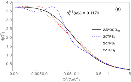
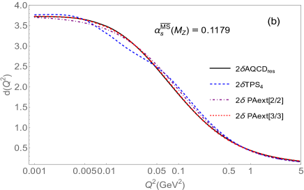
Figure 2: The resummed $d(Q^{2})$ in 2$\delta$AQCD, compared with various approximants based on truncated information about the coefficients ${\widetilde{d}}_{n}$ ($n\leq 5$): (a) the truncated series $d(Q^{2})^{[N]}_{2\delta{\rm AQCD}}$ (10) (’$2\delta{\rm TPS}_{N}$’) for $N=4,5,6$; (b) the Padé-related renormalisation scale-invariant approximants ${\cal G}_{d}^{[M/M]}(Q^{2})_{2\delta{\rm AQCD}}$ Eq. (27) (’$2\delta$PAext[M/M]’), for $M=2$ and $M=3$. Input parameters for the coupling are $\alpha_{s}^{\rm MS}(M_{Z}^{2})=0.1179$ and $M_{1}=0.150$ GeV. The value of the coefficient $d_{4}$ corresponds to $d_{4}^{\overline{\rm MS}}=1557.4$. We note that the $2\delta$PAext[3/3] curve practically (visually) coincides with the resummed curve.

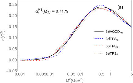
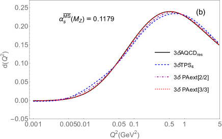
Figure 3: The same as in Figs. 2, but in 3$\delta$AQCD (instead of 2$\delta$AQCD). We note that the $3\delta$PAext[3/3] curve practically (visually) coincides with the resummed curve.

We present in Figs. 2(a) and 3(a) the results for $d(Q^{2})$ in 2$\delta$AQCD and 3$\delta$AQCD in the resummed form (6) and compare them to the truncated “perturbation” series in logarithmic derivatives in those models, i.e., AQCD analogs of the pQCD series Eq. (4b), as presented in Appendix A, Eqs. (25)-(26), with $\kappa=1$ and truncated at $\sim{\widetilde{\mathcal{A}}}_{N}$

$$d(Q^{2})_{\rm AQCD}^{[N]}={\mathcal{A}}(Q^{2})+{{\widetilde{d}}}_{1}\;{{{\widetilde{\mathcal{A}}}}}_{2}(Q^{2})+\ldots+{{\widetilde{d}}}_{N-1}\;{{{\widetilde{\mathcal{A}}}}}_{N}(Q^{2}),$$ (10)

where we denoted as earlier, for simplicity, ${\widetilde{d}}_{n}(\kappa=1)\equiv{\widetilde{d}}_{n}$. We note that formally, ${\widetilde{\mathcal{A}}}_{N}\sim a^{N}$ where $a$ is the underlying pQCD coupling. We can observe in Fig. 2(a), and to a lesser degree in 3(a), numerical indications that the truncated AQCD series (10) give us a divergent sequence when the truncation index $N$ increases (in the figures we have $4\leq N\leq 6$), i.e., we have no convergence to the resummed curves when $N$ increases.

On the other hand, in Figs. 2(b) and 3(b) we include the curves of the Padé-related approximants ${\cal G}_{d}^{[M/M]}(Q^{2})_{{\rm AQCD}}$ (denoted as ’PAext[M/M]’: ’extensions’ of (diagonal) Padé’s). The approximants were introduced in the framework of pQCD in dBGpt . They were later applied in QCD variants with holomorphic coupling (AQCD, i.e., free of Landau singularities) in Refs. dBG1 ; dBG2 ; dBG3 ; renmod ; they were applied there to the (spacelike) Adler function and to related QCD observables. These approximants are briefly explained here in Appendix A [Eqs. (27)-(28)]. These approximants are constructed only from the first $N=2M$ expansion coefficients ${\widetilde{d}}_{n}(\kappa)$ of $d(Q^{2})$ [i.e., from the coefficients ${\widetilde{d}}_{j}(\kappa)$, $0\leq j\leq(2M-1)$], they are entirely independent of the renormalisation scale parameter $\kappa$, and they formally approximate $d(Q^{2})$ up to the precision $\sim{\widetilde{\mathcal{A}}}_{2M+1}$, i.e., the difference $[d(Q^{2})-{\cal G}_{d}^{[M/M]}(Q^{2})_{{\rm AQCD}}]$ is $\sim{\widetilde{\mathcal{A}}}_{2M+1}$ (and this is formally $\sim a^{2M+1}$, where $a$ is the underlying pQCD coupling). We can see in Figs. 2(b) and 3(b) that these approximants converge fast toward the resummed value of $d(Q^{2})$, Eq. (6), when $N$($=2M$) increases. This is in stark contrast to the corresponding truncated series approximants (10) with $N=2M$, cf. Figs. 2(a) and 3(a).

IV Fits to the experimental data, in AQCD

The experimental data for inelastic BSR ${\overline{\Gamma}}_{1}^{\rm p-n}(Q^{2})$ have been obtained by various experiments CERN ; DESY ; SLAC ; JeffL1 ; JeffL2 ; JeffL3 ; JeffL4 ; JeffL5 , for the range $0<Q^{2}<5\ {\rm GeV}^{2}$. Our compilation of these data, for $0<Q^{2}\leq 4.739\ {\rm GeV}^{2}$, with statistical and systematic uncertainties, is presented in Figs. 2 of our previous work pPLB , and will be used here as well.

In this Section we will present the fit results with the approach Eq. (6) using the 2$\delta$AQCD and 3$\delta$AQCD couplings, and compare them with the same approach using pQCD coupling (in the P44 scheme with $c_{2}=9.$ and $c_{3}=20.$) that were obtained in our previous work pPLB .

We perform the fit where the above experimental values are fitted with the theoretical OPE expresssion Eq. (1) truncated either at $D=2$, or at $D=4$, and where the QCD canonical part $d(Q^{2})$ is evaluated with the renormalon-based resummation Eq. (6).

The fit consists of varying either the one fit parameter ${\bar{f}}_{2}$, or the two fit parameters ${\bar{f}}_{2}$ and $\mu_{6}$, cf. Eq. (1), such that the quantity

$$\chi^{2}(j_{\rm min};k)=\frac{1}{(j_{\rm max}-j_{\rm min}+1-N_{\rm p})}\sum_{j=j_{\rm min}}^{j_{\rm max}}\frac{\left[{\overline{\Gamma}}_{1}^{{\rm p-n},{\rm OPE}}(Q_{j}^{2})-{\overline{\Gamma}}_{1}^{{\rm p-n}}(Q_{j}^{2})_{\rm exp}\right]^{2}}{\sigma(Q_{j}^{2};k)^{2}}$$ (11)

is minimised. Here, $Q^{2}_{j}$ (where: $j=1,\ldots,j_{\rm max}$; $j_{\rm max}=77$) are the squared momentum scales at which the experimental data are available $(Q_{1}^{2}<Q_{2}^{2}<\cdots<Q_{77}^{2})$. Further, $N_{\rm p}$ is the number of fit parameters: $N_{\rm p}=1$ if $\mu_{6}=0$ and ${\bar{f}}_{2}$ is varied; $N_{\rm p}=2$ if both ${\bar{f}}_{2}$ and $\mu_{6}$ are varied. The index parameter $j_{\rm min}$ indicates a chosen minimal $Q^{2}_{\rm min}=Q^{2}_{j_{\rm min}}$ scale for which the experimental data are included in the fit; and $j_{\rm max}=77$ corresponds to the maximal fit scale, $Q^{2}_{\rm max}=Q_{77}^{2}=4.739\ {\rm GeV}^{2}$. Hence, the interval of scales included in the fit is: $Q^{2}_{\rm j_{\rm min}}\leq Q^{2}\leq 4.739\ {\rm GeV}^{2}$. The uncorrelated squared uncertainties $\sigma(Q_{j}^{2};k)^{2}$ at $Q_{j}^{2}$ in the expression (11) are in principle unknown. The statistical errors $\sigma_{\rm stat}(Q_{j}^{2})$ are expected to be largely uncorrelated, but the systematic errors $\sigma_{\rm sys}(Q_{j}^{2})$ may have significant, but unknown, correlations. Therefore, we follow here the method of unbiased estimate Deuretal2022 ; PDG2020 ; Schmell1995 . This method consists of the following. A fraction of $\sigma^{2}_{\rm sys}(Q_{j}^{2})$ is added to $\sigma^{2}_{\rm stat}(Q_{j}^{2})$

$$\sigma^{2}(Q_{j}^{2};k)=\sigma^{2}_{\rm stat}(Q_{j}^{2})+k\;\sigma^{2}_{\rm sys}(Q_{j}^{2}).$$ (12)

The obtained uncertainties $\sigma(Q_{j}^{2};k)$ are regarded as uncorrelated, and the mentioned fit parameters (only ${\bar{f}}_{2}$; or ${\bar{f}}_{2}$ and $\mu_{6}$) are extracted by minimisation of the above expression $\chi^{2}(j_{\rm min};k)$, Eq. (11), in the mentioned chosen interval of $Q^{2}$ values. This process is continued, by adjusting iteratively the parameter $k$ and minimising $\chi^{2}(j_{\rm min};k)$ until the value $\chi^{2}(j_{\rm min};k)=1$ is obtained. In practice, in this way we always obtain $0<k<0.5$. We note that the smaller the obtained value of $k$, the better is the fit.

The experimental uncorrelated uncertainty (exp.u.) of the obtained fit parameters (${\bar{f}}_{2}$; or ${\bar{f}}_{2}$ and $\mu_{6}$) is then obtained by the conventional methods as explained, e.g., in App. of Ref. Bo2011 , or App. D of ACT2023 . For completeness, we describe this method of obtaining ’exp.u.’ in Appendix B.

The experimental correlated uncertainty (exp.c.) is then obtained by simply shifting the central experimental values ${\overline{\Gamma}}_{1}^{{\rm p-n}}(Q_{j}^{2})_{\rm exp}$ in the expression (11) by the errors complementary to $\sigma(Q_{j}^{2};k)$ of Eq. (12), namely by $(1-\sqrt{k})\sigma_{\rm sys}(Q_{j}^{2})$, up and down, and conducting the minimisation of this new $\chi^{2}(j_{\rm min};k)$. The corresponding variation ’(exp.c.)’ of the extracted parameters is then the difference between such “shifted” extracted values and the central (“unshifted”) values.

Another question is how to choose the preferred value of $Q^{2}_{\rm min}$ ($=Q^{2}_{j_{\rm min}}$). The results of the fit can depend considerably on the choice of the value of $Q^{2}_{\rm min}$. In pQCD, the choice was $Q^{2}_{\rm min}=1.71\ {\rm GeV}^{2}$ in the fit with either two parameters (${\bar{f}}_{2}$, $\mu_{6}$) or one parameter (${\bar{f}}_{2}$), we refer for details to pPLB .

As mentioned, in the present resummation approach with AQCD couplings, Eq. (6), the employed variants are 2$\delta$AQCD 2dAQCD ; 2dAQCDb and 3$\delta$AQCD 3dAQCD ; 3dAQCDb , they are briefly described also here in Appendix A and were mentioned in Sec. III. The renormalisation schemes for 2$\delta$AQCD coupling are again taken to be the P44-schemes with the $c_{2}$ and $c_{3}$ beta-parameters varying in the range (9) as in pQCD; i.e., the central case will be again $c_{2}=9.$ and $c_{3}=20$. On the other hand, the 3$\delta$QCD coupling is related to the large volume lattice results BIMS1 ; BIMS2 and is thus in a fixed lattice-related scheme, the Lambert MiniMOM (LMM) P44-scheme MM1 ; MM2a ; MM2b ; MM3 ($c_{2}^{\rm LMM}=9.2980$ and $c_{3}^{\rm LMM}=71.4538$). As explained in Appendix A, in each of the two mentioned AQCD couplings, the parameters that fix the coupling are two: (a) the value of $\alpha_{s}^{\overline{\rm MS}}(M_{Z}^{2})$ that determines the ($N_{f}=3$) scale $\Lambda_{L}$ and thus determines the underlying $N_{f}=3$ pQCD coupling; (b) the scale (in GeV) of the lowest threshold mass $M_{1}=\sqrt{\sigma_{\rm min}}$ of the spectral (discontinuity) function $\rho(\sigma)={\rm Im}{\mathcal{A}}(-\sigma-i\epsilon)$. The threshold scale $M_{1}$ is expected to be of the order of the lowest hadronic scale, $M_{1}\sim m_{\pi}\approx 0.150$ GeV. So, for the central case, we fix the threshold scale to the value $M_{1}=0.150$ GeV and take $\alpha_{s}^{\overline{\rm MS}}(M_{Z}^{2})=0.1179$.

The fitting procedure gives for the 2$\delta$AQCD coupling for the two-parameter fit the values $k=0.1330$ and

$${\bar{f}}_{2}^{(2\delta)} = -0.0046^{+0.0145}_{-0.0106}(c_{2})^{+0.0080}_{-0.0145}(c_{3})^{+0.0487}_{-0.0464}(\alpha_{s})\pm 0.0034(d_{4})^{-0.0764}_{+0.0554}(M_{1})$$ (13a)

$${}^{+0.0373}_{-0.0231}(Q^{2}_{\rm min})\pm 0.0232({\rm exp.u.})\pm 0.1317({\rm exp.c.}),$$

$$\mu_{6}^{(2\delta)} = +0.0015\mp 0.0001(c_{2})^{+0.0007}_{-0.0005}(c_{3})^{-0.0027}_{+0.0024}(\alpha_{s})\mp 0.0005(d_{4})^{-0.0001}_{-0.0002}(M_{1})$$ (13b)

$${}^{-0.0073}_{+0.0034}(Q^{2}_{\rm min})\pm 0.0031({\rm exp.u.})\mp 0.0149({\rm exp.c.})\;[{\rm GeV}^{4}].$$

For the one-parameter fit with $2\delta$AQCD we obtain the values $k=0.1283$ and

$${\bar{f}}_{2}^{(2\delta)} = +0.0066^{+0.0136}_{-0.0095}(c_{2})^{+0.0135}_{-0.0183}(c_{3})^{+0.0288}_{-0.0281}(\alpha_{s})^{-0.0002}_{+0.0003}(d_{4})^{-0.0769}_{+0.0542}(M_{1})$$ (14)

$${}^{-0.0066}_{+0.0050}(Q^{2}_{\rm min})\pm 0.0038({\rm exp.u.})\pm 0.0208({\rm exp.c.}).$$

For the 3$\delta$AQCD coupling for the two-parameter fit we obtain the values $k=0.1613$ and

$${\bar{f}}_{2}^{(3\delta)} = -0.2531^{+0.0244}_{-0.0238}(\alpha_{s})^{-0.0014}_{+0.0013}(d_{4})^{+0.0766}_{-0.0813}(M_{1})$$ (15a)

$${}^{+0.0210}_{-0.0128}(Q^{2}_{\rm min})\pm 0.0244({\rm exp.u.})\pm 0.1203({\rm exp.c.}),$$

$$\mu_{6}^{(3\delta)} = +0.0013^{-0.0017}_{+0.0016}(\alpha_{s})\pm 0.0002(d_{4})^{-0.0039}_{+0.0046}(M_{1})$$ (15b)

$${}^{-0.0037}_{+0.0019}(Q^{2}_{\rm min})\pm 0.0032({\rm exp.u.})\mp 0.0132({\rm exp.c.})\;[{\rm GeV}^{4}].$$

For the one-parameter fit with $3\delta$AQCD we obtain the values $k=0.1553$ and

$${\bar{f}}_{2}^{(3\delta)} = -0.2430^{+0.0113}_{-0.0111}(\alpha_{s})^{+0.0001}_{-0.0001}(d_{4})^{+0.0472}_{-0.0455}(M_{1})$$ (16)

$${}^{-0.0081}_{+0.0022}(Q^{2}_{\rm min})\pm 0.0042({\rm exp.u.})\pm 0.0203({\rm exp.c.}).$$

The parameter ${\bar{f}}_{2}$ that appears in the $D=2$ OPE term Eq. (1) is dimensionless, but the $D=4$ OPE parameter $\mu_{6}$ is in units of ${\rm GeV}^{4}$.

As mentioned above, for the 3$\delta$AQCD case we cannot present scheme uncertainties (’$c_{2}$’) and (’$c_{3}$’) because the construction of the 3$\delta$AQCD coupling is tied to the lattice (L)MM scheme. In the results (13)-(14), the (theoretical) uncertainties at ’$(c_{2})$’ and ’$(c_{3})$’ originate from the renormalisation scheme variation, Eq. (9). The uncertainty at ’$(\alpha_{s})$’ in all the above results originates from the world average $\alpha_{s}$-uncertainty $\alpha_{s}^{\overline{\rm MS}}(M_{Z}^{2})=0.1179\pm 0.0009$ PDG2023 . The (theoretical) uncertainty at (’$d_{4}$’) comes from the mentioned variation $d_{4}^{\overline{\rm MS}}\approx 1557.4\pm 32.8$. The (experimental) uncertaintites (exp.u.) and (exp.c) were explained earlier in this Section.

In comparison to the pQCD case pPLB , we now have no (’ren’) uncertainties coming from the renormalon ambiguity, because no regularisation is needed in the resummation (6). However, the somewhat analogous (theoretical) uncertainty is the (’$M_{1}$’) uncertainty in Eqs. (13)-(14) and (15)-(16), which comes by varying the mentioned threshold scale $M_{1}$ of the spectral function $\rho(\sigma)$ of the AQCD coupling; we performed the following variation of this scale: $M_{1}=0.150^{+0.100}_{-0.050}$ GeV.

Furthermore, the uncertainty (’$Q^{2}_{\rm min}$’) comes now from the following variation, in the 2$\delta$AQCD case:

$$(Q^{2}_{\rm min})^{(2\delta)}=0.592^{+0.198}_{-0.122}\;{\rm GeV}^{2},$$ (17)

which is the same in the two-parameter and one-parameter fit. And in the 3$\delta$AQCD case the variation is

$$(Q^{2}_{\rm min})^{(3\delta),{\rm 2p}} = 0.592^{+0.106}_{-0.096}\;{\rm GeV}^{2},$$ (18a)

$$(Q^{2}_{\rm min})^{(3\delta),{\rm 1p}} = 0.592^{+0.198}_{-0.096}\;{\rm GeV}^{2},$$ (18b)

where in the superscripts ’2p’ and ’1p’ mean two-parameter and one-parameter fit, respectively. The central values for $Q^{2}_{\rm min}$, in Eqs. (17)-(18), were obtained in the following way. For each possible $Q^{2}_{\rm min}=Q^{2}_{j}$ ($1<j<77$), the fits were performed and the corresponding value of the $\sigma^{2}$-parameter $k$, Eq. (12), was obtained. The results are presented in Figs. 4. The preferred values of $Q^{2}_{\rm min}$ should not be too close to $Q^{2}_{\rm max}=Q_{77}=4.739\ {\rm GeV}^{2}$, in order to have a reasonably wide $Q^{2}$-interval for the fitted experimental values. Since the minimal $k$ represents the best fit, we choose such $Q^{2}_{\rm min}$ where the approximately minimal value of $k$ is obtained. This gives the central values of $Q^{2}_{\rm min}$ given above. The variation range of $Q^{2}_{\rm min}$, as given for each case in Eqs. (17)-(18), was then obtained by requiring that beyond the above ranges a relatively abrupt change (increase) in the value of $k$ occurs.

We can compare the obtained results Eqs. (13) and (15) of the two-parameter fits with the analogous two-parameter fit with pQCD coupling obtained in pPLB

$${\bar{f}}_{2}^{\rm(pQCD)} = -0.160^{-0.007}_{+0.025}(c_{2})^{+0.054}_{-0.039}(c_{3})^{+0.044}_{-0.041}(\alpha_{s})^{-0.012}_{+0.016}(d_{4})\mp 0.043({\rm ren})$$ (19a)

$${}^{+0.016}_{+0.119}(Q^{2}_{\rm min})\pm 0.160({\rm exp.u.})\pm 0.297({\rm exp.c.}),$$

$$\mu_{6}^{\rm(pQCD)} = +0.022^{+0.003}_{-0.008}(c_{2})^{-0.013}_{+0.004}(c_{3})^{-0.010}_{+0.008}(\alpha_{s})^{+0.002}_{-0.003}(d_{4})\mp 0.010({\rm ren})$$ (19b)

$${}^{-0.006}_{-0.053}(Q^{2}_{\rm min})\pm 0.062({\rm exp.u.})\mp 0.059({\rm exp.c.})\;[{\rm GeV}^{4}],$$

and where we had $k=0.1621$ and $Q^{2}_{\rm min}=1.71^{+0.205}_{-0.27}\ {\rm GeV}^{2}$.

Further, the results Eq. (14) and (16) of the one-parameter fits can be compared with the analogous one-parameter fit with pQCD coupling obtained in pPLB

$${\bar{f}}_{2}^{\rm(pQCD)} = -0.107^{-0.001}_{+0.007}(c_{2})^{+0.022}_{-0.029}(c_{3})\pm 0.020(\alpha_{s})\mp 0.009(d_{4})\mp 0.067({\rm ren})$$ (20)

$${}^{+0.012}_{-0.029}(Q^{2}_{\rm min})\pm 0.033({\rm exp.u.})\pm 0.154({\rm exp.c.}),$$

and where we had $k=0.1487$ and $Q^{2}_{\rm min}=1.71^{+0.39}_{-0.27}\ {\rm GeV}^{2}$.

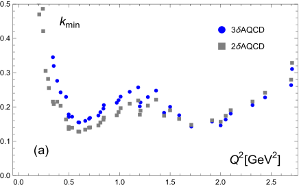
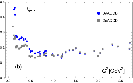
Figure 4: The values of the $\sigma^{2}$-parameter $k$, Eq. (12), for various $Q^{2}=Q^{2}_{\rm min}$ for the 2$\delta$ and 3$\delta$AQCD coupling: (a) when one-parameter fit is performed; (b) when two-parameter fit is performed.

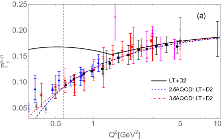
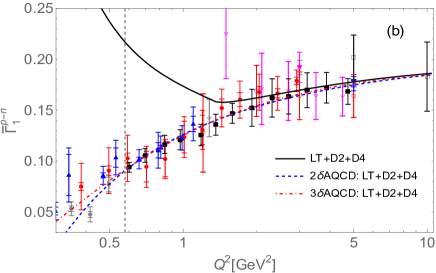
Figure 5: The fitted curves for the BSR ${\overline{\Gamma}}_{1}^{\rm p-n}(Q^{2})$: (a) for the one-parameter fits; (b) for the two-parameter fits. The couplings used are 2$\delta$AQCD and 3$\delta$AQCD. Experimental data, and the corresponding pQCD fit (here as solid line; $Q^{2}_{\rm min}=1.71\ {\rm GeV}^{2}$), are included for comparison. See the text for details. The vertical line indicates the value of the left end of the fit interval for the AQCD curves, $Q^{2}_{\rm min}=0.592\ {\rm GeV}^{2}$.

In Figs. 5(a), (b), we present the resulting fitting curves ${\overline{\Gamma}}_{1}^{\rm p-n}(Q^{2};{\bar{f}}_{2})$ and ${\overline{\Gamma}}_{1}^{\rm p-n}(Q^{2};{\bar{f}}_{2},\mu_{6})$ for 2$\delta$AQCD and 3$\delta$AQCD, using the corresponding central values of parameters of Eqs. (13)-(16). The corresponding central values for the other parameters were used (scheme, $\alpha_{s}^{\overline{\rm MS}}(M_{Z}^{2})$, $M_{1}$, $d_{4}$). For comparison, the experimental data, and the corresponding pQCD fit (with $Q^{2}_{\rm min}=1.71\ {\rm GeV}^{2}$), are included in the Figures.

V Discussion of the results, and conclusions

In this work, we performed various analyses of the inelastic Bjorken polarised sum rule (BSR) ${\overline{\Gamma}}_{1}^{{\rm p-n}}(Q^{2})$. The theoretical basis was the OPE (1) truncated at the dimension $D=4$ or $D=2$ term. The canonical leading-twist QCD contribution $d(Q^{2})$ was evaluated by a renormalon-based resummation, Eq. (6), using two types of the holomorphic (AQCD) running couplings, $\alpha_{s}(Q^{{}^{\prime}2})/\pi\mapsto{\mathcal{A}}(Q^{{}^{\prime}2})$, that are free of Landau singularities: 2$\delta$AQCD and 3$\delta$AQCD couplings ${\mathcal{A}}(Q^{{}^{\prime}2})$. This work can be regarded as a continuation of our previous work pPLB where the analyses were performed using the same kind of resummation but with perturbative QCD (pQCD) couplings $\alpha_{s}(Q^{{}^{\prime}2})/\pi\equiv a(Q^{{}^{\prime}2})$ that do have Landau singularities and thus a regularisation was needed, cf. Eq. (5). These resummations, Eqs. (5)-(6), are completely invariant under the renormalisation scale variation. The obtained theoretical (truncated OPE) expression Eq. (1) was then fitted to the available data points for BSR.

In general, the experimental data have too high uncertainties for the extraction of the preferred value of $\alpha_{s}^{\overline{\rm MS}}(M_{Z}^{2})$, especially when we include the $D=4$ term in the OPE. Therefore, we fixed this value to $\alpha_{s}^{\overline{\rm MS}}(M_{Z}^{2})=0.1179$, the central world average value PDG2023 . The resulting extracted values of the OPE fit parameters ${\bar{f}}_{2}$ and $\mu_{6}$ are given for the 2$\delta$AQCD case in Eqs. (13)-(14), and for the 3$\delta$AQCD case in Eqs. (15)-(16), and can be compared with values for the pQCD case obtained in Ref. pPLB [cf. Eqs. (19)-(20) here]. The various experimental uncertainties of the extracted values, Eqs. (13)-(16), are represented by the last three terms there: (’$Q^{2}_{\rm min}$’), (exp.u.) and (exp.c.). We see that the experimental uncertainties are in general the dominant ones, especially the correlated uncertainty (exp.c.). The various theoretical uncertainties are in general smaller than the experimental ones, sometimes with the exception of the (’$M_{1}$’) uncertainty in AQCD cases, i.e., the uncertainty due to the variation of the spectral function of the holomorphic coupling at low scales $M_{1}$. Furthermore, when compared to the pQCD case Eqs. (19)-(20), we see that the use of AQCD couplings in general reduces the experimental uncertainties of the extracted values by large factors in comparison to the pQCD case, in some cases by one order of magnitude. Additionally, the use of AQCD couplings in the two-parameter fit gives very suppressed values of the $D=4$ parameter $\mu_{6}$, thus largely reducing the need to include the $D=4$ OPE term.

The (resummed) AQCD results have yet another attractive feature when compared to the (resummed) pQCD results: the preferred fit interval is considerably wider, $0.592\ {\rm GeV}^{2}\leq Q^{2}\leq 4.739\ {\rm GeV}^{2}$, than in the pQCD case where it was restricted to $1.710\ {\rm GeV}^{2}\leq Q^{2}\leq 4.739\ {\rm GeV}^{2}$. One reason for this is that the pQCD running coupling $a(Q^{{}^{\prime}2})$ has Landau cut singularities at low positive values $Q^{{}^{\prime}2}\lesssim 1\ {\rm GeV}^{2}$, while the AQCD couplings ${\mathcal{A}}(Q^{{}^{\prime}2})$ are free of such singularities.

If we apply in the pQCD approach, instead of the resummation (5) in the canonical QCD part $d(Q^{2})$, a simple truncated power series in $a(\mu^{2})$ (TPS), the results further change significantly. For example, the TPS approach in $\overline{\rm MS}$ scheme and with $\alpha_{s}^{\overline{\rm MS}}(M_{Z}^{2})=0.1179$, leads to significant renormalisation scale dependence, and the truncation index ($N_{\rm tr}$) dependence. If we choose $\mu^{2}=Q^{2}$, the two-parameter fit results are strongly $N_{\rm tr}$-dependent, at $N_{\rm tr}=8$ we obtain small $\chi^{2}=0.891$ but the values ${\bar{f}}_{2}\approx-0.44$ and $\mu_{6}=0.43\ {\rm GeV}^{4}$ are large and lead to significant cancellation effects between $D=2$ and $D=4$ BSR terms in the range $2\ {\rm GeV}^{2}<Q^{2}<3\ {\rm GeV}^{2}$. On the other hand, for $N_{\rm tr}\geq 10$ we obtain very large $\chi^{2}>4$. The one-parameter fit results give for all $N_{\rm tr}\geq 3$ the values $\chi^{2}>1$, and the values of $\chi^{2}$ increase when $N_{\rm tr}$ increases. These results strongly suggest that the TPS approach in pQCD is less reliable than the (renormalon-based) pQCD resummation approach Eq. (5).

On the other hand, in the holomorphic QCD (i.e., AQCD) the Padé-related approximants ${\cal G}_{d}^{[M/M]}(Q^{2})$, which are constructed only from the first $2M$ expansion coefficients ${\widetilde{d}}_{n}(\kappa)$ of $d(Q^{2})$, are completely independent of the renormalisation scale parameter $\kappa$ and converge rapidly to the fully resummed values of $d(Q^{2})$ of Eq. (6) for all $Q^{2}$ when $M$ increases. These approximants in general do not work well when pQCD coupling is used, due to the Landau singularities of such a coupling.

Our results suggest that for an improved theoretical description of low-energy spacelike observables such as BSR it is important: (a) to perform the fit with resummation of $d(Q^{2})$ according to Eqs. (5) or (6) instead of using truncated expressions; (b) to use, in the resummation, for the running coupling, instead of the pQCD coupling $a(Q^{{}^{\prime}2})$, a holomorphic coupling ${\mathcal{A}}(Q^{{}^{\prime}2})$, i.e., a coupling that is practically equal to the (underlying) pQCD coupling $a(Q^{{}^{\prime}2})$ at high scales $Q^{{}^{\prime}2}>1\ {\rm GeV}^{2}$ and is regulated in the low-scale regime $Q^{{}^{\prime}2}\lesssim 1\ {\rm GeV}^{2}$ such that it has no Landau singularities there.

In our work we did not consider models for inelastic BSR ${\overline{\Gamma}}_{1}^{{\rm p-n}}(Q^{2})$ at very low $Q^{2}<1\ {\rm GeV}^{2}$, e.g., expansions JeffL2 motivated on chiral perturbation theory or the light-front holographic QCD (LFH) LFH1 ; LFHBSR . In one of our previous works ACKS we included such low-$Q^{2}$ models in the analysis. In the present work, the main emphasis was to construct a renormalon-based extension (to all orders) of the expansion of the canonical BSR part $d(Q^{2})$, and to resum it with the approach of characteristic function in the framework of AQCD variants, Eq. (6). With these results, the corresponding OPE was fitted to the experimental data.

We performed numerical analyses (fits) with mathematica software. The mathematica programs that were constructed and used in the numerical analyses in this work are available on the web page www , and they include the experimental data.

Appendix A 2$\delta$AQCD and 3$\delta$AQCD

Here we summarise the construction of 2$\delta$AQCD 2dAQCD ; 2dAQCDb and 3$\delta$AQCD 3dAQCD ; 3dAQCDb , i.e., versions ${\mathcal{A}}(Q^{2})$ of the QCD coupling that have no Landau singularities and practically coincide at high $Q^{2}>1\ {\rm GeV}^{2}$ with the underlying pQCD coupling $a(Q^{2})$ running in a P44-renormalisation scheme, Eqs. Eqs. (32)-(35) of pPLB . At low $Q^{2}\lesssim 1\ {\rm GeV}^{2}$, the coupling ${\mathcal{A}}(Q^{2})$ is required to fulfill certain additional conditions.

The starting point is the pQCD coupling $a(Q^{2})$ in a certain renormalisation scheme, for convenience the P44-scheme with chosen values of the scheme parameters $c_{2}$ and $c_{3}$, cf. Eqs. Eqs. (32)-(35) of pPLB . The resulting underlying ($N_{f}=3$) pQCD coupling $a(Q^{2})$ is given in terms of the Lambert function, cf. Eq. (34) of pPLB , it is given in terms of the Lambert function $W_{\pm 1}(z)$ (which is very convenient in practical evaluations), and it is an explicit function of any complex $Q^{2}$. This coupling $a(Q^{2})$ has discontinuity (cut) along the real axis; this discontinuity is usually called the spectral function of the coupling

$$\rho^{\rm(pt)}(\sigma)\equiv{\rm Im}\;a(-\sigma-i\epsilon),$$ (21)

which is thus again written in terms of the Lambert function $W_{\pm 1}(z)$ (and thus easily evaluated in practice). Since the coupling has Landau singularities, the spectral function is nonzero not just for $\sigma>0$ (i.e., $Q^{2}=-\sigma<0$), but also at some lower negative values $-\Lambda^{2}\leq\sigma\leq 0$) (i.e., $0\leq Q^{2}=-\sigma\leq\Lambda^{2}$) where usually $\Lambda^{2}\sim 0.1\ {\rm GeV}^{2}$.

The holomorphic coupling ${\mathcal{A}}(Q^{2})$ is then required to have the spectral function $\rho_{{\mathcal{A}}}(\sigma)\equiv{\rm Im}{\mathcal{A}}(-\sigma-i\epsilon)$ which coincides with the above spectral function $\rho^{\rm(pt)}(\sigma)$ for sufficiently large $\sigma>M_{0}^{2}$ ($>0$); for $0<\sigma<M_{0}^{2}$ deviations from $\rho^{\rm(pt)}(\sigma)$ are expected; and for $\sigma<0$ we require that $\rho_{{\mathcal{A}}}(\sigma)=0$ (i.e., that there are no Landau singularities). In the range $0<\sigma<M_{0}^{2}$ where $\rho_{{\mathcal{A}}}(\sigma)$ is not known, we parametrise it by a linear combination of $n$ Dirac delta functions [which corresponds to near-diagonal Padé expression contribution in ${\mathcal{A}}(Q^{2})$, see later]

$$\rho_{{\mathcal{A}}}^{(n\delta)}(\sigma)=\pi\sum_{j=1}^{n}{\cal F}_{j}\;\delta(\sigma-M_{j}^{2})+\Theta(\sigma-M_{0}^{2})\rho^{\rm(pt)}(\sigma)\ .$$ (22)

By notational convention, we have ($0<$) $M_{1}^{2}<M_{2}^{2}<\cdots<M_{n}^{2}<M_{0}^{2}$, and $M_{1}^{2}=M^{2}_{\rm thr}$ is interpreted as the threshold scale of the spectral function $\rho_{{\mathcal{A}}}$; it is expected to be in the range of the lowest hadronic scales, i.e., $M_{1}^{2}\sim m_{\pi}^{2}$ ($\sim 10^{-2}\ {\rm GeV}^{2}$). On the other hand, $M_{0}^{2}$ ($\sim 1\ {\rm GeV}^{2}$) can be interpreted as the pQCD-onset scale. Using the Cauchy theorem, we then obtain from the spectral function (22) the running coupling ${\mathcal{A}}(Q^{2})$

$${\mathcal{A}}^{(n\delta)}(Q^{2})\left(\equiv\frac{1}{\pi}\int_{0}^{\infty}d\sigma\frac{\rho_{{\mathcal{A}}}(\sigma)}{(\sigma+Q^{2})}\right) = \sum_{j=1}^{n}\frac{{\cal F}_{j}}{(Q^{2}+M_{j}^{2})}+\frac{1}{\pi}\int_{M_{0}^{2}}^{\infty}d\sigma\frac{\rho_{1}^{\rm(pt)}(\sigma)}{(Q^{2}+\sigma)}\ .$$ (23)

The obtained coupling has altogether $(2n+1)$ parameters: ${\cal F}_{j}$ and $M_{j}^{2}$ ($j=1,\ldots,n$) and $M_{0}^{2}$. They are then fixed by various conditions. The condition that the coupling should practically coincide with the underlying pQCD coupling $a(Q^{2})$ at sufficiently high $|Q^{2}|>1\ {\rm GeV}^{2}$ is implemented in our approch in the following specific way:

$${\mathcal{A}}(Q^{2})-a(Q^{2})\sim\left(\frac{\Lambda_{L}^{2}}{Q^{2}}\right)^{5}\qquad(|Q^{2}|>\Lambda_{L}^{2}).$$ (24)

In general, the above difference would be $\sim(\Lambda_{L}^{2}/Q^{2})^{1}$; therefore, the condition (24) represents four conditions.

In the 2$\delta$AQCD, we have $n=2$ and thus five parameters. We can choose a value of the threshold scale $M_{1}^{2}$ as an input, and then the four remaining parameters are fixed by the conditions (24). We note that in the 2$\delta$AQCD, the underlying pQCD coupling can be in any chosen P44-scheme (i.e., with any chosen values of $c_{2}$ and $c_{3}$).

In 3$\delta$AQCD, we have $n=3$ and thus seven parameters. The conditions (24) represent four conditions. Two additional conditions are obtained if we require that ${\mathcal{A}}(Q^{2})^{(3\delta)}$ behaves at low $Q^{2}$ as a specific product of the Landau gauge gluon and ghost dressing functions whose behaviour at low positive $Q^{2}$ was obtained by large volume lattice calculations BIMS1 ; BIMS2 . For details we refer to 3dAQCD ; 3dAQCDb . These two conditions, are that ${\mathcal{A}}(Q^{2})$ at positive $Q^{2}$ achieves the local maximum at $Q^{2}\approx 0.135\ {\rm GeV}^{2}$ and that it behaves as ${\mathcal{A}}(Q^{2})\sim Q^{2}$ ($\to 0$) at very low $Q^{2}$ ($0<Q^{2}\lesssim 0.1\ {\rm GeV}^{2}$). This gives us additional two conditions, adding up to altogether six conditions. The seventh condition, necessary to fix all the seven parameters, is again the choice of the threshold scale $M_{1}^{2}$ ($\sim m_{\pi}^{2}$).

In Tables 1 and 2 we present the values of the parameters of the 2$\delta$AQCD and 3$\delta$AQCD coupling for the relevant cases used in this work.

Table 1: Values of the parameters of the 2$\delta$AQCD coupling used in this work; the first entry is for the central case: P44-scheme with $c_{2}=9.$ and $c_{3}=20.$; $M_{1}=0.150$ GeV; $\alpha_{s}^{\overline{\rm MS}}(M_{Z}^{2})=0.1179$; the other entries are for the case when one of these parameters changes. The dimensionless parameters are $s_{j}=M_{j}^{2}/\Lambda_{L}^{2}$ and $f_{j}={\cal F}_{j}/\Lambda_{L}^{2}$. $\Lambda_{L}$ is the Lambert scale of the underlying pQCD coupling, fixed by the condition $\alpha_{s}^{\overline{\rm MS}}(M_{Z}^{2})=0.1179$.

case	$s_{1}$	$s_{2}$	$f_{1}$	$f_{2}$	$s_{0}$	$\Lambda_{{\rm L}}$ [GeV]
central	0.47584	68.8281	1.71541	0.94206	95.8788	0.21745
$c_{2}=11.$, $c_{3}=20.$	0.47581	80.6865	1.93086	1.07273	112.47	0.21745
$c_{2}=7.6$, $c_{3}=20.$	0.47583	61.3845	1.57632	0.85810	85.4648	0.21745
$c_{2}=9.$, $c_{3}=35.$	0.77003	121.627	2.92848	1.62931	169.534	0.17094
$c_{2}=9.$, $c_{3}=5.$	0.22581	28.9299	0.75915	0.40791	40.2527	0.31566
$M_{1}=0.250$ GeV	1.32175	74.2430	1.77216	0.98111	103.039	0.21745
$M_{1}=0.100$ GeV	0.21148	67.1287	1.69729	0.92969	93.6321	0.21745
$\alpha_{s}^{\overline{\rm MS}}(M_{Z}^{2})=0.1188$	0.43937	68.5939	1.71292	0.94036	95.5691	0.22630
$\alpha_{s}^{\overline{\rm MS}}(M_{Z}^{2})=0.1170$	0.51606	69.0864	1.7181	0.94393	96.2202	0.20881

Table 2: Values of the parameters of the 3$\delta$AQCD coupling used in this work; the first entry is for the central case: P44 LMM scheme (i.e., $c_{2}=9.29703$ and $c_{3}=71.4538$); $M_{1}=0.150$ GeV; $\alpha_{s}^{\overline{\rm MS}}(M_{Z}^{2})=0.1179$; the other entries are for the case when $M_{1}$ changes, or $\alpha_{s}^{\overline{\rm MS}}(M_{Z}^{2})$ changes. The dimensionless parameters are $s_{j}=M_{j}^{2}/\Lambda_{L}^{2}$ and $f_{j}={\cal F}_{j}/\Lambda_{L}^{2}$. $\Lambda_{L}$ is the Lambert scale of the underlying pQCD coupling.

case	$s_{1}$	$s_{2}$	$s_{3}$	$f_{1}$	$f_{2}$	$f_{3}$	$s_{0}$	$\Lambda_{{\rm L}}$ [GeV]
central	1.79371	42.9853	607.164	-0.586232	10.6669	6.06743	827.469	0.11200
$M_{1}=0.250$ GeV	4.98252	16.7070	470.372	-4.37049	13.2756	5.23222	647.009	0.11200
$M_{1}=0.100$ GeV	0.79720	88.0403	862.126	-0.16976	12.2415	7.52131	1163.66	0.11200
$\alpha_{s}^{\overline{\rm MS}}(M_{Z}^{2})=0.1188$	1.65625	40.3300	589.951	-0.562248	10.5011	5.9629	804.698	0.11655
$\alpha_{s}^{\overline{\rm MS}}(M_{Z}^{2})=0.1170$	1.94533	45.8556	625.783	-0.61228	10.8448	6.17983	852.102	0.10755

In Fig. 6 we present the behaviour of various ($N_{f}=3$) running couplings: pQCD coupling $a(Q^{2})_{\overline{\rm MS}}$ in the 5-loop $\overline{\rm MS}$ scheme; pQCD coupling $a(Q^{2})$ in the P44-scheme with $c_{2}=9.$ and $c_{3}=20.$; 2$\delta$AQCD coupling ${\mathcal{A}}(Q^{2})^{(2\delta)}$ (in the mentioned P44 scheme with $c_{2}=9.$ and $c_{3}=20.$); and 3$\delta$AQCD coupling ${\mathcal{A}}(Q^{2})^{(3\delta)}$ in the P44 LMM scheme ($c_{2}=9.29703$ and $c_{3}=71.4538$).

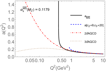
Figure 6: Various ($N_{f}=3$) running couplings: pQCD coupling $a(Q^{2})_{\overline{\rm MS}}$ in the 5-loop $\overline{\rm MS}$ scheme; 2$\delta$AQCD coupling ${\mathcal{A}}(Q^{2})^{(2\delta)}$ and its underlying pQCD coupling $a(Q^{2})$, both in the P44 scheme with $c_{2}=9.$ and $c_{3}=20.$; 3$\delta$AQCD coupling ${\mathcal{A}}(Q^{2})^{(3\delta)}$, in the (lattice-related) P44 LMM scheme.

The coupling $a(Q^{2})$ has Landau cut for $Q^{2}<0.87\ {\rm GeV}^{2}$, and $a(Q^{2})_{\overline{\rm MS}}$ for $Q^{2}<0.40\ {\rm GeV}^{2}$. We note that at the corresponding branching points $a(Q^{2})$ is finite and $a(Q^{2})_{\overline{\rm MS}}$ is infinite. The AQCD couplings have neither Landau cuts nor infinities. The coupling ${\mathcal{A}}(Q^{2})^{(2\delta)}$ grows at decreasing $Q^{2}$ and reaches a large, but finite value ${\mathcal{A}}(0)^{(2\delta)}=3.6970$ at $Q^{2}=0$. All couplings correspond to the reference value $\alpha_{s}^{\overline{\rm MS}}(M_{Z}^{2};N_{f}=5)=0.1179$, and the AQCD couplings have the spectral threshold scale $M_{1}=0.150$ GeV.

Further, in Figs. 7(a),(b), we present separately the 2$\delta$AQCD and 3$\delta$AQCD running couplings; for comparison, we include the corresponding underlying pQCD couplings $a(Q^{2})$.

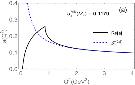
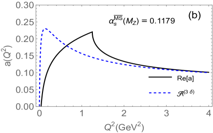
Figure 7: The AQCD running coupling ${\mathcal{A}}(Q^{2})$ and their corresponding underlying pQCD coupling $a(Q^{2})$: (a) for 2$\delta$AQCD (in the scheme P44 with $c_{2}=9.$ and $c_{3}=20.$); (b) for 3$\delta$AQCD (in the P44 LMM scheme). The coupling $a(Q^{2})$ has Landau cut at $0\leq Q^{2}<0.87\ {\rm GeV}^{2}$ in the 2$\delta$ case, and at $0\leq Q^{2}<1.25\ {\rm GeV}^{2}$ in the 3$\delta$ case. Both these couplings $a(Q^{2})$ become complex on the Landau cut. Therefore, real part ${\rm Re}\ a(Q^{2})$ was presented in those intervals.

The expansions in AQCD are made in a completely analogous way as in pQCD, Eq. (4b), i.e., in terms of the logarithmic derivatives ${\widetilde{\mathcal{A}}}_{n}$ that are the AQCD analogs of the ${\widetilde{a}}_{n}$ logarithmic derivatives of pQCD coupling [cf. Eq. (3)]

$${{\widetilde{\mathcal{A}}}}_{n}(\mu^{2})\equiv\frac{(-1)^{n-1}}{(n-1)!\beta_{0}^{n-1}}\left(\frac{d}{d\ln\mu^{2}}\right)^{n-1}{\mathcal{A}}(\mu^{2})\qquad(n=1,2,\ldots).$$ (25)

$$d(Q^{2})={\mathcal{A}}(\kappa Q^{2})+{{\widetilde{d}}}_{1}(\kappa)\;{{{\widetilde{\mathcal{A}}}}}_{2}(\kappa Q^{2})+\ldots+{{\widetilde{d}}}_{n}(\kappa)\;{{{\widetilde{\mathcal{A}}}}}_{n+1}(\kappa Q^{2})+\ldots,$$ (26)

This expansion in AQCD was introduced in CV , and it has the form completely analogous to the pQCD expansion in logarithmic derivatives ${\widetilde{a}}_{n}$ Eq. (4b).^, Another, more efficient, sequence of approximants are specific type of approximants, ${\cal G}^{[M/M]}_{d}(Q^{2})$, which are related to the diagonal Padé approximants, and are constructed only on the basis of the knowledge of the first $2M$ coefficients of the series in ${\widetilde{a}}_{n}$ in pQCD, or equivalently of the series (26) in AQCD: ${\widetilde{d}}_{j}(\kappa)$ ($j=0,1,\ldots,2M-1$). The approximants ${\cal G}^{[M/M]}_{d}(Q^{2})$ were proposed in dBGpt in the context of pQCD, and were later applied in variants of AQCD in dBG1 ; dBG2 ; dBG3 ; renmod to the (spacelike) Adler function and to related QCD observables. They are completely independent of the renormalisation scale parameter $\kappa$. These approximants have in AQCD the form

$${\cal G}^{[M/M]}_{d}(Q^{2})_{{\rm AQCD}}=\sum_{k=1}^{M}{\widetilde{\alpha}}_{j}{\mathcal{A}}(\kappa_{j}Q^{2}),$$ (27)

and fulfill the approximant precision relation

$$d(Q^{2})-{\cal G}^{[M/M]}_{d}(Q^{2})_{{\rm AQCD}}={\cal O}({\widetilde{\mathcal{A}}}_{2M+1})={\cal O}(a^{2M+1}).$$ (28)

In pQCD, the same expression (27) is valid, but with ${\mathcal{A}}(\kappa_{j}Q^{2})$ replaced by the pQCD coupling $a(\kappa_{j}Q^{2})$.

We note that the approximant (27) contains in total $2M$ parameters: ${\widetilde{\alpha}}_{j}$ and $\kappa_{j}$, which are determined by the first $2M$ expansion coefficients ${\widetilde{d}}_{n}(\kappa)$ ($n=0,1,\ldots,2M-1$). As noted in dBGpt , the application of these approximants in pQCD gives for spacelike QCD observables $d(Q^{2})$ in general relatively unstable results, especially when $M$ increases, and this is so because some of the $\kappa_{j}$ coefficients are very small and then $a(\kappa_{j}Q^{2})$ is on Landau cut singularities. This problem does not appear in QCD with holomorphic couplings (AQCD), as noted in dBG1 ; dBG2 ; dBG3 ; renmod , because ${\mathcal{A}}(\kappa_{j}Q^{2})$ coupling has no Landau singularities.

In Table 3 we present the values of the parameters $\kappa_{j}$ and ${\widetilde{\alpha}}_{j}$ of the approximants ${\cal G}^{[M/M]}_{d}(Q^{2})$ for canonical BSR $d(Q^{2})$, for $M=2$ and $M=3$, for 2$\delta$QCD (in the P44 scheme with $c_{2}=9.$ and $c_{3}=20.$) and for 3$\delta$AQCD (in the P44 LMM scheme, i.e., with $c_{2}=9.29703$ and $c_{3}=71.4538$).

Table 3: Values of the parameters ${\widetilde{\alpha}}_{j}$ and $\kappa_{j}$ of the (diagonal Padé-related) approximants ${\cal G}^{[M/M]}_{d}(Q^{2})$, for 2$\delta$AQCD and 3$\delta$AQCD (in their respective P44-schemes), for $M=2$ and $M=3$.

QCD variant	$M$	${\widetilde{\alpha}}_{1}$	${\widetilde{\alpha}}_{2}$	${\widetilde{\alpha}}_{3}$	$\kappa_{1}$	$\kappa_{2}$	$\kappa_{3}$
2$\delta$AQCD	2	-0.011789	1.011789	–	462.707872	0.222567	–
2$\delta$AQCD	3	-0.045853	0.013012	1.032841	20.911126	0.0033448	0.263115
3$\delta$AQCD	2	-0.044854	1.044854	–	13.47291	0.243514	–
3$\delta$AQCD	3	-0.095297	0.008018	1.087279	4.781674	0.006406	0.275173

Appendix B The experimental uncorrelated uncertainty of the extracted parameter values

We summarise here the formula for the uncorrelated experimental uncertainties for the two-parameter fit (${\bar{f}}_{2}$ and $\mu_{6}$) of the (inelastic) BSR. This is a special case of the approach given in App. of Ref. Bo2011 (and App. D of ACT2023 ).

The fit consist of minimising the expression $\chi^{2}$ Eq. (11), where the two OPE parameters $p_{1}={\bar{f}}_{2}$ and $p_{2}=\mu_{6}$ are varied. The corresponding variations of these two parameters, due to the experimental uncertainties $\sigma(Q^{2}_{j})$ at each point $Q^{2}_{j}$, are

$$\langle\delta p_{1}\delta p_{1}\rangle = (A^{-1})_{1,1},$$ (29a)

$$\langle\delta p_{2}\delta p_{2}\rangle = (A^{-1})_{2,2},$$ (29b)

where the $2\times 2$ matrix $A$ is

$$A_{\ell,m}=\sum_{j=j_{\rm min}}^{j_{\rm max}}\frac{\partial{\overline{\Gamma}}_{1}^{{\rm p-n}}(Q^{2}_{j})}{\partial p_{\ell}}\frac{\partial{\overline{\Gamma}}_{1}^{{\rm p-n}}(Q^{2}_{j})}{\partial p_{m}}\frac{1}{\sigma(Q^{2}_{j})^{2}}\qquad(\ell,m=1,2).$$ (30)

Then the (uncorrelated) experimental uncertainties of the extracted values of $p_{1}={\bar{f}}_{2}$ and of $p_{2}=\mu_{6}$ are

$$\delta{\bar{f}}_{2}({\rm exp.u.}) = \sqrt{\langle\delta p_{1}\delta p_{1}\rangle}=\sqrt{(A^{-1})_{1,1}},$$ (31a)

$$\delta\mu_{6}({\rm exp.u.}) = \sqrt{\langle\delta p_{2}\delta p_{2}\rangle}=\sqrt{(A^{-1})_{2,2}},$$ (31b)

In the case of the one-parameter fit (${\bar{f}}_{2}$), analogous formulas hold, $A$ is in such a case only a number ($1\times 1$ matrix).

References

- (1) C. Ayala, C. Castro-Arriaza and G. Cvetič, “Evaluation of Bjorken polarised sum rule with a renormalon-motivated approach,” Phys. Lett. B 848 (2024), 138386 [arXiv:2309.12539 [hep-ph]]
- (2) J. D. Bjorken, “Applications of the Chiral U(6) x (6) Algebra of Current Densities,” Phys. Rev. 148 (1966), 1467-1478
- (3) J. D. Bjorken, “Inelastic Scattering of Polarized Leptons from Polarized Nucleons,” Phys. Rev. D 1 (1970), 1376-1379
- (4) B. Adeva et al. [Spin Muon (SMC)], “The Spin dependent structure function of the proton from polarized deep inelastic muon scattering,” Phys. Lett. B 412 (1997), 414-424; D. Adams et al. [Spin Muon (SMC)], “Spin structure of the proton from polarized inclusive deep inelastic muon - proton scattering,” Phys. Rev. D 56 (1997), 5330-5358 [arXiv:hep-ex/9702005 [hep-ex]]; E. S. Ageev et al. [COMPASS], “Measurement of the spin structure of the deuteron in the DIS region,” Phys. Lett. B 612 (2005), 154-164 [arXiv:hep-ex/0501073 [hep-ex]]; V. Y. Alexakhin et al. [COMPASS], “The Deuteron Spin-dependent Structure Function and its First Moment,” Phys. Lett. B 647 (2007), 8-17 [arXiv:hep-ex/0609038 [hep-ex]]; M. G. Alekseev et al. [COMPASS], “The Spin-dependent Structure Function of the Proton and a Test of the Bjorken Sum Rule,” Phys. Lett. B 690 (2010), 466-472 [arXiv:1001.4654 [hep-ex]]; C. Adolph et al. [COMPASS], “The spin structure function of the proton and a test of the Bjorken sum rule,” Phys. Lett. B 753 (2016), 18-28 [arXiv:1503.08935 [hep-ex]]; C. Adolph et al. [COMPASS], “Final COMPASS results on the deuteron spin-dependent structure function and the Bjorken sum rule,” Phys. Lett. B 769 (2017), 34-41 [arXiv:1612.00620 [hep-ex]]; M. Aghasyan et al. [COMPASS], “Longitudinal double-spin asymmetry and spin-dependent structure function of the proton at small values of and ,” Phys. Lett. B 781 (2018), 464-472 [arXiv:1710.01014 [hep-ex]]
- (5) K. Ackerstaff et al. [HERMES], “Measurement of the neutron spin structure function with a polarized 3He internal target,” Phys. Lett. B 404 (1997), 383-389 [arXiv:hep-ex/9703005 [hep-ex]]; A. Airapetian et al. [HERMES], “Measurement of the proton spin structure function with a pure hydrogen target,” Phys. Lett. B 442 (1998), 484-492 [arXiv:hep-ex/9807015 [hep-ex]]
- (6) K. Abe et al. [E143], “Measurements of the proton and deuteron spin structure functions and ,” Phys. Rev. D 58 (1998), 112003 [arXiv:hep-ph/9802357 [hep-ph]]; P. L. Anthony et al. [E142], “Deep inelastic scattering of polarized electrons by polarized 3He and the study of the neutron spin structure,” Phys. Rev. D 54 (1996), 6620-6650 [arXiv:hep-ex/9610007 [hep-ex]]; K. Abe et al. [E154], “Precision determination of the neutron spin structure function ,” Phys. Rev. Lett. 79 (1997), 26-30 [arXiv:hep-ex/9705012 [hep-ex]]; P. L. Anthony et al. [E155], “Measurement of the deuteron spin structure function for ,” Phys. Lett. B 463 (1999), 339-345 [arXiv:hep-ex/9904002 [hep-ex]]; P. L. Anthony et al. [E155], “Measurements of the dependence of the proton and neutron spin structure functions and ,” Phys. Lett. B 493 (2000), 19-28. [arXiv:hep-ph/0007248 [hep-ph]]
- (7) A. Deur et al., “Experimental determination of the evolution of the Bjorken integral at low ,” Phys. Rev. Lett. 93 (2004), 212001 [arXiv:hep-ex/0407007 [hep-ex]]
- (8) A. Deur et al., “Experimental study of isovector spin sum rules,” Phys. Rev. D 78 (2008), 032001 [arXiv:0802.3198 [nucl-ex]]
- (9) K. Slifer et al. [Resonance Spin Structure], “Probing quark-gluon interactions with transverse polarized scattering,” Phys. Rev. Lett. 105 (2010), 101601 [arXiv:0812.0031 [nucl-ex]]
- (10) A. Deur et al., “High precision determination of the evolution of the Bjorken Sum,” Phys. Rev. D 90 (2014) no.1, 012009 [arXiv:1405.7854 [nucl-ex]]
- (11) K. P. Adhikari et al. [CLAS], “Measurement of the dependence of the Deuteron spin structure function and its moments at low with CLAS,” Phys. Rev. Lett. 120 (2018) no.6, 062501 [arXiv:1711.01974 [nucl-ex]]; X. Zheng et al. [CLAS], “Measurement of the proton spin structure at long distances,” Nature Phys. 17 (2021) no.6, 736-741 [arXiv:2102.02658 [nucl-ex]]; V. Sulkosky et al. [Jefferson Lab E97-110], “Measurement of the 3He spin-structure functions and of neutron (3He) spin-dependent sum rules at ,” Phys. Lett. B 805 (2020), 135428 [arXiv:1908.05709 [nucl-ex]]
- (12) S. G. Gorishnii and S. A. Larin, “QCD corrections to the parton model rules for Structure functions of Deep Inelastic Scattering,” Phys. Lett. B 172 (1986), 109-112
- (13) S. A. Larin and J. A. M. Vermaseren, “The corrections to the Bjorken sum rule for polarized electroproduction and to the Gross-Llewellyn Smith sum rule,” Phys. Lett. B 259 (1991), 345-352
- (14) P. A. Baikov, K. G. Chetyrkin and J. H. Kühn, “Adler function, Bjorken Sum Rule, and the Crewther relation to order in a general gauge theory,” Phys. Rev. Lett. 104 (2010), 132004 [arXiv:1001.3606 [hep-ph]]
- (15) G. Altarelli, R. D. Ball, S. Forte and G. Ridolfi, “Determination of the Bjorken sum and strong coupling from polarized structure functions,” Nucl. Phys. B 496 (1997), 337-357 [arXiv:hep-ph/9701289 [hep-ph]]
- (16) C. Ayala, G. Cvetič, A. V. Kotikov and B. G. Shaikhatdenov, “Bjorken polarized sum rule and infrared-safe QCD couplings,” Eur. Phys. J. C 78 (2018) no.12, 1002 [arXiv:1812.01030 [hep-ph]]
- (17) D. Kotlorz and S. V. Mikhailov, “Optimized determination of the polarized Bjorken sum rule in pQCD,” Phys. Rev. D 100 (2019) no.5, 056007 [arXiv:1810.02973 [hep-ph]]
- (18) Q. Yu, X. G. Wu, H. Zhou and X. D. Huang, “A novel determination of non-perturbative contributions to Bjorken sum rule,” Eur. Phys. J. C 81 (2021) no.8, 690 [arXiv:2102.12771 [hep-ph]]
- (19) G. Cvetič, “Renormalon-motivated evaluation of QCD observables,” Phys. Rev. D 99 (2019) no.1, 014028 [arXiv:1812.01580 [hep-ph]]x
- (20) R. L. Workman et al. [Particle Data Group], “Review of Particle Physics,” PTEP 2022 (2022), 083C01, and 2023 update
- (21) H. Kawamura, T. Uematsu, J. Kodaira and Y. Yasui, “Renormalization of twist four operators in QCD Bjorken and Ellis-Jaffe sum rules,” Mod. Phys. Lett. A 12 (1997), 135-143 [arXiv:hep-pxh/9603338 [hep-ph]]
- (22) A. L. Kataev and V. V. Starshenko, “Estimates of the higher order QCD corrections to , and Deep Inelastic Scattering sum rules,” Mod. Phys. Lett. A 10 (1995), 235-250 [arXiv:hep-ph/9502348 [hep-ph]]
- (23) J. Blümlein, G. Falcioni and A. De Freitas, “The complete non-singlet heavy flavor corrections to the structure functions , , and the associated sum rules,” Nucl. Phys. B 910 (2016) 568 [arXiv:1605.05541 [hep-ph]]
- (24) M. Neubert, “Scale setting in QCD and the momentum flow in Feynman diagrams,” Phys. Rev. D 51 (1995), 5924-5941 [arXiv:hep-ph/9412265 [hep-ph]];
- (25) “Resummation of renormalon chains for cross-sections and inclusive decay rates,” [arXiv:hep-ph/9502264 [hep-ph]]
- (26) D. J. Broadhurst and A. L. Kataev, “Connections between deep inelastic and annihilation processes at next to next-to-leading order and beyond,” Phys. Lett. B 315 (1993), 179-187 [arXiv:hep-ph/9308274 [hep-ph]]
- (27) M. Beneke, “Renormalons,” Phys. Rept. 317 (1999), 1-142 [arXiv:hep-ph/9807443 [hep-ph]]
- (28) A. L. Kataev, “Infrared renormalons and the relations between the Gross-Llewellyn Smith and the Bjorken polarized and unpolarized sum rules,” JETP Lett. 81 (2005), 608-611 [arXiv:hep-ph/0505108 [hep-ph]]
- (29) A. L. Kataev, “Deep inelastic sum rules at the boundaries between perturbative and nonperturbative QCD,” Mod. Phys. Lett. A 20 (2005), 2007-2022 [arXiv:hep-ph/0505230 [hep-ph]]
- (30) C. Ayala, C. Contreras and G. Cvetič, “Extended analytic QCD model with perturbative QCD behavior at high momenta,” Phys. Rev. D 85 (2012) 114043 [arXiv:1203.6897 [hep-ph]]; in Eqs. (21) and (22) of this reference there is a typo: the lower limit of integration is written as ; it is in fact
- (31) C. Ayala and G. Cvetič, “anQCD: a Mathematica package for calculations in general analytic QCD models,” Comput. Phys. Commun. 190 (2015), 182-199 [arXiv:1408.6868 [hep-ph]]
- (32) C. Ayala, G. Cvetič, R. Kögerler and I. Kondrashuk, “Nearly perturbative lattice-motivated QCD coupling with zero IR limit,” J. Phys. G 45 (2018) no.3, 035001 [arXiv:1703.01321 [hep-ph]]
- (33) G. Cvetič and R. Kögerler, “Lattice-motivated QCD coupling and hadronic contribution to muon ,” J. Phys. G 48 (2021) no.5, 055008 [arXiv:2009.13742 [hep-ph]]
- (34) C. Ayala, G. Cvetič and D. Teca, “Borel–Laplace sum rules with decay data, using OPE with improved anomalous dimensions,” J. Phys. G 50 (2023) no.4, 045004 [arXiv:2206.05631 [hep-ph]]
- (35) C. Castro-Arriaza, Master Thesis.
- (36) F. Campanario and A. Pineda, “Fit to the Bjorken, Ellis-Jaffe and Gross-Llewellyn-Smith sum rules in a renormalon based approach,” Phys. Rev. D 72 (2005), 056008 [arXiv:hep-ph/0508217 [hep-ph]]
- (37) C. Ayala and A. Pineda, “Bjorken sum rule with hyperasymptotic precision,” Phys. Rev. D 106 (2022) no.5, 056023 [arXiv:2208.07389 [hep-ph]]
- (38) P. M. Stevenson, “Optimized Perturbation Theory,” Phys. Rev. D 23 (1981), 2916
- (39) G. Cvetič and I. Kondrashuk, “Explicit solutions for effective four- and five-loop QCD running coupling,” JHEP 12 (2011), 019 [arXiv:1110.2545 [hep-ph]]
- (40) L. von Smekal, K. Maltman and A. Sternbeck, “The Strong coupling and its running to four loops in a minimal MOM scheme,” Phys. Lett. B 681 (2009), 336 [arXiv:0903.1696 [hep-ph]]
- (41) P. Boucaud, F. De Soto, J. P. Leroy, A. Le Yaouanc, J. Micheli, O. Pene and J. Rodríguez-Quintero, “Ghost-gluon running coupling, power corrections and the determination of Lambda(),” Phys. Rev. D 79 (2009), 014508 [arXiv:0811.2059 [hep-ph]]
- (42) S. Zafeiropoulos, P. Boucaud, F. De Soto, J. Rodríguez-Quintero and J. Segovia, “Strong running coupling from the gauge sector of domain wall Lattice QCD with physical quark masses,” Phys. Rev. Lett. 122 (2019) no.16, 162002 [arXiv:1902.08148 [hep-ph]]
- (43) K. G. Chetyrkin and A. Retey, “Three loop three linear vertices and four loop similar to MOM beta functions in massless QCD,” [arXiv:hep-ph/0007088 [hep-ph]]
- (44) G. Cvetič, “Renormalization scale invariant continuation of truncated QCD (QED) series: an analysis beyond large- approximation,” Nucl. Phys. B 517 (1998), 506-520 [hep-ph/9711406]; “Improvement of the method of diagonal Padé approximants for perturbative series in gauge theories,” Phys. Rev. D 57 (1998), R3209-R3213 [hep-ph/9711487]; G. Cvetič and R. Kögerler, “Towards a physical expansion in perturbative gauge theories by using improved Baker-Gammel approximants,” Nucl. Phys. B 522 (1998), 396-410 [hep-ph/9802248]
- (45) G. Cvetič and R. Kögerler, “Applying generalized Padé approximants in analytic QCD models,” Phys. Rev. D 84 (2011), 056005 [arXiv:1107.2902 [hep-ph]]
- (46) G. Cvetič and C. Villavicencio, “Operator Product Expansion with analytic QCD in tau decay physics,” Phys. Rev. D 86 (2012), 116001 [arXiv:1209.2953 [hep-ph]]
- (47) G. Cvetič, “Techniques of evaluation of QCD low-energy physical quantities with running coupling with infrared fixed point,” Phys. Rev. D 89 (2014) no.3, 036003 [arXiv:1309.1696 [hep-ph]] [in Eq.(C22b), second line, there is a typo: instead of there should be ; the correct formula was used there, though]
- (48) A. Deur, J. P. Chen, et al. “Experimental study of the behavior of the Bjorken sum at very low ,” Phys. Lett. B 825 (2022), 136878 [arXiv:2107.08133 [nucl-ex]]
- (49) P. A. Zyla et al. [Particle Data Group], “Review of Particle Physics,” PTEP 2020 (2020) no.8, 083C01
- (50) M. Schmelling, “Averaging correlated data,” Phys. Scripta 51 (1995), 676-679
- (51) D. Boito, O. Cata, M. Golterman, M. Jamin, K. Maltman, J. Osborne and S. Peris, “A new determination of from hadronic decays,” Phys. Rev. D 84 (2011), 113006 [arXiv:1110.1127 [hep-ph]]
- (52) I. L. Bogolubsky, E.-M. Ilgenfritz, M. Müller-Preussker and A. Sternbeck, “Lattice gluodynamics computation of Landau gauge Green’s functions in the deep infrared,” Phys. Lett. B 676 (2009), 69 [arXiv:0901.0736 [hep-lat]]
- (53) E.-M. Ilgenfritz, M. Müller-Preussker, A. Sternbeck and A. Schiller, “Gauge-variant propagators and the running coupling from lattice QCD,” hep-lat/0601027
- (54) S. J. Brodsky, G. F. de Teramond and A. Deur, “Nonperturbative QCD Coupling and its -function from Light-Front Holography,” Phys. Rev. D 81 (2010), 096010 [arXiv:1002.3948 [hep-ph]]
- (55) A. Deur, J. M. Shen, X. G. Wu, S. J. Brodsky and G. F. de Teramond, “Implications of the Principle of Maximum Conformality for the QCD strong coupling,” Phys. Lett. B 773 (2017), 98 [arXiv:1705.02384 [hep-ph]]
- (56) Web page http://www.gcvetic.usm.cl/. The set of mathematica programs for the case of pQCD coupling are contained in the tarred file fitBSRgenP44res.tar (some of these programs are interdependent because some of them call some of the others. The central program is fitBSRgenP44res.m). The corresponding files for the analysis with 2ACD and 3AQCD coupling are contained in fitBSRgen2dP44res.tar and fitBSRgen3dP44res.tar, respectively.
- (57) D. V. Shirkov and I. L. Solovtsov, “Analytic QCD running coupling with finite IR behaviour and universal value,” JINR Rapid Commun. 2[76] (1996), 5-10 [arXiv:hep-ph/9604363 [hep-ph]]; “Analytic model for the QCD running coupling with universal alpha(s)-bar(0) value,” Phys. Rev. Lett. 79 (1997), 1209 [hep-ph/9704333]
- (58) K. A. Milton and I. L. Solovtsov, “Analytic perturbation theory in QCD and Schwinger’s connection between the beta function and the spectral density,” Phys. Rev. D 55 (1997), 5295-5298 [arXiv:hep-ph/9611438 [hep-ph]]
- (59) A. I. Karanikas and N. G. Stefanis, “Analyticity and power corrections in hard scattering hadronic functions,” Phys. Lett. B 504 (2001), 225-234 [erratum: Phys. Lett. B 636 (2006) no.6, 330-331] [arXiv:hep-ph/0101031 [hep-ph]]
- (60) A. P. Bakulev, S. V. Mikhailov and N. G. Stefanis, “QCD analytic perturbation theory: From integer powers to any power of the running coupling,” Phys. Rev. D 72 (2005), 074014 [Phys. Rev. D 72 (2005), 119908] [hep-ph/0506311]; “Fractional Analytic Perturbation Theory in Minkowski space and application to Higgs boson decay into a b anti-b pair,” Phys. Rev. D 75 (2007), 056005 Erratum: [Phys. Rev. D 77 (2008), 079901] [hep-ph/0607040]; “Higher-order QCD perturbation theory in different schemes: From FOPT to CIPT to FAPT,” JHEP 1006 (2010), 085 [arXiv:1004.4125 [hep-ph]]
- (61) D. V. Shirkov and I. L. Solovtsov, “Ten years of the analytic perturbation theory in QCD,” Theor. Math. Phys. 150 (2007), 132 [hep-ph/0611229]
- (62) A. P. Bakulev, “Global Fractional Analytic Perturbation Theory in QCD with Selected Applications,” Phys. Part. Nucl. 40 (2009), 715 [arXiv:0805.0829 [hep-ph]] (arXiv preprint in Russian)
- (63) N. G. Stefanis, “Taming Landau singularities in QCD perturbation theory: The Analytic approach,” Phys. Part. Nucl. 44 (2013), 494-509 [arXiv:0902.4805 [hep-ph]]
- (64) G. Cvetič and C. Valenzuela, “An approach for evaluation of observables in analytic versions of QCD,” J. Phys. G 32 (2006), L27 [hep-ph/0601050]; “Various versions of analytic QCD and skeleton-motivated evaluation of observables,” Phys. Rev. D 74 (2006), 114030 [erratum: Phys. Rev. D 84 (2011), 019902] [arXiv:hep-ph/0608256 [hep-ph]]
- (65) G. Cvetič and A. V. Kotikov, “Analogs of Noninteger Powers in General Analytic QCD,” J. Phys. G 39 (2012), 065005 [arXiv:1106.4275 [hep-ph]]
- (66) A. V. Kotikov and I. A. Zemlyakov, “About derivatives in analytic QCD,” Pisma Zh. Eksp. Teor. Fiz. 115 (2022) no.10, 609; “Fractional analytic QCD beyond leading order,” J. Phys. G 50 (2023) no.1, 015001 [arXiv:2203.09307 [hep-ph]]; “Fractional analytic QCD beyond leading order in the timelike region,” Phys. Rev. D 107 (2023) no.9, 094034 [arXiv:2302.12171 [hep-ph]]
- (67) D. V. Shirkov, “Analytic perturbation theory in analyzing some QCD observables,” Eur. Phys. J. C 22 (2001), 331-340 [arXiv:hep-ph/0107282 [hep-ph]]
- (68) A. V. Nesterenko, “Analytic invariant charge in QCD,” Int. J. Mod. Phys. A 18 (2003), 5475-5520 [hep-ph/0308288]
- (69) A. V. Nesterenko and J. Papavassiliou, “The massive analytic invariant charge in QCD,” Phys. Rev. D 71 (2005), 016009 [hep-ph/0410406]; “A novel integral representation for the Adler function,” J. Phys. G 32 (2006), 1025 [hep-ph/0511215]
- (70) A. V. Nesterenko, “Strong interactions in spacelike and timelike domains: dispersive approach,” Elsevier, Amsterdam, 2016, eBook ISBN: 9780128034484
- (71) I. R. Gabdrakhmanov, N. A. Gramotkov, A. V. Kotikov, D. A. Volkova and I. A. Zemlyakov, “Bjorken sum rule with analytic coupling at low values,” Pisma Zh. Eksp. Teor. Fiz. 118 (2023) no.7, 491-492 [arXiv:2307.16225 [hep-ph]]
- (72) C. Ayala and G. Cvetič, “Calculation of binding energies and masses of quarkonia in analytic QCD models,” Phys. Rev. D 87 (2013) no.5, 054008 [arXiv:1210.6117 [hep-ph]]
- (73) C. Ayala and S. V. Mikhailov, “How to perform a QCD analysis of DIS in analytic perturbation theory,” Phys. Rev. D 92 (2015) no.1, 014028 [arXiv:1503.00541 [hep-ph]]
- (74) L. Ghasemzadeh, A. Mirjalili and S. Atashbar Tehrani, “Nonsinglet polarized nucleon structure function in infrared-safe QCD,” Phys. Rev. D 100 (2019) no.11, 114017 [arXiv:1906.01606 [hep-ph]]; “Analytical perturbation theory and nucleon structure function in infrared region,” Phys. Rev. D 104 (2021) no.7, 074007 [arXiv:2109.02372 [hep-ph]]
- (75) A. V. Nesterenko, “Hadronic vacuum polarization function within dispersive approach to QCD,” J. Phys. G 42 (2015), 085004 [arXiv:1411.2554 [hep-ph]]
- (76) G. Cvetič and R. Kögerler, “Infrared-suppressed QCD coupling and the hadronic contribution to muon g-2,” J. Phys. G 47 (2020) no.10, 10LT01 [arXiv:2007.05584 [hep-ph]]; “Lattice-motivated QCD coupling and hadronic contribution to muon g-2,” J. Phys. G 48 (2021) no.5, 055008 [arXiv:2009.13742 [hep-ph]]
- (77) E. Gardi, “Why Padé approximants reduce the renormalization scale dependence in QFT?,” Phys. Rev. D 56 (1997), 68-79 [hep-ph/9611453]