Hierarchically constrained
multi-fidelity blackbox optimization

Abstract: This work introduces a novel multi-fidelity blackbox optimization algorithm designed to alleviate the resource-intensive task of evaluating infeasible points. This algorithm is an intermediary component bridging a direct search solver and a blackbox, resulting in reduced computation time per evaluation, all while preserving the efficiency and convergence properties of the chosen solver. This is made possible by assessing feasibility through a broad range of fidelities, leveraging information from cost-effective evaluations before committing to a full computation. These feasibility estimations are generated through a hierarchical evaluation of constraints, tailored to the multi-fidelity nature of the blackbox problem, and defined by a biadjacency matrix, for which we propose a construction. A series of computational tests using the NOMAD solver on the solar family of blackbox problems are conducted to validate the approach. The results show a significant improvement in solution quality when an initial feasible starting point is known in advance of the optimization process. When this condition is not met, the outcomes are contingent upon certain properties of the blackbox.

Keywords: Blackbox optimization, Derivative-free optimization, Multi-fidelity, Constrained optimization, Direct search methods, Static surrogates.

1 Introduction

This work considers the constrained optimization problem

$$\mathcal{P}\qquad\qquad\min_{x\in\Omega}\ f(x)\quad\text{ where }\quad\Omega=\{x\in X:c_{j}(x)\leq 0,j\in J\}$$

in which $X=[\ell,u]\subset{\mathbb{R}}^{n}$ is a set defined by unrelaxable constraints with $\ell,u\in{\mathbb{R}}^{n}$, $f:X\rightarrow\overline{{\mathbb{R}}}={\mathbb{R}}\cup\{\infty\}$ and $c_{j}:X\rightarrow\overline{{\mathbb{R}}}$, $j\in J=\{1,2,\dots,m\}$, are the objective and quantifiable constraint functions, respectively. The set of feasible points $\Omega$, is delimited by the constraint functions $c_{j}(x)\leq 0,j\in J$ and by the bounds $[\ell,u]$. These constraints form the vector $c(x)=(c_{1}(x),c_{2}(x),\dots,c_{m}(x))$. We use $\overline{{\mathbb{R}}}$ because $f$ can be set to $\infty$ to reject points when using a barrier method, and constraints can be set to $\infty$ when a hidden constraint is violated.

The present work considers that $f$ and $c$ are multi-fidelity blackboxes [12], are expensive to run, may fail to evaluate and are such that their derivatives not available. Fidelity is defined as the degree to which a model reproduces the state and behavior of the true object, represented here by the real scalar $\phi\in[0,1]$. An evaluation of $f$ and $c$ at $\phi=1$ results in the highest precision, and usually the highest cost. Conversely, an evaluation at $\phi<1$ may be interpreted as the evaluation of a static surrogate model.

The computational time required to evaluate the blackboxes at a trial point $x\in X$ using the fidelity $\phi$ is denoted by $t(x,\phi)\in{\mathbb{R}}_{+}$. This time function is assumed to be monotone increasing with $\phi$ for any given value $x\in X$. The functions $f$, $c$ and $c_{j}$ appearing in Problem $\mathcal{P}$ are expanded to $f(x,\phi)$, $c(x,\phi)$, and $c_{j}(x,\phi)$, with $f(x)=f(x,1)$, $c(x)=c(x,1)$, and $c_{j}(x)=c_{j}(x,1)$ for $j\in J$, where the parameter $\phi$ indicates the fidelity of an evaluation.

Recent literature concerning multi-fidelity blackbox optimization problems predominantly emphasizes research in the unconstrained case. The present work focuses on the exploitation of constraints allowing multi-fidelity. This research serves as a first step, to propose an algorithmic approach that comprehensively leverages the impact of fidelity on both constraints and objective functions values.

1.1 Motivation

The study of multi-fidelity is motivated by an asset management blackbox optimization problem encountered at Hydro-Québec as part of the PRIAD project [18, 23, 27], which is constituted of computationally expensive blackboxes wherein the violation of some constraints can be predicted with low fidelity evaluations. Since the overall time allowed to the optimization process is limited, strategies need to be devised to accelerate the evaluations.

One of the first strategy that comes to mind is parallelism, as in [4, 24, 25], but is not sufficient to solve the problem in the allowed time. As discussed in [27], it would require thousands of processors to solve the problem within a month or less, even if one assumes linear improvement with the number of processors. In addition, this assumption is unlikely to be satisfied since the speed-up is less and less important when more processors are used in the computation [26]. We anticipate that the problem will still require months to solve even if thousands of processors are allocated to it. Instead, we suggest to solve Problem $\mathcal{P}$ based on (i) the preemption concept of [37], which allows to interrupt an evaluation as soon as it is shown that a trial point $x\in X$ will not replace the current incumbent solution, and (ii) the idea of converging to a local solution by iteratively increasing the fidelity of blackboxes [36, 40]. The purpose of using these mechanisms is to reduce the time spent on evaluating uninteresting points, thereby increasing the total number of evaluations and exploring the solution domain more intensively. In other words, the present work attempts to only engage the minimal computational effort to reach better solutions within the predetermined time budget.

1.2 Organization

The approach proposed in this document embeds interruption opportunities into an iterative fidelity evaluation process by proposing answers to the questions of determining the fidelity to which the blackboxes are evaluated and determining the order in which they are evaluated. The latter question is answered by solving a small optimization subproblem modelled using a biadjacency matrix that links various fidelities to the constraints.

This document is structured as follows. Section 2 presents a literature review of constraints management in a multi-fidelity blackbox optimization framework. Section 3 presents an algorithm to solve Problem $\mathcal{P}$. Details will be then be provided to construct the biadjacency matrix by solving the related optimization subproblem, and to set the resulting interruption structure in order to reduce computational time. Section 4 shows how the algorithm performs on different benchmarking blackboxes involving a solar thermal power plant simulator. Finally, Section 5 discusses the results.

2 Literature Survey

This work addresses single objective blackbox optimization problems [12]. It also categorizes constraints based on the taxonomy of [29]. A constraint violation function $h:{\mathbb{R}}^{m}\rightarrow\overline{{\mathbb{R}}}$, which stems from filter methods [7, 21, 22], is introduced in [9]:

$$h(x):=\begin{cases}\sum\limits_{j=1}^{m}(\max\{c_{j}(x),0\})^{2}&\text{ if }x\in X\\ \infty&\text{ otherwise.}\end{cases}$$

This function measures the level of violation of relaxable constraints. When $x\in\Omega$, the function satisfies $h(x)=0$, and $h(x)>0$ otherwise. A first method to deal with constraints is called the extreme barrier (EB), which is divided into two unconstrained minimization phases [12]. The first is the feasibility phase, where $\min_{x\in{\mathbb{R}}^{n}}h(x)$ is solved while disregarding the value of $f$, until a feasible point is found. Then, the optimality phase takes place, where $\min_{x\in{\mathbb{R}}^{n}}f_{\Omega}(x)$ is solved, in which $f_{\Omega}(x)=f_{(}x)$ when $x\in\Omega$ and $f_{\Omega}(x)$ is set to $\infty$ otherwise. A more sophisticated approach for dealing with quantifiable constraints is the progressive barrier (PB) [9]. It introduces a threshold $h_{\max}^{k}\in\overline{{\mathbb{R}}}$, initialized at $\infty$, that progresses towards $0$ as the iteration counter $k$ increases. Any trial point $x$ such that $h(x)>h_{\max}^{k}$ is rejected from consideration. Two incumbent points are updated at the end of each iteration $k$: the feasible solution $x$ with the lowest value of $f(x)$, named $x^{\text{feas}}$, and the infeasible solution, named $x^{\text{inf}}$, with the lowest value of $f(x)$ among the trial points satisfying $h(x)\leq h^{k}_{\max}$. The PB explores around both incumbent solutions, and as $h_{\max}^{k}$ decreases, $x^{\text{inf}}$ approaches the feasible region. Because it is frequent that $f(x^{\text{inf}})<f(x^{\text{feas}})$, this may lead to good feasible solutions. The progressive-to-extreme barrier (PEB) [10] combines the EB and PB approaches. Each constraint is initially treated by the PB, and as soon as it is satisfied by the incumbent solution, it becomes treated by the EB for the remainder of the optimization process.

To reduce the computational burden of an expensive blackbox, the two-phase interruptible EB algorithm [3] is a version of the EB adapted for problems where the constraint values $c_{j}$ are sequentially computed through independent blackboxes. This strategy exploits the fact that $h(x)$ is the sum of non-negative terms. During the evaluation of trial point $x$, the constraint violation function $h(x)$ value is calculated cumulatively. An evaluation is interrupted as soon as $h(x)$ exceeds the constraint violation function value of the incumbent point. A second approach to the same problem is the hierarchical satisfiability with EB algorithm [3].

It consists of solving a sequence of $m$ optimization problems. The objective function of problem $j$, for $j\in J$, is to minimize $c_{j}(x)$ and is subject to $c_{i}(x)\leq 0$ for $i\in\{1,2,\ldots,j-1\}$. Each optimization is stopped as soon a feasible point with a nonpositive objective function value is found. The starting point of each problem but the first is the final solution of the previous one. A feasible solution in found when all problems are successfully solved. These approaches replicate the idea of interrupting a simulation during its course when it becomes known that it will not contribute to the optimization process [37].

To the authors’ knowledge, the term multi-fidelity often refers to the use of only two fidelities (one high and one low), or a few more. Moreover, in the multi-fidelity setting, low-fidelity sources are used to guide further sampling of the high-fidelity source, either by finding promising regions, or by training a model in the context of Bayesian optimization or other uses of Gaussian processes, and in the unconstrained case. Alternatively, constraints can be considered with via a penalty in the objective function [1]. Reviews of the usage of such methods in the last few decades are provided in [20, 35]. In this work, multiple fidelity levels are instead exploited to reduce the overall cost of sampling the true blackbox, and in the context of direct search methods for constrained problems. Additionally, the proposed approach selects relevant fidelity levels instead of assuming that a low-fidelity source is necessarily helpful.

In [38], a heuristic method is proposed for unconstrained problems where the objective function can be queried at a continuous range of fidelities $[0,1]$. The global optimization with surrogate approximation of constraints (GOSAC) algorithm [34] uses radial basis function surrogate models for constraints to solve problems where constraints are given by an expensive blackbox, but the objective function is easy to evaluate. In [6], machine learning is used to guide a direct search algorithm when hidden, binary and unrelaxable constraints are present. Similarly, [33] suggests a machine learning approach to predict the violation of hidden constraints, but it is not integrated in an optimization algorithm.

The fidelity of a model only indicates its predictive capability, but indicates nothing on the computational cost of the model. Both concepts are combined to describe adequacy of a model in [15]. The authors note that the same model can have a different fidelity level in different problems, and that the fidelity depends on the other models available. Furthermore, the fidelity of a model may vary across the parameter space. They propose a framework to evaluate the model adequacy, and show its use with the MADS algorithm [8]. The search step is used to select points that minimize the error induced by low cost models within a trust region. This framework expands the use of MADS to multi-disciplinary design optimization [16] and time-dependent multidisciplinary design optimization [17].

The computational results in this paper are conducted with version 4 of the NOMAD software package [14], which is an implementation of the MADS algorithm [8]. When the multi-fidelity aspect of a blackbox is of stochastic nature, many variations on the MADS algorithm and new direct search algorithms have been proposed to take into account stochastic noise [2, 11, 13, 19].

In the multi-fidelity literature, it is often the case that benchmarks used to assess the performance of new techniques are analytical in nature; that is, it is assumed the outputs come from a blackbox, but instead they come from a known mathematical expression [5]. In the industrial setting however, it is possible for the amount of low-fidelity sources to be virtually infinite, particularly when the output is acquired via a simulation which can be sped up, and therefore approximated. Hence, benchmarks such as [31, 39] should be favored.

3 Exploiting multi-fidelity in hierarchically constrained problems

The algorithm presented herein uses a biadjacency matrix $B$ as described in Section 3.1 to select the fidelity levels required to estimate feasibility at each $x\in X$. The values of $B$ need to be adjusted at the beginning of each optimization problem. Section 3.2 introduces a sub-problem for this purpose based on a Latin hypercube (LH) sampling of $X$ [32]. A strategy to simplify and solve the sub-problem follows in Section 3.3. The complete algorithm, named the hierarchically constrained optimization algorithm, is assembled in Section 3.4.

3.1 Evaluation interruptions using multi-fidelity

An ordered discrete set of fidelities

$$\Phi=\{\phi_{i}\in[0,1]:i\in\{1,2,\ldots,L\},0\leq\phi_{1}<\phi_{2}<\ldots<\phi_{L}=1\}$$

with $\phi_{L}=1$ as its largest element is provided by the user. The user may choose a large set $\Phi$, since uninteresting fidelities are filtered out as shown later. A fidelity value of $\phi_{1}=0$ means that only a priori outputs are evaluated. Such outputs have a known explicit formulation, and do not require the execution of an expensive process [29].

The proposed method assigns each blackbox constraint to a fidelity in $\Phi$, thus providing a hierarchy. The assignments are represented by a biadjacency matrix $B\in\{0,1\}^{L\times m}$, where $B_{ij}=1$ if constraint $c_{j}\leq 0$ is assigned to fidelity $\phi_{i}$, and $B_{ij}=0$ otherwise. The assignment $B_{ij}=1$ indicates that $\phi_{i}$ is the smallest fidelity that may be trusted to predict if the constraint $c_{j}\leq 0$ is satisfied of not.

The approach is coupled with a direct-search solver. When this solver determines that $x^{k}$ is the $k$-th evaluated point, the fidelity controller algorithm performs a sequence of calls, named sub-evaluations, to the blackbox in increasing order of fidelity in $\Phi$ at $x^{k}$, skipping the fidelities without assigned constraints. After each call at $x^{k}$ with $\phi_{i}\in\Phi$, for each $j\in J$, if constraint $c_{j}\leq 0$ is assigned to $\phi\leq\phi_{i}$ and is violated, the entire blackbox evaluation process at $x^{k}$ is interrupted. Then, the most recent sub-evaluation’s outputs are returned to the solver. In this case, the solver may not receive the true blackbox output values, but it will deem $x^{k}$ infeasible. Figure 1 illustrates this process.

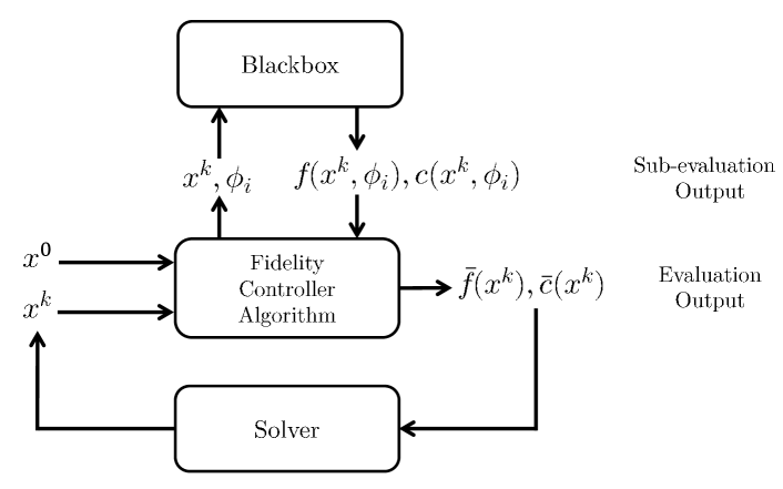
Figure 1: Optimization loop with the fidelity controller algorithm. The notation $\bar{f}(x)$ and $\bar{c}(x)$ indicate the output values at $x\in X$ at the last fidelity used by the algorithm.

Performing interruptions saves time when comparing to an optimization method in which each evaluation constitutes a single blackbox call with $\phi=1$. However, evaluating a feasible point involves potentially numerous sub-evaluations, significantly increasing the computational cost. Thus, defining the biadjacency matrix requires careful consideration. In counterpart, prioritizing time-saving by assigning constraints at low fidelities while choosing this matrix carries the risk of misidentifying the feasibility of a point with an early interruptions.

The matrix $B$ can be such that no constraint is assigned to $\phi=1$, meaning the true output values are never assessed. However, the scenario where the best solution given to the user by the solver at the end of an optimization is said to be feasible but is actually not is highly undesirable. Hence, the algorithm also considers $f^{*}_{k}$, the value of the best feasible solution after evaluating $x^{k}$. Whenever a point $x^{k}$ that has not been sub-evaluated with $\phi=1$ is about to be labeled as the best solution so far by the solver, an additional sub-evaluation with $\phi=1$ is introduced to ensure the feasibility of $x^{k}$.

Algorithm 1 shows the fidelity controller algorithm, without the evaluation superscripts $k$ as they are not relevant to the algorithm. When values are returned before the algorithm’s last line, the evaluation is said to be interrupted. An optimization from a solver using Algorithm 1 constitutes the third step of the hierarchically constrained optimization algorithm.

Algorithm 3.1: Fidelity controller
$\textbf{Input: }\text{ trial point }x;\text{ adjacency matrix }B;\text{ incumbent value }f^{*}$
$\textbf{For each fidelity }\phi_{i}\in\Phi\text{ to which at least one constraint is assigned}$
$\left.\middle|\begin{array}[]{l}\textbf{Evaluate }f(x,\phi_{i})\text{ and }c(x,\phi_{i})\text{, }\textbf{Store }\text{the values in $\bar{f}$ and $\bar{c}$.}\\ \textbf{If }c_{j}(x,\phi_{i})>0\text{ for some }j\in J\text{ where }B_{aj}=1\textbf{ for some }a\leq i\\ \left.\middle|\begin{array}[]{l}\textbf{Return }\bar{f},\bar{c}\end{array}\right.\\ \end{array}\right.$
$\textbf{If }\text{no constraint is assigned to $\phi_{L}$ and }f<f^{*}$
$\left.\middle|\begin{array}[]{l}\textbf{Evaluate }f(x,1)\text{ and }c(x,1)\text{, }\textbf{Store }\text{the values in $\bar{f}$ and $\bar{c}$.}\end{array}\right.$
$\textbf{Return }\bar{f},\bar{c}$

3.2 Computing method for the biadjacency matrix

This section introduces a computing method for the matrix $B$ which is broken down into two parts. First, a constraints behaviour in accordance with fidelity analysis is proposed. This process requires parallel computing to evaluate LH samples. Second, this behaviour analysis is used to construct a $B$ matrix.

3.2.1 Constraint behaviour analysis

The user selects a sample size $n_{H}$. If a starting point $x^{0}$ is provided, the LH bounds are centered around $x^{0}$ in order to analyse the constraint’s behaviour where the optimization is likely to take place. A new optimization parameter $\rho\in[0,1]$ named the Latin hypercube sizing factor is introduced to indicate the size of the sampled region. When $\rho=1$, the region is equal to $X=[\ell,u]$, and smaller values correspond to smaller regions. The centered LH bounds $(\ell^{\text{cen}},u^{\text{cen}})$ contain the following elements:

$$\ell^{\text{cen}}_{i}= \,\text{max}\left(\ell_{i},\ x^{0}_{i}-{\rho}(u_{i}-\ell_{i})\right)\quad\forall\,i\in\{1,2,\dots,n\}$$ (1)

$$u^{\text{cen}}_{i}= \,\text{min}\left(u_{i},\ x^{0}_{i}+{\rho}(u_{i}-\ell_{i})\right)\quad\forall\,i\in\{1,2,\dots,n\}.$$ (2)

If no starting point is provided, the LH bounds are simply those of $X$. Let $H\subset X$ denote the set of LH points, and let $H^{ap}\subseteq H$ be the subset containing all sampled points which do not violate any a priori constraint. Denote the cardinality of $H^{ap}$ by $n^{ap}$. Finally, define $I=\{1,2,\dots,L\}$ and the indicator function

$${\mathbbm{1}}(c_{j}(x,\phi)):=\left\{\begin{array}[]{l}0\qquad\text{ if }c_{j}(x,\phi)\leq 0\\ 1\qquad\text{ otherwise}\end{array}\right.\\ \qquad\forall j\in J.$$

A fidelity $\phi_{i}\in\Phi$ is said to be representative for a constraint $c_{j}\leq 0$ at a point $x$ if and only if

$${\mathbbm{1}}(c_{j}(x,\phi))={\mathbbm{1}}(c_{j}(x,1))\quad\forall\phi\in\Phi\text{ with }\phi\geq\phi_{i}.$$

This definition allows to identify fidelities at which a sub-evaluation correctly identifies whether a constraint is violated or not on the LH samples. The behaviour of the constraints in accordance with fidelity is characterized in two ways: the likeliness of a constraint to be violated at a given fidelity at any point during the optimization, and the likeliness of a fidelity to be representative for a given constraint at any point during the optimization. Another point of interest is the expected sub-evaluation time for the fidelities in $\Phi$. Define

$$r_{ij}:=\, Pr[\text{fidelity $\phi_{i}$ is representative for constraint $c_{j}\leq 0$ at some }x\in X]\quad \forall i\in I\,,\forall j\in J$$

$$p_{ij}:=\, Pr[c_{j}(x,\phi_{i})>0\mbox{ for some }x\in X] \forall i\in I\,,\forall j\in J$$

$$t_{i}:=\, \mathbb{E}_{x}[t(x,\phi_{i})] \forall i\in I.$$

Assuming that $t(x,\phi)$ is monotone increasing with $\phi$ for each $x\in X$,

$$t_{a}\leq t_{b}\quad\forall a,b\in I\text{ where }a<b.$$ (3)

After the LH samples are evaluated at each fidelity in $\Phi$, these statistical values are estimated with the following ratios:

$$r_{ij}\simeq\hat{r}_{ij}:=\, \frac{1}{n^{ap}}\lvert\{x\in\text{H}^{ap}:\phi_{i}\text{ is representative for }c_{j}\leq 0\}\lvert\quad \forall i\in I\,,\forall j\in J$$ (4)

$$p_{ij}\simeq\hat{p}_{ij}:=\, \frac{1}{n^{ap}}\lvert\{x\in\text{H}^{ap}:c_{j}(x,\phi_{i})>0\}\lvert \forall i\in I\,,\forall j\in J$$ (5)

$$t_{i}\simeq\hat{t}_{i}:=\, \frac{1}{n^{ap}}\sum_{x\in\text{H}^{ap}}t(x,\phi_{i}) \forall i\in I.$$ (6)

This characterization of the constraint’s behaviour constitute the first step of the hierarchically constrained optimization algorithm.

3.2.2 Optimal biadjacency matrix model

A biadjacency matrix is computed based on given values of $r_{ij}$, $p_{ij}$ and $t_{i}$. An explicit optimization Problem $\mathcal{Q}$ is proposed below to compute $B$, which minimizes the expected evaluation time during the optimization. It is also desired to minimize the probability of causing an interruption on a feasible point, but a bi-objective model is avoided by introducing a new threshold parameter $\varepsilon\in[0,1]$, the upper bound on the probability that a constraint’s feasibility is misidentified during the optimization. Every element $B_{ij}$ of the biadjacency matrix $B$ corresponds to a decision variable in the model. The $y_{i}$ variables are defined as follows. They are continuous variables in $\mathcal{Q}$ per their unimodality.

$$y_{i}=\begin{cases}1&\text{ if a sub-evaluation at fidelity\leavevmode\nobreak\ $\phi_{i}$ would be executed by Algorithm\leavevmode\nobreak\ \ref{algo:sous_eval_inter}}\\ 0&\text{ otherwise.}\end{cases}$$ (7)

In $\mathcal{Q}$, the objective function (10) represents the expected evaluation time of a single point according to Algorithm 1. It is a sum of all the sub-evaluation times $t_{i}$, multiplied by their probability of happening, which is the probability that no interruption happen earlier in the hierarchy multiplied by $y_{i}$ for each $i\in I$. It can be written as follows.

$$t_{1}y_{1}$$

$$+t_{2}y_{2}Pr[\text{no interruption at }\phi_{1}]$$

$$+t_{3}y_{3}Pr[\text{no interruption at }\phi_{1}]Pr[\text{no interruption at }\phi_{2}]$$

$$+t_{4}y_{4}Pr[\text{no interruption at }\phi_{1}]Pr[\text{no interruption at }\phi_{2}]Pr[\text{no interruption at }\phi_{3}]$$

$$+\dots$$

$$=\ t_{1}y_{1}+\sum_{i=2}^{L}\left(t_{i}y_{i}\prod_{k=1}^{i-1}Pr[\text{no interruption at }\phi_{k}]\right).$$ (8)

An index $k$ denotes a fidelity index smaller than or equal to a given $i\in I$. The probability that no interruption happens at a sub-evaluation at $\phi_{k}$ is the probability that all constraints assigned to $\phi_{k}$ are satisfied after the sub-evaluation. Under the hypothesis that these probabilities are independent, the product of each $(1-p_{kj})$ where $B_{kj}=1$ for each $j\in J$ is computed. Therefore,

$$P_{k}(B):=Pr[\text{no interruption at }\phi_{k}]=\prod_{j\in J}1-p_{kj}B_{kj}.$$ (9)

The substitution of (9) in (8) results in (10). Problem $\mathcal{Q}$ is defined as follows
$\mathcal{Q}$ $$\min_{B\in\mathbb{B}^{L\times m},y\in\mathbb{R}^{L}}\quad f(B)=t_{1}y_{1}+\sum_{i=2}^{L}t_{i}y_{i}\prod_{k=1}^{i-1}P_{k}(B)$$ (10) s.t. $\displaystyle\sum_{i\in I}B_{ij}=1\quad$ $\displaystyle\forall\,j\in J$ (11) $\displaystyle B_{ij}-\varepsilon\leq r_{ij}\quad$ $\displaystyle\forall\,i\in I,\,\forall\,j\in J$ (12) $\displaystyle B_{ij}\leq y_{i}\leq 1\quad$ $\displaystyle\forall\,i\in I,\,\forall\,j\in J$ (13) $\displaystyle y_{i}\leq\sum_{j\in J}B_{ij}\quad$ $\displaystyle\forall\,i\in I.$ (14)

Equation (11) ensures that every blackbox constraint is assigned to exactly one fidelity, Equation (12) enforces the $\varepsilon$ upper bound, and Equations (13) and (14) ensure the $y_{i}$ variables respect their definition (7).

The potential extra sub-evaluation at $\phi=1$ if the evaluated point is about to become the best solution so far is not considered, as the moments when it happens are unpredictable. Also, by calculating the estimations with the points from $H^{ap}$, the a priori constraints are disregarded by the model, which is not a problem because they have no impact on the optimal biadjacency matrix. A hypothesis assumed by this model is that if a constraint is satisfied at the fidelity it is assigned to, it is also satisfied at any greater fidelity.

3.3 Solving the model

Notice that Problem $\mathcal{Q}$ is mixed-integer with a polynomial objective function. As today’s solvers require a lot of solving time and have no guarantee of optimality for such problems, an alternative solving method is proposed. Indeed, the set of possible solutions may be reduced to the point where a simple exhaustive search is sufficient.

3.3.1 Reduction by introducing non-differentiability

The first reduction consists of simplifying the model by introducing non-differentiable elements, which are allowed since only an exhaustive search will be conducted. First, the $y_{i}$ variables are determined by the biadjacency matrix as:

$$y_{i}(B)=\left\{\begin{array}[]{ll}0&\text{ if }\sum\limits_{j\in J}B_{ij}=0\\ 1&\text{ otherwise}\end{array}\right.\quad\forall i\in I.$$

Hence, Equations (13) and (14) are removed, and a $B$ matrix alone constitutes a solution to the model. The function $i:J\rightarrow I$ is introduced, which returns the index of the smallest fidelity in $\Phi$ where constraint $c_{j}\leq 0$ can be assigned without violating Equation (12):

$$i(j)=\text{min}\{i\in I:r_{ij}\geq 1-\varepsilon\}.$$

Equation (12) is then equivalent to imposing that a constraint $c_{j}\leq 0$ can not be assigned to a fidelity $\phi_{i}$ when $i<i(j)$. These new definitions allow for the definition of Problem $\mathcal{Q}_{1}$, which is equivalent to $\mathcal{Q}$.

$\mathcal{Q}_{1}$

$$\min_{B\in\mathbb{B}^{L\times m}}\quad t_{1}y_{1}(B)+\sum_{i=2}^{L}\left(t_{i}y_{i}(B)\prod_{k=1}^{i-1}P_{k}(B)\right)$$

s.t. $$\sum_{i\in I}B_{ij}=1\quad \forall\,j\in J$$ (15)

$$B_{ij}=0\quad \forall\,(i,j)\in I\times J\mbox{ such that }i<i(j).$$ (16)

3.3.2 Reduction by filtering fidelities

The second reduction aims to reduce the number of rows of the biadjacency matrix $B$. It follows from Theorem 3.3.2, which indicates that there exists an optimal solution for $\mathcal{Q}_{1}$ where each constraint is assigned to a fidelity $\phi_{i}$ such that

$$i\in I_{F}:=\bigcup_{j\in J}i(j)\subseteq I,$$ (17)

with $I_{F}$ the filtered set of fidelity indexes. Each fidelity $\phi_{i}$ where $i\notin I_{F}$ can therefore be removed without excluding an optimal solution for $\mathcal{Q}_{1}$, by replacing $I$ with $I_{F}$. Note that $i(j)$ is a function that expresses a direct link between a fidelity index $i$ and a constraint index $j$. Conversely, the set $I_{F}$ removes that link. Theorem 3.3.2 states that an optimal solution exists where all constraints are assigned to fidelities $\phi_{i}$ where $i=i(j)$ for some $j\in J$, no matter what this $j$ is. The theorem is true under the assumption that probabilities $p_{ij}$ are monotonic decreasing with $i$ for each $i$ where constraint $c_{j}\leq 0$ can be assigned to fidelity $\phi_{i}$ without violating Equation (16), for each $j\in J$:

$$p_{aj}\geq p_{bj}\quad\forall j\in J,\,\forall a,b\in I\text{ where }i(j)\leq a<b.$$ (18)

The theorem can remain valid without this assumption. Indeed, as $\varepsilon$ becomes smaller, the likelihood of the theorem becoming invalid decreases [30].

Lemma 1 Let $B$ be a feasible solution for $\mathcal{Q}_{1}$. If there exists a fidelity index $i^{\prime}\in I\backslash I_{F}$ to which at least one blackbox constraint is assigned, then the matrix $B^{\prime}$ where

$$B^{\prime}_{ij}=\left\{\begin{array}[]{ll}0&\text{ if $i=i^{\prime}$}\\ 1&\text{ if $i=i^{\prime}-1$ and }B_{i^{\prime}j}=1\\ B_{ij}&\text{ otherwise}\end{array}\right.\qquad\forall i\in I,\,\forall j\in J$$ (19)

is feasible for $\mathcal{Q}_{1}$.
Proof. Let $B$ be a feasible solution for $\mathcal{Q}_{1}$ and $i^{\prime}\in I\backslash I_{F}$ be a fidelity index to which at least one blackbox constraint is assigned. Equation (15) is satisfied by $B^{\prime}$, because it is satisfied by $B$ and $B^{\prime}_{i^{\prime}-1\,j}+B^{\prime}_{i^{\prime}j}=1=B_{i^{\prime}-1\,j}+B_{i^{\prime}j}$ for each $j\in J$. Concerning Equation (16), on the one hand, if $(i,j)\in I\times J$ is such that $i<i(j)$, then $B_{ij}=0$ since $B$ is feasible. On the other hand, if $j^{\prime}\in J$ is such that $B_{i^{\prime}j^{\prime}}=1$ then $i^{\prime}>i(j^{\prime})$, which is equivalent to $i^{\prime}-1\geq i(j^{\prime})$. The last condition in Equation (19) ensures that $B^{\prime}_{ij}=B_{ij}=0$ for each pair $(i,j)\in I\times J$ such that $i<i(j)$, which implies that the matrix $B^{\prime}$ is feasible for $\mathcal{Q}_{1}$. $\square$

Lemma 2 Let $B$ be a feasible solution for $\mathcal{Q}_{1}$. Under Assumption (18), if there exists a fidelity index $i^{\prime}\in I\backslash I_{F}$ to which at least one blackbox constraint is assigned, then the matrix $B^{\prime}$ given by (19) satisfies $f(B^{\prime})\leq f(B)$.
Proof. Let $B$ be a feasible solution for $\mathcal{Q}_{1}$ and $i^{\prime}\in I\backslash I_{F}$ be a fidelity index to which at least one blackbox constraint is assigned. The objective function (10) maybe be divided into four terms, which correspond to the fidelity indexes smaller than $i^{\prime}-1$, equal to $i^{\prime}-1$, equal to $i^{\prime}$ and greater than $i^{\prime}$ of the sum

$$f(B)=T_{<i^{\prime}-1}(B)+T_{i^{\prime}-1}(B)+T_{i^{\prime}}(B)+T_{>i^{\prime}}(B)$$

where

$$T_{<i^{\prime}-1}(B)\ =\ t_{1}y_{1}(B)+\sum_{i=2}^{i^{\prime}-2}t_{i}y_{i}(B)\prod_{k=1}^{i-1}P_{k}(B), T_{i^{\prime}-1}(B)\ =\ t_{i^{\prime}-1}y_{i^{\prime}-1}(B)\prod_{k=1}^{i^{\prime}-2}P_{k}(B),$$

$$T_{i^{\prime}}(B)\ =\ t_{i^{\prime}}y_{i^{\prime}}(B)\prod_{k=1}^{i^{\prime}-1}P_{k}(B), T_{>i^{\prime}}(B)\ =\ \sum_{i=i^{\prime}+1}^{L}t_{i}y_{i}(B)\prod_{k=1}^{i-1}P_{k}(B).$$

Equation (19) ensures that the first term satisfies $T_{<i^{\prime}-1}(B)=T_{<i^{\prime}-1}(B^{\prime})$. Assumption (18) ensures that the last term satisfies $T_{>i^{\prime}}(B)\geq T_{>i^{\prime}}(B^{\prime})$, as the only change from $T_{>i^{\prime}}(B)$ to $T_{>i^{\prime}}(B^{\prime})$ is that all $p_{i^{\prime}j}$ become $p_{i^{\prime}-1\,j}$. For the two central terms, two cases are considered. First, if $y_{i^{\prime}-1}(B)=0$, then $T_{i^{\prime}-1}(B)=T_{i^{\prime}}(B^{\prime})=0$ as $y_{i^{\prime}}(B^{\prime})=0$. Furthermore, Assumption (3) ensures that

$$T_{i^{\prime}}(B)\ =\ t_{i^{\prime}}\prod_{k=1}^{i^{\prime}-1}P_{k}(B)\ =\ t_{i^{\prime}}\prod_{k=1}^{i^{\prime}-2}P_{k}(B^{\prime})\ \geq\ t_{i^{\prime}-1}\prod_{k=1}^{i^{\prime}-2}P_{k}(B^{\prime})\ =\ T_{i^{\prime}-1}(B^{\prime}).$$

Second, if $y_{i^{\prime}-1}(B)=1$, then $T_{i^{\prime}-1}(B)=T_{i^{\prime}-1}(B^{\prime})$ as the sub-evaluations at $\phi_{i^{\prime}-1}$ and at lower fidelities are unchanged, and $T_{i^{\prime}}(B)>T_{i^{\prime}}(B^{\prime})=0$ as $y_{i^{\prime}}(B^{\prime})=0$. In both cases, the sum of the four terms of $f(B)$ is greater than or equal to those of $f(B^{\prime})$. Consequently, $f(B)\geq f(B^{\prime})$. $\square$

Theorem 3 There exists an optimal solution for $\mathcal{Q}_{1}$ in which every blackbox constraint is assigned to a fidelity $\phi_{i}$ where $i\in I_{F}$.
Proof. The argmin of $\mathcal{Q}_{1}$ can possibly contain only solutions where every blackbox constraint is assigned to a fidelity $\phi_{i}$ where $i\in I_{F}$. The theorem is then trivial. Otherwise, there exists a solution $B^{*}_{0}$ in the argmin of $\mathcal{Q}_{1}$ such that the set

$$I^{\prime}(B^{*}_{0}):=\{i\in I\backslash I_{F}:y_{i}(B^{*}_{0})=1\}$$

is not empty. For a given $i^{\prime}\in I^{\prime}(B^{*}_{0})$, it is possible to find another solution, $B^{*}_{1}$, where every constraint assigned to $\phi_{i^{\prime}}$ is rather assigned to $\phi_{i^{\prime}-1}$, and where every other assignment is unchanged. Lemma 3.3.2 indicates that $B^{*}_{1}$ is feasible, and Lemma 3.3.2 indicates that it yields an equal or better objective function value than $B^{*}_{0}$. Therefore, $B^{*}_{1}$ is also part of the $\operatorname*{argmin}$. Then, the set $I^{\prime}(B^{*}_{1})$ can then be calculated. As long as $I^{\prime}$ is non-empty, this process is repeated to find $B^{*}_{2}$, $B^{*}_{3}$ and so on. The maximum number of such iterations is $\max\{L-i(j):j\in J\}$, implying this process always terminates. When it does in $K$ iterations, $I^{\prime}(B^{*}_{K})=\varnothing$, and $B^{*}_{K}$ is an optimal solution for $\mathcal{Q}_{1}$ in which every blackbox constraint is assigned to a fidelity belonging to $I_{F}$. $\square$

3.3.3 Reduction by filtering constraints

The third reduction simply consists of filtering out all a priori constraints, as they have no impact on the optimal biadjacency matrix. This reduces the number of columns of the biadjacency matrix $B$. The set $J$ is replaced for

$$J_{F}:=\{j\in J:c_{j}\leq 0\text{ is not an a priori constraint}\},$$ (20)

the set of filtered constraint indexes.

3.3.4 Exhaustive search

First, consider $\mathcal{Q}_{1}$, and replace $I$ for $I_{F}$ and $J$ for $J_{F}$, therefore removing columns and rows of variables from matrix $B$, and removing multiple $p_{ij}$, $r_{ij}$ and $t_{i}$ elements from the model. This new problem is named $\mathcal{Q}_{2}$. Equation (12) indicates that $B_{ij}=0$ if $r_{ij}<1-\varepsilon$. Equation (11) indicates that every constraint is assigned to exactly one fidelity. Every solution for Problem $\mathcal{Q}_{2}$ that satisfies these two equations is then exhaustively listed. For each solution, the objective function value is computed with (10), and an optimal solution is found. From this solution, an optimal biadjacency matrix $B^{*}$ of size $L\times m$ can be created by reintroducing columns $J\backslash J_{F}$ and rows $I\backslash I_{F}$, and by giving the value of 0 to these new elements. Computing an optimal assignment with the estimations $\hat{p}_{ij}$, $\hat{r}_{ij}$ and $\hat{t}_{i}$ rather than the true values which are unavailable constitutes the second step of the hierarchically constrained optimization algorithm.

3.4 Hierarchically constrained optimization algorithm

Now that every part of the hierarchically constrained optimization algorithm has been presented, see Algorithm 3.4 for the full algorithm. When constructing $\mathcal{Q}_{2}$ and $I_{F}$ during the algorithm, $r_{ij}$ and $p_{ij}$ are substituted by $\hat{r}_{ij}$, $\hat{p}_{ij}$ for each $i\in I$, and for each $j\in J$, and $t_{i}$ is substituted by $\hat{t}_{i}$ for each $i\in I$.

Algorithm 3.2: Hierarchically constrained optimization

Input:

$\left.\middle|\begin{array}[]{ll}x^{0}:&\text{optimization starting point (optional)}\\ \mathcal{P}:&\text{problem containing $X\subseteq{\mathbb{R}}^{n}$, $f$ and $c$}\\ \Phi:&\text{ordered set of fidelities ending with $1$}\\ \varepsilon:&\text{upper bound on the probability that a constraint's feasibility is misidentified}\\ \rho,n_{H}:&\text{Latin hypercube sizing factor and sample size}\\ \end{array}\right.$

1. Constraint behaviour in accordance with fidelity analysis.

$\left.\middle|\begin{array}[]{l}\textbf{If }x^{0}\text{ is provided, find the $(\ell^{\text{cen}},u^{\text{cen}})$ bounds from $X$, $\rho$ and $x^{0}$ using\leavevmode\nobreak\ \eqref{eq:licen} and\leavevmode\nobreak\ \eqref{eq:uicen}}.\\ \textbf{Else}\text{, set }(\ell^{cen},u^{cen})=(\ell,u)\text{ and at end of step 1, set $x^{0}$ as the best point in $H$.}\\ \text{Randomly determine $H$, the $n_{H}$ LH points bounded by $\ell^{cen}$ and $u^{cen}$.}\\ \text{Evaluate each point in $H$ at each fidelity in $\Phi$ by parallelizing as much as possible.}\\ \text{Calculate all $\hat{r}_{ij}$, $\hat{p}_{ij}$ and $\hat{t}_{i}$ estimations using\leavevmode\nobreak\ \eqref{eq:hatr},\leavevmode\nobreak\ \eqref{eq:hatp} and\leavevmode\nobreak\ \eqref{eq:hatt}, respectively.}\end{array}\right.$

2. Optimal biadjacency matrix computation.

$\left.\middle|\begin{array}[]{l}\text{Find $J_{F}$, and find $I_{F}$ with $\varepsilon$ using\leavevmode\nobreak\ \eqref{eq:hatJ} and\leavevmode\nobreak\ \eqref{eq:hatI}, respectively}.\\ \text{Solve problem $\mathcal{Q}_{2}$ with an exhaustive search on }\Omega.\\ \text{Create a matrix $B\in\mathbb{B}^{L\times m}$ from an optimal solution for }\mathcal{Q}_{2}.\\ \end{array}\right.$

3. Blackbox optimization.

$\left.\middle|\begin{array}[]{l}\text{Solve $\mathcal{P}$ with the chosen solver, providing Algorithm\leavevmode\nobreak\ \ref{algo:sous_eval_inter} with matrix $B$}\\ \quad\text{as the blackbox evaluation function and $x^{0}$ to the solver. Update $f^{*}_{k}$ at}\\ \quad\text{end of evaluation }k.\\ \end{array}\right.$

Return the solver output

4 Computational results

This section shows an application of Algorithm 3.4 with the NOMAD 4 software [14, 28]. It is not an in depth analysis, but rather a proof of concept of the theoretical method. Computing is done on Intel Xeon Gold 6150 CPU @ 2.70GHz processors. The benchmark problems are sourced from the solar family of blackboxes [31]. As far as the authors are aware, solar is the only benchmarking blackbox collection of problems where constraints that are affected by fidelity can be found. Hence, benchmarking is only conducted on problems from this collection. In NOMAD, constraints can be managed using the EB or the PB methods. Literature suggests that the PB generally yields better results. However, due to Algorithm 1 not returning the true outputs when the evaluation of a point is interrupted, the EB might be more adapted, as it rejects these points. Conversely, the PB uses output values to compute new incumbent points. Therefore, two implementations and a base case are tested for comparison:

• Inter PB: Algorithm 3.4 with NOMAD and the PB;

• Inter EB: Algorithm 3.4 with NOMAD and the EB;

• Base case: NOMAD with default parameters and blackbox fidelity fixed at 1.

The method introduced in this paper is motivated by computationally expensive problems, such as PRIAD’s blackbox, where the solver and the Algorithm 1 computation times are insignificant in comparison. To replicate such problems with solar instances that are computationally less demanding but possess desirable characteristics, only blackbox computation times are considered in the following profiles. For both implementations of the algorithm, the empirically determined values of $n_{H}=10^{4}$, $\varepsilon=0.05$ and

$$\Phi=\{10^{-10},2^{-10},2^{-9},2^{-8},2^{-7},2^{-6},2^{-5},2^{-4},0.1,0.2,0.3,0.4,0.5,0.6,0.7,0.8,0.9,1\}$$

are chosen.

4.1 Without a starting point for the optimization

This section presents optimizations where no starting point is provided by the user. Consequently, the LH bounds are those of $X$. The base case also performs a LH with the same parameters to find a starting point. Optimizations on three constrained multi-fidelity instances of the solar family of blackboxes: solar2, solar3 and solar4 are conducted. By varying the unfeasible starting point, 20 optimization runs are executed for each tested instance. The results are illustrated in data profiles, with the initial two profiles relating to solar2, and shown in Figure 2. As the LH times are identical, only the optimization times are shown.

(a) $\tau=0.0001$

(b) $\tau=0.001$

Figure 2: solar2 data profiles from 20 runs with no $x^{0}$.

The Algorithm 3.4’s success, whether paired with the EB or the PB, is mainly attributed to two factors. Firstly, solar2 contains a frequently violated constraint with a high estimated probability of representativity at low fidelities, which allows for numerous quick interruptions on infeasible points. Secondly, the calculated $B$ matrix is accurate because the constraint’s behaviour is homogeneous throughout $X$. On the other hand, this is not the case for solar3 and solar4, where the calculated $B$ matrix does not accurately reflect the constraint’s behaviour for the encountered points during optimization. The results show that when using Algorithm 3.4, every evaluated point is systematically considered infeasible. No figures are shown as there are no curves for the 3.4 implementations. Conversely, the base case finds numerous feasible solutions.

4.2 With a starting point for the optimization

This section presents optimizations where a known feasible starting point is provided by the user. The optimization runs are conducted on each constrained multi-fidelity instances of the solar family of blackboxes: solar2, solar3, solar4 and solar7, with $\rho$ values of $\frac{1}{4}$, $\frac{1}{10}$, $\frac{1}{20}$ and $\frac{1}{4}$ respectively. Those values are based on preliminary results. In this scenario, the base case does not perform any LH sampling, which grants it a time advantage. However, this advantage is inconsequential due to the extensive parallelization of samples using Hydro-Québec’s facilities. By varying the NOMAD seed for random polls, 20 optimization runs are executed for each tested instance, and the results are illustrated in data profiles. Two data profiles for solar2 are shown in Figure 3.

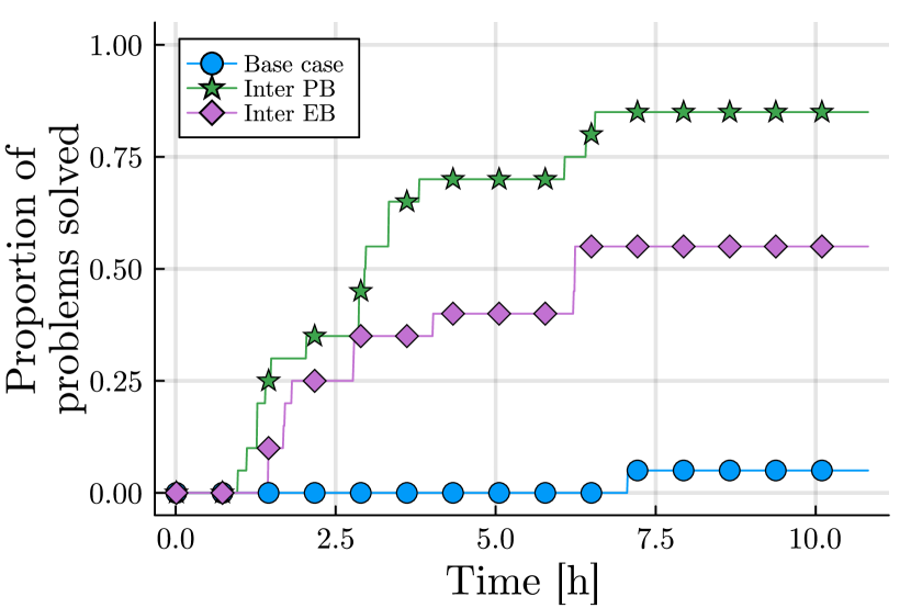
(a) $\tau=0.1$

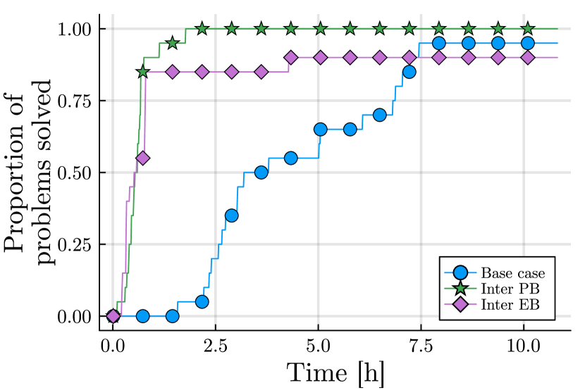
(b) $\tau=0.5$

Figure 3: solar2 data profiles with a starting point. Curves from implementations of Algorithm 3.4 start at 642.22 seconds to account for LH sampling time.

With $\tau=0.5$, the base case solves a greater number of problems compared to the proposed algorithm with the EB, as the implementation is highly inefficient for one of the 20 optimization runs. In general, both implementations of Algorithm 3.4 are preferable.

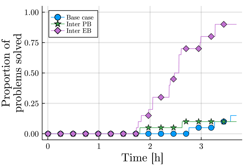
(a) $\tau=0.05$

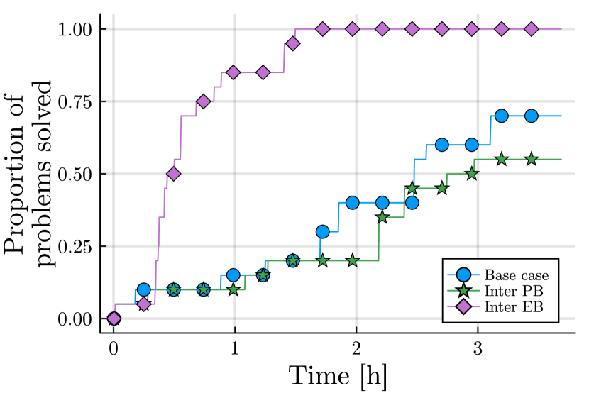
(b) $\tau=0.3$

Figure 4: solar3 data profiles from 20 runs with a given $x^{0}$. Curves from implementations of Algorithm 3.4 start at 45.64 seconds to account for LH sampling time.

Data profiles for solar3 and solar4 are shown in Figure 4 and Figure 5, respectively.

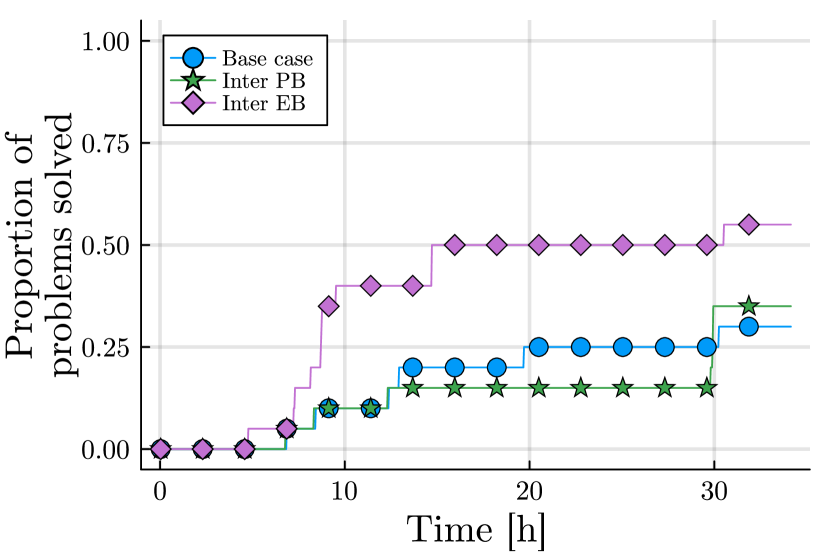
(a) $\tau=0.01$

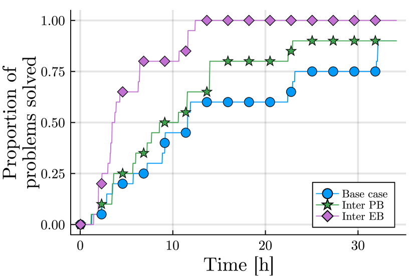
(b) $\tau=0.1$

Figure 5: solar4 data profiles from 20 runs with a given $x^{0}$. Curves from implementations of Algorithm 3.4 start at 94.75 seconds to account for LH sampling time.

For both instances, the base case yields results comparable to Algorithm 3.4 paired with the PB. On the other hand, when pairing the algorithm with the EB, it performs significantly better. This can be attributed to a higher scarcity of feasible points in solar3 and solar4 compared to solar2. This section also studies solar7, a constrained multi-fidelity blackbox where infeasible points are much less common than for the other tested instances. It serves as a test to assess how Algorithm 3.4 performs when it has limited opportunities to interrupt evaluations and save time in contrast to the base case. Additionally, the objective function value is affected by multi-fidelity for this instance. Thus, the condition $y_{L}=1$ is imposed. Results show that the optimal biadjacency matrix computed for this problem assigns all constraints to $\phi_{L}=1$. This suggests that the method has discerned the absence of meaningful opportunities for interruptions and that emulating the base case is the optimal approach. No figure is shown; the base case and the PB implementation exhibit identical data profiles, except for the fact that the base case consistently precedes by 181.07 seconds due to its absence of LH sampling prior to any optimization.

5 Discussion

We have introduced a novel approach to computationally expensive multi-fidelity blackbox optimization problems by leveraging low-fidelity assessments of constraints violation to interrupt evaluations. Our computational results demonstrate that, under specific conditions, pairing the NOMAD solver with the hierarchically constrained optimization algorithm yields significantly superior solutions compared to NOMAD alone. Here is a summary of favorable conditions:

• scarce feasible points;

• accurate constraint violation assessments at lower fidelity levels;

• homogeneity in constraint behaviour relative to fidelity within the LH bounds defined by the sizing factor $\rho$.

When this final condition is not fulfilled with $\rho=1$, the existence of a known feasible solution prior to the optimization becomes vital; it enables the selection of a sizing factor $\rho$ that increases the homogeneity in constraint behaviour.

When utilizing the NOMAD solver, we observe that the preferred barrier choice depends on the blackbox. For problems with infrequent feasible points, the EB is more suitable, while the PB is mostly preferred when feasible points are more common.

Future work involve dynamically computing the biadjacency matrix and applying the proposed algorithm to complex industrial problems, such as PRIAD’s. Additionally, as indicated by [6, 33], the constraint behaviour analysis can potentially be improved with machine learning methods.

Data availability and conflict of interest statement

The solar problems are available at https://github.com/bbopt/solar. The NOMAD software package is available at https://github.com/bbopt/nomad. This work has been funded by the NSERC Discovery grants of C. Audet (#2020-04448) and S. Le Digabel (#2018-05286), by the NSERC/Mitacs Alliance grant (#571311-21) in collaboration with Hydro-Québec, and by X. Lebeuf’s NSERC Graduate Scholarships – Master’s grant.

References

- [1] A. Agrawal, K. Ravi, P.S. Koutsourelakis, and H.J. Bungartz. Multi-fidelity Constrained Optimization for Stochastic Black Box Simulators. Technical Report 2311.15137, ArXiv, 2023.
- [2] S. Alarie, C. Audet, P.-Y. Bouchet, and S. Le Digabel. Optimisation of stochastic blackboxes with adaptive precision. SIAM Journal on Optimization, 31(4):3127–3156, 2021.
- [3] S. Alarie, C. Audet, P. Jacquot, and S. Le Digabel. Hierarchically constrained blackbox optimization. Operations Research Letters, 50(5):446–451, 2022.
- [4] E. Alba, G. Luque, and S. Nesmachnow. Parallel metaheuristics: recent advances and new trends. International Transactions in Operational Research, 20(1):1–48, 2013.
- [5] N. Andrés-Thió, M.A. Muñoz, and K. Smith-Miles. Bifidelity Surrogate Modelling: Showcasing the Need for New Test Instances. INFORMS Journal on Computing, 34(6):3007–3022, 2022.
- [6] C. Audet, G. Caporossi, and S. Jacquet. Binary, unrelaxable and hidden constraints in blackbox optimization. Operations Research Letters, 48(4):467–471, 2020.
- [7] C. Audet and J.E. Dennis, Jr. A pattern search filter method for nonlinear programming without derivatives. SIAM Journal on Optimization, 14(4):980–1010, 2004.
- [8] C. Audet and J.E. Dennis, Jr. Mesh Adaptive Direct Search Algorithms for Constrained Optimization. SIAM Journal on Optimization, 17(1):188–217, 2006.
- [9] C. Audet and J.E. Dennis, Jr. A Progressive Barrier for Derivative-Free Nonlinear Programming. SIAM Journal on Optimization, 20(1):445–472, 2009.
- [10] C. Audet, J.E. Dennis, Jr., and S. Le Digabel. Globalization strategies for Mesh Adaptive Direct Search. Computational Optimization and Applications, 46(2):193–215, 2010.
- [11] C. Audet, K.J. Dzahini, M. Kokkolaras, and S. Le Digabel. Stochastic mesh adaptive direct search for blackbox optimization using probabilistic estimates. Computational Optimization and Applications, 79(1):1–34, 2021.
- [12] C. Audet and W. Hare. Derivative-Free and Blackbox Optimization. Springer Series in Operations Research and Financial Engineering. Springer, Cham, Switzerland, 2017.
- [13] C. Audet, A. Ihaddadene, S. Le Digabel, and C. Tribes. Robust optimization of noisy blackbox problems using the Mesh Adaptive Direct Search algorithm. Optimization Letters, 12(4):675–689, 2018.
- [14] C. Audet, S. Le Digabel, V. Rochon Montplaisir, and C. Tribes. Algorithm 1027: NOMAD version 4: Nonlinear optimization with the MADS algorithm. ACM Transactions on Mathematical Software, 48(3):35:1–35:22, 2022.
- [15] A. Bayoumy and M. Kokkolaras. A Relative Adequacy Framework for Multi-model Management in Design Optimization. ASME Journal of Mechanical Design, pages 1–22, 2020.
- [16] A. Bayoumy and M. Kokkolaras. A relative adequacy framework for multimodel management in multidisciplinary design optimization. Structural and Multidisciplinary Optimization, 62(4):1701–1720, 2020.
- [17] A. Bayoumy and M. Kokkolaras. Multi-model management for time-dependent multidisciplinary design optimization problems. Structural and Multidisciplinary Optimization, 61(5):1821–1841, 2020.
- [18] A. Côté, O. Blancke, S. Alarie, A. Dems, D. Komljenovic, and D. Messaoudi. Combining Historical Data and Domain Expert Knowledge Using Optimization to Model Electrical Equipment Reliability. In 2020 International Conference on Probabilistic Methods Applied to Power Systems (PMAPS), pages 1–6, Liege, Belgium, 2020.
- [19] K.J. Dzahini. Expected complexity analysis of stochastic direct-search. Computational Optimization and Applications, 81(1):179–200, 2022.
- [20] M.G. Fernández-Godino. Review of multi-fidelity models. Technical Report 1609.07196, ArXiv, 2023.
- [21] R. Fletcher and S. Leyffer. Nonlinear programming without a penalty function. Mathematical Programming, Series A, 91:239–269, 2002.
- [22] R. Fletcher, S. Leyffer, and Ph.L. Toint. A brief history of filter methods. SIAM SIAG/OPT Views-and-News, 18(1):2–12, 2006.
- [23] M. Gaha, B. Chabane, D. Komljenovic, A. Côté, C. Hébert, O. Blancke, A. Delevari, and G.Abdul-Nour. Global Methodology for Electrical Utilities Maintenance Assessment Based on Risk-Informed Decision Making. Sustainability, 13(16):9091, 2021.
- [24] G.A. Gray and T.G. Kolda. Algorithm 856: APPSPACK 4.0: Asynchronous parallel pattern search for derivative-free optimization. ACM Transactions on Mathematical Software, 32(3):485–507, 2006.
- [25] R.T. Haftka, D. Villanueva, and A. Chaudhuri. Parallel surrogate-assisted global olptimization with expensive functions – a survey. Structural and Multidisciplinary Optimization, 54(1):3–13, 2016.
- [26] M.D. Hill and M.R. Marty. Amdahl’s Law in the Multicore Era. Computer, 41(7):33–38, 2008.
- [27] D. Komljenovic, D. Messaoudi, A. Côté, M. Gaha, L. Vouligny, S. Alarie, A. Dems, and O. Blancke. Asset Management in Electrical Utilities in the Context of Business and Operational Complexity. In 14th WCEAM Proceedings, pages 34–45, 2021.
- [28] S. Le Digabel. Algorithm 909: NOMAD: Nonlinear Optimization with the MADS algorithm. ACM Transactions on Mathematical Software, 37(4):44:1–44:15, 2011.
- [29] S. Le Digabel and S.M. Wild. A taxonomy of constraints in black-box simulation-based optimization. Technical Report G-2015-57, Les cahiers du GERAD, 2023. To appear in Optimization and Engineering.
- [30] X. Lebeuf. Optimisation de boîtes noires multifidélités avec contraintes hiérarchisées. Master’s thesis, Polytechnique Montréal, 2023. Available at https://publications.polymtl.ca/53386/.
- [31] M. Lemyre Garneau. Modelling of a solar thermal power plant for benchmarking blackbox optimization solvers. Master’s thesis, Polytechnique Montréal, 2015. Available at https://publications.polymtl.ca/1996/.
- [32] M.D. McKay, R.J. Beckman, and W.J. Conover. A comparison of three methods for selecting values of input variables in the analysis of output from a computer code. Technometrics, 21(2):239–245, 1979.
- [33] M. Menz, M. Munoz-Zuniga, and D. Sinoquet. Estimation of simulation failure set with active learning based on Gaussian Process classifiers and random set theory. Technical Report hal-03848238, IFPEN – IFP Energies nouvelles, 2023.
- [34] J. Müller and J. Woodbury. GOSAC: global optimization with surrogate approximation of constraints. Journal of Global Optimization, 69(1):117–136, 2017.
- [35] B. Peherstorfer, K. Willcox, and M. Gunzburger. Survey of Multifidelity Methods in Uncertainty Propagation, Inference, and Optimization. SIAM Review, 60(3):550–591, 2018.
- [36] E. Polak and M. Wetter. Precision control for generalized pattern search algorithms with adaptive precision function evaluations. SIAM Journal on Optimization, 16(3):650–669, 2006.
- [37] S. Razavi, B. Tolson, L. Matott, N. Thomson, A. MacLean, and F. Seglenieks. Reducing the computational cost of automatic calibration through model preemption. Water Resources Research, 46(11), 2010.
- [38] R. Sen, K. Kandasamy, and S. Shakkottai. Multi-fidelity black-box optimization with hierarchical partitions. International conference on machine learning, 80:4538–4547, 2018.
- [39] H. Wang, Y. Jin, and J. Doherty. A Generic Test Suite for Evolutionary Multifidelity Optimization. IEEE Transactions on Evolutionary Computation, 22(6):836–850, 2018.
- [40] M. Wetter and E. Polak. Building design optimization using a convergent pattern search algorithm with adaptive precision simulations. Energy and Buildings, 37(6):603–612, 2005.