Associated production of heavy quarkonium and $D-$meson in the improved color evaporation model with KaTie

Abstract

In the article, we study associated production of prompt $J/\psi(\Upsilon)$ and $D-$mesons in the improved color evaporation model using the high-energy factorization approach as it is realized in the Monte-Carlo event generator KaTie. The modified Kimber-Martin-Ryskin-Watt model for unintegrated parton distribution functions is used. We predict cross sections for associated $J/\psi(\Upsilon)$ and $D-$meson hadroproduction via the single and double parton scattering mechanisms using the set of model parameters which has been fixed early for description of prompt single and pair heavy quarkonium production at the LHC energies. We found the results of calculations agree with the LHCb Collaboration data at the energies $\sqrt{s}=7,8$ TeV and we present theoretical predictions for the energy $\sqrt{s}=13$ TeV .

I Introduction

Measurements of the $J/\psi+D$ and $\Upsilon+D$ (here and below $\Upsilon=\Upsilon(1S)$) associated production by the LHCb Collaboration Aaij et al. (2012, 2016) at the energies $\sqrt{s}=7,8$ TeV clear demonstrate a dominant role of the double parton scattering (DPS) mechanism of the parton model compared with the conventional single parton scattering (SPS) scenario. The average value of the DPS parameter $\sigma_{eff}$ extracted in the $\Upsilon+D$ pair production is about $\sigma_{eff}=18.0\pm 1.8$ mb and in the $J/\psi+D$ it is about $\sigma_{eff}=15.8\pm 2.4$ mb  Aaij et al. (2012, 2016). For today, the extractions of parameter $\sigma_{\rm eff}$, based on the DPS pocket formula Calucci and Treleani (1999), have been obtained in different experiments. Values of $\sigma_{\rm eff}=2-25$ mb have been derived, though with large errors, with a simple average giving $\sigma_{\rm eff}=15$ mb  Chapon et al. (2022).

Theoretical calculations performed in the leading order (LO) in $\alpha_{S}$ of the collinear parton model within the Color Singlet Model Baier and Ruckl (1983); Berger and Jones (1981) and within the approach of the Nonrelativistic Quantum Chromodynamics (NRQCD) Bodwin et al. (1995) predict very small values of the SPS cross sections for $J/\psi+D$ Shao (2020) and $\Upsilon+D$ pair production Berezhnoy and Likhoded (2015); Likhoded et al. (2016). In the Ref. Karpishkov et al. (2019), the associated $\Upsilon+D$ pair production was studied in the $k_{T}-$factorization Collins and Ellis (1991); Catani and Hautmann (1994); Gribov et al. (1983) and NRQCD and it was demonstrated that SPS contribution to the cross section is also sufficiently smaller the experimental data from LHCb collaboration Aaij et al. (2016). The new LHCb measurements of $J/\psi+J/\psi$ and $J/\psi+\Upsilon$ pair production cross sections Aaij et al. (2023a, b) motivate to make predictions for $J/\psi+D$ and $\Upsilon+D$ pair production at the $\sqrt{s}=7$ and $13$ TeV. Instead of previous theoretical studies for such processes, we use Improved Color Evaporation Model (ICEM) Ma and Vogt (2016) to describe hadronization of heavy quark and antiquark pair into a final quarkonium. The ICEM was successfully used recently to describe single $J/\psi(\Upsilon)$ production both in the collinear parton model Cheung and Vogt (2017, 2021) and in the $k_{T}-$factorization Cheung and Vogt (2018); Maciuła et al. (2019). The pair quarkonium production in the ICEM using the $k_{T}-$factorization was studied in Refs. Chernyshev and Saleev (2022); Saleev and Chernyshev (2023). The D-meson production at the LHC energies was described in the $k_{T}-$factorization and the fragmentation approach using $c\to D$ nonperturbative fragmentation function $D_{c\to D}(z)$ in Refs.Maciuła et al. (2016); van Hameren et al. (2015).

In the study, we calculate cross section for associated $J/\psi+D$ and $\Upsilon+D$ production in the proton-proton collisions in the $k_{T}$-factorization Collins and Ellis (1991); Catani and Hautmann (1994); Gribov et al. (1983) using the Monte-Carlo (MC) event generator KaTie van Hameren (2018). Following by the parton Reggeization approach (PRA) Karpishkov et al. (2017); Nefedov and Saleev (2020), which is a gauge-invariant version of the $k_{T}-$factorization, the modified Kimber-Martin-Ryskin-Watt model  Kimber et al. (2001); Watt et al. (2003) for unintegrated parton distribution functions (uPDFs) is used Nefedov and Saleev (2020).

II Event generator KaTie and unintegrated parton distribution functions

We apply fully numerical method of the calculation using the parton level event generator KaTie van Hameren (2018). The approach to obtaining gauge invariant amplitudes with off-shell initial state partons in scattering at high-energy multi-Regge kinematics was proposed in the Ref. van Hameren et al. (2013a, b). The method is based on the use of spinor amplitudes formalism and recurrence relations of the Britto-Cachazo-Feng-Witten (BCFW) type. This formalism van Hameren (2018); van Hameren et al. (2013a, b) for numerical amplitude generation is equivalent to amplitudes built according to Feynman rules of the Lipatov Effective Field Theory at the level of tree diagrams Nefedov et al. (2013); Kutak et al. (2016). The accuracy of numerical calculations using KaTie for total proton-proton cross sections is taking as 0.1 %.

In the high-energy factorization or $k_{T}-$factorization, the cross section for the hard process $p+p\to{\cal Q}+X$ in the multi-Regge kinematics is calculated as integral convolution of the parton cross section $d\hat{\sigma}(i+j\to{\cal Q}+X)$ and the unintegrated parton distribution functions (uPDFs) by the factorization formula

$$d\sigma = \sum_{i,\bar{j}}\int\limits_{0}^{1}\frac{dx_{1}}{x_{1}}\int\frac{d^{2}{\bf q}_{T1}}{\pi}{\Phi}_{i}(x_{1},t_{1},\mu^{2})\int\limits_{0}^{1}\frac{dx_{2}}{x_{2}}\int\frac{d^{2}{\bf q}_{T2}}{\pi}{\Phi}_{j}(x_{2},t_{2},\mu^{2})\cdot d\hat{\sigma},$$ (1)

where $t_{1,2}=-{\bf{q}}_{1,2T}^{2}$, $q_{1,2}^{\mu}=x_{1,2}P_{1,2}^{\mu}+q_{1,2T}^{\mu}$, $q_{1,2T}=(0,{\bf{q}}_{1,2T},0)$, the cross section of the subprocess with off-shell initial partons, which are treated as Reggeized partons Lipatov (1995); Lipatov and Vyazovsky (2001), $d\hat{\sigma}$ is expressed in terms of squared Reggeized amplitudes $\overline{|{\mathcal{A}}_{\mathrm{PRA}}|^{2}}$ in a standard way Nefedov et al. (2013).

The unPDFs can be written as follows from the KMRW model Kimber et al. (2001); Watt et al. (2003):

$$\Phi_{i}(x,t,\mu^{2})=\frac{\alpha_{s}(\mu)}{2\pi}\frac{T_{i}(t,\mu^{2},x)}{t}\sum\limits_{j=q,\bar{q},g}\int\limits_{x}^{1}dz\ P_{ij}(z){F}_{j}\left(\frac{x}{z},t\right)\theta\left(\Delta(t,\mu^{2})-z\right),$$ (2)

where $F_{i}(x,\mu^{2})=xf_{j}(x,\mu^{2})$. To resolve infra-red divergence, the following cutoff on $z_{1,2}$ can be derived: $z_{1,2}<1-\Delta_{KMR}(t_{1,2},\mu^{2}),$ where $\Delta_{KMR}(t,\mu^{2})=\sqrt{t}/(\sqrt{\mu^{2}}+\sqrt{t})$ is the KMR-cutoff function Kimber et al. (2001). To resolve collinear divergence problem, we require that modified uPDF ${\Phi}_{i}(x,t,\mu^{2})$ should be satisfied exact normalization condition:

$$\int\limits_{0}^{\mu}dt\Phi_{i}(x,t,\mu^{2})={F}_{i}(x,\mu^{2}),$$ (3)

which is equivalent to:

$$\Phi_{i}(x,t,\mu^{2})=\frac{d}{dt}\left[T_{i}(t,\mu^{2},x){F}_{i}(x,t)\right],$$ (4)

where $T_{i}(t,\mu^{2},x)$ is referred to as Sudakov form-factor, satisfying the boundary conditions $T_{i}(t=0,\mu^{2},x)=0$ and $T_{i}(t=\mu^{2},\mu^{2},x)=1$.

The solution for Sudakov form-factor in Eq. (4) has been obtained in Ref. Nefedov and Saleev (2020):

$$T_{i}(t,\mu^{2},x)=\exp\left[-\int\limits_{t}^{\mu^{2}}\frac{dt^{\prime}}{t^{\prime}}\frac{\alpha_{s}(t^{\prime})}{2\pi}\left(\tau_{i}(t^{\prime},\mu^{2})+\Delta\tau_{i}(t^{\prime},\mu^{2},x)\right)\right]$$ (5)

with

$$\tau_{i}(t,\mu^{2}) = \sum\limits_{j}\int\limits_{0}^{1}dz\ zP_{ji}(z)\theta(\Delta(t,\mu^{2})-z),$$

$$\Delta\tau_{i}(t,\mu^{2},x) = \sum\limits_{j}\int\limits_{0}^{1}dz\ \theta(z-\Delta(t,\mu^{2}))\left[zP_{ji}(z)-\frac{{F}_{j}\left(\frac{x}{z},t\right)}{{F}_{i}(x,t)}P_{ij}(z)\theta(z-x)\right].$$

In our modified KMRW model, the Sudakov form-factor (5) contains the $x-$depended $\Delta\tau_{i}$-term in the exponent which is needed to preserve exact normalization condition for arbitrary $x$ and $\mu$. There is a numerically-important difference that in our uPDFs the rapidity-ordering condition is imposed both on quarks and gluons, while in KMRW approach it is imposed only on gluons.

III ICEM

In the ICEM, the cross section for the production of heavy quarkonium ${\cal Q}=J/\psi,\Upsilon$ is related to the cross section for the production of $q\bar{q}-$pair as follows $(q=c,b)$:

$$\sigma(p+p\to\mathcal{Q}+X)=\mathcal{F}^{\mathcal{Q}}\times\int\limits_{m_{\mathcal{Q}}}^{2m_{D,B}}\frac{d\sigma(p+p\to q+\bar{q}+X)}{dM}dM,$$ (6)

where $M$ is the invariant mass of the $q\bar{q}$-pair with $4$-momentum $p^{\mu}_{q\bar{q}}=p^{\mu}_{q}+p^{\mu}_{\bar{q}}$, $m_{\mathcal{Q}}$ is the mass of the quarkonium, and $m_{D,B}$ are the masses of the lightest $D$ and $B$ mesons. Parameter $\mathcal{F}^{\mathcal{Q}}$ is considered as a probability of transformation of the $q\bar{q}$-pair with invariant mass $m_{\mathcal{Q}}<M<2m_{D,B}$ into the quarkonium $\mathcal{Q}$.

The cross section for the associated production of quarkonium $\mathcal{Q}$ and $D-$meson in the ICEM is related to the cross section for the associated production of $q\bar{q}$-pair and $D-$meson in the SPS as follows:

$$\sigma^{\rm SPS}(p+p\to\mathcal{Q}+D+X)=\mathcal{F}^{\mathcal{Q}}\times\int\limits_{m_{\mathcal{Q}}}^{2m_{D,B}}\frac{d\sigma(p+p\to q+\bar{q}+D+X)}{dM}dM.$$ (7)

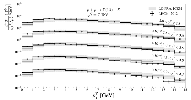
Figure 1: Prompt $\Upsilon(1S)$ production cross section as a function of transverse momenta at the $\sqrt{s}=7$ TeV at the different ranges of rapidity. The data are from LHCb Collaboration Aaij et al. (2015).

Figure 2: Prompt $J/\psi$ production cross section as a function of transverse momenta at the $\sqrt{s}=7$ TeV at the different ranges of rapidity. The data are from LHCb Collaboration Aaij et al. (2011).

In the DPS scenario, the cross section for the associated production of a quarkonium $\mathcal{Q}$ and $D-$meson is expressed in terms of the cross sections of two independent subprocesses

$$\sigma^{\rm DPS}(p+p\to\mathcal{Q}+D+X)=\frac{\sigma^{\rm SPS}(p+p\to\mathcal{Q}+X_{1})\times\sigma^{\rm SPS}(p+p\to D+X_{2})}{\sigma_{\rm eff}},$$ (8)

where parameter $\sigma_{\rm eff}$ controls the contribution of the DPS mechanism. To calculate $J/\psi+D$ and $\Upsilon+D$ associated productions we take here parameters ${\cal F}^{\psi}\simeq{\cal F}^{\Upsilon}=0.02$ as it was early obtained by the fit of the LHCb data for the single prompt $J/\psi$ production cross section  Chernyshev and Saleev (2022) and single prompt $\Upsilon$ production Saleev and Chernyshev (2023) using the ICEM and event generator KaTie. The DPS parameter is taken equal $\sigma_{\rm eff}=11$ mb as it follows from the fit of $J/\psi$ and $\Upsilon$ pair production cross sections and spectra using the same approaches Chernyshev and Saleev (2022); Saleev and Chernyshev (2023).

In the Figs. 1 and 2, we plot theoretical predictions for transverse momentum spectra $(p_{T})$ of prompt $\Upsilon$ and $J/\psi$ obtained within the ICEM and $k_{T}-$factorization using generator KaTie van Hameren (2018) and modified uPDFs Nefedov and Saleev (2020). The good agreement with the LHCb data Aaij et al. (2015, 2011) at the $\sqrt{s}=7$ is founded. The shadow bounds demonstrate theoretical uncertainty following from the choice of the hard scale $\mu$, which is taken as $\mu=\xi\sqrt{M_{Q}^{2}+p_{T}^{2}}$ with $\xi=\frac{1}{2},~{}1,~{}2$.

IV Fragmentation approach

For description of the inclusive production of an open charm meson it is often used the fragmentation approach in which the cross section for the production of $D-$meson is related to the $c\bar{c}$ pair production by the following way:

$$\frac{d\sigma^{\rm SPS}(p+p\to D+X)}{d^{2}p_{TD}dy_{D}}=\int\limits_{z_{\rm cut}}^{1}dz\ {\cal D}_{c\to D}(z)\ \frac{d\sigma^{\rm SPS}(p+p\to c+\bar{c}+X)}{d^{2}p_{Tc}dy_{c}},$$ (9)

where ${\cal D}_{c\to D}(z)$ is a fragmentation function (FF) of the $c-$quark into $D-$meson, $p_{c}$ is $c-$quark 4-momentum expressed in terms of $D-$meson 4-momentum $p_{D}$ through parameter $z$, which is defined as

$$z=\frac{E_{D}+|{\bf p}_{D}|}{E_{c}+|{\bf p}_{c}|}.$$

The minimal value of parameter $z_{\rm cut}=m_{D}/(E_{c}+|{\bf p}_{c}|)$ cuts out the non-physical region, where $E_{c}<m_{D}$, and we apply collinear fragmentation approximation, ${{\bf p}_{D}}/{|{\bf p}_{D}|}={{\bf p}_{c}}/{|{\bf p}_{c}|}$. In our calculations, we use so-called Peterson FF

$${\cal D}_{c\to D}(z)={\cal N}\ \frac{z\ (1-z)^{2}}{[(1-z)^{2}+\epsilon\,z]^{2}}$$ (10)

with parameter $\epsilon=0.06$. FF is normalized such that

$$\int_{0}^{1}dz\ {\cal D}_{c\to D}(z)=P_{c\to D},$$ (11)

where $P_{c\to D^{+}}=0.225$ and $P_{c\to D^{0}}=0.542$. Gladilin (1999).

To test fragmentation approach, we performed calculations for $D^{+,0}-$meson transverse momentum spectra and compare obtained results with the relevant LHCb data Aaij et al. (2013) at the energy $\sqrt{s}=7$ TeV, as it is shown in the Figs. 3 and 4.

Such a way, we demonstrate applicability of our approach based on the $k_{T}-$factorization with the modified KMRW unPDFs, the ICEM and the fragmentation model, for description of single heavy quarkonium and single D-meson production. Now, we are in position to study associated $J/\psi(\Upsilon)+D$ production.

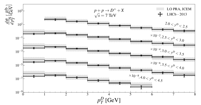
Figure 3: $D^{+}$-meson production cross sections as functions of transverse momenta at the $\sqrt{s}=7$ TeV. The data are from the LHCb Collaboration Aaij et al. (2013).

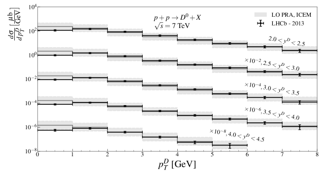
Figure 4: $D^{0}$-meson production cross sections as functions of transverse momenta at the $\sqrt{s}=7$ TeV. The data are from the LHCb Collaboration Aaij et al. (2013).

V Associated $J/\psi(\Upsilon)+D$ production

In case of $J/\psi+D$ associated production via the SPS, we take into account contributions of the following parton subprocesses:

$$R+R \to c+\bar{c}+c+\bar{c},$$ (12)

$$Q_{q}+\bar{Q}_{q} \to c+\bar{c}+c+\bar{c},$$ (13)

where $R$ is a Reggeized gluon, $Q_{q}(\bar{Q}_{q})$ as a Reggeized quark (antiquark), and $q=u,d,s,c$. In the DPS approach, the processes of the $J/\psi+D$ associated production are following:

$$R+R \to c+\bar{c},$$ (14)

$$Q_{q}+\bar{Q}_{q} \to c+\bar{c}$$ (15)

in both groups.

In case of $\Upsilon+D$ associated production via the SPS, we take into account contributions of the following parton subprocesses:

$$R+R \to b+\bar{b}+c+\bar{c},$$ (16)

$$Q_{q}+\bar{Q}_{q} \to b+\bar{b}+c+\bar{c}.$$ (17)

In the DPS approach, the processes of $\Upsilon+D$ associated production are following:

$$R+R \to b+\bar{b},$$ (18)

$$Q_{q}+\bar{Q}_{q} \to b+\bar{b}$$ (19)

$$R+R \to c+\bar{c},$$ (20)

$$Q_{q}+\bar{Q}_{q} \to c+\bar{c}.$$ (21)

Using the KaTie, we can do calculations up to four particles in a final state that it is enough for our purposes. We put masses of quarks, heavy mesons and heavy quarkonia during the calculations equal $m_{c}=1.3$ GeV, $m_{b}=4.5$ GeV, $m_{D^{+}}=1.87$ GeV, $m_{D^{0}}=1.86$ GeV, $m_{B^{+}}=5.28$ GeV, $m_{J/\psi}=3.097$ GeV, $m_{\Upsilon}=9.46$ GeV. As it was already mentioned in the Section II, we use modified KMRW uPDFs Nefedov and Saleev (2020), which were used previously in our calculations for $J/\psi(\Upsilon)$ pair production using event generator KaTie Chernyshev and Saleev (2022); Saleev and Chernyshev (2023).

The results of our calculations for associated $J/\psi+D^{+,0}$ production are presented in the Figs. 5 and 6 and for associated $\Upsilon+D^{+,0}$ production in the Figs. 7 and 8. We have obtained quite satisfactory agreement between data and our calculations for all spectra in $J/\psi+D$ and $\Upsilon+D$ associated production. There are disagreements only in the rapidity difference spectra, especially in $J/\psi+D$ production, at the large values of $|\Delta y^{\psi D}|$. We find theoretical calculations overestimate LHCb data at the $|\Delta y^{\psi D}|\simeq 1.75-2.0$ about one order of magnitude.

In the Table 1 we collect our theoretical predictions for associated ${J/\psi(\Upsilon)+D}$ production cross sections at the $\sqrt{s}=7,8$ TeV and $\sqrt{s}=13$ TeV. The predictions at the $\sqrt{s}=7,8$ TeV are compared with the experimental data. We find a quite good agreement between data and theoretical calculations, which correspond the default choice of the hard scale $\mu=\frac{1}{2}\left(m^{\cal Q}_{T}+m^{D}_{T}\right)$, where $m^{\cal Q}_{T}=\sqrt{m_{\cal Q}^{2}+p_{T,{\cal Q}}^{2}}$ and $m^{D}_{T}=\sqrt{m_{D}^{2}+p_{T,{D}}^{2}}$. The variation of hard scale by factor 2 around the default value gives an estimation of uncertainty of $k_{T}-$factorization calculation. In case of the DPS production, such uncertainty may be very large, about 100 % at the up limit, instead off the SPS production mechanism. It is due to we have the product of four uPDFs in the DPS calculation, each of them sufficiently depend on the choice of hard scale $\mu$.

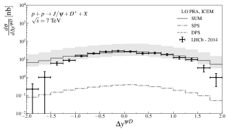
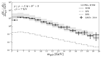
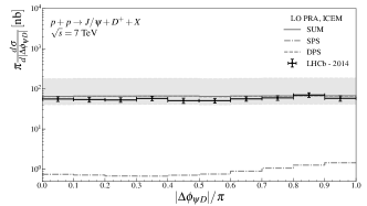
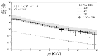
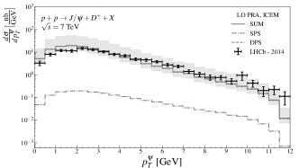
Figure 5: Various spectra for associated $J/\psi+D^{+}$ production at the $\sqrt{s}=7$ TeV: $\Delta y^{\psi D}$ - rapidity difference, $m^{\psi D}$ - invariant mass, $|\Delta\phi^{\psi D}|$ - azimuthal angle difference, $p_{T}^{D}$ - $D^{+}$ transverse momentum and $p_{T}^{\psi}$ - $J/\psi$ transverse momentum. The dashed line is the DPS contribution, the dashed-dotted line is the SPS contribution, solid line is they sum. Grey bounds around the solid line are scale uncertainties of calculations. The data are from LHCb collaboration Aaij et al. (2012).

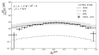
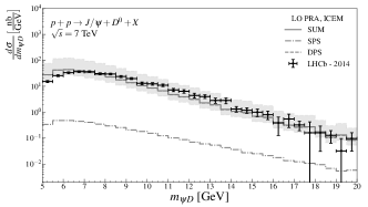
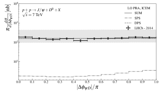
Figure 6: Various spectra for associated $J/\psi+D^{0}$ production at the $\sqrt{s}=7$ TeV: $\Delta y^{\psi D}$ - rapidity difference, $m^{\psi D}$ - invariant mass, $|\Delta\phi^{\psi D}|$ - azimuthal angle difference, $p_{T}^{D}$ - $D^{0}$ transverse momentum and $p_{T}^{\psi}$ - $J/\psi$ transverse momentum. The dashed line is the DPS contribution, the dashed-dotted line is the SPS contribution, solid line is they sum. Grey bounds around the solid line are scale uncertainties of calculations. The data are from LHCb collaboration Aaij et al. (2012) .

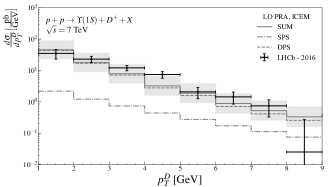
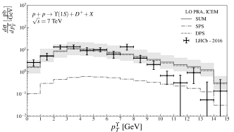
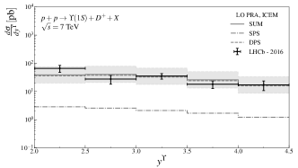
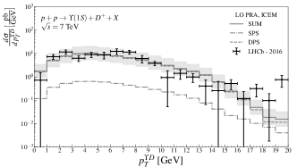
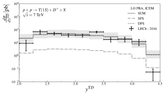
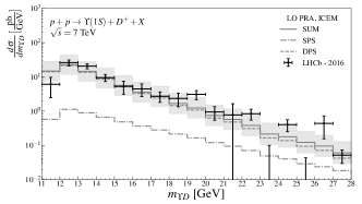
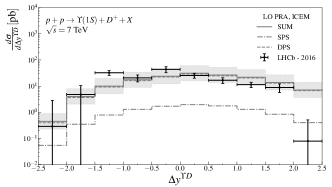
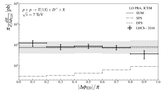
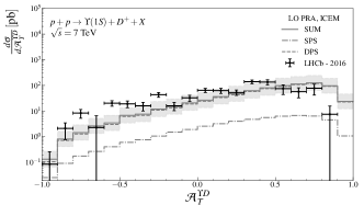
Figure 7: Various spectra for associated $\Upsilon+D^{+}$ production at the $\sqrt{s}=7$ TeV: $y^{\Upsilon}$ - $\Upsilon$ rapidity, $y^{D}$ - $D^{+}$ rapidity, $|\Delta y_{\Upsilon D}|$ - rapidity difference, $m_{\Upsilon D}$ - invariant mass, $|\Delta\phi_{\Upsilon D}|$ - azimuthal angle difference, $p_{T}^{D}$ - $D^{+}$ transverse momentum, $p_{T}^{\Upsilon}$ - $\Upsilon$ transverse momentum, $p_{T}^{\Upsilon D}$ - $\Upsilon+D^{+}$ transverse momentum, $A_{T}^{\Upsilon D}$ - transverse momentum difference. The dashed line is the DPS contribution, the dashed-dotted line is the SPS contribution. Grey bounds around the solid line are scale uncertainties of calculations. The data are from LHCb collaboration Aaij et al. (2016).

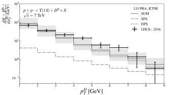
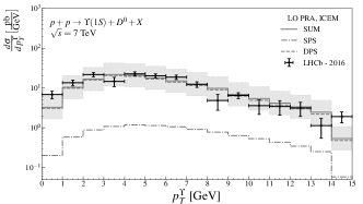
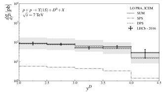
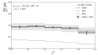
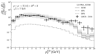
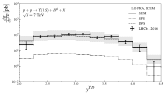
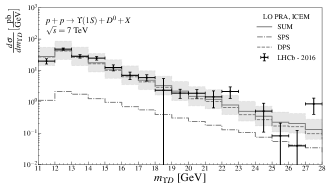
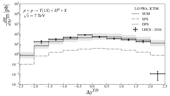
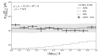
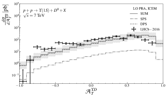
Figure 8: Various spectra for associated $\Upsilon+D^{0}$ production at the $\sqrt{s}=7$ TeV: $y^{\Upsilon}$ - $\Upsilon$ rapidity, $y^{D}$ - $D^{0}$ rapidity, $|\Delta y^{\Upsilon D}|$ - rapidity difference, $m_{\Upsilon D}$ - invariant mass, $|\Delta\phi_{\Upsilon D}|$ - azimuthal angle difference, $p_{T}^{D}$ - $D^{+}$ transverse momentum, $p_{T}^{\Upsilon}$ - $\Upsilon$ transverse momentum, $p_{T}^{\Upsilon D}$ - $\Upsilon+D^{0}$ transverse momentum, $A_{T}^{\Upsilon D}$ - transverse momentum difference. The dashed line is the DPS contribution, the dashed-dotted line is the SPS contribution, solid line is they sum. Grey bounds around the solid line are scale uncertainties of calculations. The data are from LHCb collaboration Aaij et al. (2016).

Final state	Energy	Cross section	Experiment $\pm\,(\rm stat)\pm(\rm syst)$	KaTie $\pm\,\Delta_{\rm SPS}\pm\Delta_{\rm DPS}$
$J/\psi+D^{0}$	$\sqrt{s}=7$ TeV	${\cal B}(J/\psi\to\mu^{+}\mu^{-})\times\sigma$	$9.7\pm 0.2\pm 0.7\ [\rm nb]$	$9.6\ {}^{+0.4}_{-0.1}\ {}^{+26.1}_{-5.9}\ [\rm nb]$
$J/\psi+D^{+}$	$\sqrt{s}=7$ TeV	${\cal B}(J/\psi\to\mu^{+}\mu^{-})\times\sigma$	$3.4\pm 0.1\pm 0.4\ [\rm nb]$	$3.9\ {}^{+0.2}_{-0.02}\ {}^{+10.8}_{-2.4}\ [\rm nb]$
$\Upsilon+D^{0}$	$\sqrt{s}=7$ TeV	${\cal B}(\Upsilon\to\mu^{+}\mu^{-})\times\sigma$	$155\pm 21\pm 7\ [\rm pb]$	$145\ {}^{+16}_{-6}\ {}^{+124}_{-65}\ [\rm pb]$
$\Upsilon+D^{+}$	$\sqrt{s}=7$ TeV	${\cal B}(\Upsilon\to\mu^{+}\mu^{-})\times\sigma$	$82\pm 19\pm 5\ [\rm pb]$	$78\ {}^{+14}_{-2}\ {}^{+140}_{-38}\ [\rm pb]$
$\Upsilon+D^{0}$	$\sqrt{s}=8$ TeV	${\cal B}(\Upsilon\to\mu^{+}\mu^{-})\times\sigma$	$250\pm 28\pm 11\ [\rm pb]$	$255\ {}^{+25}_{-9}\ {}^{+189}_{-113}\ [\rm pb]$
$\Upsilon+D^{+}$	$\sqrt{s}=8$ TeV	${\cal B}(\Upsilon\to\mu^{+}\mu^{-})\times\sigma$	$80\pm 16\pm 5\ [\rm pb]$	$85\ {}^{+8}_{-3}\ {}^{+63}_{-37}\ [\rm pb]$
Predictions
$J/\psi+D^{0}$	$\sqrt{s}=13$ TeV	${\cal B}(J/\psi\to\mu^{+}\mu^{-})\times\sigma$	$-$	$34.3\ {}^{+0.5}_{-0.2}\ {}^{+36.9}_{-17.6}\ [\rm nb]$
$J/\psi+D^{+}$	$\sqrt{s}=13$ TeV	${\cal B}(J/\psi\to\mu^{+}\mu^{-})\times\sigma$	$-$	$14.2\ {}^{+0.2}_{-0.1}\ {}^{+15.3}_{-7.3}\ [\rm nb]$
$\Upsilon+D^{0}$	$\sqrt{s}=13$ TeV	${\cal B}(\Upsilon\to\mu^{+}\mu^{-})\times\sigma$	$-$	$475\ {}^{+31}_{-12}\ {}^{+344}_{-210}\ [\rm pb]$
$\Upsilon+D^{+}$	$\sqrt{s}=13$ TeV	${\cal B}(\Upsilon\to\mu^{+}\mu^{-})\times\sigma$	$-$	$197\ {}^{+13}_{-5}\ {}^{+143}_{-82}\ [\rm pb]$

Table 1: Comparison of theoretical and experimental total cross sections for associated $J/\psi(\Upsilon)+D^{+,0}$ production. The theoretical uncertainties include the variation of the hard scale by factors $\xi=2$, and $\frac{1}{2}$ from it’s default value $\mu=\frac{1}{2}\left(m^{\cal Q}_{T}+m^{D}_{T}\right)$.

VI Conclusions

Working in the ICEM and the $k_{T}-$factorization, taking into account the SPS and the DPS mechanisms, we have obtained self agreement description of the LHCb data for prompt heavy quarkonium $(J/\psi,\Upsilon)$ production, inclusive $D^{+,0}-$meson production, heavy quarkonium pair production $(J/\psi J/\psi,\Upsilon\Upsilon,J/\psi\Upsilon)$ Chernyshev and Saleev (2022); Saleev and Chernyshev (2023) and heavy quarkonium plus $D^{+,0}-$meson associated production in the high-energy proton-proton collisions. In this study, we confirm early obtained numerical values for parameters of the ICEM, $F^{\psi}\simeq F^{\Upsilon}\simeq 0.02$, and the DPS pocket formula, $\sigma_{eff}\simeq 11$ mb, which don’t contradict results obtained previously by the different studies within the ICEM, the $k_{T}-$factorization and the DPS model. It is shown that the $k_{T}-$factorization, which involves into consideration high-order QCD corrections included in uPDFs, may be a powerful tool to calculate multi-particle production cross sections and spectra in the multi-Regge kinematics. The efficiency of event generator KaTie for calculations in the $k_{T}-$factorization approach is demonstrated once more.

References

- Aaij et al. (2012) R. Aaij et al. (LHCb), JHEP 06, 141 (2012), [Addendum: JHEP 03, 108 (2014)], eprint 1205.0975.
- Aaij et al. (2016) R. Aaij et al. (LHCb), JHEP 07, 052 (2016), eprint 1510.05949.
- Calucci and Treleani (1999) G. Calucci and D. Treleani, Phys. Rev. D 60, 054023 (1999), eprint hep-ph/9902479.
- Chapon et al. (2022) E. Chapon et al., Prog. Part. Nucl. Phys. 122, 103906 (2022), eprint 2012.14161.
- Baier and Ruckl (1983) R. Baier and R. Ruckl, Z. Phys. C 19, 251 (1983).
- Berger and Jones (1981) E. L. Berger and D. L. Jones, Phys. Rev. D 23, 1521 (1981).
- Bodwin et al. (1995) G. T. Bodwin, E. Braaten, and G. P. Lepage, Phys. Rev. D 51, 1125 (1995), [Erratum: Phys.Rev.D 55, 5853 (1997)], eprint hep-ph/9407339.
- Shao (2020) H.-S. Shao, Phys. Rev. D 102, 034023 (2020), eprint 2005.12967.
- Berezhnoy and Likhoded (2015) A. V. Berezhnoy and A. K. Likhoded, Int. J. Mod. Phys. A 30, 1550125 (2015), eprint 1503.04445.
- Likhoded et al. (2016) A. Likhoded, A. Luchinsky, and S. Poslavsky, Phys. Lett. B 755, 24 (2016), eprint 1511.04851.
- Karpishkov et al. (2019) A. V. Karpishkov, M. A. Nefedov, and V. A. Saleev, Phys. Rev. D 99, 096021 (2019), eprint 1904.05004.
- Collins and Ellis (1991) J. C. Collins and R. K. Ellis, Nucl. Phys. B 360, 3 (1991).
- Catani and Hautmann (1994) S. Catani and F. Hautmann, Nucl. Phys. B 427, 475 (1994), eprint hep-ph/9405388.
- Gribov et al. (1983) L. V. Gribov, E. M. Levin, and M. G. Ryskin, Phys. Rept. 100, 1 (1983).
- Aaij et al. (2023a) R. Aaij et al. (LHCb) (2023a), eprint 2305.15580.
- Aaij et al. (2023b) R. Aaij et al. (LHCb) (2023b), eprint 2311.14085.
- Ma and Vogt (2016) Y.-Q. Ma and R. Vogt, Phys. Rev. D 94, 114029 (2016), eprint 1609.06042.
- Cheung and Vogt (2017) V. Cheung and R. Vogt, Phys. Rev. D 95, 074021 (2017), eprint 1702.07809.
- Cheung and Vogt (2021) V. Cheung and R. Vogt, Phys. Rev. D 104, 094026 (2021), eprint 2102.09118.
- Cheung and Vogt (2018) V. Cheung and R. Vogt, Phys. Rev. D 98, 114029 (2018), eprint 1808.02909.
- Maciuła et al. (2019) R. Maciuła, A. Szczurek, and A. Cisek, Phys. Rev. D 99, 054014 (2019), eprint 1810.08063.
- Chernyshev and Saleev (2022) A. A. Chernyshev and V. A. Saleev, Phys. Rev. D 106, 114006 (2022), eprint 2211.07989.
- Saleev and Chernyshev (2023) V. A. Saleev and A. A. Chernyshev, Phys. Part. Nucl. Lett. 20, 389 (2023).
- Maciuła et al. (2016) R. Maciuła, V. A. Saleev, A. V. Shipilova, and A. Szczurek, Phys. Lett. B 758, 458 (2016), eprint 1601.06981.
- van Hameren et al. (2015) A. van Hameren, R. Maciuła, and A. Szczurek, Phys. Lett. B 748, 167 (2015), eprint 1504.06490.
- van Hameren (2018) A. van Hameren, Comput. Phys. Commun. 224, 371 (2018), eprint 1611.00680.
- Karpishkov et al. (2017) A. V. Karpishkov, M. A. Nefedov, and V. A. Saleev, Phys. Rev. D 96, 096019 (2017), eprint 1707.04068.
- Nefedov and Saleev (2020) M. A. Nefedov and V. A. Saleev, Phys. Rev. D 102, 114018 (2020), eprint 2009.13188.
- Kimber et al. (2001) M. A. Kimber, A. D. Martin, and M. G. Ryskin, Phys. Rev. D 63, 114027 (2001), eprint hep-ph/0101348.
- Watt et al. (2003) G. Watt, A. D. Martin, and M. G. Ryskin, Eur. Phys. J. C 31, 73 (2003), eprint hep-ph/0306169.
- van Hameren et al. (2013a) A. van Hameren, P. Kotko, and K. Kutak, JHEP 01, 078 (2013a), eprint 1211.0961.
- van Hameren et al. (2013b) A. van Hameren, K. Kutak, and T. Salwa, Phys. Lett. B 727, 226 (2013b), eprint 1308.2861.
- Nefedov et al. (2013) M. A. Nefedov, V. A. Saleev, and A. V. Shipilova, Phys. Rev. D 87, 094030 (2013), eprint 1304.3549.
- Kutak et al. (2016) K. Kutak, R. Maciula, M. Serino, A. Szczurek, and A. van Hameren, JHEP 04, 175 (2016), eprint 1602.06814.
- Lipatov (1995) L. N. Lipatov, Nucl. Phys. B 452, 369 (1995), eprint hep-ph/9502308.
- Lipatov and Vyazovsky (2001) L. N. Lipatov and M. I. Vyazovsky, Nucl. Phys. B 597, 399 (2001), eprint hep-ph/0009340.
- Aaij et al. (2015) R. Aaij et al. (LHCb), JHEP 11, 103 (2015), eprint 1509.02372.
- Aaij et al. (2011) R. Aaij et al. (LHCb), Eur. Phys. J. C 71, 1645 (2011), eprint 1103.0423.
- Gladilin (1999) L. K. Gladilin (H1, ZEUS), Nucl. Phys. B Proc. Suppl. 75, 117 (1999).
- Aaij et al. (2013) R. Aaij et al. (LHCb), Nucl. Phys. B 871, 1 (2013), eprint 1302.2864.