Class Information Guided Reconstruction for Automatic Modulation Open-Set Recognition

Abstract

Automatic Modulation Recognition (AMR) is a crucial technology in the domains of radar and communications. Traditional AMR approaches assume a closed-set scenario, where unknown samples are forcibly misclassified into known classes, leading to serious consequences for situation awareness and threat assessment. To address this issue, Automatic Modulation Open-set Recognition (AMOSR) defines two tasks as Known Class Classification (KCC) and Unknown Class Identification (UCI). However, AMOSR faces core challenges in terms of inappropriate decision boundaries and sparse feature distributions. To overcome the aforementioned challenges, we propose a Class Information guided Reconstruction (CIR) framework, which leverages reconstruction losses to distinguish known and unknown classes. To enhance distinguishability, we design Class Conditional Vectors (CCVs) to match the latent representations extracted from input samples, achieving perfect reconstruction for known samples while yielding poor results for unknown ones. We also propose a Mutual Information (MI) loss function to ensure reliable matching, with upper and lower bounds of MI derived for tractable optimization and mathematical proofs provided. The mutually beneficial CCVs and MI facilitate the CIR attaining optimal UCI performance without compromising KCC accuracy, especially in scenarios with a higher proportion of unknown classes. Additionally, a denoising module is introduced before reconstruction, enabling the CIR to achieve a significant performance improvement at low SNRs. Experimental results on simulated and measured signals validate the effectiveness and the robustness of the proposed method.

I Introduction

Automatic Modulation Recognition (AMR) pertains to the classification of intra-pulse modulation types, which has a wide range of applications in military and civilian fields [1, 2]. Within military applications, AMR aids the inference of radar intentions, facilitates effective radar operation and contributes to further specific emitter identification [3, 4]. For civilian use, AMR provides modulation details necessary for spectrum management [5, 6] and monitors the spectrum to prevent malicious attacks. These capabilities of AMR make it an essential technology for enabling dynamic spectrum access and ensuring physical-layer security for Internet of Things (IoT) networks [7, 8, 9].

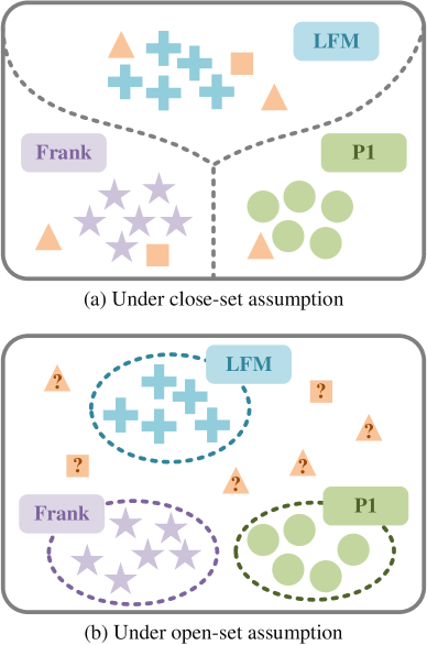
Figure 1: Comparison of closed-set and open-set assumptions. Under close-set assumption, samples from unknown classes are forcibly misclassified to one of known classes. Under open-set assumption, the unknown modulation types are assigned to a distinct category denoted as the unknown class.

As the development of Deep Learning (DL), many DL-based AMR approaches have been proposed [10, 11, 12, 13, 14, 15, 16, 17]. Under a closed-set assumption, wherein the modulation types in the training and test sets are identical, these methods have demonstrated promising performance. However, the closed-set paradigm poses limitations for real-world electromagnetic environments, wherein signals with unknown modulation types not seen during training are likely to be encountered [18]. Under a closed-set assumption, such unknown modulation types would be forcibly assigned to one of the known classes during prediction, as shown in Fig. 1 (a). This mis-classification can lead to inaccurate situation awareness by perceiving unknown threats as familiar ones. Additionally, defensive techniques may no longer be optimally matched to adversary systems whose types were not precisely determined.

To mitigate the issue of mis-classification, Automatic Modulation Open-Set Recognition (AMOSR) is introduced, wherein the test set may contain modulation types that are not encountered during training [19, 20, 21, 22]. Specifically, when encountering unknown modulation types during testing, we explicitly assign them to a distinct category denoted as the unknown class, instead of erroneously labeling them as an existing class, as presented in Fig. 1 (b). The AMOSR formulates two objectives: Known Class Classification (KCC) and Unknown Class Identification (UCI), which is better aligned with real-world electromagnetic environments. However, existing AMOSR approaches face two key challenges in accomplishing these objectives: (1) Inappropriate decision boundary; (2) Sparse feature distribution.

The first challenge in AMOSR is inappropriate decision boundary, which usually stems from incompatible assumptions. Specifically, certain methods relied on the assumption that certain samples were naturally distorted versions of their classes [23, 24, 25] and could be utilized to delineate the decision boundary. However, when extending this assumption directly to AMOSR, a significant number of samples at low SNRs would be incorrectly labeled as unknown. This is because distortions in signal samples primarily arise from noise contamination, rather than fundamentally altering the modulation-specific time-frequency signatures.

The second challenge in AMOSR involves addressing sparse feature distributions exacerbated by noise. Conventional Open-Set Recognition (OSR) techniques aimed to concentrate latent features within single class while increasing margins between classes to attain better OSR performance [26, 27, 28]. However, declining SNR poses unique difficulties for AMOSR. Specifically, at lower SNRs, within-class features become more dispersed as features between classes start to overlap, leading to significant performance degradation. While previous studies investigated OSR tasks on degraded images, such as blurry or noisy photographs, these approaches prove to be ineffective for AMOSR. This is primarily due to the significant corruption and distortion present in Time-Frequency Images (TFI) generated from noise-contaminated received signals.

To tackle the aforementioned challenges, this paper proposes a Class Information guided Reconstruction (CIR) framework for AMOSR. The CIR framework distinguishes known and unknown classes based on reconstruction losses, which provides a reliable metric unaffected by sample deformities and prevent inappropriate decision boundary. To enhance the discriminability of the features used for UCI (i.e. reconstruction losses), the CIR leverages class information by introducing Class Conditional Vectors (CCVs) and Mutual Information (MI) loss function. Perfect reconstruction is achieved only for samples that match the CCVs, while unknown samples that do not match any CCVs yield large reconstruction losses. To ensure the reliability of matching, the framework maximizes the MI between classes and latent representations while minimizing the MI between samples and latent representations for better generalization performance. Furthermore, a denoising module is introduced to mitigate the adverse effects of noise, providing clearer information for subsequent reconstruction stages and ensuring the robustness of CIR at low SNRs.

The main contributions can be summarized as follows:

• We propose a class information guided reconstruction framework for AMOSR that leverages reconstruction losses to jointly accomplish known class classification and unknown class identification.

• Class conditional vectors and mutual information loss function are elaborately designed to significantly enhance the distinguishability of the CIR, attaining optimal UCI performance without compromising KCC accuracy.

• We derive the upper and lower bounds of the mutual information and provide mathematical proofs in detail, enabling tractable optimization of CIR.

• Comprehensive experiments on simulated and measured signals validate the effectiveness and the robustness of the proposed method, especially in scenarios with low SNRs and a higher proportion of unknown classes.

This paper is organized as follows. Section II reviews related OSR methods in Computer Vision (CV) and AMR fields. Section III establishes preliminaries, including signal models, Time-Frequency Analysis (TFA) methods, and problem definition of AMOSR. In Section IV, the proposed CIR is introduced, while the experimental design and the analysis of the results are presented in Section V. Finally, the paper is concluded and future work is discussed in Section VI.

The notations used in this paper are summarized in Table I.

TABLE I: Important Notations

Notations	Definitions
$\bm{\psi}$	Modulation type
$N$	Number of modulation types
$N_{u}$	Number of unknown modulation types
$\mathcal{D}$	Dataset
$\mathcal{L}$	Loss function
$\mathcal{H}$	Fully connected layer
$x_{n}$	Raw TFI
$x$	Denoised TFI
$y$	Class label
$\bm{z}$	Latent representations
$H$	Height of the TFI
$W$	Width of the TFI
$C$	Number of channels
$\bm{F}$	Features in Restormer
$\bm{R}$	Residual image in Restormer
$l$	Class conditional vector
$f$	Frequency
$\gamma$	Lagrange multiplier
$\tau$	Decision threshold
$\sigma$	Weight coefficient

II Related Work

II-A Open-Set Recognition Methods in CV

Discriminative-based approaches: By leveraging the powerful representation learning capability of deep networks, some classical discriminative-based approaches have emerged for OSR task. A plain choice was to utilize the maximum SoftMax probabilities and rejected low-confidence predictions [29]. Bendale et al. [30] proved SoftMax probability was not robust and proposed to replace the SoftMax function with the OpenMax function, which redistributed the scores of SoftMax to obtain the confident score of the unknown class explicitly. In [23], Schlachter et al. proposed to split given data into typical and atypical normal subsets, thus finding a precise boundary to distinguish known classes from unknowns. Yang et al. [27] proposed generalized convolutional prototype learning, which replaced the close-world assumed SoftMax classifier with an open-world oriented prototype model. Chen et al. [26] developed Reciprocal Point Learning (RPL), which performed UCI task based on the otherness with reciprocal points. Subsequently, RPL was further improved to ARPL [28], integrating an extra adversarial training strategy to enhance the model distinguishability by generating confusing training samples.

Generative-based approaches: A number of studies have explored generative-based approaches, wherein Auto-Encoder (AE)-based and reconstruction-based techniques are mainly related to our work. Huang et al. [31] proposed a class-specific semantic reconstruction method, that replaced prototype points with manifolds represented by class-specific AEs and measured class belongingness through reconstruction error. In [32], a Conditional Gaussian Distribution Learning (CGDL) was designed, which utilized Variational Auto-Encoder (VAE) to learn class conditional posterior distributions for OSR tasks. Yoshihashi et al. [33] designed the Classification-Reconstruction learning for OSR (CROSR), which used latent representations for closed set classifier training and unknown detection. In [34], a structured Gaussian mixture VAE was proposed, guaranteeing separable class distributions with known variances in its latent space. Sun et al. [35] designed an AE-based method that learned feature representations by modeling them as mixtures of exponential power distributions. In [36], a VAE contrastive learning method was proposed combined with Pseudo Auxiliary searching strategy to discover a more robust structure.

The preceding discriminative-based and generative-based approaches face significant difficulties as mentioned in Section I. Discriminative-based methods encounter challenges in establishing appropriate decision boundaries in high-dimensional space, leading to the excessive rejection of signals with low SNRs as unknowns. Meanwhile, generative-based approaches struggle to aggregate features, thereby failing to achieve sufficiently promising performance.

II-B Open-Set Recognition Methods in AMR

Machine learning-based approaches: Chakravarthy et al. [37] designed a quantile one-class support vector machine-based algorithm. In [38], isolation forest models were used for each known signal class to perform detection of possible unknown signals. Han et al. [39] proposed a deep class probability output network and gave the confidence of identification results through the Kolmogorov–Smirnov test. While Chen et al. [40] established probability models of known classes based on extreme value theory. In [41], an OSR technology based on Dempster–Shafer evidence theory was proposed.

Deep learning-based approaches: Xu et al. [24] proposed a hybrid OSR approach combining modified Intra-Class Spitting (ICS) method with adversarial samples generation. Subsequently, he  [25] enhanced this via Transformer, attaining more precise boundaries. In [42], an algorithm leveraging vision Transformer, Wasserstein distance and reciprocal points improved OSR efficiency. Gong et al. [43] developed an improved counterfactual GAN architecture with multi-tasking mechanism for signal representation. In [4], Dong et al. proposed a zero-shot learning framework, where signal recognition and reconstruction neural networks were designed to tackle the OSR problem. An OSR model based on transfer deep learning and linear weight decision fusion was designed in [44]. Zhang et al. [45] proposed a modified generalized end-to-end loss to increase the similarity of the same modulation type and reduce the similarity of different types.

The above-mentioned AMOSR methods still face the following problems: (1) some studies directly applied CV-inspired frameworks without adequately addressing key differences in distortion mechanisms between visual and signal data; (2) while some existed work made some improvement by incorporating modulation characteristics, many still relied on relatively simplistic OSR techniques such as ML-based or OpenMax-oriented methods. In a word, further exploration is still needed for AMOSR to address the aforementioned issues.

III Preliminaries

III-A Signal Model

From a receiver’s perspective, signals contaminated with noise can be expressed as:

$$s[k]=x[k]+n[k],0\leq k\leq K$$ (1)

where $x[k]$ represents the noise-free signal, $n[k]$ represents the noise generated due to temperature of transmitter equipment, the receiver part of antenna, etc., $k$ is the sample index, and $K$ is the number of sampling points.

The mathematical expression of $x[k]$ is given as:

$$x[k]=a[k]e^{j\theta[k]}$$ (2)

where $a[k]$ is the non-zero constant envelope (i.e. the amplitude) within the pulse interval $\tau_{pw}$, and usually $a[k]=A$ for $0\leq kT_{s}\leq\tau_{pw}$, where $T_{s}$ is the time interval corresponding to the sampling frequency $f_{s}$. The instantaneous phase $\theta[k]$ can be defined through the instantaneous frequency $f[k]$ and the phase offset $\phi[k]$ as:

$$\theta[k]=2\pi f[k](kT_{s})+\phi[k]$$ (3)

In this work, eleven modulation types are considered: linear frequency modulation (LFM), Costas code, five polyphase codes (Frank, P1, P2, P3 and P4), and four polytime codes (T1, T2, T3 and T4) [46].

III-B Time Frequency Analysis

Time-Frequency Analysis is employed to analyze signal variations in both the time and frequency domains. After TFA, the resulting TFIs can be fed into subsequent networks for feature extraction. The Short-Time Fourier Transform (STFT) is one commonly used technique for TFA.

The STFT involves dividing the signal into multiple short windows and applying the Fourier Transform to each window. By sliding these windows along the time axis, a comprehensive time-frequency representation of the entire signal is obtained as follows

$$\text{STFT}(t,f)=\int_{\infty}^{\infty}x(\delta)h(\delta-t)e^{-j2\pi f\delta}\text{d}\delta$$ (4)

where $h(\delta-t)$ is the window function with the length of $\delta$, $f$ is the frequency.

III-C Problem Definition of AMOSR

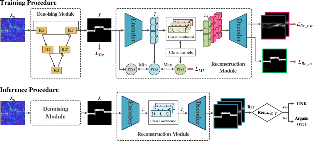
Figure 2: Class information guided reconstruction framework. The proposed CIR consists of two core modules: a denoising module and a reconstruction module. The denoising module receives the raw TFI $x_{n}$ and obtains the denoised TFI $x$. The reconstruction module employs an AE as the backbone, where we propose CCVs and MI loss function to refine the latent representations $\bm{z}$ with class information, effectively increasing the distinguishability. In the inference procedure, the reconstruction losses are utilized to discriminate between known and unknown classes.

Considering $N$ known modulation types, the set of class labels can be denoted as $\bm{\Psi}=\{\psi_{1},\psi_{2},\cdots,\psi_{N}\}$. Given a labeled training set $\mathcal{D}_{\mathcal{L}}=\{(x_{1},y_{1}),(x_{2},y_{2}),\cdots,(x_{n},y_{n})\}$ where labels $y_{i}\in\bm{\Psi}$, and a test set $\mathcal{D}_{\mathcal{T}}=\{t_{1},t_{2},\cdots,t_{u}\}$ where the label of $t_{j}$ belongs to $\bm{\Psi}\cup\{\psi_{N+1},\psi_{N+2},\cdots,\psi_{N+N_{u}}\}$, where $N_{u}$ is the number of unknown classes that would be encountered in realistic scenarios. AMOSR can be divided into two sub-tasks: KCC and UCI. The goal of KCC is to learn a model from $\mathcal{D}_{\mathcal{L}}$ that can accurately predict class labels for test samples whose true labels are contained within $\bm{\Psi}$. The goal of UCI is to have the model assign a unified unknown label $\psi_{N+1}$ to samples whose true labels belong to $\{\psi_{N+1},\psi_{N+2},\cdots,\psi_{N+N_{u}}\}$.

IV Method

IV-A Overall Framework

The proposed CIR utilizes reconstruction losses to distinguish known and unknown classes, which consists of two core modules: a denoising module and a reconstruction module, as presented in Fig. 2. The denoising module is introduced before reconstruction to ensure its functionality at low SNRs. Restormer is utilized as the backbone to denoise the raw input TFI $x_{n}$ and obtain noise-reduced signal $x$. The reconstruction module employs an AE structure to reconstruct the denoised signal $x$, where the CCVs and MI loss function are elaborately designed to enlarge the reconstruction discrepancy between known-class and unknown-class samples. In the training procedure, only latent representations $\bm{z}$ extracted from $x$ that match the CCVs can achieve perfect reconstruction, and MI loss function ensures reliable matching.

Since unknown-class samples cannot match any CCVs, their reconstruction losses will be significantly larger than the reconstruction loss for any known-class sample. Therefore, the inference procedure utilizes the difference in reconstruction losses to identify potential unknown classes. Inputs that result in high reconstruction losses can be flagged as an unknown class, while those identified as known classes will be output with their certain labels.

IV-B Denoising Module

Noise is a crucial factor influencing the performance in AMOSR. As the SNR decreases, recognition accuracy severely deteriorates. To improve AMOSR performance under low SNR conditions, the denoising module removes the noise in raw TFIs to make the discriminative information available at subsequent reconstruction stage. This facilitates better boundary setting between known and unknown classes, ensuring the functionality of CIR at low SNRs.

In this paper, Restormer [47] is utilized to realize the denoising module owing to its favorable properties of high efficiency and promising performance. The overall pipeline of the Restormer is presented in Fig. 3. Given a raw input TFI $x_{n}\in{\mathbb{R}}^{H\times W\times 1}$, Restormer first applies a 3x3 convolution to extract initial feature maps $\bm{F}_{0}\in\mathbb{R}^{H\times W\times C}$, where $H\times W$ denotes the spatial dimension and $C$ is the number of channels. These shallow features $\bm{F}_{0}$ are then passed through a 2-level symmetric encoder-decoder and transformed into deep features $\bm{F}_{d}\in\mathbb{R}^{H\times W\times 2C}$. Each level of encoder-decoder contains multiple Restormer blocks, where the number of blocks is gradually increased from the top to bottom levels to maintain efficiency. The encoder hierarchically downsmaples spatially while expanding channels, extracting latent features $\bm{F}_{l}\in\mathbb{R}^{\frac{H}{4}\times\frac{W}{4}\times 4C}$. The decoder takes low-resolution latent features $\bm{F}_{l}$ as input and progressively recovers the high-resolution representations. Pixel unshuffling and shuffling are used for downsampling and upsampling respectively [48]. To assist the recovery process, the encoder features are concatenated with the decoder features via skip connections [49]. Channel reduction is applied via 1x1 convolution at each level. Finally, a convolution layer generates residual image $\bm{R}\in\mathbb{R}^{H\times W\times 1}$, which is added to the degraded input to obtain the restored image: $x=x_{n}+\bm{R}$.

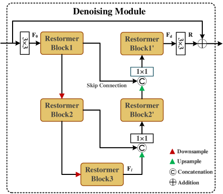
Figure 3: Restormer-based denoising module.

The Restormer block is composed of two core components: (a) multi-Dconv head transposed attention (MDTA) and (b) gated-Dconv feed-forward network (GDFN). These components enable Restormer to achieve highly efficient computation while maintaining strong modeling capabilities. Details of the Restormer block design can be found in [47]. For brevity, the technical details are omitted here as they have been well described in the literature.

The loss function for the denoising module is derived by calculating the Mean Squared Error (MSE) between the denoised TFIs and the ground truth noise-free TFIs as follows:

$$\mathcal{L}_{De}=||x_{n}-x||_{2}^{2}$$ (5)

IV-C Reconstruction Module

The reconstruction module introduces an AE structure to reconstruct the denoised signal $x$, where elaborately designed CCVs and MI loss function refine the latent representations with class information. The CCVs can match the latent representations, achieving perfect reconstruction for known samples and worse reconstruction for unknown samples. Meanwhile, the MI loss function is utilized to ensure reliable matching and improve generalization performance.

As presented in Fig. 2, the encoder maps the input $x$ to low-dimensional latent representations $\bm{z}$. Then, $\bm{z}$ is combined with the designed CCVs to generate the class-conditioned representations $\{\bm{z}_{1},\bm{z}_{2},\cdots,\bm{z}_{N}\}$. Finally, the decoder maps $\{\bm{z}_{1},\bm{z}_{2},\cdots,\bm{z}_{N}\}$ back to the original data space $\{\hat{x}_{1},\hat{x}_{2},\cdots,\hat{x}_{N}\}$, named class-conditioned reconstruction. Meanwhile, the proposed CIR is trained to learn disentangled latent representations by minimizing the MI between the latent representations $\bm{z}$ and the input data $x$, while maximizing the MI between the $\bm{z}$ and the corresponding class labels $y$.

IV-C1 Class-conditioned Reconstruction

The CCVs are designed to match the latent representations, which can help the AE perfectly reconstruct the known-class samples and poorly reconstruct the unknown-class samples, thereby enhancing the discrepancy in reconstruction losses between known-class and unknown-class samples.

Regarding the latent representations $\bm{z}$ obtained from the encoder, the CCV $l_{j}$ is defined as

$$l_{j}(k)=\left\{\begin{aligned} &+1,k=j\\ &-1,k\neq j\end{aligned}\right.\quad k,j\in\{1,2,\cdots,N\}$$ (6)

Then the class-conditioned latent representations $\{\bm{z}_{1},\bm{z}_{2},\cdots,\bm{z}_{N}\}$ are obtained by the following equations,

$$\bm{\alpha}_{j}=\mathcal{H}_{\bm{\alpha}}(l_{j}),\quad\bm{\beta}_{j}=\mathcal{H}_{\bm{\beta}}(l_{j})$$ (7)

$$\bm{z}_{j}=\bm{\alpha}_{j}\odot\bm{z}+\bm{\beta}_{j}$$ (8)

Here, $\mathcal{H}_{\bm{\alpha}}$ and $\mathcal{H}_{\bm{\beta}}$ are fully connected layers, $\bm{\alpha}_{j}$ and $\bm{\beta}_{j}$ have the same shape as vector $\bm{z}$, $\odot$ represents the Hadamard product.

The decoder is expected to perfectly reconstruct the original input when the CCV matches the class identity of the input, referred as the match condition (${\cdot}_{m}$). The perfectly reconstruction is achieved by minimizing the MSE of the reconstructed $\hat{x}_{m}$ and the input $x$. Meanwhile, the decoder is trained to poorly reconstruct the original input when the CCV does not match the class identity of the input, referred as the non-match condition (${\cdot}_{nm}$). The poorly reconstruction is achieved by minimizing the MSE of the reconstructed $\hat{x}_{nm}$ and a randomly sampled signal $x_{r}$ from TFIs not belonging to the current class. The loss function is constructed as follows:

$$\begin{split}&\mathcal{L}_{Re}=\mathcal{L}_{Re\_m}+\mathcal{L}_{Re\_nm}\\ &=\|\hat{x}_{m}-x\|_{2}^{2}+\frac{1}{N-1}\sum_{j=1}^{N-1}\|\hat{x}_{nm}^{j}-x_{r}^{j}\|_{2}^{2}\end{split}$$ (9)

When the input signal belongs to a known class, there exists a CCV that matches the latent representations derived from the input, allowing for near-perfect reconstruction of the input image with minimal reconstruction losses. However, for any input of an unknown class not seen during training, its latent representations cannot be adequately matched with any of the available CCV used for decoding. This mismatch renders the reconstruction ineffective for samples from unknown classes and results in significantly higher reconstruction losses. By leveraging this inherent behavior, the magnitude of reconstruction loss can be utilized to discriminate between known and unknown classes.

IV-C2 Mutual Information Loss Function

The proposed CIR learns to disentangle the latent representations by minimizing the interdependence between the latent representation $\bm{Z}$ and the input $\bm{X}$, while maximizing the correspondence between the $\bm{Z}$ and the respective class labels $\bm{Y}$. In this way, the learned latent representations would contain class-specific information, which allows the latent representations to better match the corresponding CCVs, thereby assisting the role of the class-conditioned reconstruction. Concurrently, it reduces the impact of distribution differences between samples and improves the generalization performance.

The minimizing and maximizing process is achieved by deriving the following objective function [50].

$$\mathcal{L}_{MI}=\text{MI}(\bm{Z},\bm{X})-\gamma\text{MI}(\bm{Z},\bm{Y})$$ (10)

where $\gamma$ is the Lagrange multiplier. $MI(\cdot,\cdot)$ denotes the mutual information with

$$\text{MI}(A,B)=\iint p(a,b)\text{log}\left(\frac{p(a,b)}{p(a)p(b)}\right)\text{d}a\text{d}b$$ (11)

However, directly optimizing Equation 10 is intractable. The MI terms in Equation 10 are thus estimated separately by optimizing the upper bound of $\text{MI}(\bm{Z},\bm{X})$ and the lower bound of $\text{MI}(\bm{Z},\bm{Y})$ as follows:

$$\mathcal{L}_{MI}=\mathcal{L}_{UB}-\gamma\mathcal{L}_{LB}$$ (12)

a) Minimum MI about Input

To learn a latent representation that preserves the minimum MI about the input data, the CIR minimizes the upper bound, and the target objective is written as:

$$\mathcal{L}_{UB}=\mathbb{E}_{p(\bm{Z},\bm{X})}\left[\text{log}p(x|z)\right]-\mathbb{E}_{p(\bm{Z})p(\bm{X})}\left[\text{log}p(x|z)\right]$$ (13)

This paper validates that the upper bound can be estimated through the theoretical analysis, and the theorem format is given as follows:

Theorem 1.

For the random variables $\bm{Z}$ and $\bm{X}$,

$$\text{MI}(\bm{Z},\bm{X})\leq\mathcal{L}_{UB}$$ (14)

Equality is achieved if and only if $\bm{Z}$ and $\bm{X}$ are independent.

Proof.

$$\begin{split}&\qquad\mathcal{L}_{UB}-\text{MI}(\bm{Z},\bm{X})\\ &=\iint p(z,x)\text{log}p(x|z)\text{d}z\text{d}x-\iint p(z)p(x)\text{log}p(x|z)\text{d}x\text{d}z\\ &\quad-\iint p(z,x)\text{log}\left(\frac{p(z,x)}{p(z)p(x)}\right)\text{d}z\text{d}x\\ &=\iint p(z,x)\text{log}p(x)\text{d}z\text{d}x-\iint p(z)p(x)\text{log}p(x|z)\text{d}z\text{d}x\\ &=\int p(x)\text{log}p(x)\text{d}x-\iint p(x)p(z)\text{log}p(x|z)\text{d}x\text{d}z\\ &=\int p(x)\left(\text{log}p(x)-\int p(z)\text{log}p(x|z)\text{d}z\right)\text{d}x\\ \end{split}$$ (15)

By definition, the probability distribution of inputs $x$ can be expressed as $p(x)=\int p(x|z)p(z)\text{d}z$.

Taking the logarithm of both sides yields $\text{log}p(x)=\text{log}\int p(x|z)p(z)\text{d}z$. Applying Jensen’s inequality to the expectation of the logarithm results in:

$$\text{log}\int p(x|z)p(z)\text{d}z\geq\int\text{log}p(x|z)p(z)\text{d}z$$ (16)

Then, the derivation yields the following:

$$\begin{split}&\qquad\mathcal{L}_{UB}-\text{MI}(\bm{Z},\bm{X})\\ &=\int p(x)\text{d}x\left(\text{log}p(x)-\int p(z)\text{log}p(x|z)\text{d}z\right)\\ &\geq\int p(x)\text{d}x\left(\int\text{log}p(x|z)p(z)\text{d}z-\int p(z)\text{log}p(x|z)\text{d}z\right)=0\end{split}$$ (17)

Thus, the upper bound of $MI(\bm{Z},\bm{X})$ is derived. Since $p(x|z)$ is not accessible, A variational approximation distribution $q_{\theta}(x|z)$ is utilized to approximate it. ∎

b) Maximum MI about Class

With the goal of obtaining a representation capturing maximum MI regarding the class label, the lower bound is maximized. This yields the following objective:

$$\mathcal{L}_{LB}=\mathop{sup}\limits_{F_{\phi}}\mathbb{E}_{p(y,z)}[F_{\phi}(y,z)]-\text{log}\left(\mathbb{E}_{p(y)p(z)}[e^{F_{\phi}(y,z)}]\right)$$ (18)

where $F_{\phi}:\mathcal{Y}\times\mathcal{Z}\rightarrow\mathcal{R}$ represents several dense layers.

This paper validates that the lower bound can be estimated through the theoretical analysis, and the theorem format is given as follows:

Theorem 2.

For the random variables $\bm{Z}$ and $\bm{Y}$,

$$\text{MI}(\bm{Z},\bm{Y})\geq\mathcal{L}_{LB}$$ (19)

Equality is achieved if and only if $\bm{Z}$ and $\bm{Y}$ are independent.

Proof.

By definition of MI, the following relationship holds:

$$\text{MI}(\bm{Z},\bm{Y})=\mathcal{D}_{KL}\left(P(\bm{Z},\bm{Y})||P(\bm{Y})P(\bm{Z})\right)$$ (20)

According to the definition of conjugate function estimated by f-divergence, the derivation yields:

$$\begin{split}&\qquad\mathcal{D}_{f}\left(P(\bm{Z},\bm{Y})||P(\bm{Z})P(\bm{Y})\right)\\ &=\iint p(y)p(z)f\left(\frac{p(y,z)}{p(y)p(z)}\right)\text{d}y\text{d}z\\ &=\iint p(y)p(z)\left(\mathop{sup}\limits_{{f^{{}^{\prime}}\in dom(f^{*})}}\left\{\frac{p(y,z)}{p(y)p(z)}f^{{}^{\prime}}-f^{*}(f^{{}^{\prime}})\right\}\right)\text{d}y\text{d}z\\ &\geq\iint p(y)p(z)\left(\frac{p(y,z)}{p(y)p(z)}F(y,z)-f^{*}(F(y,z))\right)\text{d}y\text{d}z\\ &=\iint p(y,z)F(y,z)\text{d}y\text{d}z-\iint p(y)p(z)f^{*}(F(y,z))\text{d}y\text{d}z\end{split}$$ (21)

Then, the KL-divergence can be estimated using $f(y)=y\text{log}y$, deriving the following:

$$\begin{split}&\qquad\mathcal{D}_{KL}\left(P(\bm{Z},\bm{Y})||P(\bm{Z})P(\bm{Y})\right)\\ &=\mathop{sup}\limits_{F:\mathbb{Y}\times\mathbb{Z}\rightarrow\mathbb{R}}\mathbb{E}_{p(y,z)}[F(y,z)]-\text{log}\left(\mathbb{E}_{p(y)p(z)}[e^{F(y,z)}]\right)\\ &\geq\mathop{sup}\limits_{F_{\phi}}\mathbb{E}_{p(y,z)}[F_{\phi}(y,z)]-\text{log}\left(\mathbb{E}_{p(y)p(z)}[e^{F_{\phi}(y,z)}]\right)\\ \end{split}$$ (22)

Thus, the lower bound of $\text{MI}(\bm{Z},\bm{Y})$ is derived. ∎

IV-D Training and Inference Procedure

In the training procedure, the CIR is optimized using a linear combination of the denoising, reconstruction and MI loss:

$$\begin{split}&\mathcal{L}=\sigma(\mathcal{L}_{De}+\mathcal{L}_{Re})+\mathcal{L}_{MI}\\ \end{split}$$ (23)

where $\sigma$ refers to a weight coefficient, and is set to $0.005$ in this case.

The entire inference procedure of the proposed CIR is summarized in Algorithm 1. The raw TFIs $x_{n}$ are fed into the denoising module to obtain noise-reduced TFIs $x$. Then, the encoder in reconstruction module extracts latent representations $\bm{z}$ from $x$, which are combined with the CCVs to produce the class-conditioned representations $\{\bm{z}_{1},\bm{z}_{2},\cdots,\bm{z}_{N}\}$. The decoder subsequently generates the reconstructed TFIs $\{\hat{x}_{1},\hat{x}_{2},\cdots,\hat{x}_{N}\}$. Reconstruction losses are respectively calculated between the inputs and reconstructed outputs. If the minimum reconstruction loss exceeds a predefined threshold $\tau$, the sample is identified as belonging to the unknown class. Alternatively, if the minimum loss is below $\tau$, the sample is classified into the class corresponding to that minimal loss.

Algorithm 1 Inference Algorithm of CIR

1:Well-trained denoising Restormer $\mathcal{N}$, encoder $\mathcal{F}$, decoder $\mathcal{G}$, fully connected layers $\mathcal{H_{\alpha},\mathcal{H_{\beta}}}$

2:Test sample $x_{n}$, CCVs $\{l_{1},\cdots,l_{N}\}$, threshold $\tau$

3:Obtain denoised TFI by Restormer $x=\mathcal{N}(x_{n})$

4:Obtain latent representations by encoder $\bm{z}=\mathcal{F}(x)$

5:for $j=1,\cdots,N$ do

6:     Calculate $\bm{\alpha}_{j}=\mathcal{H}_{\bm{\alpha}}(l_{j})$, $\bm{\beta}_{j}=\mathcal{H}_{\bm{\beta}}(l_{j})$

7:     Obtain the class-conditioned latent representations $\bm{z}_{j}=\bm{\alpha}_{j}\odot\bm{z}+\bm{\beta}_{j}$

8:     Obtain reconstructed TFIs by decoder $\hat{x}_{j}=\mathcal{G}(\bm{z}_{j})$

9:     Calculate the reconstruction loss $Rec(j)=\|x-\hat{x}_{j}\|^{2}_{2}$

10:end for

11:Obtain the predicted label $\hat{y}=\text{argmin}(Rec)$

12:Obtain ${Rec}_{min}=\text{Min}(Rec)$

13:if ${Rec}_{min}\geq\tau$ then

14:     Predict $x_{n}$ as unknown sample with label ${\psi}_{N+1}$

15:else

16:     Predict $x_{n}$ as known sample with label $\hat{y}$

17:end if

V Simulations

V-A Simulation Design

V-A1 Dataset Description

TABLE II: Parameter settings of eleven modulation types

Types	Parameters	Value
All	Carrier frequency	$U(\frac{1}{6},\frac{1}{4})f_{s}$
LFM	Bandwidth	$U(\frac{1}{20},\frac{1}{10})f_{s}$
Costas	Number of frequency hops	$U(3,6)$
	Fundamental frequency	$U(\frac{1}{32},\frac{1}{20})f_{s}$
Frank	Cycles per phase code	$U(4,6)$
	Number of frequency steps	$U(4,6)$
P1, P2	Cycles per phase code	$U(4,6)$
	Number of frequency steps	$U(4,6)$
P3, P4	Cycles per phase code	$U(4,6)$
	Number of sub-codes	$\{16,25,36\}$
T1, T2	Number of phase states	$U(2,3)$
	Number of segments	$U(4,6)$
T3, T4	Number of phase states	$U(2,3)$
	Bandwidth	$U(\frac{1}{20},\frac{1}{10})f_{s}$

• U(a,b) represents uniform sampling.

This study considers 11 modulation types as described in Section III, with their parameter settings presented in Table II. The sampling frequency $f_{s}$ is set to 50MHz. The carrier frequency $f_{c}$ is randomly sampled within $(\frac{1}{6},\frac{1}{4})f_{s}$ and the pulse width is $6\mu s$. The additional white Gaussian noise (AWGN) is considered to simulate real-world conditions, where the SNRs are varied from $-$10 to 10 dB with 2dB increments. TFA is conducted on each waveform sample, resulting in a TFI with size of $300\times 256$, and the TFIs are subsequently downsampled to a smaller size of $80\times 80$. Each modulation type consists of 500 signal samples at each SNR level. These samples are split into training and test datasets in a 4:1 ratio.

For AMOSR problems, the test dataset contains unknown class samples that are not present in the training dataset. Therefore, we need to select specific modulation types as unknown classes to partition the training and test datasets. Depending on the specific experimental objectives, we split the dataset as presented in Table III. Dataset D1 is designed to assess the performance of CIR when different modulation types are treated as unknown classes. Dataset D2 is constructed to validate the performance of CIR across varying levels of openness. Openness is utilized to measure the ratio of known classes and unknown classes, defined as

$$\text{Openness}=1-\sqrt{\frac{N}{N+N_{u}}}$$ (24)

As the number of unknown modulation types increases, the degree of openness increases. Lastly, dataset D3 focuses on evaluating the robustness of CIR against different SNRs.

TABLE III: Dataset Configuration

Datasets	SNR	Training Datasets	Testing Datasets (UNK)
D1	[-10,-6,-2]dB	LFM\Costas\Frank\P3\P4\T2\T4	P1\P2\T1\T3
		Frank\P1\P2\T1$-$T4	LFM\Costas\P3\P4
		LFM\ P1$-$P4\T1\T3	Frank\Costas\T2\T4
		LFM\Costas\Frank\P1\P2\T1\T3	P3\P4\T2\T4
D2	[-8,-4,0,4]dB	LFM\Costas\Frank\P2$-$P4\T1$-$T4	P1
		LFM\Costas\Frank\P3\P4\T1$-$T4	P1\P2
		LFM\Costas\Frank\P3\P4\T2$-$T4	P1\P2\T1
		LFM\Costas\Frank\P3\P4\T2\T4	P1\P2\T1\T3
		LFM\ Frank\P3\P4\T2\T4	Costas\P1\P2\T1\T3
		LFM\P3\P4\T2\T4	Costas\Frank\P1\P2\T1\T3
		LFM\P4\T2\T4	Costas\Frank\P1$-$P3\T1\T3
		LFM\T2\T4	Costas\Frank\P1$-$P4\T1\T3
		LFM\T4	Costas\Frank\P1$-$P4\T1$-$T3
		LFM	Costas\Frank\P1$-$P4\T1$-$T4
D3	[-10,-8-6,-4,-2, 2,4,6,8,10]dB	LFM\P1$-$P4\T1\T3	Frank\Costas\T2\T4

V-A2 Baseline Method

In this paper, we selected two discriminative-based and two generative-based OSR methods as baseline methods. They are described as follows:

• Openmax: OpenMax involves training a classifier to recognize known categories, computing the open-set probability for each class, and subsequently determining a suitable threshold to identify unknown categories.[30].

• RPL: Reciprocal Points Learning introduces reciprocal points as the potential representation of the extra-class space corresponding to each known class, optimizing a better feature space to separate known and unknown.[26].

• CGDL: Conditional Gaussian Distribution Learning is a method that utilizes VAE to learn class conditional posterior distributions for unknown detection [32].

• CROSR: Classification-Reconstruction learning for Open-Set Recognition trains networks for joint classification and reconstruction and utilizes latent representations for unknown detection [33].

To ensure a fair comparison, we confirm that the parameters of the above baseline methods are fine-tuned at their best state for the experimental dataset.

V-A3 Evaluation Metrics

a) Metrics for KKC

The recognition accuracy of known samples (AKS) can be defined as:

$$\text{AKS}=\frac{\sum_{i=1}^{N}(\text{TP}_{i}+\text{TN}_{i})}{\sum_{i=1}^{N}(\text{TP}_{i}+\text{TN}_{i}+\text{FP}_{i}+\text{FN}_{i})}$$ (25)

where $N$ represents the number of known classes. TP_i and FP_i represent the number of correctly and incorrectly classified positive samples of the $i$-th class, respectively. TN_i and FN_i represent the number of correctly and incorrectly classified negative samples of the $i$-th class, respectively.

b) Metrics for UCI

The rejection accuracy of unknown samples (AUS) can be defined as:

$$\text{AUS}=\frac{\text{TU}}{\text{TU}+\text{FU}}$$ (26)

where TU represents the number of correctly identified unknown samples, while FU represents the number of incorrectly identified unknown samples.

The area under ROC curve (AUROC) can be defined as:

$$\text{AUROC}=\int_{0}^{1}\text{TPR}\cdot(\text{FPR})^{-1}\text{d}(\text{FPR})$$ (27)

True Positive Rate (TPR) is a metric defined as:

$$\text{TPR}=\frac{\text{TU}}{\text{TU}+\text{FK}}$$ (28)

False Positive Rate (FPR) is a metric defined as:

$$\text{FPR}=\frac{\text{FU}}{\text{FU}+\text{TK}}$$ (29)

where TK represents the number of correctly identified known samples, while FK represents the number of incorrectly identified known samples.

c) Metrics for overall performance

The normalized accuracy (NA) weights the AKS and AUS, denoted as:

$$\text{NA}=\lambda\text{AKS}+(1-\lambda)\text{AUS}$$ (30)

where $\lambda$ represents the proportion of known class samples in the total number of samples.

The macro F-measure is defined as a harmonic mean of precision P and recall R, denoted as:

$$\text{F}=2\times\frac{\text{P}\times\text{R}}{\text{P}+\text{R}}$$ (31)

$$\text{P}=\frac{1}{N}\sum_{i=1}^{N}\frac{\text{TP}_{i}}{\text{TP}_{i}+\text{FP}_{i}+\text{FU}}$$ (32)

$$\text{R}=\frac{1}{N}\sum_{i=1}^{N}\frac{\text{TP}_{i}}{\text{TP}_{i}+\text{FN}_{i}+\text{FU}}$$ (33)

V-B Performance and Analysis

V-B1 Performance Against Threshold

The proposed method enables the reconstruction losses of known classes much smaller than those of unknown classes. On these premises, the threshold selection plays a crucial role in effectively differentiating between known and unknown classes. The distribution of reconstruction losses for known and unknown samples at different SNRs is shown in Fig. 4, offering a visual insight into the impact of threshold selection.

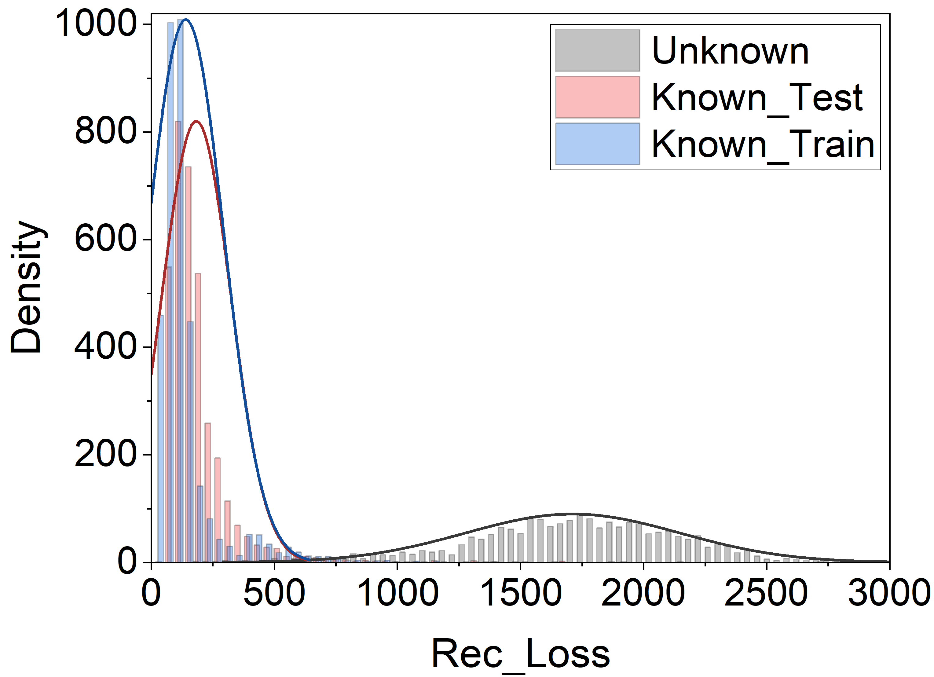
(a) SNR=4dB

(b) SNR=0dB

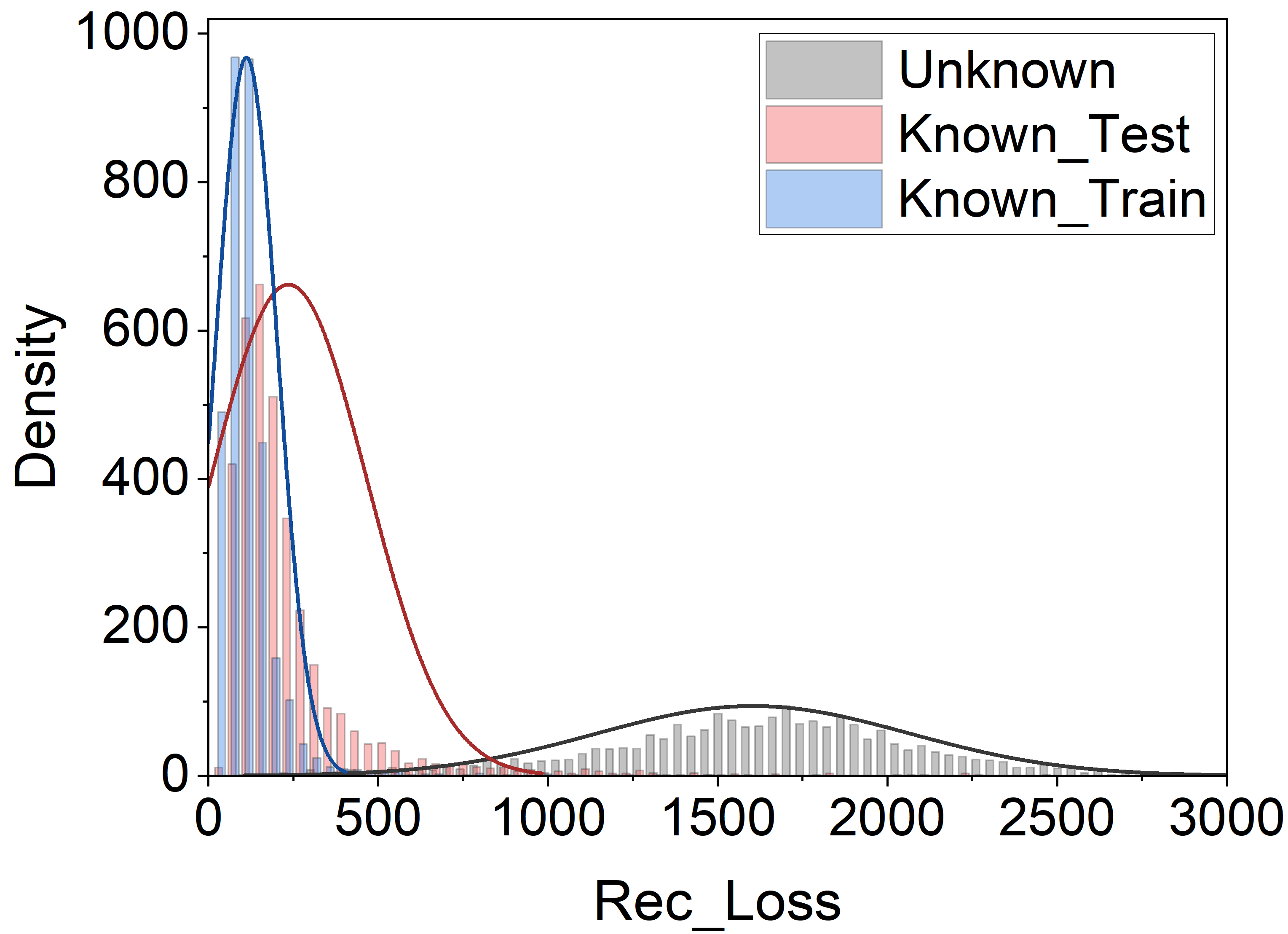
(c) SNR=-4dB

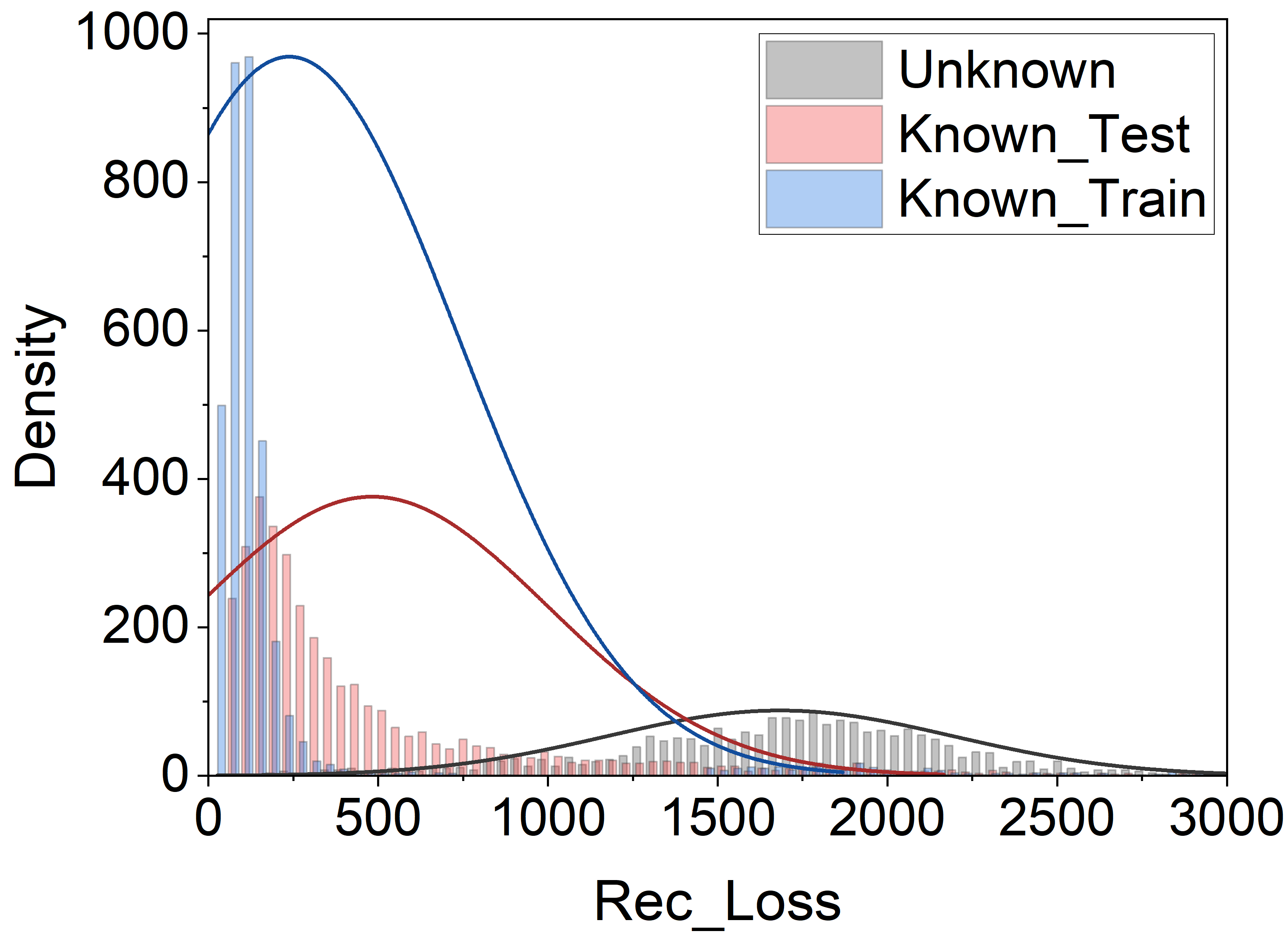
(d) SNR=-8dB

Figure 4: The distribution of reconstruction losses for known and unknown classes at different SNRs.

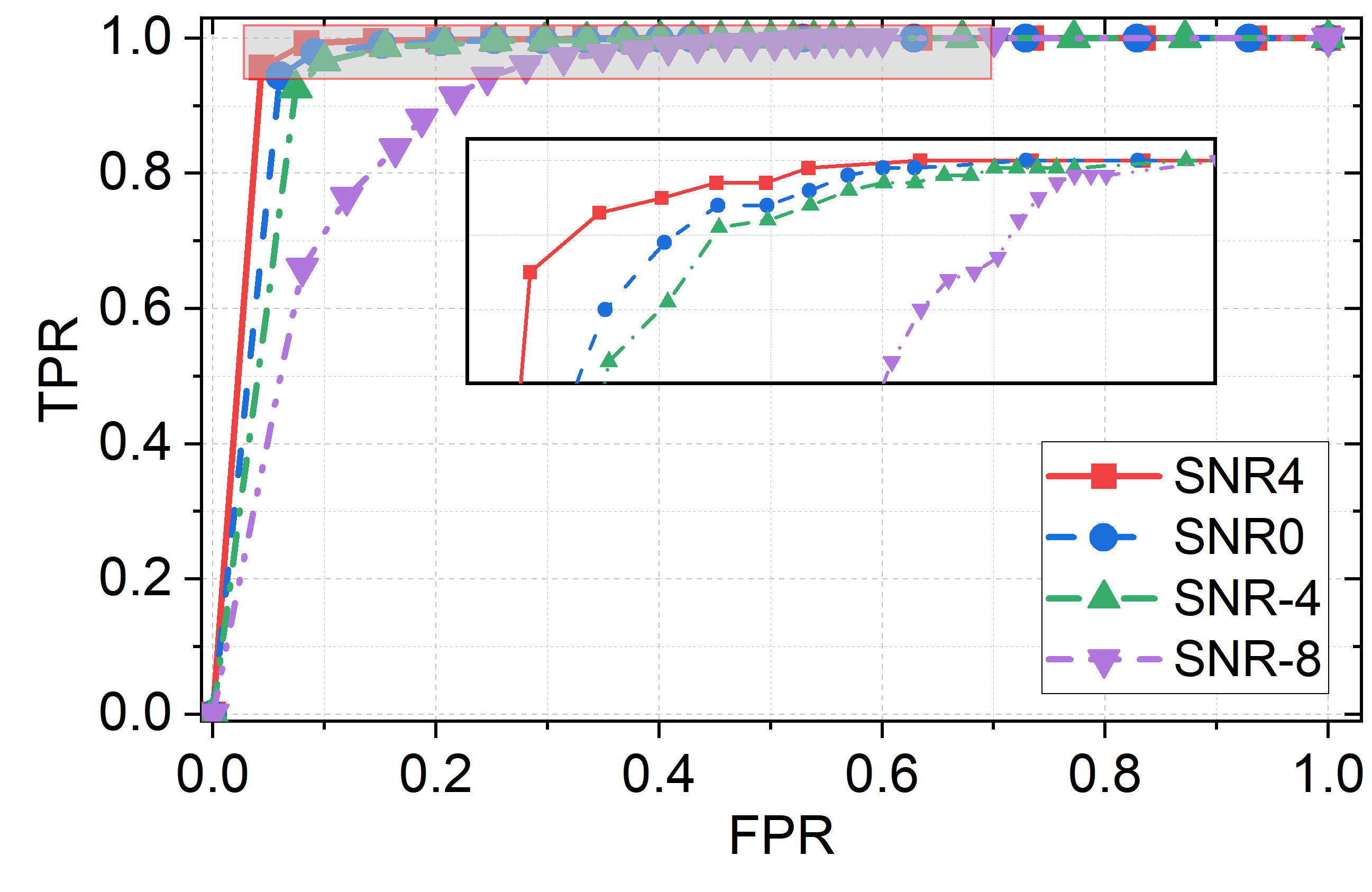
Figure 5: ROC curves at different SNRs.

When the SNR is at $-$4dB or higher, it is visually evident that the distribution of reconstruction losses for the testing known samples is very close to that of the training samples. Additionally, there is minimal overlap between the reconstruction losses of the known samples and the unknown samples. This observation demonstrates the discriminative power of the proposed CIR in effectively separating known and unknown classes. However, there can be some overlap in the reconstruction losses between the known samples and the unknown samples at -8dB due to the influence of noise and increased feature ambiguity.

By changing the threshold, the ROC curves at different SNRs is shown in Fig. 5. As the threshold decreases, the FPR increases while the TPR also increases. A larger area under the ROC curve means a higher TPR at the same FPR, indicating better performance. It can be observed that even at -8dB, the proposed method achieves TPR of 0.765 when FPR is 0.120, which underscores the effectiveness and robustness of the proposed CIR.

V-B2 Ablation Study

The proposed method introduces Restormer for denoising, aiming to improve performance at low SNRs. Additionally, CCVs and MI loss function are elaborately designed to enhance the discrepancy in reconstruction losses between known and unknown classes, thereby achieving better UCI performance. Ablation studies are conducted using different configurations to assess the contributions of the aforementioned design elements. The following configurations are examined: 1) Configuration without Restormer (n-Restormer); 2) Configuration without CCVs (n-CVV); 3) Configuration without MI loss function (n-MI).

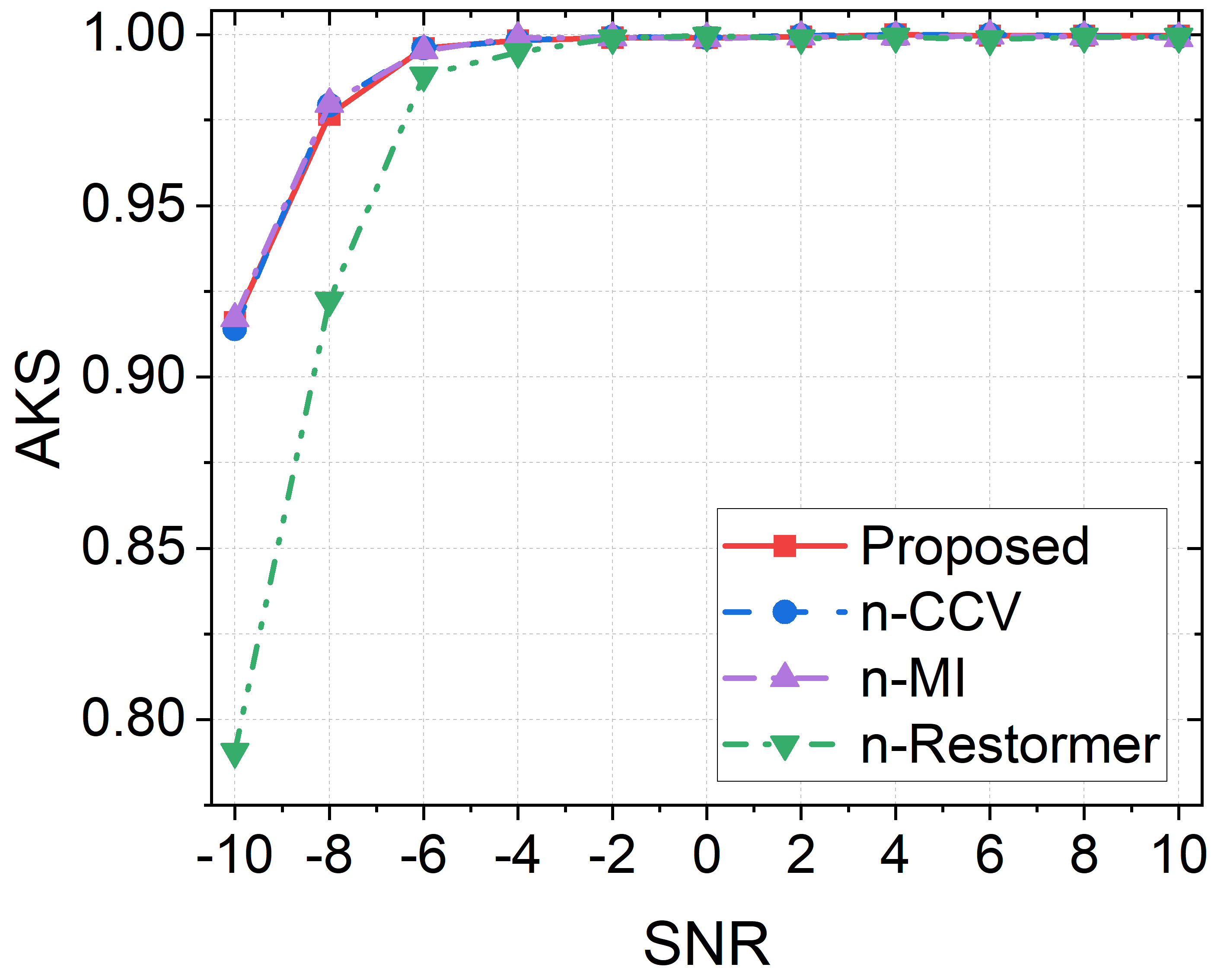
(a) The KCC performance

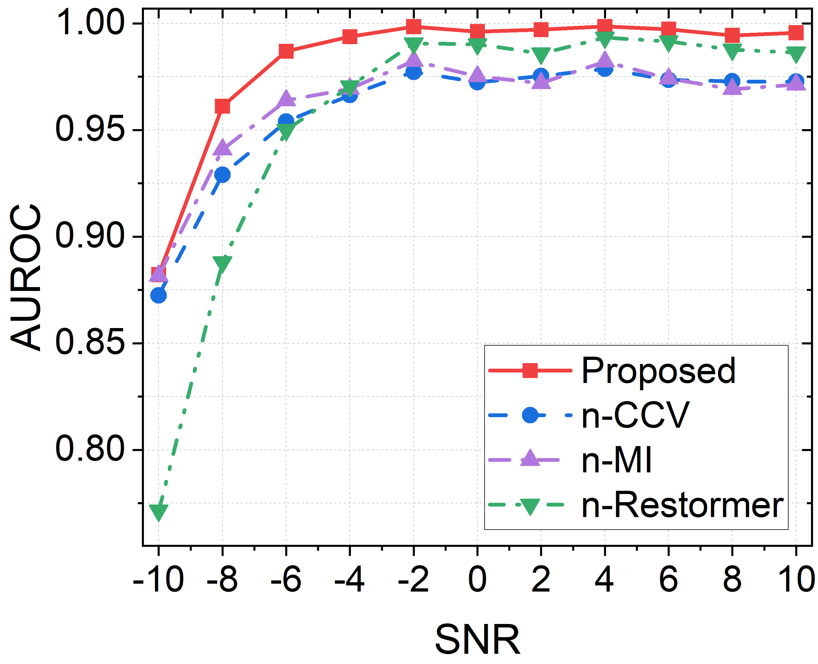
(b) The UCI performance

Figure 6: Performance with different network configurations.

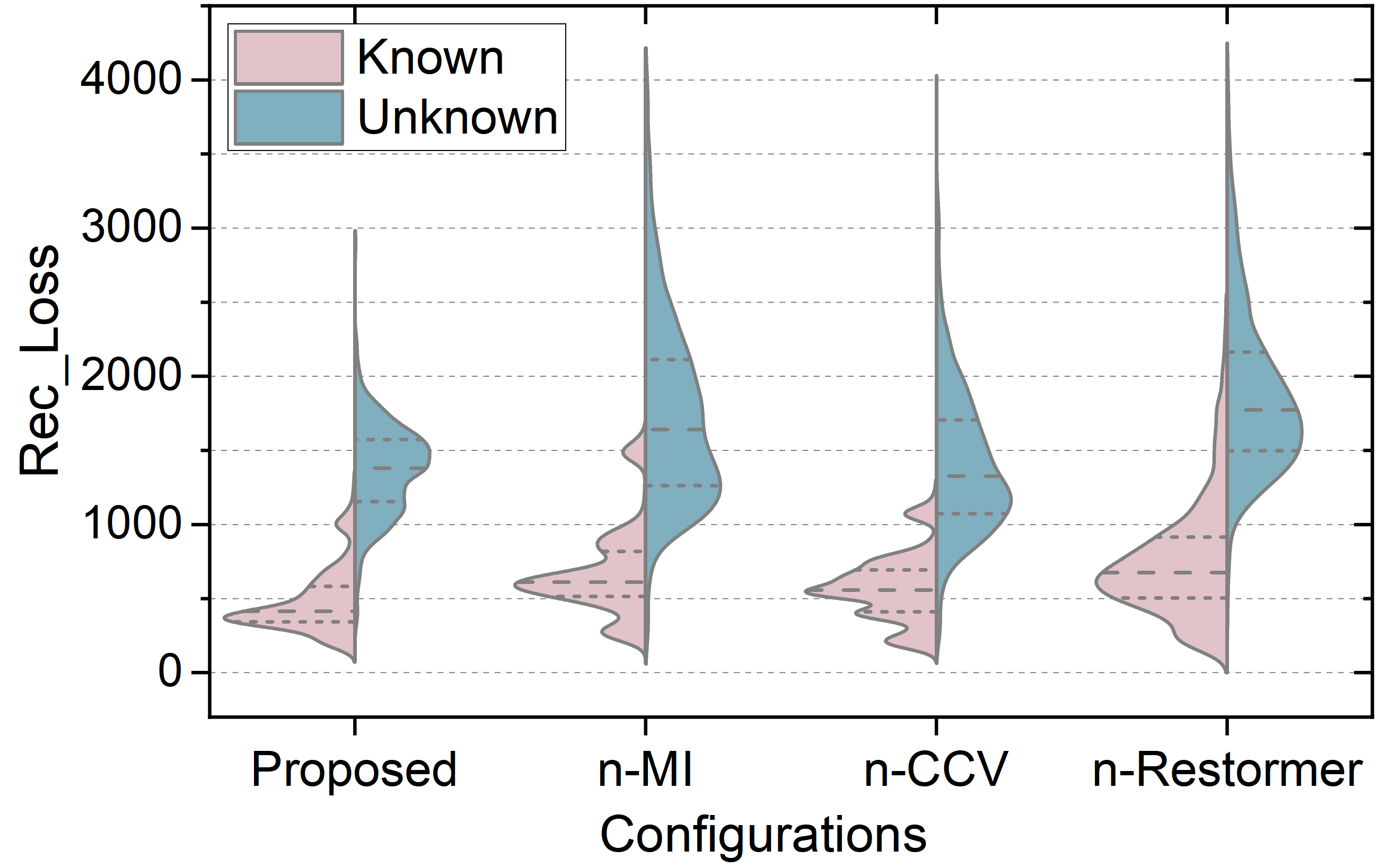
Figure 7: The distribution of reconstruction losses for known and unknown classes at 8dB.

Fig. 6 presents the KCC and UCI performance with different configurations at different SNRs. For the KCC task, when the SNR is above $-$4dB, all configurations achieve an AKS of over 99%. However, as the SNR decreases, it becomes evident that n-Restormer experiences a noticeable decline in performance. At -10dB, the AKS of the n-Restormer is 12.54% lower than the AKS of others. By reducing the noise level, the denoising module improves the quality of the signal, thereby enhancing the KCC performance effectively.

For the UCI task, the proposed CIR consistently exhibits superior performance across a range of SNRs. Interestingly, when the SNR drops below -6dB, the AUROC of n-Restormer is significantly lower than that of n-CCV and n-MI. However, as the SNR increases, the AUROC of n-Restormer surpasses that of n-CCV and n-MI. These results underscore that Restormer contributes enormously to UCI task at low SNRs but the CCVs and MI loss function play the crucial role in improving UCI performance at higher SNRs. To further investigate, we analyze the distributions of reconstruction losses at a relatively high SNR of 8dB in Fig. 7. The results show that the proposed method has significantly smaller peak value and variance for reconstruction losses of known samples compared to other methods. Moreover, the proposed method shows a substantially larger peak value for unknown classes relative to the n-CCV and n-MI, demonstrating that CCVs and MI loss function effectively enlarge the reconstruction discrepancy between known and unknown classes.

V-B3 Performance Against SNR

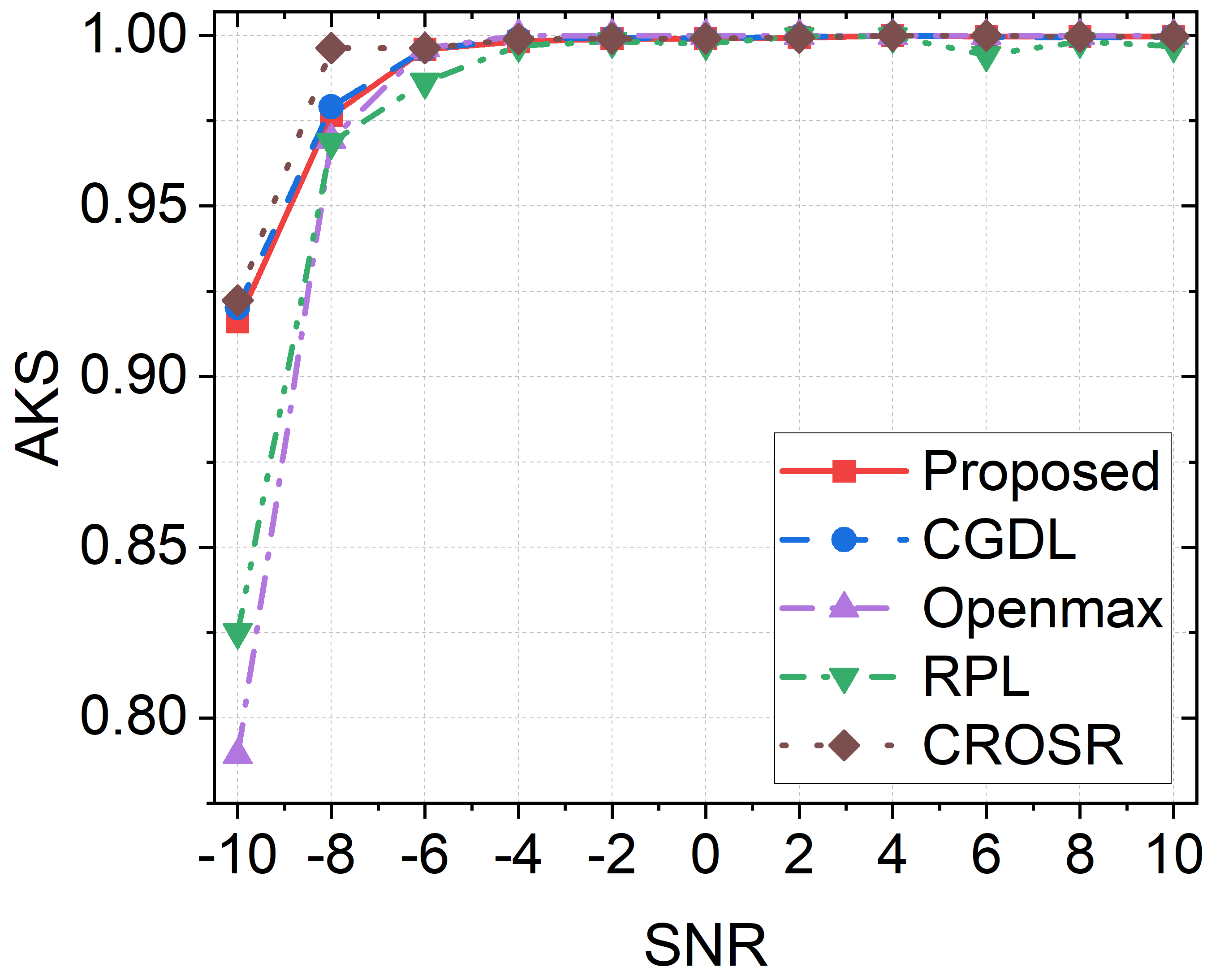
(a) The KCC performance

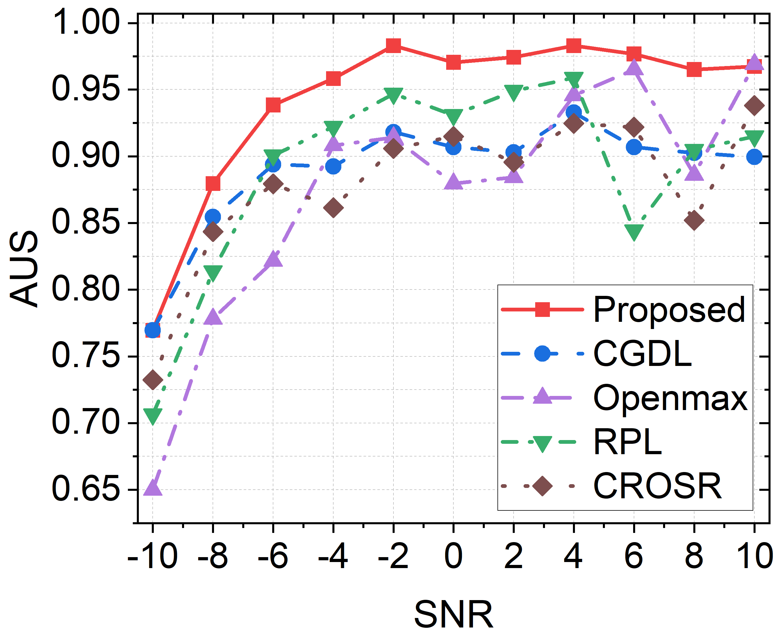
(b) The UCI performance

Figure 8: The performance of different approaches against SNRs.

The Fig. 8 illustrates the performance of the proposed method and baseline methods at different SNRs. For the KCC task, all methods achieve high AKS above 0.99 when the SNR is higher than -4dB. As the SNR decreases, RPL and Openmax exhibit a significant drop in AKS compared to the other methods. It can be observed that the proposed method, CGDL, and CROSR are all AE-based method, showing better KCC performance at low SNRs. This is because the AE compresses the input TFI into a low-dimensional representation and attempts to reconstruct the original input from this representation. This process forces the AE to learn the key features in the data, thereby enhancing the representation capability of the classifier.

For the UCI task, the proposed method demonstrates the best performance across a range of SNRs. It achieves an AUS that is 0.051 higher than the best-performing baseline method at 8dB, and 0.038 higher at -6dB. Moreover, it is worth noting that methods like RPL, Openmax, and CROSR exhibit significant performance fluctuations. For the RPL method, it requires the network to learn the distribution of reciprocal points. Since the distribution of reciprocal points is related to the feature distribution of the data, when the data distribution changes, the distribution of reciprocal points also changes, resulting in unstable network performance. For the Openmax and CROSR methods, the decision thresholds are formulated by calculating the extreme value distribution of features, making them more sensitive to data distribution and leading to unstable UCI performance. In contrast, the proposed method and reconstruction-based methods like CGDL can avoid the issue of unstable UCI performance, since the reconstruction process is not influenced by data distribution.

V-B4 Performance Against Openness

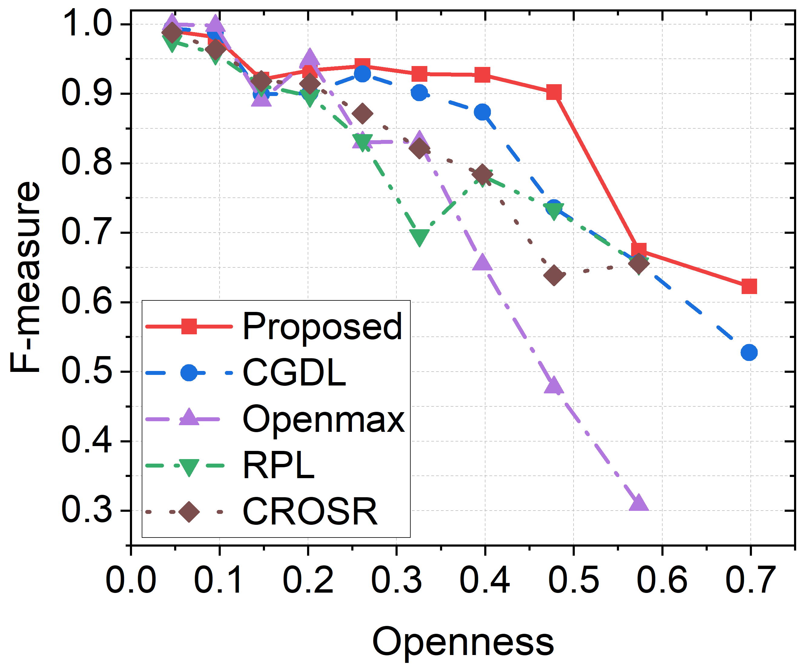
(a) SNR=4dB

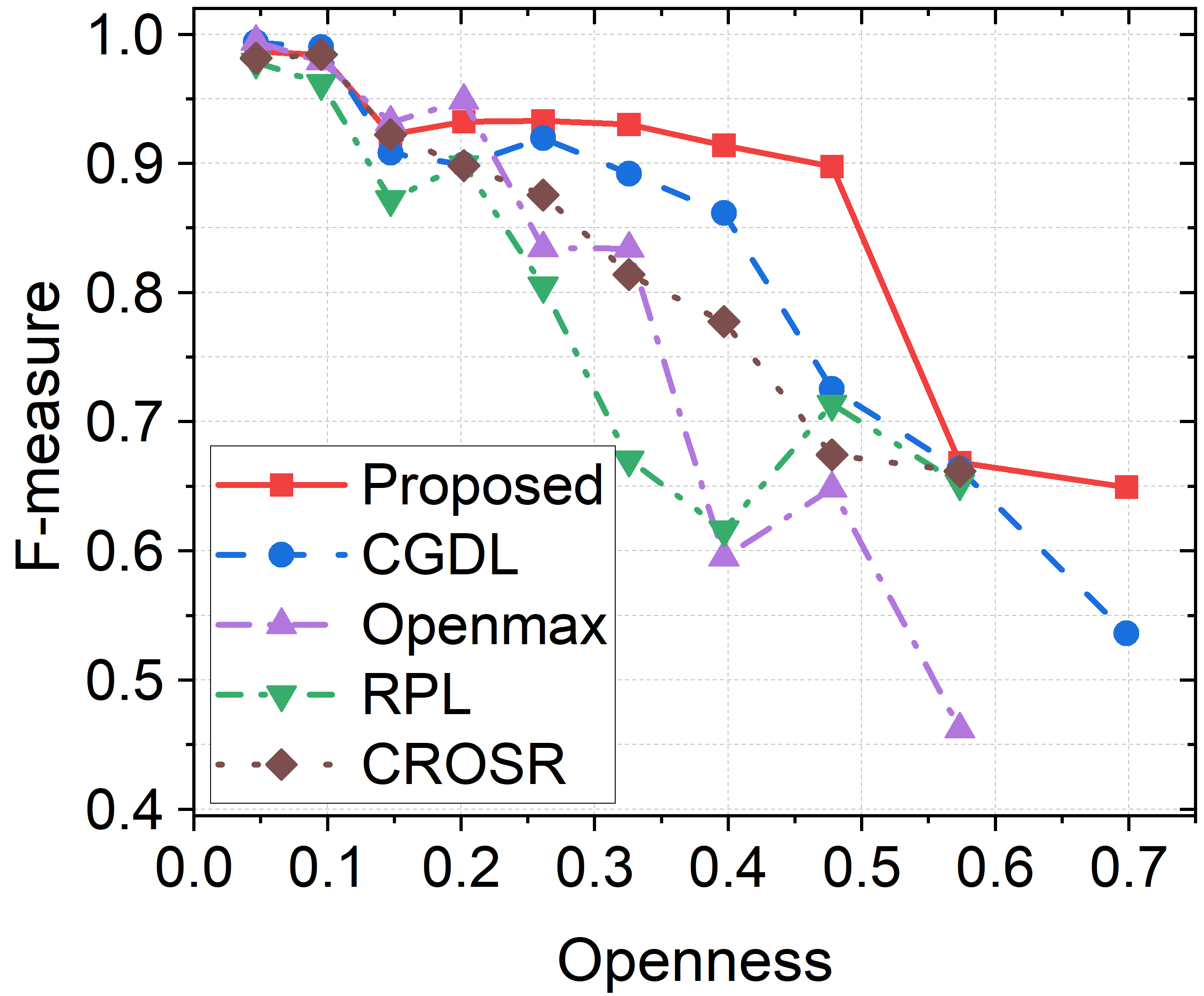
(b) SNR=0dB

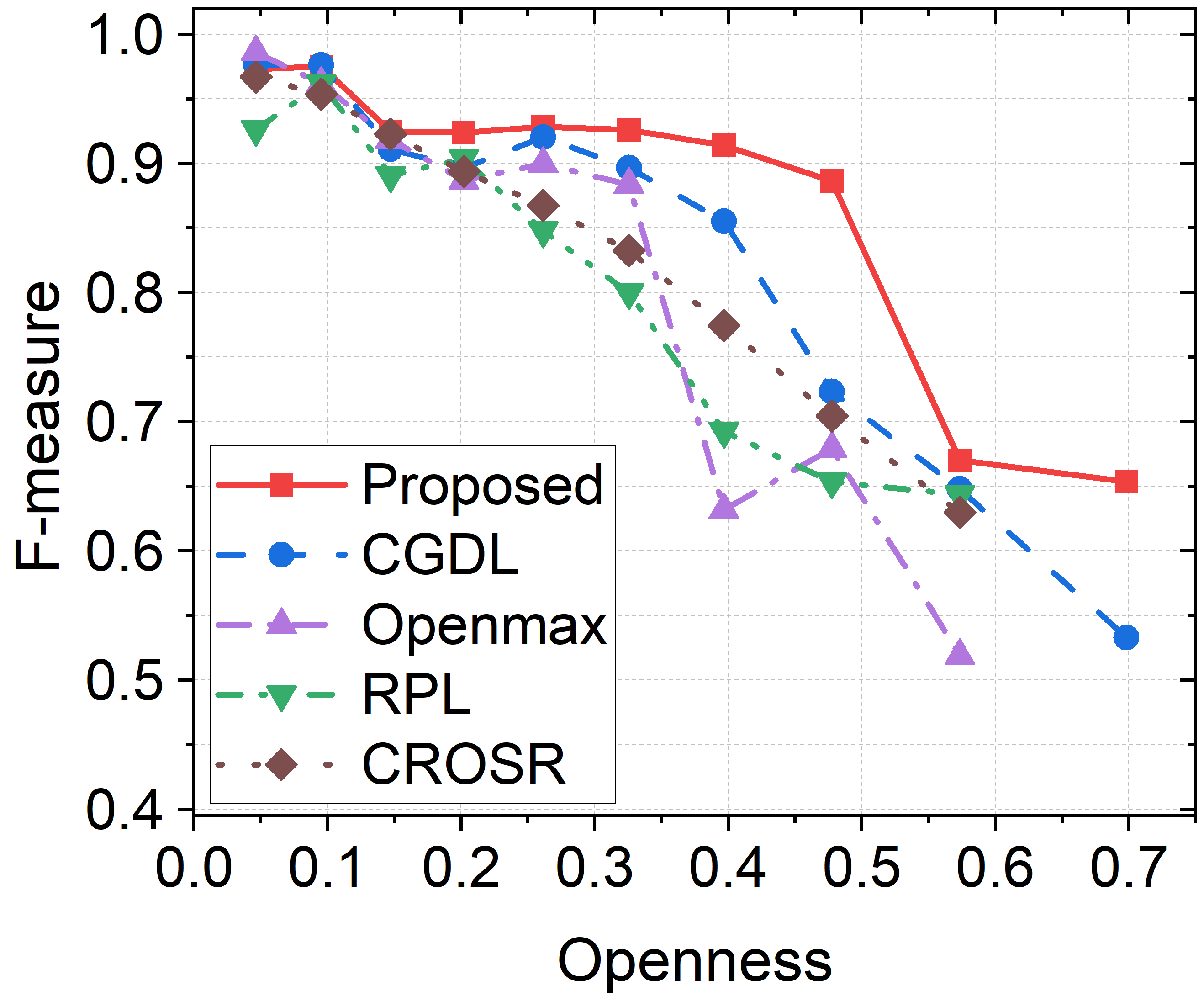
(c) SNR=-4dB

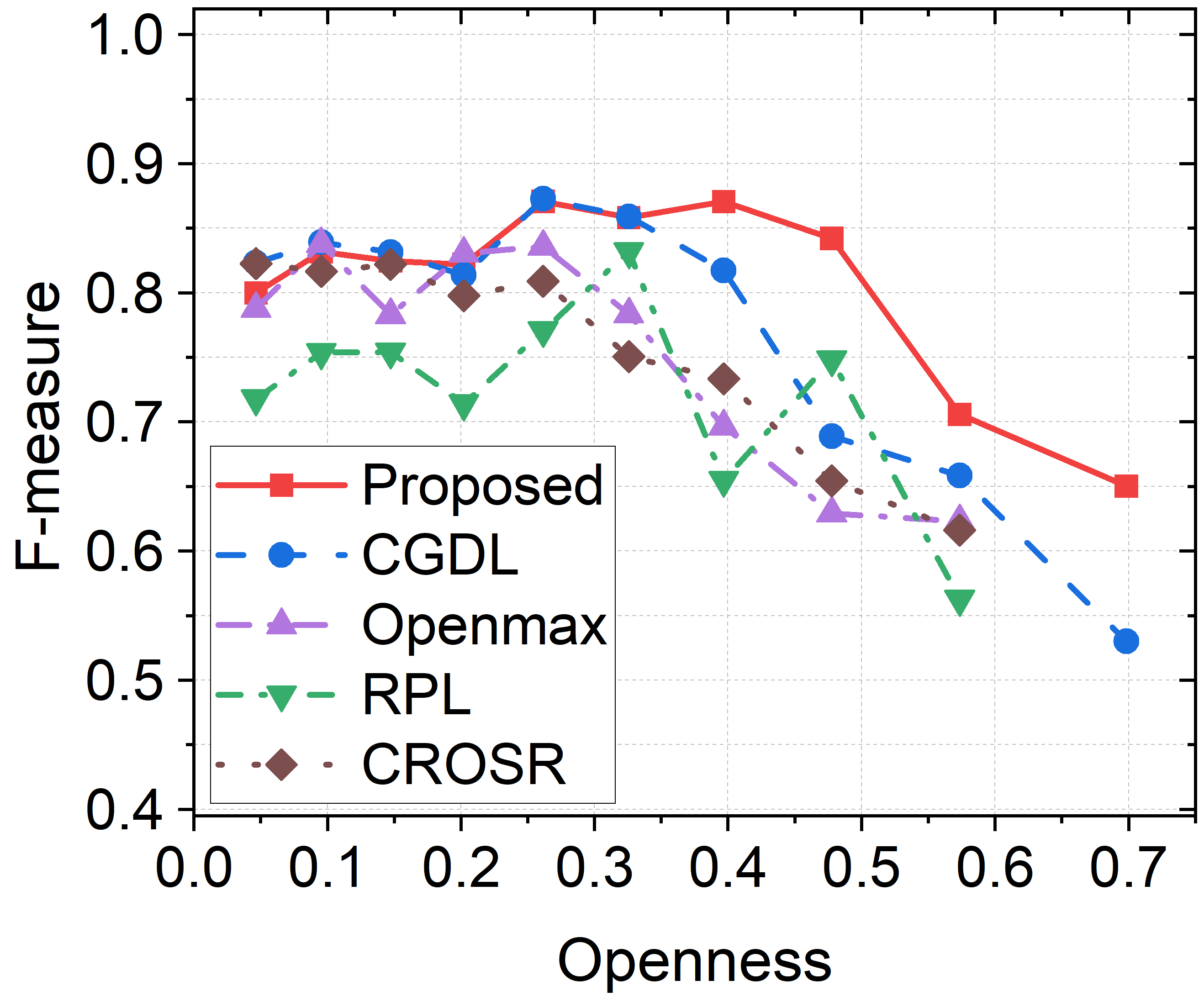
(d) SNR=-8dB

Figure 9: The F-measure performance of different approaches against varying Openness.

The F-measure of the proposed method and the baseline methods against varying openness are presented in Fig. 9. It can be observed that for SNRs of 4dB, 0dB, and -4 dB, all methods achieve an F-measure above 0.85 when the openness is below 0.15. As the openness increases, the F-measure of all methods decreases, whereas the proposed method exhibits superior performance, indicating its capability to handle more complex situations of unknown class discrimination. With an increasing proportion of unknown classes, the data distribution becomes more complex and the boundaries between different classes become blurred, leading to more overlap and intersections between known and unknown samples.

TABLE IV: Performance against different unknown modulation types at -2dB, -6dB and -10dB

SNR	Methods	P1\P2\T1\T3				LFM\Costas\P3\P4				Frank\Costas\T2\T4				P3\P4\T2\T4
		AKS	AUS	NA		AKS	AUS	NA		AKS	AUS	NA		AKS	AUS	NA
-2dB	Proposed	0.9991	0.8985	0.9626		1	0.9604	0.9856		0.9994	0.9647	0.9868		0.9991	0.9720	0.9893
	Openmax	1	0.8922	0.9608		1	0.7284	0.9012		1	0.8255	0.9365		1	0.8978	0.9628
	CGDL	0.9991	0.8389	0.9409		1	0.9247	0.9726		1	0.9535	0.9831		0.9407	0.9871	0.9779
	CROSR	0.9991	0.8793	0.9556		1	0.8764	0.9550		1	0.9196	0.9708		0.9991	0.8640	0.9500
	RPL	0.9980	0.8375	0.9396		0.9986	0.9007	0.9630		0.9963	0.9407	0.9761		0.9977	0.9516	0.9810
-6dB	Proposed	0.9960	0.8836	0.9551		0.9969	0.9305	0.9727		0.9940	0.9364	0.9730		0.9974	0.9455	0.9785
	Openmax	0.9983	0.8769	0.9541		0.9986	0.8195	0.9334		0.9966	0.7829	0.9189		0.9980	0.8509	0.9445
	CGDL	0.9957	0.8338	0.9368		0.9977	0.9069	0.9647		0.9957	0.9295	0.9716		0.9273	0.9819	0.9714
	CROSR	0.9954	0.8665	0.9486		0.9969	0.8796	0.9542		0.9963	0.8753	0.9523		0.9969	0.8511	0.9439
	RPL	0.9791	0.7665	0.9018		0.9874	0.8131	0.9240		0.9906	0.9218	0.9656		0.9763	0.8796	0.9411
-10dB	Proposed	0.9114	0.7178	0.8410		0.9397	0.8102	0.8926		0.9237	0.7724	0.8687		0.9269	0.8109	0.8847
	Openmax	0.8869	0.7287	0.8294		0.8897	0.7029	0.8218		0.8311	0.6662	0.7712		0.8423	0.6993	0.7903
	CGDL	0.9046	0.7302	0.8412		0.9437	0.8229	0.8998		0.9129	0.7655	0.8593		0.8200	0.9154	0.8898
	CROSR	0.9054	0.7091	0.8340		0.2066	0.6244	0.3585		0.9206	0.7287	0.8508		0.9320	0.7247	0.8566
	RPL	0.8726	0.7000	0.8098		0.1931	0.5593	0.3263		0.8660	0.7076	0.8084		0.9034	0.7676	0.8540

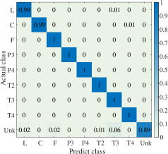
(a) Openness=0.15, SNR=-4dB

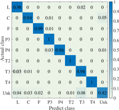
(b) Openness=0.15, SNR=-8dB

(c) Openness=0.57, SNR=-4dB

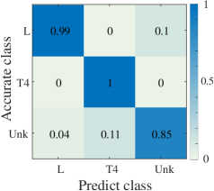
(d) Openness=0.57, SNR=-8dB

Figure 10: The confusion matrices at openness values of 0.15 and 0.57, where the two easily confused modulation type pairs T1&T3 and T2&T4 are introduced.

At openness values of 0.15 and 0.57, there is a noticeable decline in the F-measure. To analyze the underlying causes of the noticeable decline, Fig. 10 provides the confusion matrices at -4dB and -8dB. For openness of 0.15, this can be attributed to the introduction of T1 as a new unknown class. The high similarity between the T1 and T3 modulations means that they can easily be confused and misclassified as each other, leading to the sudden drop of UCI performance. Similarly, at openness 0.57, the introduction of T2 as an unknown class results in significant confusion between T2, T4 and LFM, further impacting the performance negatively.

When the SNR is -8dB, the proposed method shows better performance only when the openness is above 0.33. At openness values of 0.48 and 0.70, the F-measure is 0.1666 and 0.0953 higher than the best baseline method, respectively. Interestingly, the F-measure first increases and then decreases, reaching a peak when the openness is above 0.2 but less than 0.5. This is because F-measure is a metric to evaluate the overall performance. When the openness is low, indicating a lower proportion of unknown categories, the model primarily focuses on the classification task of known categories. Due to the influence of noise and increased feature ambiguity, the model performs poorly in the KCC task, resulting in a decrease in F-measure. When the openness is high, the model performs poorly in the UCI task, leading to a decrease in F-measure.

V-B5 Performance Against Different Unknown Modulation Types

Table IV shows the performance of the proposed method and baseline methods against different unknown modulation types. It can be observed that the proposed method achieves the highest AUCs and NAs when the SNR is at -2dB and -6dB, indicating the best UCI performance. Although the AKSs of Openmax are mostly the highest, they are only higher than the AKSs of proposed method by less than 0.01, so the KCC performance of the two methods can be considered practically equivalent. Therefore, upon comprehensive consideration of the KCC and UCI tasks, it can be argued that the proposed method exhibits the optimal overall performance.

When the SNR is at -10dB, the CGDL method achieves higher AUCs and NAs on the first, second and fourth sub-datasets, while the proposed method generally has higher AKS. It is worth noting that the proposed method performs comparably to CGDL in terms of NAs, with a difference of less than 0.01, so their overall performance can be considered on par. The declining in OSR performance at extremely low SNR (-10dB) could be attributed to overfitting of the more complex networks, resulting in poorer generalization ability of the proposed CIR compared to the simpler CGDL approach. Nevertheless, the proposed method still exhibits better performance in most SNR levels.

Moreover, it is observed that the performance of the proposed method on the first data subset is slightly lower than on the other subsets. A key reason is that the modulation schemes in the first subset (P1, P2, T1, T3) are more complex in nature and thus intrinsically more challenging to recognize compared to those in the other subsets.

V-B6 Performance Validation with Measured Signals

In fact, it is not convincing to evaluate the OSR performance only by testing the methods on the simulated dataset. In this paper, measured signals are obtained by a certain ground-to-air radar to make up a measured signal dataset, which contains signals of five modulation types: Baker7, LFM, NLFM, M15 and Rectangular. Five subsets from the measured signal dataset are constructed to evaluate the AMOSR performance, including three subsets with single unknown class(LFM, NLFM, Baker7) and two subsets with a pair of unknown classes(LFM&NLFM, M15&Baker7). The measured environment is at a horn antenna at a height of 8 meters. The pulse repetition period is 400 $\mu s$, and the pulse width varies between 20 and 60 $\mu s$. The intermediate frequency is 2.2 GHz, and the elevation angle of the receiving antenna is approximately $10^{\circ}$. The sampling frequency is 5 GHz, and the maximum bandwidth of the frequency-modulated waveform is 15 MHz.

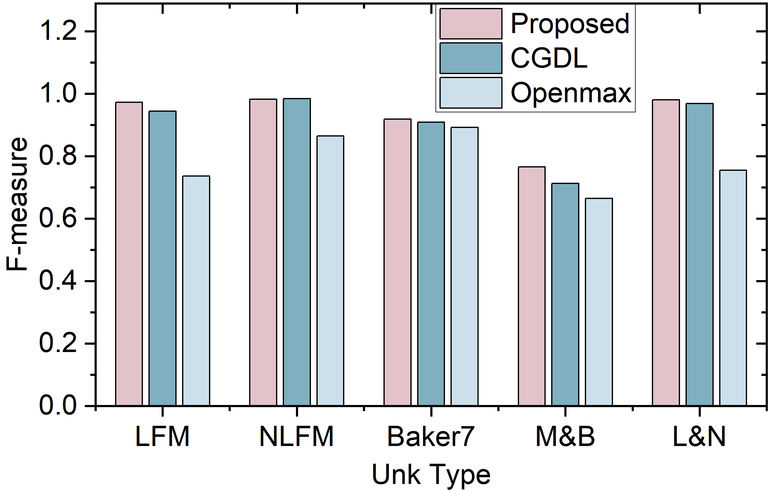
Figure 11: Performance comparison with measured signals.

The F-measure of the proposed method and the two baseline methods with the measured signal dataset are presented in Fig. 11. It can be observed that the reconstruction-based CIR and CGDL approaches significantly outperform the OpenMax and the proposed CIR method achieves better performance than CGDL. Under a difficult scenario where M15 and Baker7 are unknown classes, the F-measure of the proposed CIR is 0.0524 higher than CGDL. The performance is worse when M15 and Baker7 serve as unknown classes because they have relatively more complex modulation patterns compared to other classes. This also explains the evidently lower performance of Baker7 as a single unknown class compared to LFM and NLFM. In summary, the robust performance of the proposed CIR validates the effectiveness of CIR in addressing real-world OSR tasks of high complexity.

VI Conclusion

The paper analyzes two challenging issues in AMOSR: sparse feature distribution and inappropriate decision boundary. To tackle these issues, we propose a class information guided reconstruction framework. The CIR distinguishes known and unknown classes with reconstruction losses, avoiding inappropriate boundary caused by distorted samples. To increase the reconstruction discrepancy between known and unknown classes, we design class conditional vectors and mutual information loss function to refine the latent representations with class information, attaining optimal UCI performance without compromising KCC accuracy, especially in scenarios with a higher proportion of unknown classes. Additionally, a Restormer-based denoising module is introduced before reconstruction, achieving a significant performance improvement over the SNR range of -8dB to 2dB. Experiments on simulated and measured samples validate the effectiveness and robustness of the proposed CIR.

There are several directions that need to be investigated in the future. Firstly, OSR of fingerprint information should be further explored, which is conducive to specific emitter identification and detection of illegal user intrusion. Secondly, most AMOSR methods are performed based on TFIs, whereas the high computational complexity for TFA limits the real-time processing ability of these methods. Therefore, investigating efficient sequence-based OSR methods is necessary for practical applications.

References

- [1] X. Hao, Z. Feng, S. Yang, M. Wang, and L. Jiao, “Automatic modulation classification via meta-learning,” IEEE Internet of Things Journal, vol. 10, no. 14, pp. 12 276–12 292, 2023.
- [2] S. Chang, S. Huang, R. Zhang, Z. Feng, and L. Liu, “Multitask-learning-based deep neural network for automatic modulation classification,” IEEE Internet of Things Journal, vol. 9, no. 3, pp. 2192–2206, 2022.
- [3] L. M. Hoang, M. Kim, and S.-H. Kong, “Automatic recognition of general lpi radar waveform using ssd and supplementary classifier,” IEEE Transactions on Signal Processing, vol. 67, no. 13, pp. 3516–3530, 2019.
- [4] Y. Dong, X. Jiang, H. Zhou, Y. Lin, and Q. Shi, “Sr2cnn: Zero-shot learning for signal recognition,” IEEE Transactions on Signal Processing, vol. 69, pp. 2316–2329, 2021.
- [5] S. Lin, Y. Zeng, and Y. Gong, “Modulation recognition using signal enhancement and multistage attention mechanism,” IEEE Transactions on Wireless Communications, vol. 21, no. 11, pp. 9921–9935, 2022.
- [6] Y. Wang, J. Bai, Z. Xiao, H. Zhou, and L. Jiao, “Msmcnet: A modular few-shot learning framework for signal modulation classification,” IEEE Transactions on Signal Processing, vol. 70, pp. 3789–3801, 2022.
- [7] J. Cai, M. He, X. Cao, and F. Gan, “Semi-supervised radar intra-pulse signal modulation classification with virtual adversarial training,” IEEE Internet of Things Journal, pp. 1–1, 2023.
- [8] B. Dong, Y. Liu, G. Gui, X. Fu, H. Dong, B. Adebisi, H. Gacanin, and H. Sari, “A lightweight decentralized-learning-based automatic modulation classification method for resource-constrained edge devices,” IEEE Internet of Things Journal, vol. 9, no. 24, pp. 24 708–24 720, 2022.
- [9] S. Huang, R. Dai, J. Huang, Y. Yao, Y. Gao, F. Ning, and Z. Feng, “Automatic modulation classification using gated recurrent residual network,” IEEE Internet of Things Journal, vol. 7, no. 8, pp. 7795–7807, 2020.
- [10] B. Ren, K. C. Teh, H. An, and E. Gunawan, “Automatic modulation recognition of dual-component radar signals using resswint–swint network,” IEEE Transactions on Aerospace and Electronic Systems, vol. 59, no. 5, pp. 6405–6418, 2023.
- [11] X. Zhang, H. Zhao, H. Zhu, B. Adebisi, G. Gui, H. Gacanin, and F. Adachi, “Nas-amr: Neural architecture search-based automatic modulation recognition for integrated sensing and communication systems,” IEEE Transactions on Cognitive Communications and Networking, vol. 8, no. 3, pp. 1374–1386, 2022.
- [12] S. Xu, L. Liu, and Z. Zhao, “Dtftcnet: Radar modulation recognition with deep time-frequency transformation,” IEEE Transactions on Cognitive Communications and Networking, vol. 9, no. 5, pp. 1200–1210, 2023.
- [13] K. Chen, L. Wang, J. Zhang, S. Chen, and S. Zhang, “Semantic learning for analysis of overlapping lpi radar signals,” IEEE Transactions on Instrumentation and Measurement, vol. 72, pp. 1–15, 2023.
- [14] Y. Guo, H. Sun, H. Liu, and Z. Deng, “Radar signal recognition based on cnn with a hybrid attention mechanism and skip feature aggregation,” IEEE Transactions on Instrumentation and Measurement, pp. 1–1, 2022.
- [15] Z. Zhang, Y. Li, M. Zhu, and S. Wang, “Jdmr-net: Joint detection and modulation recognition networks for lpi radar signals,” IEEE Transactions on Aerospace and Electronic Systems, pp. 1–15, 2023.
- [16] L. Zhang, S. Lambotharan, G. Zheng, G. Liao, B. AsSadhan, and F. Roli, “Attention-based adversarial robust distillation in radio signal classifications for low-power iot devices,” IEEE Internet of Things Journal, vol. 10, no. 3, pp. 2646–2657, 2023.
- [17] P. Ghasemzadeh, M. Hempel, and H. Sharif, “Gs-qrnn: A high-efficiency automatic modulation classifier for cognitive radio iot,” IEEE Internet of Things Journal, vol. 9, no. 12, pp. 9467–9477, 2022.
- [18] K. Chen, J. Zhang, S. Chen, S. Zhang, and H. Zhao, “Recognition and estimation for frequency-modulated continuous-wave radars in unknown and complex spectrum environments,” IEEE Transactions on Aerospace and Electronic Systems, vol. 59, no. 5, pp. 6098–6111, 2023.
- [19] J. Yang, K. Zhou, Y. Li, and Z. Liu, “Generalized out-of-distribution detection: A survey,” arXiv preprint arXiv:2110.11334, 2021.
- [20] W. J. Scheirer, A. de Rezende Rocha, A. Sapkota, and T. E. Boult, “Toward open set recognition,” IEEE Transactions on Pattern Analysis and Machine Intelligence, vol. 35, no. 7, pp. 1757–1772, 2013.
- [21] M. Salehi, H. Mirzaei, D. Hendrycks, Y. Li, M. Rohban, M. Sabokrou et al., “A unified survey on anomaly, novelty, open-set, and out of-distribution detection: Solutions and future challenges,” Transactions on Machine Learning Research, no. 234, 2022.
- [22] T. Li, Z. Wen, Y. Long, Z. Hong, S. Zheng, L. Yu, B. Chen, X. Yang, and L. Shao, “The importance of expert knowledge for automatic modulation open set recognition,” IEEE Transactions on Pattern Analysis and Machine Intelligence, vol. 45, no. 11, pp. 13 730–13 748, 2023.
- [23] P. Schlachter, Y. Liao, and B. Yang, “Open-set recognition using intra-class splitting,” in 2019 27th European signal processing conference (EUSIPCO). IEEE, 2019, pp. 1–5.
- [24] Y. Xu, X. Qin, X. Xu, and J. Chen, “Open-set interference signal recognition using boundary samples: A hybrid approach,” in 2020 International Conference on Wireless Communications and Signal Processing (WCSP). IEEE, 2020, pp. 269–274.
- [25] H. Xu and X. Xu, “A transformer based approach for open set specific emitter identification,” in 2021 7th International Conference on Computer and Communications (ICCC). IEEE, 2021, pp. 1420–1425.
- [26] G. Chen, L. Qiao, Y. Shi, P. Peng, J. Li, T. Huang, S. Pu, and Y. Tian, “Learning open set network with discriminative reciprocal points,” in Computer Vision–ECCV 2020: 16th European Conference, Glasgow, UK, August 23–28, 2020, Proceedings, Part III 16. Springer, 2020, pp. 507–522.
- [27] H.-M. Yang, X.-Y. Zhang, F. Yin, Q. Yang, and C.-L. Liu, “Convolutional prototype network for open set recognition,” IEEE Transactions on Pattern Analysis and Machine Intelligence, vol. 44, no. 5, pp. 2358–2370, 2020.
- [28] G. Chen, P. Peng, X. Wang, and Y. Tian, “Adversarial reciprocal points learning for open set recognition,” IEEE Transactions on Pattern Analysis and Machine Intelligence, vol. 44, no. 11, pp. 8065–8081, 2021.
- [29] D. Hendrycks and K. Gimpel, “A baseline for detecting misclassified and out-of-distribution examples in neural networks,” in International Conference on Learning Representations, 2016.
- [30] A. Bendale and T. E. Boult, “Towards open set deep networks,” in Proceedings of the IEEE conference on computer vision and pattern recognition, 2016, pp. 1563–1572.
- [31] H. Huang, Y. Wang, Q. Hu, and M.-M. Cheng, “Class-specific semantic reconstruction for open set recognition,” IEEE transactions on pattern analysis and machine intelligence, vol. 45, no. 4, pp. 4214–4228, 2022.
- [32] X. Sun, Z. Yang, C. Zhang, K.-V. Ling, and G. Peng, “Conditional gaussian distribution learning for open set recognition,” in Proceedings of the IEEE/CVF Conference on Computer Vision and Pattern Recognition, 2020, pp. 13 480–13 489.
- [33] R. Yoshihashi, W. Shao, R. Kawakami, S. You, M. Iida, and T. Naemura, “Classification-reconstruction learning for open-set recognition,” in Proceedings of the IEEE/CVF Conference on Computer Vision and Pattern Recognition, 2019, pp. 4016–4025.
- [34] L. Buquicchio, W. Gerych, A. Alajaji, K. Chandrasekaran, H. Mansoor, T. Hartvigsen, E. Rundensteiner, and E. Agu, “Variational open set recognition (vosr),” in 2021 IEEE International Conference on Big Data (Big Data). IEEE, 2021, pp. 994–1001.
- [35] J. Sun, H. Wang, and Q. Dong, “Moep-ae: Autoencoding mixtures of exponential power distributions for open-set recognition,” IEEE Transactions on Circuits and Systems for Video Technology, vol. 33, no. 1, pp. 312–325, 2022.
- [36] X. Zhang, X. Cheng, D. Zhang, P. Bonnington, and Z. Ge, “Learning network architecture for open-set recognition,” in Proceedings of the AAAI Conference on Artificial Intelligence, vol. 36, no. 3, 2022, pp. 3362–3370.
- [37] R. V. Chakravarthy, H. Liu, and A. M. Pavy, “Open-set radar waveform classification: Comparison of different features and classifiers,” in 2020 IEEE International Radar Conference (RADAR). IEEE, 2020, pp. 542–547.
- [38] C. T. Fredieu, A. Martone, and R. M. Buehrer, “Open-set classification of common waveforms using a deep feed-forward network and binary isolation forest models,” in 2022 IEEE Wireless Communications and Networking Conference (WCNC). IEEE, 2022, pp. 2465–2469.
- [39] X. Han and S. Chen, “Open-set recognition of lpi radar signals based on deep class probability output network,” in 2022 IEEE 8th International Conference on Computer and Communications (ICCC). IEEE, 2022, pp. 193–198.
- [40] Y. Chen, X. Xu, and X. Qin, “An open-set modulation recognition scheme with deep representation learning,” IEEE Communications Letters, vol. 27, no. 3, pp. 851–855, 2023.
- [41] W. Yu, A. Lin, Z. Ma, Z. Huang, and Y. Xia, “Unknown radar signal recognition technology based on ds evidence theory,” in 2021 IEEE 2nd International Conference on Big Data, Artificial Intelligence and Internet of Things Engineering (ICBAIE). IEEE, 2021, pp. 440–445.
- [42] W. Zhang, D. Huang, M. Zhou, J. Lin, and X. Wang, “Open-set signal recognition based on transformer and wasserstein distance,” Applied Sciences, vol. 13, no. 4, p. 2151, 2023.
- [43] J. Gong, X. Qin, and X. Xu, “Multi-task based deep learning approach for open-set wireless signal identification in ism band,” IEEE Transactions on Cognitive Communications and Networking, vol. 8, no. 1, pp. 121–135, 2021.
- [44] A. Lin, Z. Ma, Z. Huang, Y. Xia, and W. Yu, “Unknown radar waveform recognition based on transferred deep learning,” IEEE Access, vol. 8, pp. 184 793–184 807, 2020.
- [45] X. Zhang, T. Li, P. Gong, R. Liu, X. Zha, and W. Tang, “Open set recognition of communication signal modulation based on deep learning,” IEEE Communications Letters, vol. 26, no. 7, pp. 1588–1592, 2022.
- [46] S.-H. Kong, M. Kim, L. M. Hoang, and E. Kim, “Automatic lpi radar waveform recognition using cnn,” Ieee Access, vol. 6, pp. 4207–4219, 2018.
- [47] S. W. Zamir, A. Arora, S. Khan, M. Hayat, F. S. Khan, and M.-H. Yang, “Restormer: Efficient transformer for high-resolution image restoration,” in Proceedings of the IEEE/CVF conference on computer vision and pattern recognition, 2022, pp. 5728–5739.
- [48] W. Shi, J. Caballero, F. Huszár, J. Totz, A. P. Aitken, R. Bishop, D. Rueckert, and Z. Wang, “Real-time single image and video super-resolution using an efficient sub-pixel convolutional neural network,” in Proceedings of the IEEE conference on computer vision and pattern recognition, 2016, pp. 1874–1883.
- [49] O. Ronneberger, P. Fischer, and T. Brox, “U-net: Convolutional networks for biomedical image segmentation,” in Medical Image Computing and Computer-Assisted Intervention–MICCAI 2015: 18th International Conference, Munich, Germany, October 5-9, 2015, Proceedings, Part III 18. Springer, 2015, pp. 234–241.
- [50] A. A. Alemi, I. Fischer, J. V. Dillon, and K. Murphy, “Deep variational information bottleneck,” arXiv preprint arXiv:1612.00410, 2016.