A novel boundary-integral algorithm for nonlinear unsteady surface and interfacial waves
Abstract
We devise a new time-stepping algorithm for two-dimensional nonlinear unsteady surface and interfacial waves. The algorithm uses Cauchy’s integral formula, which only requires information on the interface, to solve Laplace equation by using iterative techniques. We derive Eulerian and mixed Eulerian-Lagrangian descriptions by using arclength to parameterize the interface which is updated through its inclination angle and velocity potential at each time step. The algorithm shows broad applicability and excellent numerical accuracy in various numerical simulations, including wave breaking, collisions of solitary waves, vortex roll-up, etc. We especially focus on the stability of symmetric interfacial gravity-capillary solitary waves in deep water. Linear stability analysis is performed using a new formulation which possesses excellent numerical efficiency and robustness. It is shown that the depression/elevation solitary waves are linearly stable/unstable except the portion where the monotonicity of energy curve changes firstly. These results are supported by our fully nonlinear simulations, especially the head-on collisions of solitary waves.
1 Introduction
Waves on the interfaces of two immersible fluids are known as interfacial waves. As an extension of water waves, they can date back to Kelvin and Helmholtz in their studies of hydrodynamic instabilities. Many physical related scenarios can be effectively modelled by interfacial waves, for instance, air-water interactions, oceanic internal waves, etc. These phenomena are usually highly nonlinear and can not be well described by weakly nonlinear models, such as the Korteweg–de Vries equation or the nonlinear Schrödinger (NLS) equation, leaving nonlinear simulations to be the only approach in many cases.
As a special case of interfacial waves, water waves have been numerically simulated for decades and proven to be an active and fruitful area. Under the three classical assumptions, i.e. the flow is incompressible, irrotational, and inviscid, the Euler equations are equivalent to the Laplace equation with boundary conditions on a time-dependent surface. This enables to use numerical methods of boundary-integral type, which have advantages of reducing the dimensionality of the original problems. In two dimensions, these numerical algorithms can be approximately separated into three kinds: (1) Green’s function method based on Green’s identities [17, 30], (2) Cauchy’s integral method based on Cauchy’s integral formula for analytic functions [10, 20], and (3) vortex method based on singularity distributions and the Biot-Savart integral [1]. Sample points are initially spread on the surface and labelled by a parameter . Their physical coordinates are tracked during the simulation. This is the essence of the Lagrangian description, which is popular due to its simple mathematical formulation. The particle-tracking strategy offers adaptability, allowing sample particles to cluster in regions of high curvature, which is especially attractive when studying breaking waves [17]. On the other hand, the Eulerian description fixes the positions of sample points in the physical space, e.g. their -coordinates, or in some transformation spaces [20, 23], usually leading to complicated formulations.
When it comes to two-fluid system, adopting the same assumptions as in the water waves gives benefits to simplifying the mathematical formulation of interfacial waves, especially by allowing the application of boundary-integral methods. The inviscid assumption leads to a discontinuity in tangential velocity across the interface. Since flows are irrotational in the interior of fluid, vorticity is confined to the interface, making it a vortex sheet with zero thickness. Therefore, the vortex method is especially popular in studies of interfacial motions [2, 22, 13, 14], including wave propagation, instabilities of the Rayleigh-Taylor (R-T) and Kelvin-Helmholtz (K-H) type, etc. Boundary-integral methods based on Cauchy’s integral formula, although less commonly used, have advantages in situations where topography plays a crucial role. To our knowledge, the only application in unsteady interfacial waves via this approach is [11] where the authors investigated unsteady transcritical two-layer flow over a bottom topography. Their method is a direct extension of that in [10] for surface waves, based on the Lagrangian description.
In many situations, surface tension is important for interfacial waves, either physically relevant or as a regularization of the K-H singularity. In this context, Eulerian description or mixed Eulerian-Lagrangian description are better choices because Lagrangian description may lead to an overly sparse distribution of sample particles, resulting in poor physical resolution. In [2], the authors found that sample particles tend to move away from the developing spike and bubble regions, thus restricting the numerical accuracy. In addition, the accumulation of particles increases local wave number and may cause severe numerical stiffness, as reported in [13]. A natural parameterization for Eulerian description is to use the arclength , which guarantees a uniform distribution of sample points on the interface regardless of the topology of waves. The physical coordinates of these points, as well as their velocity potential values are the unknowns to be solved, leading to a discretized system with unknowns, where is the number of sample points on the interface. Alternatively, a more convenient approach is to use the inclination angle of the interface as unknown. This only requires unknowns and leads to a formulation.
In this paper, we describe a new boundary-integral algorithm to simulate two-dimensional nonlinear interfacial waves and surface waves. The basic idea is to use a pair of functions: and , to describe the motion of interface or surface, where is a density-weighted velocity potential defined in section 3.1.4. To integrate these unknowns in time, normal velocity on the interface is required. Given and , is determined from Cauchy’s integral formula, which is reformulated into a Fredholm integral equation of the second kind. This equation is solved iteratively by using the generalized minimal residual method (GMRES). Note that this idea is analogue to the Hamiltonian formulation of water waves and interfacial waves that uses (surface elevation) and as a pair of canonical variables and Dirichlet-to-Neumann operator to solve [31, 4]. To derive an Eulerian description, we adopt an arclength-parameterization method to ensure uniform spacing of sample points along the interface or surface. It is worth noting that two other works have employed a very similar concept. In [30], the author used a combination of formulation and Green’s function to study a fluid falling into vacuum. In [13], formulation coupled with vortex sheet method is employed to study Hele-Shaw flow and vortex roll-up structures due to the K-H instability.
Using the combination of formulation and Cauchy’s integral formula, we are able to simulate various wave phenomena, such as wave breaking, collision of solitary waves, vortex roll-up, etc. Particularly, we focus on the stability of symmetric interfacial gravity-capillary solitary waves in deep water. To our knowledge, there are few works on this topic due to the lack of good algorithms for unsteady interfacial waves. In [5], the authors studied the linear stability of surface gravity-capillary solitary waves in deep water. There are two kinds of symmetric solitary waves which feature negative and positive values of on their center in small amplitude, known as depression and elevation solitary waves (see Fig. 5 and 6). It was found that the depression solutions are linearly stable. On the other hand, the elevation solutions are linearly unstable until a stationary point of energy emerges on their bifurcation. Subsequently, solutions become linearly stable until a second stationary appears. These findings are supported by the theory of exchange of stability [24] in superharmonic case and various nonlinear numerical experiments [18, 28]. In [6], the authors extended the linear stability analysis to interfacial gravity-capillary solitary waves in a shallow water-deep water setting and found that the linear stability is density-dependent. To our knowledge, this is the only work regarding the linear stability of interfacial gravity-capillary solitary waves. We have used the same method derived in [6] but encountered some numerical issues. The problem is intrinsic to their formulation which has a form of generalised eigenvalue problems: , where and are matrices, and especially is singular. To address this, we reformulate the analysis, partly inspired by the formulation, by introducing new variables. This ultimately gives rise to a eigenvalue problem in standard form, possessing both numerical robustness and efficiency. This formulation are employed to interfacial gravity-capillary solitary waves in deep water, for a fixed density ratio . It is found that for depression solitary waves, their energy bifurcation has two stationary points and the solutions between them are linearly unstable. For elevation solitary waves, their linear stability properties are almost same to that were previously found for surface elevation solitary waves, except there is a dominant superharmonic instability before the second exchange of stability happens. These results are supported by our fully nonlinear simulations that use perturbed solitary waves as the initial conditions and monitor the growth of the disturbances. We also perform head-on collisions between solitary waves, which yield the same conclusions on their stability. It is worth mentioning that we found our time-stepping algorithm is numerically robust and very accurate in long-term simulations.
2 Mathematical formulation
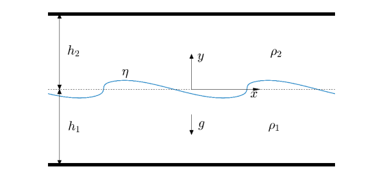
We consider a system composed of two immersible, incompressible and inviscid fluids with different densities (see Fig. 1). The lighter fluid lies above the heavier one to keep a linearly stable configuration. Inside each fluid, we assume that the motion is two-dimensional and irrotational. Thus we can introduce two velocity potential functions , where subscripts are used to represent properties of the the lower and upper fluid. We also assume that each fluid has uniform depth and constant density . Thus we can write down the Laplace equation in each fluid layer
| (1) | ||||
| (2) |
where we have used to denote the elevation of the interface and put the -axis on the mean water level. On the interface, two kinematic boundary conditions and a dynamic boundary condition are imposed
| (3) | ||||
| (4) | ||||
| (5) |
where is the acceleration due to the gravity, and is the coefficient of surface tension. On the top and bottom wall, we impose two impermeability boundary conditions
| (6) | ||||
| (7) |
By choosing
| (8) |
as typical length, speed and time scales, we make the above formulation dimensionless. Eqs. (1)-(4), (6), and (7) are invariant. The dynamic boundary condition (5) now reads
| (9) |
where represents the density ratio.
Linearizing the system and assuming solutions are of the following forms,
| (10) | ||||
| (11) | ||||
| (12) |
where denotes complex conjugate, and to are unknown constants. Solving these coefficients, we can get the dispersion relation
| (13) |
where and represent angular frequency and wave number of linear waves respectively. Since , the right hand side of (13) is always non-negative, thus we have a linearly stable system. If we let , we get the dispersion relation for deep-water waves
| (14) |
3 formulation
3.1 Interfacial waves
Our aim is to derive a formulation for unsteady interfacial waves using the Eulerian or mixed Eulerian-Lagrangian description. It is natural to use arclength , instead of the -coordinate, to parameterize the interface since it could develop overhanging profiles. Without loss of generality, we assume the range of is , where is the total arclength. For the convenience of discretization, we introduce the pseudo-arclength whose range is always . The motion of a Lagrangian particle on the interface is determined by its Cartesian coordinates and , which satisfy the following constraint
| (15) |
Therefore, a more convenient way is to introduce the inclination angle such that
| (16) |
Eq. (15) is then automatically satisfied and we can construct the interface from and by integrating (16). This formulation has benefit by reducing the number of unknowns from to , where is the number of sample points on the interface.
3.1.1 Equation for
Taking an infinitesimal interface element with length , the material derivative of is
| (17) |
where denotes the tangential velocity of the interface, and is the normal velocity (see Appendix A). Note that , but from the kinematic boundary conditions. Therefore, we shall drop the subscript of and use hereafter. For periodic waves, we integrate Eq. (17) and obtain the time-derivative of
| (18) |
where we have used the periodicity of .
3.1.2 Function
From (17), we can also obtain the material derivative of
| (19) |
where can be an arbitrary function. Note that and are independent variables, so . On the other hand, because for the same Lagrangian particle, its value changes with time. We can choose specific forms for and they have different physical meanings. A natural choice is to set , which is equivalent to say at . The physical meaning is that we always fix onto the leftmost fluid particle. Without loss of generality, we let in (19) hereafter. Another computationally convenient choice is to set onto the left boundary of the computational domain. One can then show that (see Appendix B). Hereafter, we shall denote the two choices by Case I and Case II
| (20) |
Note that Case I belongs to the mixed Eulerian-Lagrangian description and Case II is an Eulerian description.
3.1.3 Equation for
3.1.4 Equation for
In the Bernoulli equation (9), the velocity potentials and are coupled together. Therefore, we introduce a density-weighted potential function
| (25) |
Note that denotes the value of evaluated on the interface. Taking the -derivative, we get the density-weighted tangential velocity
| (26) |
The material derivative of is
| (27) |
On the other hand, we have
| (28) |
Combining these and the Bernoulli equation, we can get the equations for and
| (29) | ||||
| (30) |
Using the Young-Laplace condition
| (31) |
to eliminate pressure , we obtain the equation for
| (32) |
3.1.5 Equations for and
The interface can be constructed by integrating (16)
| (33) | ||||
| (34) |
Depending on the choice of function , the equations for and are
| (35) |
| (36) |
It should be pointed out that the Case II choice is not always safe due to the possibility of when waves become overhanging. Therefore, we prefer using Case I when there exist a potential of overturned waves. In the simulations, we expect that volume conservation is satisfied for all time
| (37) |
This provides another way to determine without involving (36) in computations.
3.1.6 Equation for
The mapping from to is the so called Dirichlet-to-Neumann operator in the theory of water waves. In our algorithm, we establish this relationship from boundary integral equations. For periodic waves with wave number , we introduce the following complex mapping
| (38) |
which maps the physical region in a single spatial period to an annular region on the -plane. Since the complex velocity is an analytic function of , it satisfies the Cauchy integral formula
| (39) |
where denote boundaries of the lower and upper fluids on the new plane. Note that the complex velocity can be written in terms of , , and as
| (40) |
Substituting it into the Cauchy integral formula and taking the real and imaginary parts, we have the following four equations
| (41) | ||||
| (42) | ||||
| (43) | ||||
| (44) |
The functions to are
| (45) | ||||
| (46) | ||||
| (47) |
where Re and Im denote the real and imaginary parts, and is the complex conjugate of . When
thus function has a removable singularity. When evaluating, say the second integral in (41), can be replaced by at . Note that for given and , Eqs. (41)-(44) actually contain two unknowns, i.e. and one of (the other can be calculated from ). For convenience, we introduce a new unknown , then we have
| (48) |
To get the equation for and , we add the last two integral equations and discretize the integral by using the trapezoid rule
| (49) |
where , , etc. Multiplying the second integral equation by and then adding to the first one, we have
| (50) |
Substituting (48), we have
| (51) | ||||
| (52) |
They can be written into a more compact form
| (53) |
where and denote the identity matrix and the zero matrix. In deep-water case, i.e. , functions , , and vanish and (53) reduces to
| (54) |
3.2 Surface waves
3.3 Numerical implementation
We discretize the interface(surface) by equally spaced grid points whose values of are
| (55) |
All spatial-derivatives with respect to can be calculated from their -derivatives and they are computed by using the fft function in Matlab. The definite integrals in the boundary-integral equations have been discretized by using the trapezoid rule, which gives spectral accuracy for periodic functions. In the GMRES iterations, we set the threshold of convergence to be . To perform time integration, we apply the fourth-order Runge-Kutta method in the Fourier space instead of the physical space. To measure the numerical accuracy, we define the relative error of energy
| (56) |
where is the energy calculated in one spatial period
| (57) |
Using the divergence theorem, can be reduced to integrals evaluated on the interface. In deep-water case, it reads
| (58) |
4 Travelling waves
In this section, we briefly describe the numerical method used for interfacial travelling waves in deep-water case and their linear stability analysis. These solutions will be used as initial conditions for various unsteady simulations to study their stability.
4.1 Formulation and numerical implementation
It is computationally convenient to choose a moving frame of reference where travelling waves become time-independent. The kinematic boundary conditions (3) and (4) become
| (59) |
Therefore, on the interface in the moving frame. The Bernoulli equation (9) becomes
| (60) |
where denotes the unknown Bernoulli constant. The boundary integrals (43) and (44) become
| (61) | ||||
| (62) |
We focus on symmetric solution, i.e. waves are invariant under reflection with respect to -axis. Therefore, and are even functions of and is an odd function of . We can write down their Fourier series with respect to
| (63) |
Therefore, for equally spaced grid points
| (64) |
only those values of unknowns on the first points are necessary for computation. Truncating the Fourier series after terms gives unknowns . Together with , , and , we have unknowns to solve. The Bernoulli equation (60) is satisfied on the first grid points. The boundary integrals (61) and (62) are evaluated on mid-points
| (65) |
to remove the singularity. To make the system solvable, we need to impose four extra constraints
| (66) | |||
| (67) |
where denotes the given wave speed. The first and second equations guarantee volume conservation and periodicity in -direction. The last two equations come from the irrotational condition
| (68) |
In the moving frame of reference, when , we have
| (69) | ||||
| (70) |
Substututing the Fourier series of , (67) become
| (71) |
4.2 Newton-Krylov method
A traditional but effective way to solve nonlinear equations is Newton’s method, which has been widely used in the water wave community. A drawback of this method is that one has to update the Jacobian matrix per iteration. For complex nonlinear systems involving boundary integrals or non-analytical operations, this is usually conducted by using finite difference method to approximate the derivatives. However, the time cost increases violently with , making it difficult for large-scale computations. In the recent decades, Newton-Krylov method becomes popular in the field of computational physics and has been employed to water waves [21, 27]. It does not require to construct the Jacobian matrix, thus has much smaller time cost than Newton’s method. In this subsection, we briefly explain the algorithm. Interested readers are referred to [15] and the literature therein for more technique details.
For nonlinear equations
| (72) |
where is a -dimensional unknown, Newton’s method requires an initial guess and updates it
| (73) |
by solving the following linear equation
| (74) |
where is the Jacobian matrix. The genius of Newton-Krylov method is reflected in the following aspects
-
•
One does not need to solve (74) exactly because only provides an approximate direction to update . This is the underlying idea of the so-called “inexact Newton’s method”.
-
•
One can search for the approximate solution of (74) from its Krylov subspace . A Krylov subspace corresponding to a linear equation is defined as
(75) Usually one can construct a well approximate solution when . By comparison, directly solving (74) is equivalent to search for solution in the dimensional vector space with standard basis . To construct the Krylov subspace, one only needs to calculate the matrix-vector product. From definition,
(76) where is a small constant. Therefore, one can build the Krylov subspace without calculating the Jacobian matrix .
It is worth mentioning that the Krylov space is usually constructed using the “Arnoldi iteration” instead of the successive power method [26]. This is a key step of the GMRES. Additionally, one needs a preconditioning matrix to solve (74) effectively. is an approximation of the Jacobian matrix and is used to cluster its eigenvalues. In our computation, the part of the Jacobian matrix corresponding to Eq. (60) and (66) are calculated analytically and used. For boundary integral equations (61) and (62), only the term on the left hand side is used in .
In a nutshell, the Newton-Krylov method consists of an outer iteration to update and an inner iteration to obtain correction vector approximately. In our computation, we set a maximum value to restrict the number of inner iteration. When it terminates, is passed to the outer iteration to check whether the convergence condition, , is satisfied. Based on our numerical experiments, is usually set to be . When solutions become highly nonlinear, needs to be increased gradually but without exceeding . Increasing the value of too much can cause failure of convergence.
4.3 Linear stability
In the moving frame of reference, we consider the following perturbations superposed on the steady solutions , and , where are the stream functions in each layer
| (77) | ||||
| (78) | ||||
| (79) |
where the tiled terms represent small perturbations.
4.3.1 Formulation from Calvo & Akylas
Following the work of [5, 6], we have the following equations for , and after linearizing Eqs. (3), (4), and (9)
| (80) | ||||
| (81) | ||||
| (82) |
where and are operators relating and and can be found from Cauchy’s integral formula (39). This leads to a generalised eigenvalue problem
| (83) |
where and represent the zero and identity matrices. Although it can be solved by the built-in Matlab function eig, we found this is rather time-consuming and numerically sensitive. Therefore, we derive a new formulation to perform the linear stability analysis.
4.3.2 New formulation
Motivated by the time-stepping algorithm, we introduce two variables and
| (84) |
and can be obtained from the following two relations
| (85) |
Repacing by in (39), we have
| (86) | ||||
| (87) |
where and represent the real and imaginary part of the boundary-integral operator. Adding them together, we have
| (88) |
The following identity is implied by subtracting (80) and (81)
| (89) |
Thus (88) becomes
| (90) |
Replacing and by and , we obtain
| (91) |
or in a more compact form
| (92) |
Now we can rewrite the kinematic boundary condition and dynamic boundary condition
-
•
For Eq. (80)
(93) - •
Ultimately, we have
| (96) | ||||
| (97) |
This is an eigenvalue problem of standard form. When , it becomes the formulation in [25, 5]. Compared with Eqs. (80)-(82), our formulation reduces the number of unknowns by a third and turns out to be more stable numerically.
5 Numerical results
In this section, we firstly show some numerical simulations of surface waves, including propagation and breaking of periodic waves, head-on collision of solitary waves. Then we move to the simulations of interfacial waves, focus on the stability of interfacial gravity-capillary solitary waves, and compare the results with those from linear stability analysis. Finally, we display a simulation of vortex roll-up due to the K-H instability.
5.1 Surface gravity waves
5.1.1 Propagation of periodic waves
Using the Newton-Krylov method described in section 4.2, we are able to obtain high-precision travelling wave solutions of surface gravity waves in finite water depth111We choose , , and , where denotes the water depth, as typical length, speed and time scales when dealing with pure gravity waves in finite water depth.. We perform a long-term simulation to test our time-stepping algorithm using these solutions as initial conditions. Fig. 2 shows the propagation of a gravity wave with crest-to-trough amplitude , wave speed , and wave number . In this simulation, we set and , where is the temporal period. On the top of Fig. 2(a), we compare the wave profile at (red dots) with the profile at (blue curve). The difference between the two solutions is measured by
| (98) |
which is of order , as shown by the middle subfigure. The energy error is is plotted in bottom subfigure to show it is well controlled and less than during the simulation. To suppress the aliasing error, we use the following th-order Fourier filter[12]
| (99) |
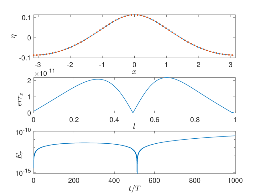
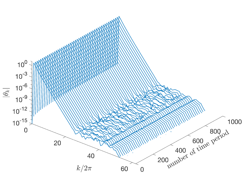
In Fig. 2(b), we plot the spectrum of . One can clearly see that there is no spurious growth in high-wave number region.
5.1.2 Wave breaking
To simulate wave breaking, we choose a travelling wave solution and amplify its profile by a factor . This is implemented by performing the following operations
Instead of using the Fourier filter, a -point smoothing formula invented in [10] turns out to be more robust when wave breaking happens. In Fig. 3, a travelling wave solution having unit water depth with crest-to-trough amplitude and wave number is amplified by factor and set to be the initial condition. Time step .
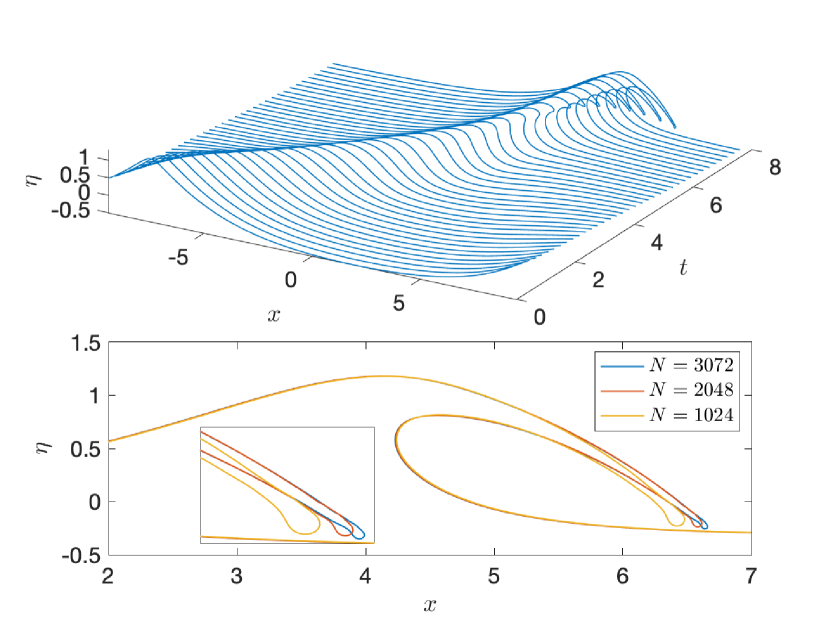
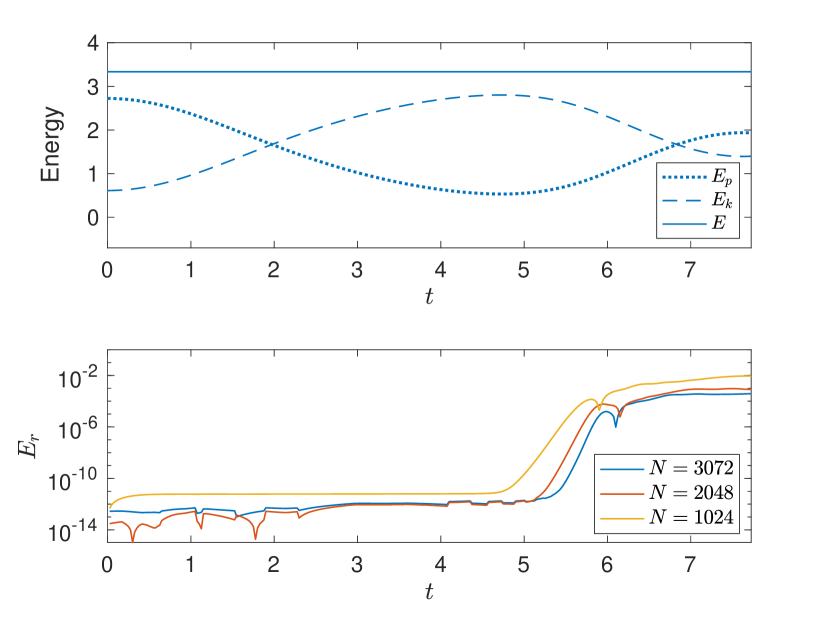
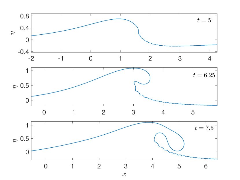
At the initial stage, gravitational potential energy is transferred to kinematic energy , resulting an accelerating moving front. At , the wave develops a vertical tangent and then becomes overhanging. A plunging breaker appears and becomes sharp at its tip. At , the wave becomes almost self-touching and encloses an air bubble on its front face. The nipple of the breaker has a locally round shape and tiny wiggles, which probably come from numerical oscillations due to the drastic increase of curvature. Higher resolutions are used to show that a gradually convergent solution can be obtained. A comparison of the wave profile at with and is plotted on the bottom of Fig. 3(a). The total energy is shown to be a constant between and . At , the kinetic energy and gravitational potential energy reach their extremums. Shortly after that, wave becomes overturned and the relative energy error increases rapidly, as shown in Fig. 3(b). When and , the upper bounds of are and and respectively, showing a convergent behaviour of solution. On the other hand, it is found that the wave breaking process can be significantly influenced by capillary effect, which generates small-scale ripples, known as parasitic waves. Surface tension effect, measured by the Bond number , can modify the characteristics of breakers, stabilize, and even suppress the breaking process. In Fig. 3(c) and (d), we perform simulations using the same initial condition as the previous one with the Bond number and . They represent relatively weak and strong surface tension effects. When , a large-scale plunging breaker is ultimately generated. However, the jet becomes larger and the tip is more round compared with gravitational plunging breaker. When , capillary effect is strong enough to suppress the formation of jet although a small overhanging structure is observed. In the end of simulation, we observe a closed air bubble, having a profile similar to the Crapper waves. This is typical for spilling breakers which characterize air entrainment and bubbles [8].
5.1.3 Head-on collision of solitary waves
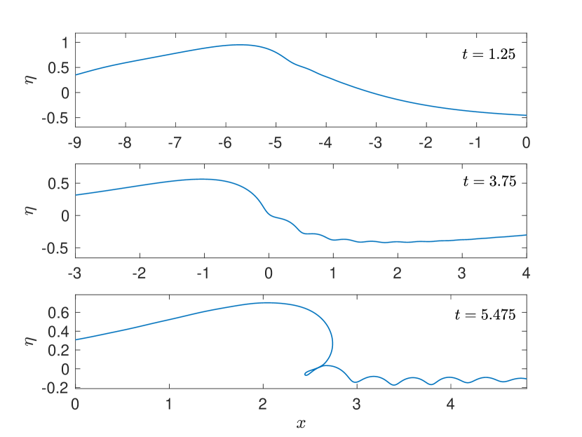
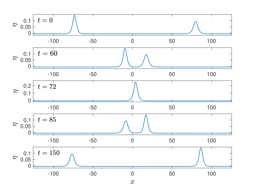
In Fig. 4, we exhibit a simulation of head-on collision of two solitary waves. Setting , we can simulate solitary waves by using long periodic waves. The initial condition is a superposition of two well-separated solitary waves with amplitude and opposite travelling direction. In the simulation, we choose , , and apply the th-order Fourier filter. The profiles at , and are shown in Fig. 4(a). As expected, the two solitary waves maintain their shape after collision, and radiate some tiny wave trains on their rear faces. A local illustration of the collision process is shown in Fig. 4(b). During the simulation, the energy error is well controlled and less than .
5.2 Interfacial gravity-capillary solitary waves
5.2.1 Bifurcations and profiles
It is well-known that the envelop of small-amplitude interfacial gravity-capillary solitary waves satisfies the NLS equation [16]
| (100) |
with
| (101) |
where is defined in (14). There exists a critical density ratio . When , the NLS equation is of the focussing type and has localised solitary wave solutions bifurcating from infinitesimal periodic waves. When , the NLS equation is of the defocusing type and only has non-localised dark soliton solutions. However, solitary waves of Euler equations have been found even when the corresponding NLS equation is of the defocusing type [16]. These solitary waves can only exist with finite amplitude, thus have no contradiction to the weakly nonlinear theory. Similar situation is also encountered in hydroelastic waves which model the motion of ice sheet [19]. Recent studies have shown that when , solitary waves evolve from the dark solitons or the generalised solitary waves, which themselves bifurcate from periodic waves [19, 29]. In this section, we focus on the stability of solitary waves and leave the dark solitons in future studies.
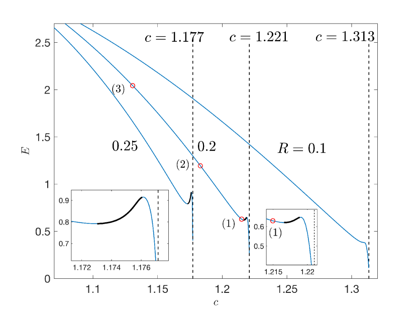
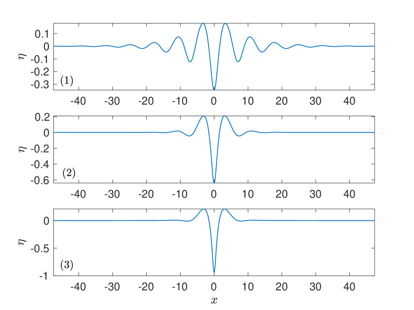
In Fig. 5 (a), we plot three speed-energy bifurcations of depression solitary waves with and . They belong to the case . Therefore, solitary waves bifurcate from infinitesimal periodic waves at the minimum phase speed . At small amplitude, they have wave-packet profiles with spatially decaying tails in the far field. When wave amplitude increases, the wave speed decreases monotonically. We display three typical waves with in Fig. 5 (b). Ultimately, only one single trough at the center survives and keeps steepening until an overhanging structure develops. The limiting configuration of the depression solitary waves is a self-intersecting wave with a closed fluid bubble at the trough, similar to the famous Crapper waves locally [7].
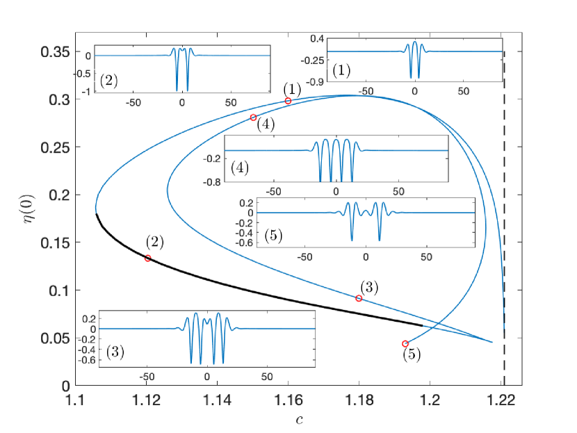
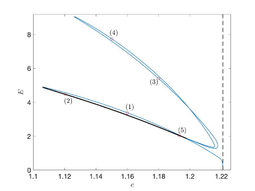
On the other hand, the evolution of elevation solitary waves is more complicated. In Fig. 6 (a), we plot the speed-amplitude bifurcation curve of , as well as five typical waves. In Fig. 6 (b), we plot the corresponding speed-energy curve. Close to the bifurcation point , elevation solitary waves feature wave-packet profiles with positive values of at the center. When the wave amplitude increases, wave speed decreases monotonically until the first turning point appears. Depression solitary waves then gradually develop more troughs and peaks following the bifurcation . After passing through four turning points, they resemble two side-by-side depression waves. Readers who are interested in the global bifurcation structure are referred to [9] for details.
5.2.2 Linear stability
Using the new formulation described in section 4.3.2, we perform linear stability analysis to solitary waves with . As shown in Fig. 5, the energy curve of the depression solitary waves undergoes two stationary points. According to [24], this implies that exchange of stability could happen at these points. Indeed, we found that depression solitary waves are linearly stable except the those solutions between the two stationary points. The linearly unstable solutions are represented by the black solid lines in Fig. 5 (a). This is different from the case , i.e. depression gravity-capillary solitary waves of surface type, which have a monotonic energy curve and are linearly stable no matter their amplitude.
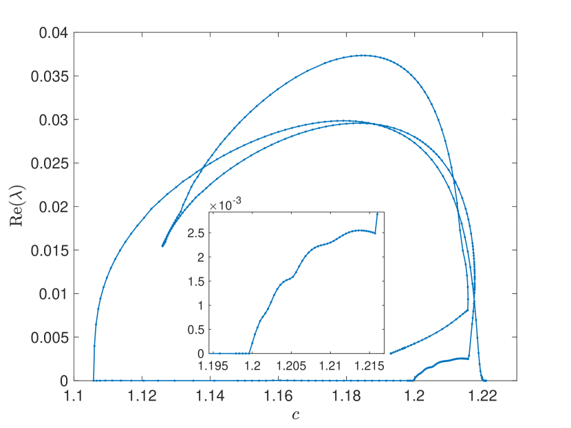
For elevation solitary waves, on the other hand, small-amplitude solutions are linearly unstable. As there exist multiple stationary points on the energy curve, the first exchange of stability is found at . Solutions then becomes linearly stable until , as shown in Fig. 6. Surprisingly, this is not a stationary point of energy. In fact, what happens there is a dominant superharmonic instability instead of the excahnge of stability. The difference between the two concepts is that the former has nonzero imaginary part of growth rate, i.e. , while the latter has zero imaginary part of growth rate. The linear growth rate is plotted in Fig.7(a). At , i.e. the second stationary point of energy, an exchange of stability happens and replaces the superharmonic instability, which is manifested by the sharp angle of the curve. When , i.e. surface gravity-capillary solitary waves, we also observe that the superharmonic instability emerges and dominates before the second stationary point appears.
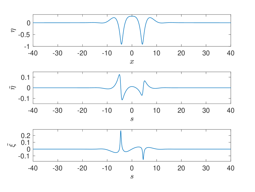
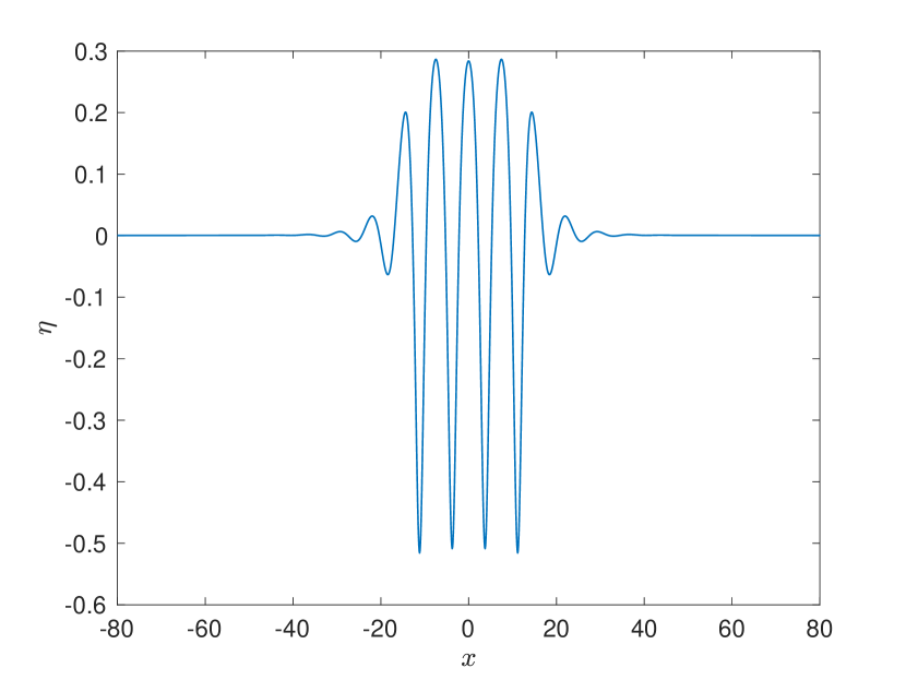
In Fig. 7(b), a linearly unstable elevation solitary wave with wave speed and wave height is plotted, as well as its most unstable modes for and . By setting , and , we get the growth rate , and respectively.
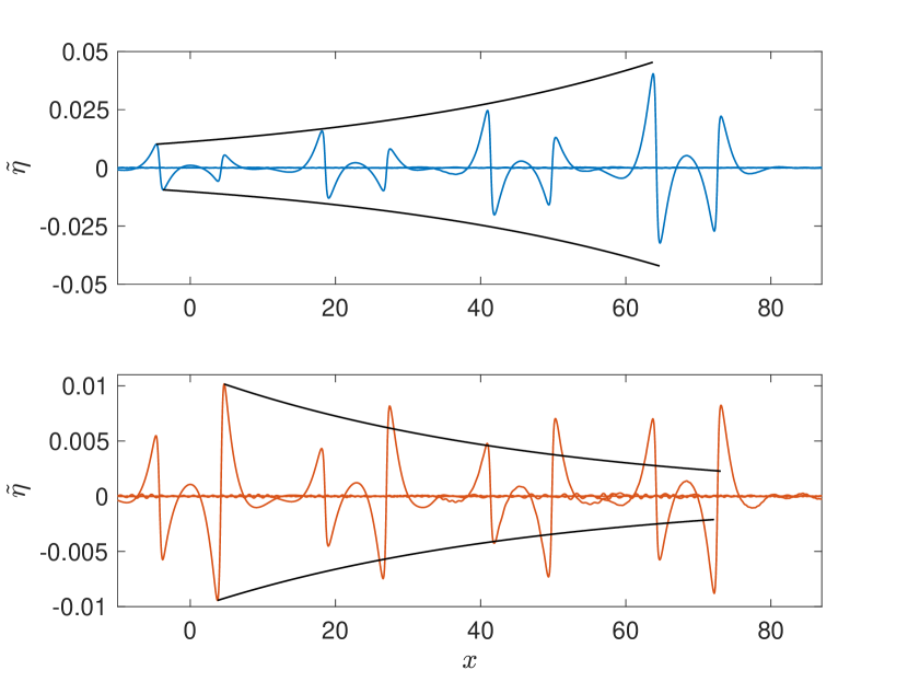
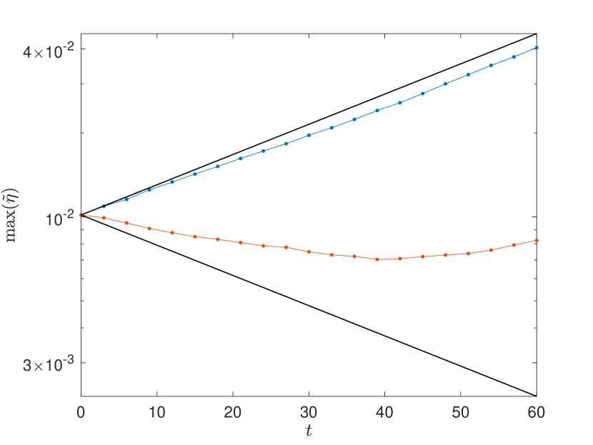
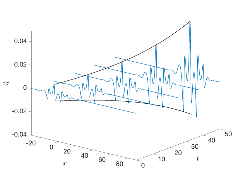
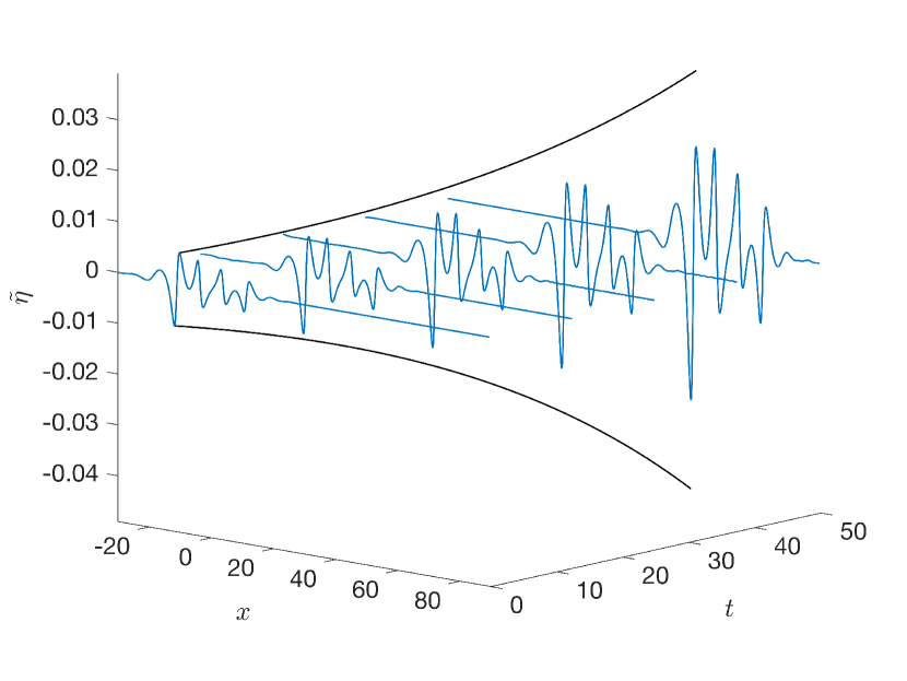
To verify the linear stability theory, we perform fully nonlinear simulation for this solution. The solitary wave is superposed a small perturbation which is proportional to the most unstable mode and then set to be the initial condition. The evolution of the disturbance is plotted on the top of Fig. 8 (a). The profiles from left to right correspond to , and . The prediction from linear stability analysis is shown by the black curve, which represents the envelope of and exhibits good agreement to the fully nonlinear simulation. It is interesting to note that there exists a linearly stable mode whose growth rate equals to . On the bottom of Fig. 8 (a), we show the time evolution of this mode when it is superposed to the solitary wave as perturbatoin. Profiles of are plotted at , and from left to right. Initially decreases roughly following the prediction of linear stability until after the disturbance starts to grow. The growth rate of the two modes based on fully nonlinear calculation and linear stability theory are shown in Fig. 8 (b). Initially, linear stability theory predicts the growth rate of the most unstable mode quite well, but slightly overestimates it later. For the linearly stable mode, however, linear theory does not give a very good estimation.
When the exchange of stability happens, solutions can have more than one unstable modes. In Fig. 9 (a), we display a solitary wave with and . It is located on the linearly unstable branch after passing through three stationary points of energy and found to have three unstable modes, whose corresponding -profiles are plotted in Fig. 9(b). From top to bottom, their growth rates are , and respectively. In Fig. 10, we shown the evolution of the perturbation which is initially set to be proportional to the most unstable mode (left) and the second most unstable mode (right). The black curves are the envelopes of calculated from linear stability analysis. It is clear that linear theory gives an excellent estimation for the most unstable mode but overestimates the growth rate of the second most unstable mode.

5.2.3 Head-on collision
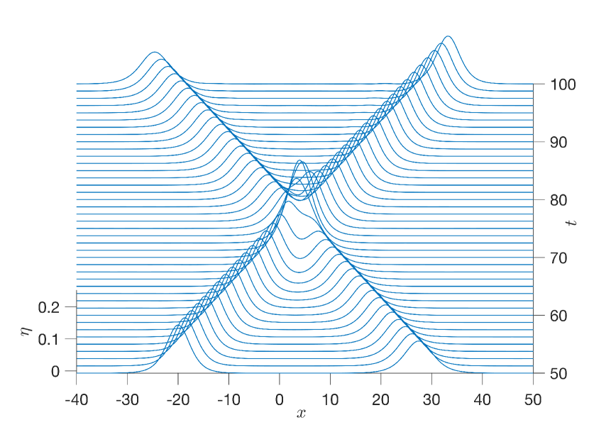
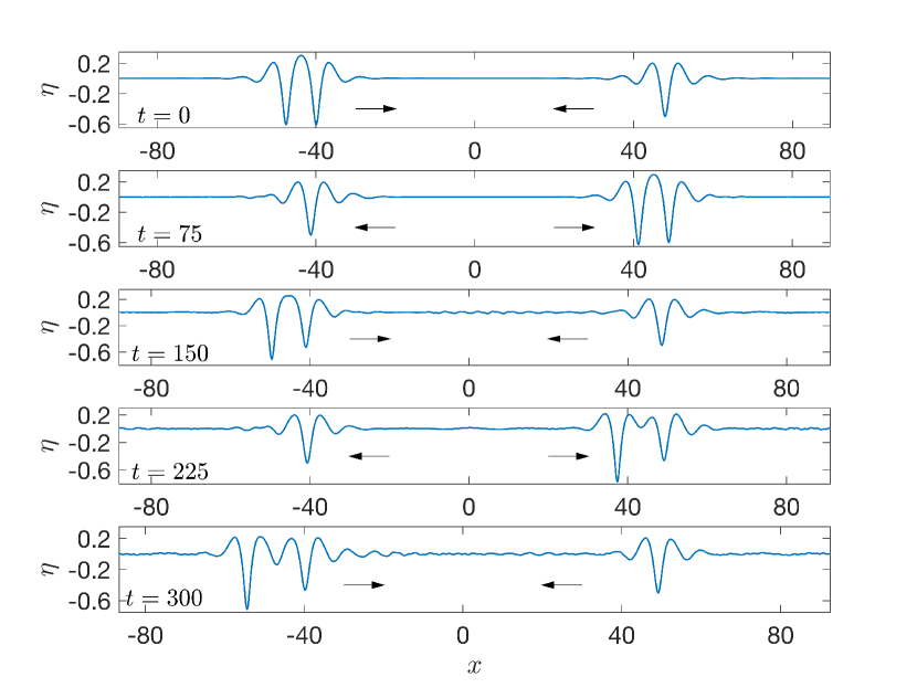
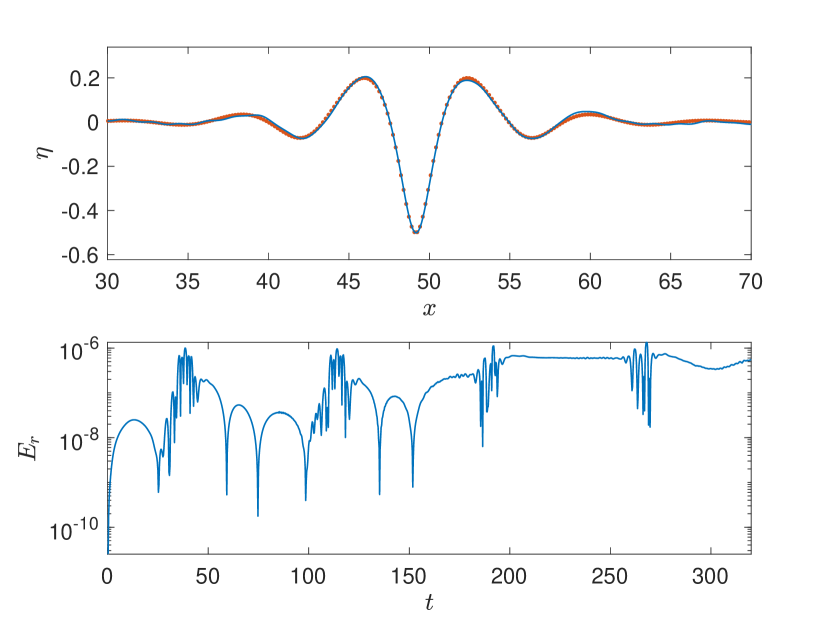
We further check the stability of solitary waves by simulating their head-on collisions. In Fig. 11, we choose two well-separated solitary waves as the initial condition of fully nonlinear simulation. One of them is of the depression type () and linearly stable, the other one is of the elevation type () and linearly unstable. We set and . Since we impose periodic boundary conditions, the two solitary waves can keep colliding during simulation. In Fig. 11, we plot the initial profile () and other four typical profiles at , and . The depression solitary wave is rather robust and maintains its shape after four collisions. This can be clearly seen from a comparison between its initial profile and the profile at , which is shown on the top of Fig. 11(a). The two profiles are almost indistinguishable except the tiny difference due to the radiated disturbances. On the other hand, the elevation solitary wave gradually loses its symmetry after two collisions with a manifestation that its two troughs have different heights. After the fourth collision, the elevation solitary wave undergoes complete distortion and begins to decompose into two side-by-side depression solitary waves. During the simulation, the energy error is well controlled and less than . This is shown on the bottom of Fig. 11(a).
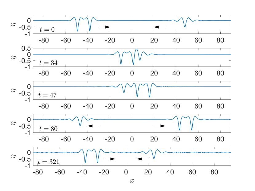
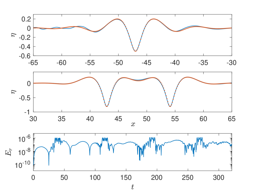
In Fig. 12, we display another simulation of head-on collisions between a depression solitary wave () and an elevation solitary wave (). Both waves are linearly stable according to linear stability analysis. We set and . The initial condition is shown on the top of Fig. 12. The profiles at , and show the process of the first collision and the separation later. Simulation continues until the fourth collision occurs. As expected, both solitary waves are rather robust and maintain their shape after collisions, as can be seen from Fig. 12 where the comparisons of their wave profiles are presented. There is only tiny difference between the initial profiles and the profiles at for both solitary waves. On the bottom of Fig. 12 (b), we plot the energy error which is less the during the simulation.
5.3 Vortex roll-up
Small-amplitude interfacial waves are neutrally stable according to the dispersion relation (14). When there is a background shear across the interface, however, K-H instability will be triggered and generate the vortex roll-up structure [13]. Considering two uniform background currents and in the lower and upper layer, we have the following linear solutions
| (102) | ||||
| (103) | ||||
| (104) |
where has two complex roots given and
| (105) |
The critical condition to trigger the K-H instability is
| (106) |
Thus the shear must be strong enough to satisfy
| (107) |
Taking , we can replace the variable by in Eqs. (102)-(104). Thus we can choose the following initial condition for our simulations
| (108) | ||||
| (109) |
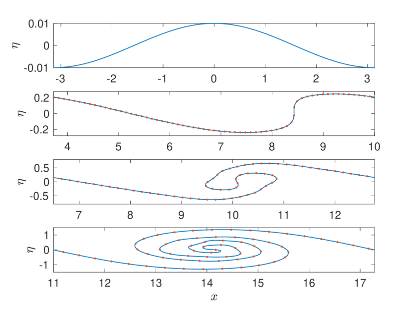
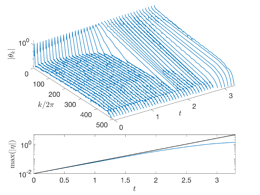
Fig. 13(a) displays a simulation of the vortex roll-up structure at different moments. We set , , and choose the unstable root . The interface grows quickly in amplitude and follows the linear theory closely. At it develops a vertical tangent. After that, the interface rolls over and forms two spiral fingers and grows in length. Close to the tip of these fingers, there is trace of small-amplitude wiggles due to the surface tension effect. This has also been previously observed and reported in [13, 3]. At , the interface develops a standard vortex roll-up structure of the K-H type. As time progresses, the interface spirals, eventually leading to self-intersection, as reported in [13]. On the top of Fig. 13(b), we plot the spectrum of to show the effectiveness of the th-order Fourier filter in suppressing the aliasing error. The bottom figure illustrates max against from both the fully nonlinear simulation (blue curve) and the linear theory (black curve). These curves closely align in a logarithmic scale until .
6 Conclusions
In this paper, we present a novel boundary-integral method designed to simulate nonlinear two-dimensional unsteady interfacial waves and surface waves. The essential parts of the method are: (1) parameterizing the interface or surface by using their physical arclength, (2) establishing the Eulerian or mixed Eulerian-Lagrangian description, (3) using Cauchy’s integral formula for solving the Laplace equation, and (4) employing the formulation to integrate in time and construct the interface. The advantages of our algorithm are due to the intrinsic dimension-reducing nature of the boundary-integral method, the numerical efficiency of the formulation, and the uniform distribution of sample points on the interface or surface. We are able to simulate various highly nonlinear wave motions, such as large-scale wave breaking, collisions of solitary waves, vortex roll-up structures due to the K-H instability, etc. We find that our algorithm possesses excellent numerical accuracy and robustness, making it very suitable for long-term simulations.
Particularly, we focus on the stability of symmetric interfacial gravity-capillary solitary waves in deep water. We calculate the depression and elevation solitary waves by using the Newton-Krylov method which can speed up the computation significantly. Previous studies on surface gravity-capillary solitary waves have shown that the depression waves are always stable. On the other hand, the elevation waves are unstable except those solutions between the first and the second stationary points on the energy curve. We reformulate the previous linear stability analysis and derive a new formulation suitable for interfacial waves. It possesses both numerical efficiency and robustness. This new formulation is employed to a special case with and yields that interfacial solitary waves have very similar stability properties to their counterpart of surface type. However, the energy curve of the depression solitary waves is not monotonic, resulting in exchanges of stability at the stationary points. Therefore, the depression solitary waves are linearly stable except a little part of them between the two stationary points of energy. For the elevation solitary waves, they are linearly unstable in small amplitude but turn to be stable after the first energy stationary point. We find that before the appearance of the second stationary point, elevation solitary waves are detected instability, which is a dominant superharmonic instability. At the second stationary point of energy, the exchange of stability happens again and solutions are linearly unstable thereafter. These findings are confirmed by our fully nonlinear simulations of solitary waves, especially their head-on collisions.
Acknowledgements
X.G. would like to acknowledge the support from the Chinese Scholarship Council (no. 202004910418).
Appendix A Derivation of Eqs. (17) and (21)
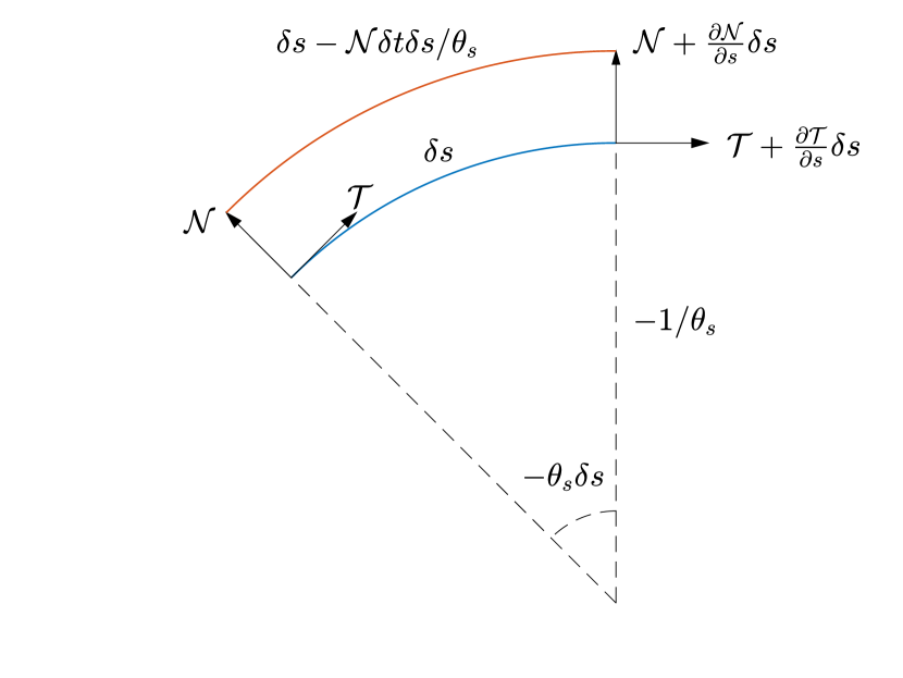
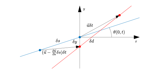
In Fig. 14(a), we show an infinitesimal surface element with length and curvature . The increment of its length in time consists of the contribution of the tangential velocity and the normal velocity . The former stretches the element and generates an quantity . The normal velocity gives rise to an expansion effect, causing a quantity in leading order. Note that the minus sign is due to the fact that is our schematic. Putting these terms together, we have
| (110) |
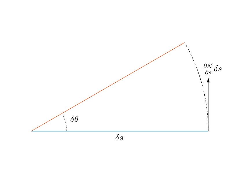
Similarly, the increment of inclination angle also comes from the contribution of and . The former gives the element a translation in direction, which causes a quantity . The normal velocity generates a local rotation with angle (see Fig. 14 (b)). Thus we have
| (111) |
Appendix B Derivation of in Case II
Fig. 15 shows a local schematic of an interface and two Lagrangian particles on it at time (blue) and (red). Initially, the distance between the two particles is and the right one is located on the left boundary of the computational domain, which is set to be the the -axis without loss of generality. In time, the left particle moves to the boundary. According (19)
| (112) |
where is the distance between the two red points. Using the geometric relation, we have
| (113) |
The minus sign of is due to the fact that we define as the vertical component of the vector starting from the blue point and pointing to the red point on the -axis, which is negative in the schematic.
References
- [1] G. R. Baker. Generalized vortex methods for free-surface flows. In Waves on fluid interfaces, pages 53–81. Elsevier, 1983.
- [2] G. R. Baker, D. I. Meiron, and S. A. Orszag. Vortex simulations of the rayleigh–taylor instability. Phys. Fluids, 23(8):1485–1490, 1980.
- [3] G. R. Baker and A. Nachbin. Stable methods for vortex sheet motion in the presence of surface tension. SIAM J. Sci. Comput, 19(5):1737–1766, 1998.
- [4] T. B. Benjamin and T. J. Bridges. Reappraisal of the kelvin–helmholtz problem. part 1. Hamiltonian structure. J. Fluid Mech., 333:301–325, 1997.
- [5] D. C. Calvo and T. R. Akylas. Stability of steep gravity–capillary solitary waves in deep water. J. Fluid Mech., 452:123–143, 2002.
- [6] D. C. Calvo and T. R. Akylas. On interfacial gravity-capillary solitary waves of the benjamin type and their stability. Phys. Fluids, 15(5):1261–1270, 2003.
- [7] G. D. Crapper. An exact solution for progressive capillary waves of arbitrary amplitude. J. Fluid Mech., 2(6):532–540, 1957.
- [8] L. Deike, S. Popinet, and W. K. Melville. Capillary effects on wave breaking. J. Fluid Mech., 769:541–569, 2015.
- [9] A. Doak, T. Gao, and J.-M. Vanden-Broeck. Global bifurcation of capillary-gravity dark solitary waves on the surface of a conducting fluid under normal electric fields. Quart. J. Mech. Appl. Math., 75(3):215–234, 2022.
- [10] J. W. Dold. An efficient surface-integral algorithm applied to unsteady gravity waves. J. Comput. Phys., 103(1):90–115, 1992.
- [11] J. Grue, H. A. Friis, E. Palm, and P. O. Rusaas. A method for computing unsteady fully nonlinear interfacial waves. J. Fluid Mech., 351:223–252, 1997.
- [12] T. Y. Hou and R. Li. Computing nearly singular solutions using pseudo-spectral methods. J. Comput. Phys., 226(1):379–397, 2007.
- [13] T. Y. Hou, J. S. Lowengrub, and M. J. Shelley. Removing the stiffness from interfacial flows with surface tension. J. Comput. Phys., 114(2):312–338, 1994.
- [14] T. Y. Hou, J. S. Lowengrub, and M. J. Shelley. Boundary integral methods for multicomponent fluids and multiphase materials. J. Comput. Phys., 169(2):302–362, 2001.
- [15] D. A. Knoll and D. E. Keyes. Jacobian-free newton–krylov methods: a survey of approaches and applications. J. Comput. Phys., 193(2):357–397, 2004.
- [16] O. Laget and F. Dias. Numerical computation of capillary–gravity interfacial solitary waves. J. Fluid Mech., 349:221–251, 1997.
- [17] M. S. Longuet-Higgins and E. D. Cokelet. The deformation of steep surface waves on water-i. a numerical method of computation. Proc. R. Soc. London A, 350(1660):1–26, 1976.
- [18] P. A. Milewski, J.-M. Vanden-Broeck, and Z. Wang. Dynamics of steep two-dimensional gravity–capillary solitary waves. J. Fluid Mech., 664:466–477, 2010.
- [19] P. A. Milewski, J.-M. Vanden-Broeck, and Z. Wang. Hydroelastic solitary waves in deep water. J. Fluid Mech., 679:628–640, 2011.
- [20] S. Murashige and W. Choi. A numerical study on parasitic capillary waves using unsteady conformal mapping. J. Comput. Phys., 328:234–257, 2017.
- [21] R. Pethiyagoda, S. W. McCue, T. J. Moroney, and J. M. Back. Jacobian-free newton–krylov methods with gpu acceleration for computing nonlinear ship wave patterns. J. Comput. Phys., 269:297–313, 2014.
- [22] D. I. Pullin. Numerical studies of surface-tension effects in nonlinear kelvin–helmholtz and rayleigh–taylor instability. J. Fluid Mech., 119:507–532, 1982.
- [23] R. Ribeiro, P. A. Milewski, and A. Nachbin. Flow structure beneath rotational water waves with stagnation points. J. Fluid Mech., 812:792–814, 2017.
- [24] P. G. Saffman. The superharmonic instability of finite-amplitude water waves. J. Fluid Mech., 159:169–174, 1985.
- [25] M. Tanaka. The stability of solitary waves. Phys. Fluids, 29(3):650–655, 1986.
- [26] L. N. Trefethen and D. Bau. Numerical linear algebra, volume 181. SIAM, 2022.
- [27] C. Ţugulan, O. Trichtchenko, and E. Părău. Three-dimensional waves under ice computed with novel preconditioning methods. J. Comput. Phys., 459:111129, 2022.
- [28] Z. Wang. Stability and dynamics of two-dimensional fully nonlinear gravity–capillary solitary waves in deep water. J. Fluid Mech., 809:530–552, 2016.
- [29] Z. Wang, J.-M. Vanden-Broeck, and H. Meng. A quasi-planar model for gravity-capillary interfacial waves in deep water. Stud. Appl. Math., 133(2):232–256, 2014.
- [30] Y. Yang. The initial value problem of a rising bubble in a two-dimensional vertical channel. Phys. Fluids, 4(5):913–920, 1992.
- [31] V. E. Zakharov. Stability of periodic waves of finite amplitude on the surface of a deep fluid. J. Appl. Mech. Tech. Phys., 9(2):190–194, 1968.