Electron-tunneling-induced thermoelectric effects

Abstract

We introduce a direct (Seebeck) and inverse (Peltier) thermolectric effect induced by electron tunneling between closely separated conducting films. When a transverse temperature gradient is applied along one of two films, a bias voltage is induced in the second thanks to the heat transfer mediated by electrons tunneling through the separation gap. We highlight a non trivial behavior for this Seebeck effect with respect to geometric characteristics of interacting films. Conversely, when an electric current passes through one of two films a strong thermal power can be removed from or inserted in the second film through an induced Peltier effect. In particular we highlight conditions where the induced Seebeck and Peltier coefficients are larger than in the bulk. These induced thermoelectric effects could find broad applications in the fields of energy conversion and cooling at nanoscale.

Thermoelectric effects are the direct conversion of the temperature difference inside a material into a bias voltage (Seebeck effect) and the conversion of an electric current flowing through this material into a negative or positive thermal power (Peltier effect). The efficiency of a thermoelectric system can be evaluated with the figure of merit $ZT$ of material which is defined as $ZT=\frac{S_{0}^{2}\kappa_{e}T}{\kappa_{T}}$, where $T$ is the temperature, $S_{0}=-\Delta\phi/\Delta T$ is the Seebeck coefficient which quantify the voltage $\Delta\phi$ generated under a temperature difference $\Delta T$, $\kappa_{e}$ and $\kappa_{T}$ denoting the electrical and thermal conductivity of material, respectively. Recent works Majumdar ; Rodgers have been performed using nanomaterials or nanocomposite structures to increase the $ZT$ by reducing the thermal conductivity while keeping its electric counterpart constant.

In this Letter we introduce thermoelectric effects induced by the tunneling of electrons between two coupled conductors separated by a small gap. When the size of this gap is sufficiently small and a temperature difference is applied along one of two conductors, a spatially varying density of free charges can be induced across the gap by tunneling effect giving rise to a drift and a diffusion current into the second conductor. On the opposite, when a bias voltage is applied along one of the conductors, a heat flux can be extracted from or inserted into the second conductor. We develop a general theory to describe these thermoelectric effects between two metallic films and analyze its main characteristics with respect to the separation gap and films thicknesses.

To start let us consider the system sketched in Fig. 1 made of two conducting films of same thickness $t_{z}$, length $L$ and width $t_{y}$, separated by a vacuum gap of thickness $d$.

Figure 1: Sketch of two conducting films separated by a vacuum gap, coupled via near-field radiative heat exchanges and electron tunneling. (a) Induced Seebeck effect: the top film is connected to two thermal reservoirs at temperatures $T_{1}(0)$ and $T_{1}(L)$, giving rise to a temperature gradient. It is grounded on its left side [$\phi_{1}(0)=0$] and no current can escape from its right side [$J_{1}(L)=0$]. The electric current $J_{2}$ induced in the second film (having adiabatic thermal conditions $\Phi_{2}(0)=\Phi_{2}(L)=0$) can be measured with an ammeter of resistance $R$. (b) Induced Peltier effect: a bias voltage $\Delta\phi_{1}$ is applied along the top film while it is connected on its two ends to two reservoirs of same temperature $T_{1}(0)=T_{1}(L)$. The second film is electrically insulated on its two sides [$J_{2}(0)=J_{2}(L)=0$] and adiabatic conditions are applied on its right side [$\Phi_{2}(L)=0$] while its left side is connected to a thermal reservoir. The bias voltage induces a thermal power $\Phi_{2}(0)$ which can enter of leave the film on its left side.

We assume that along each film ($i=1,2$) small temperature and chemical potential differences $\Delta T_{i}=T_{i}(L)-T_{i}(0)$ and $\Delta\mu_{i}=\mu_{i}(L)-\mu_{i}(0)$ are applied. Then, according to the Onsager theory de Groot , the local particle current densities $\mathcal{J}_{i}^{(\rm P)}(x)$ and energy fluxes $\mathcal{J}_{i}^{(\rm E)}(x)$ along each film are linearly related to the thermodynamic forces $\mathcal{F}_{i}^{\rm(P)}=\frac{\mathrm{d}}{\mathrm{d}x}(\frac{-\mu_{i}(x)}{T_{i}(x)})$ and $\mathcal{F}_{i}^{\rm(E)}=\frac{\mathrm{d}}{\mathrm{d}x}(\frac{1}{T_{i}(x)})$ by the relations

$$\left(\begin{array}[]{c}\mathcal{J}_{i}^{(\rm P)}(x)\\ \mathcal{J}_{i}^{(\rm E)}(x)\end{array}\right)=\left(\begin{array}[]{cc}L_{i}^{\rm(PP)}&L_{i}^{\rm(PE)}\\ L_{i}^{\rm(EP)}&L_{i}^{\rm(EE)}\end{array}\right)\left(\begin{array}[]{c}\mathcal{F}_{i}^{\rm(p)}(x)\\ \mathcal{F}_{i}^{\rm(E)}(x)\end{array}\right),$$ (1)

where $L_{i}^{(ab)}$ $(a,b=\mathrm{P},\mathrm{E})$ are the Onsager coefficients which are related to the familiar transport coefficients. Onsager equations can be rewritten in terms of the electric current densities $J_{i}(x)=-e\mathcal{J}^{\rm(P)}_{i}(x)$ ($-e$ is the electron charge) and heat fluxes $\Phi_{i}(x)=\mathcal{J}^{\rm(E)}_{i}(x)-\mu(x)\mathcal{J}^{\rm(p)}_{i}(x)$, and in terms of temperature and bias voltage $\phi_{i}(x)=-\mu_{i}(x)/e$ gradients, given by pottier

$$\left(\begin{array}[]{c}J_{i}(x)\\ \Phi_{i}(x)\end{array}\right)=\frac{\kappa_{T}}{\Lambda}\left(\begin{array}[]{cc}1/T_{i}(x)&S_{0}/T_{i}(x)\\ S_{0}&\Lambda+S_{0}^{2}\end{array}\right)\left(\begin{array}[]{c}-\phi_{i}^{\prime}(x)\\ -T_{i}^{\prime}(x)\end{array}\right),$$ (2)

where we used Ohm’s law $J_{i}(x)=-\kappa_{e}\phi_{i}^{\prime}(x)$ (at constant temperature), the Seebeck relation, Fourier’s law $\Phi_{i}(x)=-\kappa_{T}T_{i}^{\prime}(x)$ (at zero current), and Wiedemann-Franz’s law $\kappa_{e}/\kappa_{T}=\Lambda T_{i}(x)$ ($\Lambda=\pi^{2}k^{2}_{\rm B}/3e^{2}$ is the Lorenz number, $k_{\rm B}$ Boltzmann’s constant), in order to write the equations in terms of $S_{0}$ and $\kappa_{T}$ whose dependence on temperature and bias is negligible for conducting elements near ambient temperatures firstprinciples .

The two films exchange heat by thermal radiation and close to the contact electrons can tunnel through the separation gap carrying both charge and heat. In steady-state regime, the corresponding energy and charge conservation equations for a given volume element (of each body $i=1,2$) read

$$\begin{split}-t_{z}\Phi_{i}^{\prime}(x)+(-1)^{i}\Phi^{\rm(rad)}(x)+\Phi^{\rm(el)}_{i}(x)&=0,\\ -t_{z}J_{i}^{\prime}(x)+(-1)^{i}J^{\rm(tun)}(x)&=0.\\ \end{split}$$ (3)

The tunneling current density $J^{\rm(tun)}(x)$ reads Simmons

$$J^{\rm(tun)}(x) =\frac{em_{e}}{2\pi^{2}\hbar^{3}}\int_{\tilde{E}(x)}^{\infty}\mathrm{d}E_{z}\int_{0}^{\infty}\mathrm{d}E_{\perp}$$ (4)

$$\times\Delta n_{\rm FD}(E,T_{1}(x),T_{2}(x),\mu_{1}(x),\mu_{2}(x))\mathcal{T}^{\rm(el)}(E_{z}),$$

where $m_{e}$ is the electron mass, $E=E_{\perp}+E_{z}$ its total kinetic energy decomposed in contributions stemming from velocities perpendicular and parallel to the exchange surface, the bottom of the integral goes from the bottom of the local band $\tilde{E}(x)=\mathrm{max}\{0,-e[\phi_{2}(x)-\phi_{1}(x)]\}$, and $\Delta n_{\rm FD}$ is the difference of Fermi-Dirac distributions, depending on both local temperature $T_{i}$ and local chemical potential $\mu_{i}$ associated with each medium. In Eq. (4) $\mathcal{T}^{\rm(el)}(E_{z})$ is the electronic transmission probability through the separation gap which can be calculated using the semiclassical Wentzel-Kramers-Brillouin method WKB or more elaborated methods Mauricio .

Electrons tunneling gives rise to a heat transfer which takes the form Xu ; Mauricio2

$$\Phi_{i}^{(\mathrm{el})}(T_{1},T_{2},d,x)=(-1)^{i}\frac{m_{e}}{2\pi^{2}\hbar^{3}}\int_{\tilde{E}}^{\infty}\mathrm{d}E_{z}\int_{0}^{\infty}\mathrm{d}E_{\perp}$$ (5)

$$\times(E-\mu_{i}(x))\Delta n_{\rm FD}(E,T_{1}(x),T_{2}(x),\mu_{1}(x),\mu_{2}(x)\mathcal{T}^{\rm(el)}(E_{z}).$$

The flux carried by photons, evaluated from fluctuational-electrodynamics theory Polder , reads

$$\Phi^{\text{(rad)}}(x)= \underset{l=\mathrm{s},\mathrm{p}}{\sum}\int_{0}^{\infty}\!\frac{d\omega}{2\pi}\ \hbar\omega\Delta n_{\rm BE}(T_{1}(x),T_{2}(x))$$ (6)

$$\times\int_{0}^{\infty}\frac{d\kappa}{2\pi}\kappa\,\mathcal{T}_{l}^{\text{(rad)}}(\omega,\kappa),$$

where $\mathcal{T}_{l}^{\text{(rad)}}(\omega,\kappa)$ denotes the energy transmission coefficient for one electromagnetic mode $(\omega,\kappa)$ for the polarizations $l=\mathrm{s},\mathrm{p}$ and $n_{\rm BE}(\omega,T)=1/[\exp(\hbar\omega/k_{\rm B}T)-1]$ is the Bose-Einstein distribution function.

To analyze the thermoelectric effects induced by electron tunneling we solve the nonlinear system of Eqs. (2) and (3) with respect to the temperatures $T_{i}(x)$ and bias voltage $\phi_{i}(x)$ profiles in the case of two complementary scenarios, corresponding to suitable configurations where the direct (Seebeck) and inverse (Peltier) thermoelectric effects can be observed. To this end, we first replace the expression of tunnel current by its linearized form in terms of both $T_{i}(x)$ and $\phi_{i}(x)$, which yields

$$J^{\rm(tun)}(x)\approx G_{J}(d)[\phi_{1}(x)-\phi_{2}(x)]-h_{J}(d)[T_{1}(x)-T_{2}(x)],$$ (7)

where $G_{J}$ and $h_{J}$ denote, respectively, the electrical and thermal tunneling conductances (per unit surface) that depend only on the gap thickness $d$. On the other hand, the heat fluxes must be expanded to the quadratic order

$$\begin{split}\Phi^{\rm(el)}_{1}(x)&\simeq G_{\Phi}(d)[\phi_{1}(x)-\phi_{2}(x)]+\frac{G_{J}(d)}{2}[\phi_{1}(x)-\phi_{2}(x)]^{2}\\ &-h_{\Phi}(d)[T_{1}(x)-T_{2}(x)]-\tilde{h}_{\Phi}(d)[T_{1}(x)-T_{2}(x)]^{2}\\ &-\frac{h_{J}(d)}{2}[\phi_{1}(x)-\phi_{2}(x)][T_{1}(x)-T_{2}(x)]\\ \Phi^{\rm(el)}_{2}(x)&\simeq-G_{\Phi}(d)[\phi_{1}(x)-\phi_{2}(x)]+\frac{G_{J}(d)}{2}[\phi_{1}(x)-\phi_{2}(x)]^{2}\\ &+h_{\Phi}(d)(T_{1}-T_{2})+\tilde{h}_{\Phi}(d)[T_{1}(x)-T_{2}(x)]^{2}\\ &-\frac{h_{J}(d)}{2}[\phi_{1}(x)-\phi_{2}(x)][T_{1}(x)-T_{2}(x)],\end{split}$$ (8)

so that the tunneling current density can satisfy the energy conservation equation

$$\Phi_{1}^{\rm(el)}(x)+\Phi_{2}^{\rm(el)}(x)=J^{\rm(tun)}(x)[\phi_{1}(x)-\phi_{2}(x)].$$ (9)

The lhs in this expression corresponds to the thermal power mediated by electron tunneling through the separation gap while the rhs is the electric power associated to tunnel current. In Eq. (8), $G_{\Phi}(d)$, $h_{\Phi}(d)$ and $\tilde{h}_{\Phi}(d)$, are the thermal conductances and Hessian associated to the bias voltage and temperature differences. All parameters $G_{J},h_{J},G_{\Phi},h_{\Phi},\tilde{h}_{\Phi}$ can be fitted for any separation distance from the general expressions (4), (5) and (6).

In the first scenario, [see Fig. 1(a)], a primary temperature gradient is applied along body 1 [i.e. $T_{1}(0)=T_{0}$ and $T_{1}(L)=T_{0}+\Delta T$] and this body is electrically connected to the ground at $x=0$ [i.e. $\phi_{1}(0)=0$] and no electric current can escape from its opposite side [i.e. $J_{1}(L)=0$]. As for the second, we assume it is connected to an ammeter of resistance $R$ and a current is free to circulate through it thanks to the primary temperature gradient in body 1. Therefore, according to Ohm’s law, the bias voltage $\Delta\phi_{2}=\phi_{2}(L)-\phi_{2}(0)$ along body 2 satisfies $\Delta\phi_{2}=R\>J_{2}(L)\>t_{z}t_{y}$. We assume adiabatic conditions at both ends of body 2 [$\Phi_{2}(0)=\Phi_{2}(L)=0$] and continuity of the current through the resistance [i.e. $J_{2}(0)=J_{2}(L)$]. The differential system (3) associated with expressions (8) and (9) is solved numerically using a 4th order collocation method as described in Ref. diffequations . The induced electromotive force that develops in the second solid when a temperature gradient is applied in the first one can be quantified by the induced Seebeck coefficient, $S=-\Delta\phi_{2}/\Delta T_{1}$, directly proportional to the current $I_{2}(L)$ [$I_{i}(L)=J_{i}(L)t_{z}t_{y}$] via Ohm’s law.

The results are plotted in Fig. 2 for two gold films ($t_{y}=L$) as a function of their separation distance.

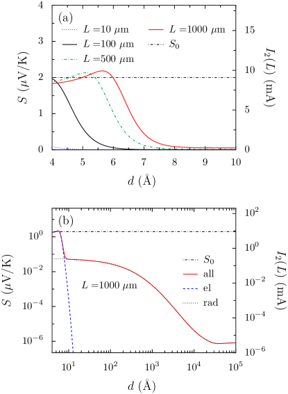
Figure 2: Induced Seebeck coefficient $S$ and induced current $I_{2}(L)$ as a function of the gap thickness $d$ between two gold films of thickness $t_{z}=5\>\mu$m. The first film is held at $T_{0}=300\;$K on its left end and a temperature difference $\Delta T=100\;$K is applied along it. The second film is connected to a resistance of $R=22\;$m$\Omega$. In (a) and (b) the Seebeck coefficient for bulk gold $S_{0}\approx 2\;\mu$m seebeckgold is represented by a dash-dotted line. In (a) the curves are plotted for various values of the system length $L$, in (b) for a large range of distances (red). In (b) the induced Seebeck coefficient due to the electronic contribution (blue dashed line) and the purely radiative contribution (black dotted) are also shown.

In Fig. 2(a) we see that the induced Seebeck coefficient increases at close separation distances (as a result of an increase tunneling of free charges), and also when the length of the system increases. It is worthwhile noting that for sufficiently long films, this coefficient can go beyond the bulk Seebeck coefficient $S_{0}$ [dash-dotted line in Fig. 2(a)]. In Fig. 2(b) we show the evolution of this effect at larger separation distances and highlight the relative contributions of different carriers. For distances larger than 1 nm the electronic contribution to the transfer falls down very rapidly and the coupling between the two films is manly due to, first, non-propagative thermal phonons (i.e. near-field radiative heat transfer) for separation distances smaller than the thermal wavelength and to propagative photons (i.e. far field transfer) at larger distances. For large distances, the temperature profile in body 1 becomes linear $T_{1}(x)=T_{0}+x\Delta T/L$, the two films being almost uncoupled and the temperature in body 2 reaches a constant temperature of $T_{2}\simeq T_{0}+\Delta T/2$. It is interesting to note that the dependence of the induced Seebeck coefficient with respect to the gap thickness could be of used to develop a metrology of near-field and even extreme near-field heat exchanges.

We also analyze the dependence of the induced Seebeck coefficient on the film thickness and length. In Fig. 3(a) we observe that there is an intermediate region in the space of parameters $L$ and $t_{z}$ where $S$ goes beyond $S_{0}$ and it can even exceed it by almost 50%. In Fig. 3(b) we note, at a given length, that $S$ is a non-monotonic function of $t_{z}$: more specifically, the induced Seebeck coefficient vanishes for both infinitely thin and thick films. For ultra-thin thicknesses the coupling between the two films tends to vanish and only a residual current can flow inside body 2. On the opposite, for thicker films, most of the thermal power is carried by conduction inside each film so that the coupling induced by electron tunneling or radiative transfer has little impact of the induced current.

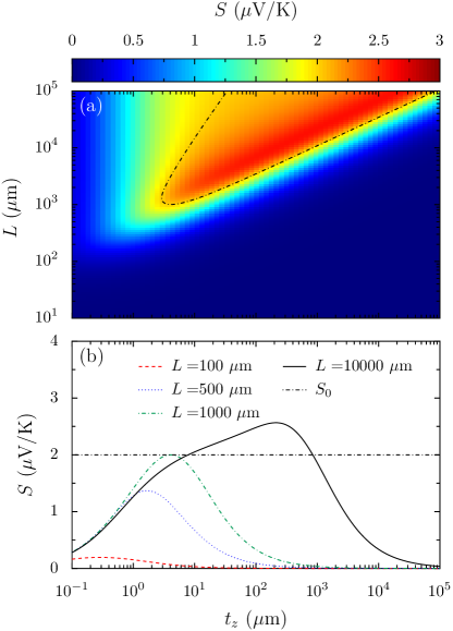
Figure 3: Induced thermopower between two gold films separated by a gap distance $d=6\;$Å as a function of the film thickness $t_{z}$, held at $T_{0}=300\;$K and $\Delta T=100\;$K, and a resistance of $R=22\;$m$\Omega$. In (a) the Seebeck coefficient is represented in a density plot as function of $L$ and $t_{z}$. Dash-dotted line indicates the value of $S_{0}$. In (b) we represent two dimensional cuts of (a) for different $L$. The dash-dotted line indicates the Seebeck coefficient $S_{0}$ of gold (bulk).

Let us now investigate the inverse induced thermoelectric effect. In this case we consider the configuration as depicted in Fig. 1(b). A bias voltage is applied along body 1 [$\phi_{1}(0)=0$ and $\phi_{1}(L)=\Delta\phi_{1}$] and its two ends are coupled to a thermostat at the same temperature [$T_{1}(0)=T_{1}(L)=T_{0}$]. As the second body is concerned, it is also coupled to the same thermostat on its left side [$T_{2}(0)=T_{0}$] and thermally insulated on its opposite side [$\Phi_{2}(L)=0$] for simplicity. Moreover, this film is an open circuit so that no electric current can flow through it [$J_{2}(0)=J_{2}(L)=0$]. We show that a current in body 1 can induce a thermal current in body 2. The heating or cooling which can be induced in the second film when an electric current flow in the first one can be quantified by the induced Peltier coefficient $\Pi=\Phi_{2}(0)/J_{1}(0)$. We remind that for a single body at temperature $T_{0}$, this coefficient satisfies $\Pi_{0}=S_{0}\>T_{0}$. In Fig. 4(a) we show the evolution of $\Pi$ with respect to the gap thickness and intensity of electric current flowing through body 1.

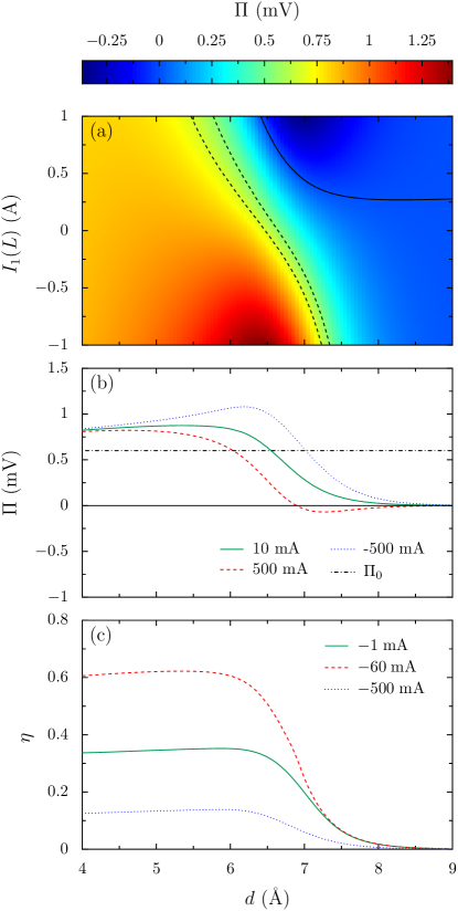
Figure 4: Induced Peltier coefficient and cooling efficiency as a function of $d$ for two gold films of $t_{z}=1\;\mu$m, $L=1000\;\mu$m and $T_{0}=300\;$K. (a) Induced Peltier coefficients as a function of the current in body 1 and $d$. Dashed lines correspond to $\Pi_{0}=S_{0}T_{0}$ of gold $\pm 10\%$, and the solid line represents $\Pi=0$. Cuts of (a) are shown in panel (b) for 10 mA (solid line), 500 mA (dashed line) and -500 mA (dotted line). The black dotted line represents $\Pi_{0}$. (c) Cooling efficiency as a function of $d$ for $-1\;$mA (solid line), $-500\;$mA (dotted line) and $-60\;$mA (dashed line).

When the current is negative, i.e. goes from right to left, $\Pi$ remains positive and asymptotically vanishes for large $d$. As for the induced Seebeck effect, the induced Peltier effect can exceed the bulk value $\Pi_{0}$ at short range distances thanks to electron tunneling. This induced effect can also change sign. Hence $\Pi$ can become negative for distances smaller than 1 nm and the electric current $I_{1}(L)$ is positive (from left to right). In this case the Peltier effect heats up the second solid. Moreover we see in Fig. 4(b) that above 8 Å the induced Peltier coefficient rapidly decreases whatever the electric current flowing through body 1. However, below this threshold, the it has a strong dependence on the current and can go beyond $2\Pi_{0}$ for $d=6.5\>A$ when a current $I_{1}=-500\;$mA is flowing in body 1. This corresponds to an extracted power through the left side of body 2 of $50\>$W/cm² . This flux is larger than most of thermoelectric cooling devices.

To conclude we analyze the cooling efficiency of induced Peltier effect, defined as

$$\eta=-\frac{\Phi^{-}_{2}(0)}{\Phi_{1}^{+}(0)-\Phi^{-}_{1}(L)-I_{1}(L)\Delta\phi_{1}},$$ (10)

where $-I_{1}(L)\Delta\phi_{1}\geq 0$ is the electrical power injected by the battery, and $\Phi^{+}_{i}(x)=\operatorname{max}\{\Phi_{i}(x),0\}$ and $\Phi^{-}_{i}(x)=\operatorname{min}\{\Phi_{i}(x),0\}$ are to be accounted when there is heat entering the system through the thermal reservoirs. In Fig. 4(c) we represent this efficiency for different values of current applied in film 1. We see that $\eta$ reaches a maximum at a given value of the current [about $I_{1}(0)=-60\;$mA], and it decreases for smaller and larger values. The cooling efficiency can reach values of about 60%, an efficiency comparable and even greater than that of current thermoelectric cooling systems Riffat and of conventional Rankine systems based on compression/expansion cycles Kaushikt .

In summary, we have highlighted two thermoelectric effects induced by electron tunneling between two closely separated conducting films. We have demonstrated that the induced Seebeck and Peltier effects can exceed the classical thermoelectric properties of bulk material when the films are separated by subnanometric gaps. We have shown that the induced Seebeck effect is very sensitive to the separation distance, making the measurement of the induced thermopower a promising method to quantify the extreme-near-field transfer between two conductors. Beside this effect we have highlighted the conditions to extract thermal power from a solid using the Peltier effect induced by electron tunneling and shown that the performances of this effect are comparable and even better than the classical compression-cycle systems. These thermoelectric effects could be exploited for nanoscale energy conversion and to develop solid-state refrigeration devices.

References

(1) A. Majumdar, Science 303, 777 (2004).
(2) P. Rodgers, Nature Nanotech. 3,76 (2008).
(3) S. R. de Groot and P. Mazur, Non-equilibrium thermodynamics (Dover, New York, 1984).
(4) N. Pottier, Physique statistique hors d’équilibre, EDP Sciences, Paris (2006).
(5) S. Kou, and H. Akai. Solid State Comms. 276, 2 (2018).
(6) J. G. Simmons, J. Appl. Phys., 34, 6, 1793 (1963).
(7) M. V. Berry and K. E. Mount, Rep. Prog. Phys. 35, 315 (1972).
(8) M. Gómez Viloria, P. Ben-Abdallah and R. Messina, Phys. Rev. B 108, 195420 (2023)
(9) M. Gómez Viloria, Y. Guo, S. Merabia, P. Ben-Abdallah and R. Messina, Phys. Rev. B 107, 125414 (2023) .
(10) J. B. Xu, K. Läuger, R. Möller, K. Dransfeld, and I. H. Wilson, Appl. Phys. A 59, 155 (1994).
(11) D. Polder and M. Van Hove, Phys. Rev. B 4, 3303 (1971).
(12) U. M. Ascher, R. M. M. Mattheij, and R. D. Russell, Numerical Solution of Boundary Value Problems for Ordinary Differential Equations (Society for Industrial and Applied Mathematics, Philadelphia, 1987).
(13) N. Cusack and P. Kendall, Proc. Phys. Soc. 72, 898 (1958).
(14) S. B. Riffat and X. Ma, Int. J. Energy Res. 28, 753 (2004).
(15) S. C. Kaushik, A. Dubey, and M. Singh, Energy Convers. Mgmt. 35, 871 (1994).