User-Assisted Networked Sensing in OFDM Cellular Network with Erroneous Anchor Position Information

Abstract

In the sixth-generation (6G) integrated sensing and communication (ISAC) cellular network, base stations (BSs) can collaborate with each other to reap not only the cooperative communication gain, but also the networked sensing gain. In contrast to cooperative communication where both line-of-sight (LOS) paths and non-line-of-sight (NLOS) paths are useful, networked sensing mainly relies on the LOS paths. However, in practice, the number of BSs possessing LOS paths to a target can be small, leading to marginal networked sensing gain. Because the density of user equipments (UEs) is much larger than that of the BSs, this paper considers a UE-assisted networked sensing architecture, where a BS transmits communication signals in the downlink, while the UEs that receive the echo signals scattered by a target can cooperate with the BS to localize it. Under this scheme, however, the positions of the UEs are estimated by Global Positioning System (GPS) and subject to unknown errors. If some UEs with significantly erroneous position information are used as anchors, the localization performance can be severely degraded. Based on the outlier detection technique, this paper proposes an efficient method to select a subset of UEs with accurate position information as anchors for localizing the target. Numerical results show that our scheme can select good UEs as anchors with very high probability, indicating that networked sensing can be realized in practice with the aid of UEs.

Index Terms—  Integrated sensing and communication (ISAC), networked sensing, anchor position errors, localization.

1 Introduction

Thanks to the sufficient bandwidth at the millimeter wave (mmWave) band and the terahertz (THz) band as well as the large aperture array brought by the massive multiple-input multiple-output (MIMO) technique, the sixth-generation (6G) cellular network will be able to provide high-resolution sensing services [1, 2, 3, 4, 5]. One notable advantage of 6G-enabled sensing over radar sensing lies in the potential for large-scale networked sensing [6, 7]. Specifically, the widely deployed base stations (BSs) in the cellular network are inter-connected by the fronthaul/backhaul networks and can share their local information for better sensing performance. This philosophy is similar to that behind the cooperative communication techniques such as networked MIMO, cloud radio access network, etc.

However, there is a hurdle to implement networked sensing in 6G cellular network. For wireless communication, both line-of-sight (LOS) and non-line-of-sight (NLOS) channels are useful for conveying the information. Therefore, it is easy to find multiple BSs that can cooperatively transmit/receive messages to/from each user. For sensing, on the contrary, only the LOS paths are useful in many applications such as localization. In 6G network, it is quite possible that one target just has a LOS path to one BS. How to harvest the theoretical networked sensing gain in practical 6G network thus becomes a challenge.

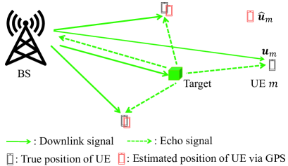
Fig. 1: System model of UE-assisted networked sensing.

To overcome this issue, this paper considers the utilization of user equipments (UEs) as additional anchors for networked sensing, because the density of the UEs is much larger than that of the BSs, and it is very likely to find UEs with LOS paths to a target. Specifically, our interested system aims to localize one target which merely has LOS paths to one BS and several UEs, as shown in Fig. 1. In such a system, the BS transmits the orthogonal frequency division multiplexing (OFDM) communication signals in the downlink, and the echo signals scattered by the target can be received by the BS and the UEs. Then, the BS and the UEs can respectively estimate their distances to the target and utilize the multilateration method to localize the target.

However, the positions of the UEs are estimated by Global Positioning System (GPS) and subject to unknown errors. Therefore, if all the UEs are utilized as the anchors to localize the target, the UEs with significantly erroneous position information can result in quite inaccurate localization results. Via employing the outlier detection technique [8, 9], this paper proposes an iterative method to select a subset of the UEs with small position errors for localizing the target. Specifically, in each iteration of our algorithm, if the removal of one UE can lead to a sufficiently large reduction in the residual for localizing the target, this UE will be deleted from the anchor set. Numerical results show that our proposed scheme can efficiently select the correct anchors for achieving accurate localization.

It is worth noting that the multilateration-based localization method with anchor position uncertainties has been investigated before in the literature [10, 11, 12, 13, 14]. In these works, the exact covariance matrices of the position errors are assumed to be known. Then, these information is used in defining the maximum likelihood (ML) problem to localize a target, such that the residuals associated with the anchors with smaller position errors are assigned with larger weights. As a result, the anchors with little position uncertainties can play a more significant role in localizing the target. However, in practice, it is difficult to obtain the covariance matrices of the errors in UE positions estimated by GPS. Under our proposed scheme, the outlier detection technique [8, 9] is utilized to remove the UEs with quite erroneous position information, even if no prior statistical information about the UE position errors is known.

2 System Model

We consider a 6G network based sensing system consisting of one BS, $M$ UEs, denoted by $\mathcal{M}=\{1,\dots,M\}$, and one target, where the BS and the UEs serve as the anchors to localize the target. Let $\boldsymbol{b}\in\mathbb{R}^{2\times 1}$, $\boldsymbol{u}_{m}\in\mathbb{R}^{2\times 1}$ , and $\boldsymbol{a}\in\mathbb{R}^{2\times 1}$ denote the locations of the BS, the $m$-th UE, $\forall m\in\mathcal{M}$, and the target, respectively. Then, we can define $d^{\rm BT}=\|\boldsymbol{b}-\boldsymbol{a}\|$ and $d^{\rm UT}_{m}=\|\boldsymbol{u}_{m}-\boldsymbol{a}\|$ as the true distance between the BS and the target and that between UE $m$ and the target, respectively, $\forall m$. Moreover, the sum of the distance between the BS and the target and that between UE $m$ and the target is $d^{\rm BTU}_{m}=d^{\rm BT}+d^{\rm UT}_{m},\forall m.$ However, in practice, the BS’s location is fixed and perfectly known, while the UEs’ locations are typically estimated via the GPS and subject to estimation errors. Define $\hat{\boldsymbol{u}}_{m}=\boldsymbol{u}_{m}+\Delta\boldsymbol{u}_{m}$ as the estimated position of UE $m$ made by GPS, where $\Delta\boldsymbol{u}_{m}$ denotes the unknown position estimation error, $\forall m$. Because the location of UE $m$ is known as $\hat{\boldsymbol{u}}_{m}$, instead of $\boldsymbol{u}_{m}$, given any target location $\boldsymbol{a}$, the estimated values of $d_{m}^{\rm UT}$ and $d_{m}^{\rm BTU}$ are $\|\hat{\boldsymbol{u}}_{m}-\boldsymbol{a}\|$ and $\|\boldsymbol{b}-\boldsymbol{a}\|+\|\hat{\boldsymbol{u}}_{m}-\boldsymbol{a}\|$, respectively, $\forall m$.

In our considered system, the BS transmits OFDM-based downlink communication signals such that the BS and the UEs can localize the target according to their received echoes scattered by the target. Let $\boldsymbol{s}=[s_{1},\dots,s_{N}]$ denote the frequency-domain OFDM symbol sent from the BS, where $N$ denotes the number of sub-carriers and $s_{n}$ denotes the unit-power transmitted sample at the $n$-th sub-carrier, $\forall n$. Then, the corresponding time-domain OFDM signal of the BS is $\boldsymbol{\chi}=\left[\chi_{1},\dots,\chi_{N}\right]^{T}=\boldsymbol{W}^{H}\sqrt{p}\boldsymbol{s},$ where $\chi_{n}$ denotes the $n$-th sample transmitted by the BS, $p$ denotes the transmission power at the BS, and $\boldsymbol{W}\in\mathbb{C}^{N\times N}$ denotes the discrete Fourier transform (DFT) matrix. Note that the duration of each OFDM sample period is $1/N\Delta f$ seconds (s), where $\Delta f$ in Hz denotes the OFDM sub-carrier spacing. After inserting the cyclic prefix (CP) consisting of $Q$ OFDM samples, the time-domain signal transmitted by the BS over one OFDM symbol period is given by $\bar{{\boldsymbol{\chi}}}=[\bar{\chi}_{-Q},\dots,\bar{\chi}_{-1},\bar{\chi}_{0},\dots,\bar{\chi}_{N-1}]$, where $\bar{\chi}_{n}=\chi_{N+n+1}$ denotes the CP when $n\leq 0$, and $\bar{\chi}_{n}=\chi_{n+1}$ denotes the useful signal when $n>0$. Define $\boldsymbol{h}^{\rm BTB}=[h_{0}^{\rm BTB},\dots,h_{L-1}^{\rm BTB}]$ as the $L$-tap baseband equivalent channel from the BS via the target to the BS, where $L$ denotes the maximum number of detectable paths. Because we only consider one target in our system, there should be only one $l^{\ast}\leq L$ satisfying $h_{l^{\ast}}^{\rm BTB}\neq 0$, where $l^{\ast}$ denotes the propagation delay (in terms of OFDM sample periods) from the BS to the target and back to the BS. Then, the received signal at the BS in the $n$-th OFDM sample period is expressed as

$$y_{n}=\sum_{l=0}^{L-1}h_{l}^{\rm BTB}\bar{\chi}_{n-l}+z_{n},\forall n,\vspace{-0.2cm}$$ (1)

where $z_{n}\sim\mathcal{CN}(0,\sigma^{2})$ denotes the noise at the BS in the $n$-th OFDM sample period, with $\sigma^{2}$ denoting the average noise power.

Each UE can also receive the signals via two links: the direct link from the BS to the UE and the cascaded link from the BS to the target to the UE. In practice, the UEs are not perfectly synchronized in time with the BS. Define the sampling timing offset (STO) between the BS and UE $m$ as $\tau_{m}$ OFDM sample periods, $\forall m$, i.e., if the local clock time at UE $m$ is $t_{m}$, then that at the BS is $t=t_{m}+\tau_{m}$. Specifically, we have $\tau_{m}>0$ if the clock time at UE $m$ is earlier, while $\tau_{m}<0$ otherwise. Let $\boldsymbol{h}_{m}^{\rm BU}=[h_{m,0}^{\rm BU},\dots,h_{m,L-1}^{\rm BU}]$ denote the $L$-tap multipath channel from the BS to UE $m$. Note that $h_{m,l^{\ast}}^{\rm BU}\neq 0$ holds if and only if $l^{\ast}$ is the delay (in terms of OFDM sample periods) of the propagation either from the BS to UE $m$ or from the BS to the target to UE $m$. Then, the received time-domain OFDM signal at UE $m$ in the $n$-th OFDM sample period is given by

$$y_{m,n}=\sum_{l=0}^{L-1}h_{m,l}^{\rm BU}\bar{\chi}_{n-l-\tau_{m}}+z_{m,n},\forall m,n,\vspace{-0.1cm}$$ (2)

where $z_{m,n}\sim\mathcal{CN}(0,\sigma_{m}^{2})$ denotes the noise at UE $m$ in the $n$-th OFDM sample period, with $\sigma_{m}^{2}$ denoting the average noise power.

In this paper, we adopt a two-phase networked sensing protocol for target localization. Specifically, in Phase I, the BS and each UE first estimate the time-domain channels based on (1) and (2), and then estimate $d^{\rm BT}$ and $d_{m}^{\rm BTU}$’s based on the non-zero entries of the estimated channels. Let $\bar{d}^{\rm BT}$ and $\bar{d}_{m}^{\rm BTU}$’s denote the above estimations. Then, $\bar{d}^{\rm UT}_{m}=\bar{d}^{\rm BTU}_{m}-\bar{d}^{\rm BT}$ is the estimated distance between the target and UE $m,\forall m$. The main difficulty that we need to tackle lies in the estimation of $d_{m}^{\rm BTU}$’s since the BS and the UEs are not perfectly synchronized and the estimated propagation delays from the BS to the target to the UEs will be shifted by the unknown STOs $\tau_{m}$’s. Then, in Phase II, given the range information obtained in Phase I, we will estimate the target location using the multilateration method based on the following relationship to the anchors

$$\|\boldsymbol{b}-\boldsymbol{a}\|=\bar{d}^{\rm BT}+\eta,\vspace{-0.1cm}$$ (3)

$$\|\hat{\boldsymbol{u}}_{m}-\boldsymbol{a}\|=\bar{d}^{\rm UT}_{m}+\gamma_{m},\forall m,\vspace{-0.1cm}$$ (4)

where $\eta$ and $\gamma_{m}$ denote the corresponding estimation errors. Note that under the traditional multilateration method, the locations of the anchors are assumed to be perfectly known. However, a new challenge for localization arises in our interested system—the locations of the UEs (anchors) are estimated by the GPS and subject to unknown (and maybe significant) errors $\Delta\boldsymbol{u}_{m}$’s. In other words, if we simply use all the UEs as anchors, it is quite possible that $\gamma_{m}$’s are very large for some $m$’s and the corresponding estimated location of the target is very inaccurate. In Phase II, our main job is to select the best subset of the UEs as anchors to perform the multilateration method with high localization accuracy. In the following, we provide detailed information about Phase I and Phase II under the above protocol.

3 Phase I: Range Estimation

In this section, we introduce the proposed range estimation method based on the received signals in Phase I of the two-phase sensing protocol. It can be shown that the signal received by the BS in the frequency domain is given by [7]

$$\bar{\boldsymbol{y}}=\sqrt{p}\operatorname{diag}{(\boldsymbol{s})}\boldsymbol{G}\boldsymbol{h}^{\rm BTB}+\bar{\boldsymbol{z}},\vspace{-0.2cm}$$ (5)

where $\operatorname{diag}{(\boldsymbol{s})}$ is a diagonal matrix with the main diagonal being $\boldsymbol{s}$, $\boldsymbol{G}\in\mathbb{C}^{N\times L}$ with the $(n,l)$-th element being $G_{n,l}=e^{\frac{-j2\pi(n-1)(l-1)}{N}}$, and $\bar{\boldsymbol{z}}=\boldsymbol{W}^{H}[z_{1},\dots,z_{N}]^{T}\sim\mathcal{CN}(0,\sigma^{2}\boldsymbol{I})$. Since there is only one target in the system, $\boldsymbol{h}^{\rm BTB}$ is a sparse vector with one non-zero element. Thus, the LASSO technique can be utilized to estimate the time-domain channel $\boldsymbol{h}^{\rm BTB}$ by solving the following problem

$$\!\!\!\!\!\mbox{}\!\!\underset{\scriptstyle\boldsymbol{h}^{\rm BTB}}{\min}\!\! \quad\frac{1}{2}\|\bar{\boldsymbol{y}}-\sqrt{p}\operatorname{diag}(\boldsymbol{s})\boldsymbol{G}\boldsymbol{h}^{\rm BTB}\|_{2}^{2}+\lambda\|\boldsymbol{h}^{\rm BTB}\|_{1},\vspace{-0.3cm}$$ (6)

where $\lambda>0$ is a given coefficient to make sure that in the optimal solution to problem (6), there is only one non-zero element. Problem (6) is convex and can be efficiently solved by using existing solvers, e.g., CVX. Let $\bar{\boldsymbol{h}}^{\rm BTB}=\left[\bar{h}_{1}^{\rm BTB},\dots,\bar{h}_{L}^{\rm BTB}\right]^{T}$ denote the optimal solution of problem (6), and $l^{\ast}$ denote the index of the sole non-zero element in $\bar{\boldsymbol{h}}^{\rm BTB}$, i.e., $\bar{h}_{l^{\ast}}^{\rm BTB}\neq 0$. Then, the range between the BS and the target, i.e., $d^{\rm BT}$, is estimated as follows [7]

$$\bar{d}^{\rm BT}=l^{\ast}c_{0}/(2N\Delta f)+c_{0}/(4N\Delta f),\vspace{-0.1cm}$$ (7)

where $c_{0}$ denotes the speed of light.

Next, we focus on estimating the range of the path from the BS to the target to UE $m$, i.e., $d_{m}^{\rm BTU}$, based on the received signal at UE $m$, $\forall m$. To this end, we first need to estimate $\boldsymbol{h}_{m}^{\rm BU}$’s. However, different from the case for processing the signals received by the BS as shown in the above, the unknown STOs, i.e., $\tau_{m}$’s, make it hard to estimate $h_{m,l}^{\rm BU}$’s based on the signals received by the UEs, i.e., (2). To tackle this challenge, we first define $l_{m}=\lfloor N\Delta f\|\boldsymbol{b}-\boldsymbol{u}_{m}\|/c_{0}\rfloor$ as the propagation delay (in terms of OFDM sample periods) of the LOS path from the BS to UE $m$, where $\lfloor\cdot\rfloor$ is the floor function. Then, we can reformulate (2) as

$$y_{m,n} \overset{(a)}{=}\sum_{l=l_{m}}^{L-1}h_{m,l}^{\rm BU}\bar{\chi}_{n-l-\tau_{m}}+z_{m,n}$$ (8)

$$=\sum_{l=l_{m}+\tau_{m}}^{L+\tau_{m}-1}h_{m,l-\tau_{m}}^{\rm BU}\bar{\chi}_{n-l}+z_{m,n}$$

$$=\sum_{l=0}^{L+\tau_{m}-1}\tilde{h}_{m,l}^{\rm BU}\bar{\chi}_{n-l}+z_{m,n},\forall m,n,$$

where $(a)$ holds as no path with a delay of $l<l_{m}$ OFDM sample periods exits between the BS and UE $m$, i.e., $h_{m,l}^{\rm BU}=0,l\in[0,l_{m})$ and $\tilde{h}_{m,l}^{\rm BU}$ is defined as

$$\tilde{h}_{m,l}^{\rm BU}=\begin{cases}&h_{m,l-\tau_{m}}^{\rm BU},\quad\text{if}~{}l\in[l_{m}+\tau_{m},L+\tau_{m}-1],\\ &0,\quad\quad~{}\text{otherwise}.\end{cases}\vspace{-0.2cm}$$ (9)

Therefore, $\tilde{h}_{m,l}^{\rm BU}$ can be interpreted as the virtual channel associated with a path between the BS and UE $m$, where the imperfectly synchronized UE $m$ believes the path delay to be $l$ OFDM sample period, but it is actually $l-\tau_{m}$ OFDM sample periods. In this paper, we assume that $l_{m}+\tau_{m}\geq 0$, such that UE $m$ sees no inter-symbol interference (ISI) from the next OFDM symbol sent by the BS even when the BS’s clock is earlier than that at UE $m$, i.e., $\tau_{m}<0$, $\forall m$.

Note that there is no STO, i.e., $\tau_{m}$, in the reformulated signal model (8), implying that $\tilde{h}_{m,l}^{\rm BU}$’s can be estimated by applying the conventional OFDM channel estimation techniques. However, the propagation delays estimated based on $\tilde{h}_{m,l}^{\rm BU}$ will be shifted by the unknown STO—$\tilde{h}_{m,l}^{\rm BU}\neq 0$ indicates that there is a path from the BS to UE $m$ whose propagation delay is of $l-\tau_{m}$, instead of $l$, OFDM sample periods. Thus, we can never obtain correct delay/range estimations without knowing the STOs. In the following, we propose an efficient method that can first estimate the STOs based on the LOS signals from the BS to the UEs, and then utilize the STOs to estimate the propagation delays from the BS to the target to the UEs.

Specifically, according to (8), the received signal at UE $m$ in the frequency domain is given by

$$\bar{\boldsymbol{y}}_{m}=\sqrt{p}\operatorname{diag}{(\boldsymbol{s})}\boldsymbol{G}_{m}\tilde{\boldsymbol{h}}^{\rm BU}_{m}+\bar{\boldsymbol{z}}_{m},\forall m,\vspace{-0.2cm}$$ (10)

where $\boldsymbol{G}_{m}\in\mathbb{C}^{N\times(L+\tau_{m})}$ with the $(n,l)$-th element being $G_{m,n,l}=e^{\frac{-j2\pi(n-1)(l-1)}{N}}$, $\tilde{\boldsymbol{h}}^{\rm BU}_{m}=[\tilde{h}_{m,0}^{\rm BU},\dots,\tilde{h}_{m,L+\tau_{m}-1}^{\rm BU}]$, and $\bar{\boldsymbol{z}}_{m}=\boldsymbol{W}^{H}[z_{m,1},\dots,z_{m,N}]^{T}\sim\mathcal{CN}(0,\sigma_{m}^{2}\boldsymbol{I})$.

In this paper, we assume that all the UEs know the signal $\boldsymbol{s}$ sent by the BS (e.g., $\boldsymbol{s}$ can be the known pilot signal). Moreover, $\tilde{\boldsymbol{h}}_{m}^{\rm BU}$ is a sparse channel vector with only two elements being non-zero. Thus, the virtual channel between the BS and UE $m$ as defined in (9) can be estimated by solving the following convex optimization problem

$$\!\!\!\!\!\mbox{}\!\!\underset{\scriptstyle\tilde{\boldsymbol{h}}_{m}^{\rm BU}}{\min}\!\! \quad\frac{1}{2}\|\bar{\boldsymbol{y}}_{m}-\sqrt{p}\operatorname{diag}(\boldsymbol{s})\boldsymbol{G}_{m}\tilde{\boldsymbol{h}}^{\rm BU}_{m}\|_{2}^{2}+\lambda\|\tilde{\boldsymbol{h}}^{\rm BU}_{m}\|_{1}.\vspace{-0.3cm}$$ (11)

Let $\bar{\boldsymbol{h}}_{m}^{\rm BU}=[\bar{h}_{m,0}^{\rm BU},\dots,\bar{h}_{m,L_{m}-1}^{\rm BU}]^{T}$ denote the optimal solution to problem (11). If $\bar{h}_{m,l^{\ast}}^{\rm BU}\neq 0$ for some $l^{\ast}$, then there is a path between the BS and UE $m$, whose propagation delay is of $l^{\ast}-\tau_{m}$ OFDM sample periods. Thus, we can define

$$\bar{l}_{m}=\min\{l|\forall l~{}\text{with}~{}\bar{h}^{\rm BU}_{m,l}\neq 0\}\vspace{-0.2cm}$$ (12)

as the estimated propagation delay of the direct path between the BS and UE $m$, when their clocks differ by $\tau_{m}$ OFDM sample periods, $\forall m$. Note that the position of the BS and the estimated position of UE $m$ imply that the propagation delay between them should be

$$\tilde{l}_{m}=\lfloor N\Delta f\|\boldsymbol{b}-\hat{\boldsymbol{u}}_{m}\|/c_{0}\rfloor,\forall m.\vspace{-0.2cm}$$ (13)

Then, the STO between the BS and UE $m$ is estimated as

$$\hat{\tau}_{m}=\bar{l}_{m}-\tilde{l}_{m},\forall m.\vspace{-0.2cm}$$ (14)

Next, let us denote the index of another non-zero element in $\bar{h}_{m}^{\rm BU}$ as $l^{\ast}$ ($l^{\ast}\neq\bar{l}_{m}$). Then, the range of the path from the BS to the target to UE $m$ is estimated as

$$\bar{d}_{m}^{\rm BTU}=(l^{\ast}-\hat{\tau}_{m})c_{0}/(N\Delta f)+c_{0}/(2N\Delta f),\forall m.\vspace{-0.1cm}$$ (15)

Last, the range from the target to UE $m$ is estimated as follows

$$\bar{d}^{\rm UT}_{m}=\bar{d}^{\rm BTU}_{m}-\bar{d}^{\rm BT},\forall m,\vspace{-0.1cm}$$ (16)

where $\bar{d}^{\rm BT}$ is given in (7).

In summary, following Phase I, the estimated ranges from the target to all the anchors, i.e., $\bar{d}^{\rm BT}$ and $\bar{d}^{\rm UT}_{m},\forall m$, can be obtained. Then, these information together with the UEs’ position information will be sent to the cloud for localization.

4 Phase II: Target localization via removing ineffective anchors

In Phase II, we aim to localize the target based on the multilateration method [15]. To successfully localize the target, it requires both accurate information about the anchor positions and the ranges from the target to the anchors. However, in practice, the positions of some UEs estimated via the GPS may be highly inaccurate. Moreover, if $\hat{\boldsymbol{u}}_{m}$ is quite inaccurate compared to $\boldsymbol{u}_{m}$, then $\tilde{l}_{m}$ given in (13) is a poor estimation of the propagation delay for the LOS path between the BS and UE $m$, leading to wrong estimation of the STO $\tau_{m}$ given in (14) as well as that of $d^{\rm BTU}_{m}$ given in (15). Therefore, the UEs whose positions estimated by the GPS are quite inaccurate may significantly degrade the performance of target localization and should not be used as anchors.

In this section, we adopt the outlier detection technique [8, 9] to remove the UEs with inaccurate position information such that the BS together with the effective UEs with accurate position information can jointly localize the target. Specifically, denote $\tilde{\mathcal{M}}$ with $|\tilde{\mathcal{M}}|\geq 2$ as a subset of $\mathcal{M}$, i.e., $\tilde{\mathcal{M}}\subseteq\mathcal{M}$. Then, if merely the BS and the UEs in $\tilde{\mathcal{M}}$ serve as anchors, the target can be localized based on the multilateration method by solving the following weighted nonlinear least squares problem [16]

$$\!\!\!\!\!\mbox{}\!\!\underset{\scriptstyle\boldsymbol{a}}{\min}\!\! \quad v\left(\|\boldsymbol{b}-\boldsymbol{a}\|-\bar{d}^{\rm BT}\right)^{2}+\sum_{m\in\tilde{\mathcal{M}}}\left(\|\hat{\boldsymbol{u}}_{m}-\boldsymbol{a}\|-\bar{d}_{m}^{\rm UT}\right)^{2},\vspace{-0.2cm}$$ (17)

where $\left(\|\boldsymbol{b}-\boldsymbol{a}\|-\bar{d}^{\rm BT}\right)^{2}$ and $\left(\|\hat{\boldsymbol{u}}_{m}-\boldsymbol{a}\|-\bar{d}_{m}^{\rm UT}\right)^{2}$ are the residuals associated with the BS and UE $m$, respectively, $\forall m$, and $v$ is the weight of the residual corresponding to the BS. Note that the residual associated with the BS is much more trustworthy than that associated with a UE, because the estimated positions of the UEs are subject to errors. Thus, we set $v>1$, such that the residual associated with the BS plays a more significant role in determining the location of the target.

Problem (17) can be efficiently solved via the Gauss-Newton method [15]. Let us define $\theta(\tilde{\mathcal{M}})$ as the objective value of problem (17) achieved by the Gauss-Newton method given the UE set $\tilde{\mathcal{M}}$. Moreover, to reduce the dependence on the number of anchors for localization, we define

$$\bar{\theta}(\tilde{\mathcal{M}})=\theta(\tilde{\mathcal{M}})/(|\tilde{\mathcal{M}}|+1)\vspace{-0.1cm}$$ (18)

as the normalized residual for using the BS and the UEs in $\tilde{\mathcal{M}}$ as anchors to localize the target [17]. Our goal in this paper is to select the UEs for localizing the target by solving the following problem

$$\!\!\!\!\!\mbox{}\!\!\underset{\scriptstyle\tilde{\mathcal{M}}\subseteq\mathcal{M}}{\min} \quad\bar{\theta}(\tilde{\mathcal{M}}).$$ (19)

One straightforward way to solve the above problem is via exhaustive search. However, this method is of prohibitively high complexity. To this end, we propose an iterative algorithm with low complexity to solve problem (19). Note that if the positions of the anchors estimated by the GPS are all correct, then the performance for localizing the target will improve with the number of anchors [18]. This motivates us to find as many effective UEs with accurate position information as possible to localize the target. Inspired by this observation, our proposed iterative algorithm starts with the original set $\mathcal{M}$, and removes one ineffective UE with inaccurate position estimated by the GPS in each iteration, until no significant gain is obtained by removing an UE. Specifically, define $\tilde{\mathcal{M}}_{k}$ as the set of UEs that are not removed from $\mathcal{M}$ after the $k$-th iteration with $|\tilde{\mathcal{M}}_{k}|=M-k$, $\forall k$. Note that in the initialization step, we set $\tilde{\mathcal{M}}_{0}=\mathcal{M}$. The way to remove one UE from set $\tilde{\mathcal{M}}_{k-1}$ in the $k$-th iteration of our proposed algorithm is as follows. Define

$$\mathcal{Q}_{k}=\{\mathcal{M}_{k}|\mathcal{M}_{k}\subseteq\tilde{\mathcal{M}}_{k-1},|\mathcal{M}_{k}|=|\tilde{\mathcal{M}}_{k-1}|-1\}$$ (20)

as the set of all possible solutions in the $k$-th iteration of the algorithm. According to problem (19), at the $k$-th iteration of our algorithm, we set $\tilde{\mathcal{M}}_{k}$ as the optimal solution to the following problem

$$\!\!\!\!\!\mbox{}\!\!\underset{\scriptstyle\tilde{\mathcal{M}}_{k}\in\mathcal{Q}_{k}}{\min} \quad\bar{\theta}(\tilde{\mathcal{M}}_{k}).$$ (21)

Note that problem (21) can be solved via the exhaustive research method efficiently because $|\mathcal{Q}_{k}|=M-k+1,\forall k$. Therefore, in the $k$-th iteration of the algorithm, if the removal of a UE from the anchor set $\tilde{\mathcal{M}}_{k-1}$ can lead to the minimum normalized residual for localizing the target, we just remove this UE. If after the $k^{\ast}$-th iteration, $\bar{\theta}(\tilde{\mathcal{M}}_{k^{\ast}-1})-\bar{\theta}(\tilde{\mathcal{M}}_{k^{\ast}})\leq\theta_{\rm th}$, where $\theta_{\rm th}$ is a given threshold, then it indicates that removing an UE from the anchor set can no longer significantly reduce the localization residual. Then, we will terminate our algorithm and set $\tilde{\mathcal{M}}_{k^{\ast}-1}$ as the solution to problem (19). Last, the corresponding solution of (17) with $\tilde{\mathcal{M}}=\tilde{\mathcal{M}}_{k^{\ast}-1}$ is the final estimation of the target location.

The above algorithm is of low complexity. Specifically, with the exhaustive search method for problem (19), we need to solve problem (17) for $D_{1}=\sum_{n=2}^{M}\tbinom{M}{n}=\sum_{n=2}^{M}\frac{M!}{n!(M-n)!}$ times. However, under our proposed algorithm, in the $k$-th iteration ($k\geq 1$), we only need to solve problem (17) for $M-k+1$ times. The algorithm reaches its worst-case complexity when it stops at $k=M-2$ (when only two UEs and the BS serve as three anchors). In this case, we need to solve problem (17) for $D_{2}=\sum_{k=1}^{M-2}M-k+1=\frac{(M-2)(M+3)}{2}$ times.

5 Numerical Results

In this section, we provide numerical results to verify the effectiveness of the proposed two-phase target localization protocol. The channel bandwidth is assumed to be $B=N\Delta f$ = 400 MHz. Moreover, the BS, the UEs, and the target are uniformly distributed in a 100 m $\times$ 100 m square. The position uncertainty of UE $m$, i.e., $\Delta\boldsymbol{u}_{m}$, is modeled as a zero-mean Gaussian random vector with covariance matrix $\boldsymbol{\Phi}_{m},\forall m$ [13]. In the simulations, we set $\boldsymbol{\Phi}_{m}=-20\boldsymbol{I}_{2}~{}\text{dBm}^{2}$ for the effective UEs, while for the other UEs, we set $\boldsymbol{\Phi}_{m}=20\boldsymbol{I}_{2}~{}\text{dBm}^{2}$, with $\boldsymbol{I}_{2}$ being the identity matrix of size 2. Furthermore, in problem (17), we set $v=10$.

Fig. 2: Localization error probability versus the number of ineffective UEs when 4 effective UEs exist.

Fig. 2 shows the localization error probability of our proposed algorithm when the number of effective UEs with accurate position information is fixed as 4, and that of ineffective UEs with inaccurate position information ranges from 1 to 5. Here, an error event for localizing the target is defined as the case that the estimated location does not lie within a radius of 1 m from the true target location. Moreover, we adopt the scheme that selects all the UEs, no matter their position information estimated by the GPS is correct or not, as anchors to localize the target as the benchmark scheme. It is observed that by carefully selecting the UEs as the anchors, our proposed scheme can indeed significantly improve the localization performance over the benchmark scheme. Finally, numerical results also verify that our proposed algorithm is low-complexity. For example, when there are 1 BS, 4 effective UEs, and 3 ineffective UEs, i.e., $M=7$, the average CPU running time to localize the target is about 0.6 s.

6 Conclusion

In this paper, we considered a UE-assisted networked sensing architecture in 6G network, where one BS and multiple UEs serve as anchors to localize one target. A two-phase protocol was designed, where the ranges from the target to the BS as well as to the UEs are estimated in Phase I, and the multilateration method is applied to localize the target in Phase II. One challenge of this scheme is that the estimated positions of some UEs via GPS may suffer from large errors, leading to poor localization performance under the multilateration method. To tackle this issue, under Phase II of our proposed protocol, we proposed an efficient method to remove the UEs with quite inaccurate position information from the anchor set such that the remaining anchors can localize the target with high performance. Numerical results were provided to verify the effectiveness of our proposed UE selection scheme for localization.

References

- [1] F. Liu et al., “Integrated sensing and communications: Toward dual-functional wireless networks for 6G and beyond,” IEEE J. Sel. Areas Commun., vol. 40, no. 6, pp. 1728–1767, 2022.
- [2] L. Zheng, M. Lops, Y. C. Eldar, and X. Wang, “Radar and communication coexistence: An overview: A review of recent methods,” IEEE Signal Process. Mag., vol. 36, no. 5, pp. 85–99, 2019.
- [3] J. A. Zhang et al., “An overview of signal processing techniques for joint communication and radar sensing,” IEEE J. Sel. Top. Signal Process., vol. 15, no. 6, pp. 1295–1315, 2021.
- [4] A. Hassanien, M. G. Amin, E. Aboutanios, and B. Himed, “Dual-function radar communication systems: A solution to the spectrum congestion problem,” IEEE Signal Process. Mag., vol. 36, no. 5, pp. 115–126, 2019.
- [5] A. Liu et al., “A survey on fundamental limits of integrated sensing and communication,” IEEE Commun. Surv. Tutorials, vol. 24, no. 2, pp. 994–1034, 2022.
- [6] H. Wymeersch, J. Lien, and M. Z. Win, “Cooperative localization in wireless networks,” Proc. IEEE, vol. 97, no. 2, pp. 427–450, 2009.
- [7] Q. Shi, L. Liu, S. Zhang, and S. Cui, “Device-free sensing in OFDM cellular network,” IEEE J. Sel. Areas Commun., vol. 40, no. 6, pp. 1838–1853, 2022.
- [8] X. Li, “An iterative NLOS mitigation algorithm for location estimation in sensor networks,” in Proc. 15th IST Mobile Wireless Commun. Summit, 2006, pp. 1–5.
- [9] I. Guvenc and C. C. Chong, “A survey on TOA based wireless localization and NLOS mitigation techniques,” IEEE Commun. Surv. Tutorials, vol. 11, no. 3, pp. 107–124, 2009.
- [10] Q. Shi, C. He, H. Chen, and L. Jiang, “Distributed wireless sensor network localization via sequential greedy optimization algorithm,” IEEE Trans. Signal Process., vol. 58, no. 6, pp. 3328–3340, 2010.
- [11] P. M. Ghari, R. Shahbazian, and S. A. Ghorashi, “Maximum entropy-based semi-definite programming for wireless sensor network localization,” IEEE Internet Things J., vol. 6, no. 2, pp. 3480–3491, 2019.
- [12] K. W. K. Lui, W.-K. Ma, H. C. So, and F. K. W. Chan, “Semi-definite programming algorithms for sensor network node localization with uncertainties in anchor positions and/or propagation speed,” IEEE Trans. Signal Process., vol. 57, no. 2, pp. 752–763, 2009.
- [13] G. Naddafzadeh-Shirazi, M. B. Shenouda, and L. Lampe, “Second order cone programming for sensor network localization with anchor position uncertainty,” IEEE Trans. Wireless Commun., vol. 13, no. 2, pp. 749–763, 2014.
- [14] M. Angjelichinoski, D. Denkovski, V. Atanasovski, and L. Gavrilovska, “Cramér–Rao lower bounds of RSS-based localization with anchor position uncertainty,” IEEE Trans. Inf. Theory, vol. 61, no. 5, pp. 2807–2834, 2015.
- [15] D. J. Torrieri, “Statistical theory of passive location systems,” IEEE Trans. Aerosp. Electron. Syst., vol. AES-20, no. 2, pp. 183–198, 1984.
- [16] J. J. Caffery and G. L. Stuber, “Overview of radiolocation in CDMA cellular systems,” IEEE Commun. Mag., vol. 36, no. 4, pp. 38–45, 1998.
- [17] P. C. Chen, “A non-line-of-sight error mitigation algorithm in location estimation,” in Proc. IEEE Int. Conf. Wireless Commun. Networking (WCNC), 1999, pp. 316–320.
- [18] R. Zekavat and R. M. Buehrer, Handbook of position location: Theory, practice and advances, vol. 27, John Wiley & Sons, 2011.