Multi-tracing the primordial Universe with future surveys

Abstract

The fluctuations generated by Inflation are Gaussian in the simplest models, but may be non-Gaussian in more complex models. Since these fluctuations seed the large-scale structure, any primordial non-Gaussianity of local type will leave an imprint on the tracer power spectrum on ultra-large scales. In order to combat the problem of growing cosmic variance on these scales, we use a multi-tracer analysis that combines different tracers of the matter distribution to maximise any primordial signal. In order to illustrate the advantages that can be brought by multi-tracing future surveys, we consider two pairs of (galaxy survey, 21cm intensity mapping survey), one at high redshift ($1\leq z\leq 2$) and one at very high redshift ($2\leq z\leq 5$). The 21cm surveys are in interferometer mode, and are idealised versions of HIRAX and PUMA. We implement foreground avoidance filters and use non-trivial models of the interferometer thermal noise. The galaxy surveys are idealised versions of Euclid and MegaMapper. Via a simple Fisher forecast we illustrate the potential of the multi-tracer. Our results show a $\sim 20-70\%$ improvement in precision on local primordial non-Gaussianity from the multi-tracer.

1 Introduction

Galaxy surveys in combination with cosmic microwave background (CMB) surveys have laid the foundations for precision cosmology. The next generation of surveys will deliver even higher precision by covering larger sky areas and deeper redshifts with better sensitivity. Each of these surveys is destined to make major advances in the precision and accuracy of the cosmological parameters of the standard LCDM model. At the same time, future surveys will look for signals beyond LCDM. One such signal arises if there is significant non-Gaussianity in the primordial perturbations that seed the CMB fluctuations and the large-scale structure.

Primordial non-Gaussianity (PNG) is a key probe of Inflation, which is currently the best framework that we have for the generation of seed fluctuations. The local type of PNG, described by the parameter $f_{\rm NL}$, if found to be nonzero, will rule out the simplest Inflation models [1]. Furthermore, if $0<|f_{\rm NL}|\lesssim 1$, then many other models can also be ruled out [2, 3]. In order to achieve this, a precision of $\sigma(f_{\rm NL})<1$ is required.

The best current 1$\sigma$ constraint comes from the Planck survey, via the CMB bispectrum [4]:

$$f_{\rm{NL}}=-0.9\pm 5.1\,.$$ (1.1)

The CMB power spectrum does not carry an imprint of local PNG, and the same is true for the matter power spectrum. However, the power spectrum of a biased tracer, such as galaxies, does contain a signal of local PNG on ultra-large scales – due to the phenomenon of scale-dependent bias [5, 6]. Constraints from future CMB surveys will not be able to reach $\sigma(f_{\rm NL})<1$ due to cosmic variance. In the case of galaxy surveys, the current best constraints are $\sigma(f_{\rm NL})\gtrsim 20$. Future galaxy surveys will improve on this, potentially reaching the CMB level of precision and beyond [7, 8]. Although galaxy power spectrum constraints on $f_{\rm NL}$ will be a powerful independent check on the CMB results, single-tracer constraints are unlikely to achieve $\sigma(f_{\rm NL})<1$, again because of cosmic variance, which is highest on precisely the scales where the local PNG signal is strongest.

Since the local PNG signature in large-scale structure depends on the particular tracer, it is possible to improve the precision on $f_{\rm NL}$ by combining the power spectra of different tracers. This multi-tracer approach can effectively remove cosmic variance [9, 10, 11, 12]. As a result, the multi-tracer of future galaxy surveys with intensity mapping of the 21cm emission of neutral hydrogen (HI IM surveys), can deliver significant improvements in the precision on $f_{\rm NL}$ (e.g. [13, 14, 15]) and in some cases it can in principle reach $\sigma(f_{\rm NL})<1$ (e.g. [16, 17, 18, 19, 20]). The multi-tracer can also mitigate some of the observational systematics in single-tracer surveys.

Here we follow [15] in considering pairs made of one spectroscopic galaxy survey and one HI intensity mapping survey. However, we consider HI IM surveys in interferometer mode, rather than the single-dish mode surveys considered in [15]. In addition, we consider a pair at much higher redshift than in [15]. We use nominal simplified surveys since we perform Fisher forecasting which does not take into account most systematics. Our main aim is to demonstrate the advantage of the multi-tracer at high to very high redshifts with combined galaxy–HI probes, rather than to make forecasts for specific surveys.

The paper is structured as follows. In section 2, we provide a brief demonstration of multi-tracer power spectrum of two tracers. In section 3, we presented the characteristics of the galaxy and HI intensity mapping surveys we are using. We discuss the survey’s instrumentation and brief noise requirements in section 3.1. The avoidance of foreground contamination for HI intensity mapping is presented in section 3.2. We also discuss the limited range of scales needed to obtain the cosmological information from both spectroscopic and radio surveys in section 3.3. The Fisher forecast is discussed in Section 4, along with how we combined the data from the two surveys. Section 5 provides a summary of our main conclusions.

2 Multi-tracer power spectra

At linear order in perturbations, the Fourier number density or brightness temperature contrast of tracer $A$ is

$$\delta_{A}(z,\bm{k})=\Big{[}b_{A}(z)+f(z)\mu^{2}\Big{]}\delta(z,\bm{k})\;,$$ (2.1)

where $\delta$ is the matter density contrast, $b_{A}$ is the (Gaussian) clustering bias for the tracer population $A$, $\mu=\bm{\hat{k}}\cdot\bm{{n}}$ is the projection along the line-of-sight direction $\bm{n}$, and $f=\Omega_{m}^{\gamma}$ is the linear growth rate, where $\gamma=0.55$ for LCDM. We use a single-parameter model for the biases,

$$b_{A}(z)=b_{A0}\,\beta_{A}(z)\;,$$ (2.2)

where we assume that the redshift evolution $\beta_{A}(z)$ is known. The power spectra for 2 tracers are given by

$$\big{\langle}\delta_{A}(z,\bm{k})\delta_{B}(z,\bm{k}^{\prime})\big{\rangle}=(2\pi)^{3}P_{AB}(z,\bm{k})\delta^{\mathrm{D}}(\bm{k}+\bm{k}^{\prime})\;,$$ (2.3)

so that

$$P_{AB}=\big{(}b_{A}+f\mu^{2}\big{)}\big{(}b_{B}+f\mu^{2}\big{)}P\;,$$ (2.4)

where $P$ is the matter power spectrum (computed with CLASS [21]). When $B=A$ we use the shorthand $P_{A}\equiv P_{AA}$.

In the presence of local PNG, the bias acquires a scale-dependent correction:

$$\hat{b}_{A}(z,k)=b_{A}(z)+b_{A\phi}(z)\frac{f_{\rm NL}}{\mathcal{M}(z,k)}\,,\quad\mathcal{M}(z,k)=\frac{2}{3\Omega_{m0}H_{0}^{2}}\frac{D(z)}{g_{\rm in}}T(k)\,k^{2}\;,$$ (2.5)

where $T(k)$ is the matter transfer function (normalized to 1 on very large scales), $D$ is the growth factor (normalized to 1 today) and $g_{\rm in}=(1+z_{\rm in})D_{\rm in}$ is the initial growth suppression factor, with $z_{\rm in}$ deep in the matter era. For $\Lambda$CDM, $g_{\rm in}=1.274$. The modelling of the non-Gaussian bias factor $b_{A\phi}$ is in principle determined from halo simulations, but currently it remains uncertain [22, 23, 24, 25, 26, 27]. A simplified model is given by

$$b_{A\phi}(z)=2\delta_{\rm c}\big{[}b_{A}(z)-p_{A}\big{]}\,,$$ (2.6)

where the critical collapse density is given by $\delta_{\rm c}=1.686\,$ and $p_{A}$ is a halo-dependent constant. For the simplest case of a universal halo model, $p_{A}=1$ for all tracers $A$ [5, 6]. We use (2.6) with the following $p_{A}$ (derived from simulations): for galaxies chosen by stellar mass [22],

$$p_{g}\approx 0.55\;,$$ (2.7)

and for HI intensity mapping [23]

$$p_{\rm HI}\approx 1.25\;.$$ (2.8)

3 Surveys

We consider two pairs of nominal spectroscopic surveys, each pair with the same redshift range and with sky area $\Omega_{\rm sky}=10,000~{}{\rm deg}^{2}$:

• galaxy survey ‘H$\alpha$’, and HI intensity mapping survey ‘H’, $1\leq z\leq 2$ (similar to $Euclid$ [28] and HIRAX [29, 30] respectively);

• galaxy survey ‘LBG’ and HI intensity mapping survey ‘P’, $2\leq z\leq 5$ (similar to MegaMapper [31] and PUMA [32] respectively).

The Gaussian clustering biases are as follows:

$$b_{{\rm H}\alpha}(z) =b_{{\rm H}\alpha 0}(1+z) \text{fiducial $b_{{\rm H}\alpha 0}=0.7$ \cite[cite]{[\@@bibref{Number}{Merson:2019vfr}{}{}]}},$$ (3.1)

$$b_{\rm LBG}(z) =b_{\rm LBG0}\big{(}1+1.155\,z+0.155\,z^{2}\big{)} \text{fiducial $b_{\rm LBG0}=0.710$ \cite[cite]{[\@@bibref{Number}{Sailer:2021yzm}{}{}]}},$$ (3.2)

$$b_{\rm H}(z) =b_{\rm P}(z)=b_{\rm HI}(z)=b_{\rm HI0}\big{(}1+0.823z-0.0546z^{2}\big{)} \text{fiducial $b_{\rm HI0}=0.842$ \cite[cite]{[\@@bibref{Number}{Villaescusa-Navarro:2018vsg}{}{}]}}.$$ (3.3)

The background comoving number densities for H$\alpha$ [36] and LBG [37] are taken as

$$\bar{n}_{{\rm H}\alpha}(z) =\big{(}3.63\,z^{-0.910}{\rm e}^{0.402\,z}-4.14\big{)}\times 10^{-3}h^{3}~{}\mathrm{Mpc^{-3}}\,,$$ (3.4)

$$\bar{n}_{\rm LBG}(z) =\big{(}2.43-2.21\,z+0.773\,z^{2}-0.122\,z^{3}+0.00733\,z^{4}\big{)}\times 10^{-2}h^{3}\,\mathrm{Mpc^{-3}}\,.$$ (3.5)

For HI IM, the background brightness temperature is modelled as [38]:

$$\bar{T}_{\rm HI}(z)=0.0559+0.2324\,z-0.0241\,z^{2}~{}~{}\mathrm{mK}\,.$$ (3.6)

Equations (3.1)–(3.6) are shown in Figure 1.

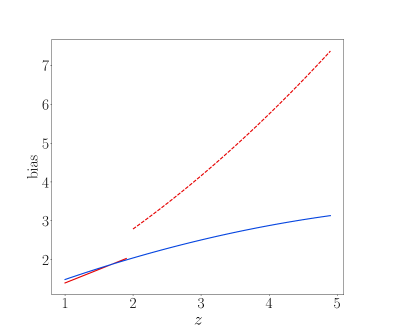
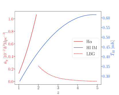
Figure 1: For the galaxy and HI IM surveys: clustering biases (left panel); comoving number densities (right panel, red, left-hand $y$-axis) and HI IM temperature (blue, right-hand $y$-axis).

3.1 Noise

For galaxy surveys, $g={\rm H}\alpha$ or LBG, the shot noise is assumed to be Poissonian, so that the total observed auto-power is

$$\tilde{P}_{g}(z,k,\mu)=P_{g}(z,k,\mu)+\frac{1}{\bar{n}_{g}(z)}\;.$$ (3.7)

In HI IM surveys, HI = H or P, the dominant noise on linear scales is the thermal (or instrumental) noise [39, 35], so that shot noise can safely be neglected and the observed HI IM power spectrum is

$$\tilde{P}_{\rm HI}(z,k,\mu)=P_{\rm HI}(z,k,\mu)+P_{\rm HI}^{\mathrm{therm}}(z,k,\mu)\;,$$ (3.8)

where $P_{\rm HI}^{\mathrm{therm}}$ depends on the model of the sky temperature in the radio band, the survey specifications and the survey mode (single-dish or interferometer). For the interferometer (IF) mode that we consider, the thermal noise power spectrum is [40, 41, 42, 43]:

$$P_{\rm HI}^{\mathrm{therm}}(z,k_{\perp})=\frac{\Omega_{\mathrm{sky}}}{2\nu_{21}t_{\mathrm{tot}}}\,\frac{(1+z)r(z)^{2}}{\mathcal{H}(z)}\,\left[\frac{T_{\mathrm{sys}}(z)}{\bar{T}_{\rm HI}(z)}\right]^{2}\,\left[\frac{\lambda_{21}(1+z)}{A_{\mathrm{e}}}\right]^{2}\frac{1}{n^{\mathrm{phys}}_{\mathrm{b}}(z,k_{\perp})}{\frac{1}{\theta_{\rm fov}(z)^{2}}}\;,$$ (3.9)

where $k_{\perp}=k\sqrt{1-\mu^{2}}$ is the transverse mode, $\nu_{21}=1420\,\mathrm{MHz}$ is the rest-frame frequency of the $\lambda_{21}=21\,$cm emission, $t_{\mathrm{tot}}$ is the total observing time, $r$ is the radial comoving distance, $\mathcal{H}$ is the conformal Hubble rate, $n^{\mathrm{phys}}_{\mathrm{b}}$ is the physical baseline density of the array distribution (see below). The effective beam area is

$$A_{\mathrm{e}}=0.7\,\frac{\pi}{4}D_{\mathrm{d}}^{2}\;,$$ (3.10)

with dish diameter $D_{\mathrm{d}}$ and the field of view is

$$\theta_{\rm fov}(z)=1.22\,\frac{\lambda_{21}(1+z)}{D_{\rm d}}\;.$$ (3.11)

For a given baseline of length $L$, we use the fitting formula for close-packed arrays given in [42] (see also [44, 43]):

$$n^{\mathrm{phys}}_{\mathrm{b}}(z,k_{\perp})=\left(\frac{N_{\mathrm{s}}}{D_{\mathrm{d}}}\right)^{2}\frac{a+b(L/L_{\mathrm{s}})}{1+c(L/L_{\mathrm{s}})^{d}}\exp{\big{[}-(L/L_{\mathrm{s}})^{e}\big{]}}~{}~{}\text{with}~{}~{}L=\frac{k_{\perp}r(z)}{2\pi}\lambda_{21}(1+z)\,,$$ (3.12)

where $L_{\mathrm{s}}=N_{\mathrm{s}}D_{\mathrm{d}}$. H is a square close-packed array, while P is a hexagonal close-packed array with 50% fill factor. This means that half the dish sites are randomly empty, so the array is equivalent in size to that of twice the number of elements but with a quarter of the baseline density [44]. Then it follows that $N_{\rm s}^{2}=N_{\rm d}$ for H and $N_{\rm s}^{2}=2N_{\rm d}$ for P [42, 45]. The values of the parameters are given in Table 1.

The baseline densities for the H and P surveys are shown in Figure 2. Note that the thermal noise, which is $\propto 1/n_{\rm b}^{\rm phys}$, tends to infinity at the maximum baseline $D_{\rm max}$.

Table 1: Specifications of HI IM surveys.

Survey	$N_{\mathrm{d}}$	$N_{\mathrm{s}}$	$t_{\rm tot}$	$T_{\mathrm{d}}$	$D_{\mathrm{d}}$	$D_{\mathrm{max}}$
			[$10^{3}\rm{hr}$]	[K]	[m]	[m]
H256  (1024)	256 (1024)	16 (32)	12	50	6	141  (282)
P5k    (32k)	5k (32k)	100 (253)	20	93	6	648  (1640)
Fitting	$a$	$b$	$c$	$d$	$e$
parameters
H256  (1024)	0.4847	-0.3300	1.3157	1.5974	6.8390
P5k    (32k)	0.5698	-0.5274	0.8358	1.6635	7.3177

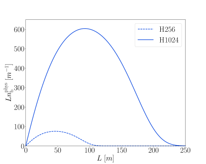
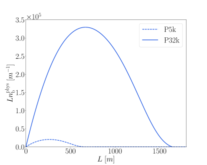
Figure 2: Physical baseline density for HI IM surveys H1024 (left) and P32k (right).

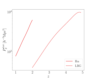
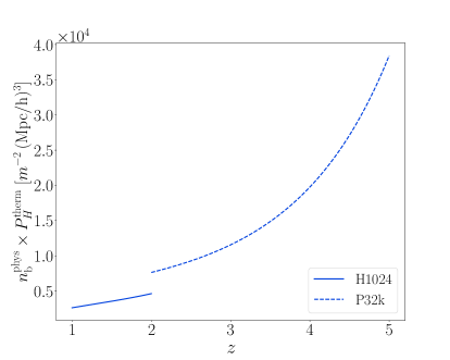
Figure 3: Redshift evolution of galaxy shot noise (left) and HI IM thermal noise times physical baseline density (right).

The system temperature is modelled as [42]:

$$T_{\mathrm{sys}}(z)=T_{\rm d}(z)+T_{\rm sky}(z)=T_{\rm d}+2.7+25\bigg{[}\frac{400\,\mathrm{MHz}}{\nu_{21}}(1+z)\bigg{]}^{2.75}~{}\mathrm{K},$$ (3.13)

where $T_{\rm d}$ is the dish receiver temperature, given in Table 1.

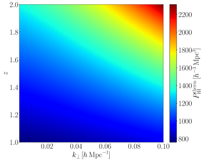
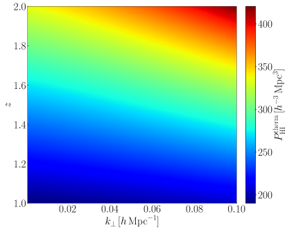
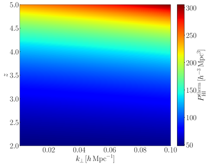
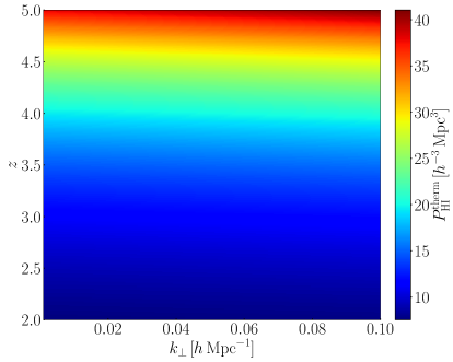
Figure 4: 2D colour plot of thermal noise for HI IM surveys: H256 (top left), H1024 (top right), P5k (bottom left) and P32k (bottom right).

The cross-noise power spectrum between HI IM and galaxy surveys depends on the extent of overlapping halos that host the HI emitters and the galaxies. Typically it is neglected, as motivated in [46, 47]. Then the observed cross-power spectra are

$$\tilde{P}_{g{\rm HI}}=P_{g{\rm HI}}\,.$$ (3.14)

The noise auto-power for all surveys is shown in Figure 3.

3.2 HI IM foreground avoidance

HI IM surveys are contaminated by foregrounds that are much larger than the HI signal. The cleaning of foregrounds from the HI signal relies on the fact that the foregrounds are nearly spectrally smooth (see e.g. [48, 49] and references there in for recent advances). However, the cleaning is not perfect, and in some regions of Fourier space the signal loss is large. For simplified Fisher forecasts, we assume that cleaning is successful, except in the known regions of Fourier space where cleaning is expected to be least effective. Then we use foreground filters that avoid these regions. There are two regions of foreground avoidance for IF-mode surveys.

1. We filter out long-wavelength radial modes with $|k_{\parallel}|\lesssim k_{\rm fg}$, where $k_{\rm fg}$ is a suitable minimum radial mode for future surveys. We follow [50] and use the radial damping factor

   $${\cal D}_{\rm fg}(k,\mu)=1-\exp\bigg{[}-\bigg{(}\frac{k_{\parallel}}{k_{\rm fg}}\bigg{)}^{\!\!{2}\,}\bigg{]}~{}~{}\text{with}~{}~{}k_{\rm fg}=0.005~{}h{\rm Mpc}^{-1}\;.$$ (3.15)

2. A physical baseline in the IF array probes different angular scales $k_{\perp}$ at different frequencies (and hence different $z$). As a consequence, monochromatic emission from a foreground point source can contaminate the signal in a wedge-shaped region of Fourier space [51, 52]. This contamination occurs within $N_{\rm w}$ primary beams of a pointing, where $N_{\rm w}=0$ is the ideal case of no contamination, which occurs in principle if calibration of the interferometer is near-perfect [53]. Currently this precision in calibration and stability is not achievable. In order to avoid the wedge region we therefore impose the filter [51, 52, 54, 41, 42]

   $$\left|k_{\parallel}\right|>A_{\mathrm{w}}(z)\,k_{\perp}\quad\text{where}\quad A_{\mathrm{w}}(z)=r(z)\mathcal{H}(z)\sin\big{[}0.61N_{\mathrm{w}}\,\theta_{\mathrm{fov}}(z)\big{]}\;.$$ (3.16)

   In our forecasts we take $N_{\mathrm{w}}=1$.

Figure 5 illustrates ${\cal D}_{\rm fg}$ and $A_{\mathrm{w}}$. Foreground filters lead to the following modifications of the power spectra:

$$P_{A{\rm HI}}(z,{k},\mu) \rightarrow {\cal D}_{\rm fg}(k,\mu)\,\Theta\big{(}\left|k_{\parallel}\right|-A_{\mathrm{w}}(z)k_{\perp}\big{)}\,P_{A{\rm HI}}(z,{k},\mu)\,,$$ (3.17)

where $A=\,$HI or H$\alpha$ or LBG, and $\Theta$ is the Heaviside step function.

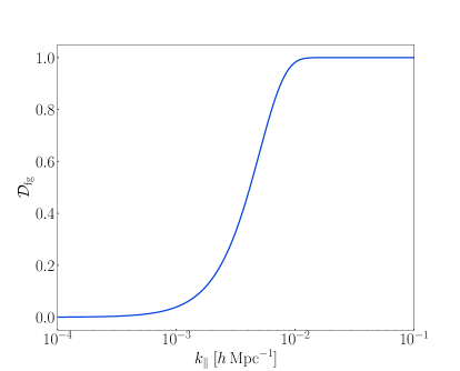
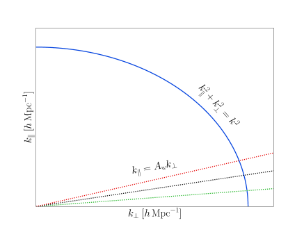
Figure 5: Radial foreground damping function (left). Schematic to illustrate the foreground wedge; the wedge angle increases with redshift (right).

3.3 Maximum and minimum scales

Since the local PNG signal in power spectra is on ultra-large scales, we only require linear perturbation theory. This means that we can exclude scales where linear perturbations break down, i.e. $k<k_{\mathrm{max}}$, where [55, 56, 57, 58]

$$k_{\mathrm{max}}(z)=k_{\mathrm{max},0}\big{(}1+z\big{)}^{2/(2+n_{s})}\;.$$ (3.18)

Then we choose a very conservative value of $k_{\mathrm{max},0}=0.08\;h\,\mathrm{Mpc}^{-1}$.

The minimum wavenumber $k_{\mathrm{min}}$ in each redshift bin is the fundamental mode $k_{\mathrm{f}}$, given by the comoving volume of the bin of width $\Delta z$ centered at $z$:

$$k_{\mathrm{min}}(z)=k_{\mathrm{f}}(z)=\frac{2\pi}{V(z)^{1/3}}\quad\text{with}\quad V(z)=\frac{\Omega_{\mathrm{sky}}}{3}\Big{[}r\big{(}z+\Delta z/2\big{)}^{3}-r\big{(}z-\Delta z/2\big{)}^{3}\Big{]}\;.$$ (3.19)

The minimum and maximum scales are shown in Figure 6.

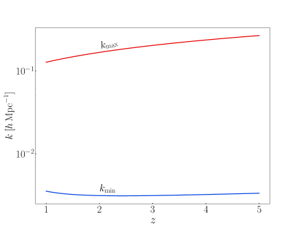
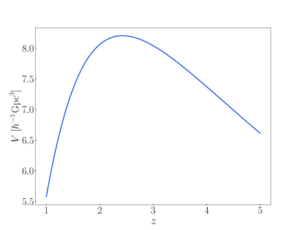
Figure 6: Minimum and maximum wavenumbers (left) and comoving volume (right) over the redshift range of the surveys.

4 Fisher forecast

For a given redshift bin, the multi-tracer Fisher matrix for the combination of two dark matter tracers $g$ and HI is

$$F_{\alpha\beta}^{\bm{P}}=\sum_{\mu=-1}^{+1}\,\sum_{k=k_{\mathrm{min}}}^{k_{\mathrm{max}}}\,\partial_{\alpha}\,\bm{P}\cdot\mathrm{Cov}(\bm{P},\bm{P})^{-1}\cdot\partial_{\beta}\,\bm{P}^{\mathrm{T}}\;,$$ (4.1)

where $\partial_{\alpha}=\partial\,/\,\partial\vartheta_{\alpha}$. Here $\bm{P}$ is the data vector of the power spectra,

$$\bm{P}=\big{(}P_{g}\,,\,P_{g{\rm HI}}\,,\,P_{\rm HI}\big{)}\;.$$ (4.2)

Note that the noise is excluded since it is independent of the cosmological and nuisance parameters. The noise enters the covariance [59, 60, 61, 62]:

$$\mathrm{Cov}(\bm{P},\bm{P})=\frac{k_{\rm f}^{3}}{4\pi k^{2}\Delta k}\,\frac{2}{\Delta\mu}\,\begin{pmatrix}\tilde{P}_{g}^{2}&&\tilde{P}_{g}\tilde{P}_{g{\rm HI}}&&\tilde{P}_{g{\rm HI}}^{2}\\ &&&&\\ \tilde{P}_{g}\tilde{P}_{g{\rm HI}}&&\frac{1}{2}\big{(}\tilde{P}_{g}\tilde{P}_{\rm HI}+\tilde{P}_{g{\rm HI}}^{2}\big{)}&&\tilde{P}_{\rm HI}\tilde{P}_{g{\rm HI}}\\ &&&&\\ \tilde{P}_{g{\rm HI}}^{2}&&\tilde{P}_{\rm HI}\tilde{P}_{g{\rm HI}}&&\tilde{P}_{\rm HI}^{2}\end{pmatrix}\;.$$ (4.3)

Here $\Delta k$ and $\Delta\mu$ are the bin-widths for $k$ and $\mu$, which we choose following [63, 64]:

$$\Delta\mu=0.04\quad\text{and}\quad\Delta k=k_{\mathrm{f}}\;.$$ (4.4)

In this paper our focus is on the improvements that the multi-tracer can deliver for pairs (galaxy, HI IM) of high and very high redshift surveys. We assume that most of the cosmological parameters have been measured by surveys that focus on medium to small scales. Since $f_{\mathrm{NL}}$ affects the amplitude and shape of the power spectrum on ultra-large scales, we include in the Fisher analysis the cosmological parameters $A_{s}$ and $n_{s}$ that directly affect these properties of the power spectrum. We further assume that (a) $\bar{T}_{\rm HI}$, (b) the redshift evolution of the Guassian clustering biases $b_{A}$, and (c) the degeneracies between $b_{A}$ and $A_{s}$ and between $\bar{T}_{\rm HI}$ and $A_{s}$, have been broken by other surveys that focus on medium to small scales. Then we consider the following cosmological and nuisance parameters:

$$\vartheta_{\alpha}=\big{(}f_{\mathrm{NL}},\;A_{s},\;n_{s},\;b_{g0},\;b_{{\rm HI}0}\big{)}\,.$$ (4.5)

The fiducial values for the LCDM cosmological parameters are taken from Planck [65] and we assume $\bar{f}_{\rm NL}=0$.

Derivatives for $f_{\mathrm{NL}}$, $A_{s}$ and $b_{A0}$ are computed analytically, while the $n_{s}$ derivative is computed using the 5-point stencil method, with step-length 0.1 [66].

The Fisher forecast results are shown in Figure 7 and Figure 8, which display the $1\sigma$ error contours for the multi-tracer pairs $(A,B)=({\rm H}\alpha$, H) and (LBG, P), where we have marginalised over the bias nuisance parameters. The numerical values of $\sigma(f_{\rm NL})$ are shown in Table 2.

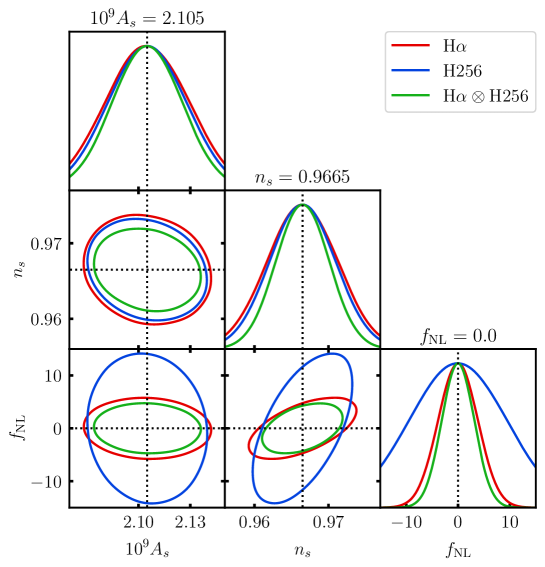
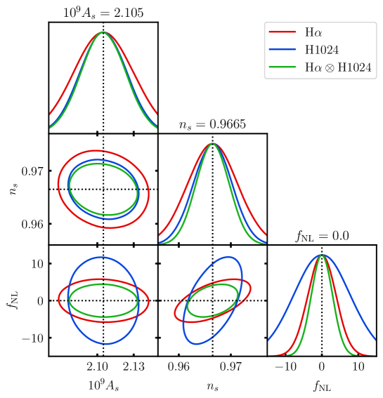
Figure 7: 1$\sigma$ marginalised contours for cosmological parameters from the H$\alpha$ and H surveys.

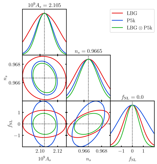
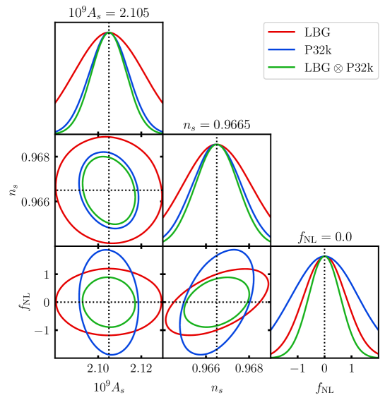
Figure 8: 1$\sigma$ marginalised contours for cosmological parameters from the LBG and P surveys.

Table 2: Marginalised errors on $f_{\mathrm{NL}}$. Final column shows the percentage improvement in precision for each single tracer from the multi-tracer.

Surveys $A,\,A\otimes B$	$\sigma(f_{\mathrm{NL}})$	$\big{[}\sigma(A)-\sigma(A\otimes B)\big{]}/\sigma(A)$
		$\times 100\%$
H$\alpha$	3.83	18  (24)
LBG	0.787	23  (25)
H256  (1024)	9.42  (7.74)	68  (62)
P5k    (32k)	1.31  (1.24)	54  (52)
H$\alpha$ $\otimes$ H256   (1024)	3.13    (2.92)
LBG $\otimes$ P5k  (32k)	0.606  (0.591)

5 Conclusion

Our Fisher analysis shows the effectiveness of combining tracers to enhance the precision in future measurements of local PNG. The multi-tracer also improves precision on $n_{s}$ and $A_{s}$. It is noticeable that the HI IM surveys provide stronger constraints on $n_{s},A_{s}$ than the galaxy surveys, while the reverse is true for $f_{\rm NL}$. The reason is that the $n_{s},A_{s}$ signals are mainly dependent on medium scales, while the $f_{\rm NL}$ signal is based on ultra-large scales. The HI IM IF-mode surveys provide better constraints on medium scales than the galaxy surveys. However, on ultra-large scales these surveys lose constraining power due to the foreground filters.

Our assumption on the halo-dependent PNG bias, i.e. that $b_{A\phi}\propto b_{A}-p_{A}$ as in (2.7) and (2.8), also affects galaxies and HI IM differently. In the simplest universality model, $p_{A}=1$, there is no difference between galaxies and HI IM in the form of the PNG bias. In our case, since $p_{g}<1$, it follows that $b_{A\phi}$ is larger than in the $p=1$ model. Consequently, the constraints for galaxy surveys on $f_{\rm NL}$ are improved compared to $p=1$. By contrast, $p_{\rm HI}>1$ means that $f_{\rm NL}$ constraints are degraded for HI IM surveys compared to $p=1$.

Single-tracer Fisher constraints for surveys similar to our mock surveys have been computed previously: e.g., [67] for Euclid; [34] for MegaMapper and PUMA; [44] for HIRAX and PUMA. These constraints are qualitatively compatible with ours – taking into account the following differences:

• Previous work uses the universality model for $b_{A\phi}$, while we use (2.7) and (2.8).

• Our mock surveys have differences in the redshift range, sky area and observing time (for HI IM) compared to the surveys considered in previous work.

• There are differences amongst the previous works, and with our paper, in the cosmological and nuisance parameters that are used and marginalised over.

Previous works, to our knowledge, do not treat the multi-tracer pairs that we analyse, so that comparisons of our multi-tracer results with previous results is not possible. Table 2 shows (final column) the improvement in precision from the multi-tracer combinations for each single tracer case: this ranges from $\sim 20$ to $\sim 70\%$. The best single-tracer and multi-tracer $f_{\mathrm{NL}}$ precision is delivered at the highest redshifts, by LBG and LBG$\,\otimes\,$P (Figure 8). The LBG survey on its own already achieves $\sigma(f_{\mathrm{NL}})<1$ (this is compatible with [34]), while P constraints (which are compatible with [44]) are weaker because of foreground contamination on ultra-large scales. When LBG and P are combined, we achieve an improvement in $\sigma(f_{\mathrm{NL}})$ of $\gtrsim 50\%$ when compared to the single-tracer P, and $\gtrsim 20\%$ when compared to the single-tracer LBG.

Regarding foreground avoidance filters, we have used the following values for the radial long-wavelength mode limit and the wedge primary beam number:

$$k_{\rm fg}=0.005\,h{\rm Mpc}^{-1}\,,\quad N_{\rm w}=1\,.$$ (5.1)

Although this is fairly optimistic compared to some previous treatments, it should be noted that further advances in foreground treatments will emerge. In particular:

• density reconstruction methods, such as forward model reconstruction, are being developed to retrieve the long wavelength modes lost to foregrounds (e.g [68, 58, 69]);

• advances in the stability and calibration of interferometers will reduce the impact of the wedge and in principle will be able in future to reduce its impact to negligible.

Our Fisher forecasts are of course highly simplified compared to observational and data reality. In practice there are numerous systematics to be modelled and there are major data constraints on the simulations necessary to build a data pipeline. Nevertheless, the simplified Fisher analysis has shown that multi-tracing galaxy and intensity HI IM surveys at high to very high redshifts is worth exploring further. Furthermore, the multi-tracer will alleviate the impact of nuisance parameters and systematics in the galaxy and HI IM samples.

Finally, we note that our forecasts use a plane-parallel approximation in the Fourier power spectra. Future work will relax this assumption by including wide-angle effects (see e.g. [70, 71, 72]).

Acknowledgements
We thank Dionysios Karagiannis, Stefano Camera and Lazare Guedezounme for very helpful comments. We are supported by the South African Radio Astronomy Observatory (SARAO) and the National Research Foundation (Grant No. 75415).

References

- [1] A. Achúcarro et al., Inflation: Theory and Observations, arXiv:2203.08128.
- [2] R. de Putter, J. Gleyzes, and O. Doré, Next non-Gaussianity frontier: What can a measurement with (fNL)1 tell us about multifield inflation?, Phys. Rev. D 95 (2017), no. 12 123507, [arXiv:1612.05248].
- [3] P. D. Meerburg et al., Primordial Non-Gaussianity, Bull. Am. Astron. Soc. 51 (2019), no. 3 107, [arXiv:1903.04409].
- [4] Planck Collaboration, Y. Akrami et al., Planck 2018 results. IX. Constraints on primordial non-Gaussianity, Astron. Astrophys. 641 (2020) A9, [arXiv:1905.05697].
- [5] N. Dalal, O. Dore, D. Huterer, and A. Shirokov, The imprints of primordial non-gaussianities on large-scale structure: scale dependent bias and abundance of virialized objects, Phys. Rev. D77 (2008) 123514, [arXiv:0710.4560].
- [6] S. Matarrese and L. Verde, The effect of primordial non-Gaussianity on halo bias, Astrophys. J. Lett. 677 (2008) L77–L80, [arXiv:0801.4826].
- [7] A. Raccanelli, F. Montanari, D. Bertacca, O. Doré, and R. Durrer, Cosmological Measurements with General Relativistic Galaxy Correlations, JCAP 05 (2016) 009, [arXiv:1505.06179].
- [8] D. Alonso, P. Bull, P. G. Ferreira, R. Maartens, and M. Santos, Ultra large-scale cosmology in next-generation experiments with single tracers, Astrophys. J. 814 (2015) 145, [arXiv:1505.07596].
- [9] U. Seljak, Extracting primordial non-gaussianity without cosmic variance, Phys. Rev. Lett. 102 (2009) 021302, [arXiv:0807.1770].
- [10] P. McDonald and U. Seljak, How to measure redshift-space distortions without sample variance, JCAP 10 (2009) 007, [arXiv:0810.0323].
- [11] N. Hamaus, U. Seljak, and V. Desjacques, Optimal Constraints on Local Primordial Non-Gaussianity from the Two-Point Statistics of Large-Scale Structure, Phys. Rev. D 84 (2011) 083509, [arXiv:1104.2321].
- [12] L. R. Abramo and K. E. Leonard, Why multi-tracer surveys beat cosmic variance, Mon. Not. Roy. Astron. Soc. 432 (2013) 318, [arXiv:1302.5444].
- [13] SKA Collaboration, D. J. Bacon et al., Cosmology with Phase 1 of the Square Kilometre Array: Red Book 2018: Technical specifications and performance forecasts, Publ. Astron. Soc. Austral. 37 (2020) e007, [arXiv:1811.02743].
- [14] Z. Gomes, S. Camera, M. J. Jarvis, C. Hale, and J. Fonseca, Non-Gaussianity constraints using future radio continuum surveys and the multitracer technique, Mon. Not. Roy. Astron. Soc. 492 (2020), no. 1 1513–1522, [arXiv:1912.08362].
- [15] S. Jolicoeur, R. Maartens, and S. Dlamini, Constraining primordial non-Gaussianity by combining next-generation galaxy and 21 cm intensity mapping surveys, Eur. Phys. J. C 83 (2023), no. 4 320, [arXiv:2301.02406].
- [16] D. Alonso and P. G. Ferreira, Constraining ultralarge-scale cosmology with multiple tracers in optical and radio surveys, Phys. Rev. D 92 (2015), no. 6 063525, [arXiv:1507.03550].
- [17] J. Fonseca, S. Camera, M. Santos, and R. Maartens, Hunting down horizon-scale effects with multi-wavelength surveys, Astrophys. J. 812 (2015), no. 2 L22, [arXiv:1507.04605].
- [18] M. Ballardini, W. L. Matthewson, and R. Maartens, Constraining primordial non-Gaussianity using two galaxy surveys and CMB lensing, Mon. Not. Roy. Astron. Soc. 489 (2019), no. 2 1950–1956, [arXiv:1906.04730].
- [19] W. d’Assignies, C. Zhao, J. Yu, and J.-P. Kneib, Cosmological Fisher forecasts for next-generation spectroscopic surveys, Mon. Not. Roy. Astron. Soc. 521 (2023), no. 3 3648, [arXiv:2301.02289].
- [20] M. B. Squarotti, S. Camera, and R. Maartens, Radio-optical synergies at high redshift to constrain primordial non-Gaussianity, arXiv:2307.00058.
- [21] D. Blas, J. Lesgourgues, and T. Tram, The Cosmic Linear Anisotropy Solving System (CLASS) II: Approximation schemes, JCAP 1107 (2011) 034, [arXiv:1104.2933].
- [22] A. Barreira, G. Cabass, F. Schmidt, A. Pillepich, and D. Nelson, Galaxy bias and primordial non-Gaussianity: insights from galaxy formation simulations with IllustrisTNG, JCAP 12 (2020) 013, [arXiv:2006.09368].
- [23] A. Barreira, The local PNG bias of neutral Hydrogen, H, JCAP 04 (2022), no. 04 057, [arXiv:2112.03253].
- [24] A. Barreira, Can we actually constrain fNL using the scale-dependent bias effect? An illustration of the impact of galaxy bias uncertainties using the BOSS DR12 galaxy power spectrum, JCAP 11 (2022) 013, [arXiv:2205.05673].
- [25] A. Barreira and E. Krause, Towards optimal and robust f_nl constraints with multi-tracer analyses, JCAP 10 (2023) 044, [arXiv:2302.09066].
- [26] E. Fondi, L. Verde, F. Villaescusa-Navarro, M. Baldi, W. R. Coulton, G. Jung, D. Karagiannis, M. Liguori, A. Ravenni, and B. D. Wandelt, Taming assembly bias for primordial non-Gaussianity, arXiv:2311.10088.
- [27] A. G. Adame, S. Avila, V. Gonzalez-Perez, G. Yepes, M. Pellejero, C.-H. Chuang, Y. Feng, J. Garcia-Bellido, A. Knebe, and M. S. Wang, PNG-UNITsims: the response of halo clustering to Primodial Non-Gaussianities as a function of mass, arXiv:2312.12405.
- [28] Euclid Collaboration, A. Blanchard et al., Euclid preparation: VII. Forecast validation for Euclid cosmological probes, Astron. Astrophys. 642 (2020) A191, [arXiv:1910.09273].
- [29] L. B. Newburgh et al., HIRAX: A Probe of Dark Energy and Radio Transients, Proc. SPIE Int. Soc. Opt. Eng. 9906 (2016) 99065X, [arXiv:1607.02059].
- [30] D. Crichton et al., Hydrogen Intensity and Real-Time Analysis Experiment: 256-element array status and overview, J. Astron. Telesc. Instrum. Syst. 8 (2022) 011019, [arXiv:2109.13755].
- [31] D. J. Schlegel et al., The MegaMapper: A Stage-5 Spectroscopic Instrument Concept for the Study of Inflation and Dark Energy, arXiv:2209.04322.
- [32] PUMA Collaboration, A. Slosar et al., Packed Ultra-wideband Mapping Array (PUMA): A Radio Telescope for Cosmology and Transients, Bull. Am. Astron. Soc. 51 (2019) 53, [arXiv:1907.12559].
- [33] A. Merson, A. Smith, A. Benson, Y. Wang, and C. M. Baugh, Linear bias forecasts for emission line cosmological surveys, Mon. Not. Roy. Astron. Soc. 486 (2019), no. 4 5737–5765, [arXiv:1903.02030].
- [34] N. Sailer, E. Castorina, S. Ferraro, and M. White, Cosmology at high redshift – a probe of fundamental physics, JCAP 12 (2021), no. 12 049, [arXiv:2106.09713].
- [35] F. Villaescusa-Navarro et al., Ingredients for 21 cm Intensity Mapping, Astrophys. J. 866 (2018), no. 2 135, [arXiv:1804.09180].
- [36] R. Maartens, J. Fonseca, S. Camera, S. Jolicoeur, J.-A. Viljoen, and C. Clarkson, Magnification and evolution biases in large-scale structure surveys, JCAP 12 (2021), no. 12 009, [arXiv:2107.13401].
- [37] S. Ferraro et al., Inflation and Dark Energy from Spectroscopy at , Bull. Am. Astron. Soc. 51 (2019), no. 3 72, [arXiv:1903.09208].
- [38] MeerKLASS Collaboration, M. G. Santos et al., MeerKLASS: MeerKAT Large Area Synoptic Survey, in MeerKAT Science: On the Pathway to the SKA, 9, 2017. arXiv:1709.06099.
- [39] E. Castorina and F. Villaescusa-Navarro, On the spatial distribution of neutral hydrogen in the Universe: bias and shot-noise of the HI power spectrum, Mon. Not. Roy. Astron. Soc. 471 (2017), no. 2 1788–1796, [arXiv:1609.05157].
- [40] P. Bull, P. G. Ferreira, P. Patel, and M. G. Santos, Late-time cosmology with 21cm intensity mapping experiments, Astrophys. J. 803 (2015), no. 1 21, [arXiv:1405.1452].
- [41] D. Alonso, P. G. Ferreira, M. J. Jarvis, and K. Moodley, Calibrating photometric redshifts with intensity mapping observations, Phys. Rev. D 96 (2017), no. 4 043515, [arXiv:1704.01941].
- [42] Cosmic Visions 21 cm Collaboration, R. Ansari et al., Inflation and Early Dark Energy with a Stage II Hydrogen Intensity Mapping experiment, arXiv:1810.09572.
- [43] S. Jolicoeur, R. Maartens, E. M. De Weerd, O. Umeh, C. Clarkson, and S. Camera, Detecting the relativistic bispectrum in 21cm intensity maps, JCAP 06 (2021) 039, [arXiv:2009.06197].
- [44] D. Karagiannis, A. Slosar, and M. Liguori, Forecasts on Primordial non-Gaussianity from 21 cm Intensity Mapping experiments, JCAP 11 (2020) 052, [arXiv:1911.03964].
- [45] E. Castorina et al., Packed Ultra-wideband Mapping Array (PUMA): Astro2020 RFI Response, arXiv:2002.05072.
- [46] J.-A. Viljoen, J. Fonseca, and R. Maartens, Constraining the growth rate by combining multiple future surveys, JCAP 09 (2020) 054, [arXiv:2007.04656].
- [47] S. Casas, I. P. Carucci, V. Pettorino, S. Camera, and M. Martinelli, Constraining gravity with synergies between radio and optical cosmological surveys, Phys. Dark Univ. 39 (2023) 101151, [arXiv:2210.05705].
- [48] S. Cunnington, S. Camera, and A. Pourtsidou, The degeneracy between primordial non-Gaussianity and foregrounds in 21 cm intensity mapping experiments, Mon. Not. Roy. Astron. Soc. 499 (2020), no. 3 4054–4067, [arXiv:2007.12126].
- [49] M. Spinelli, I. P. Carucci, S. Cunnington, S. E. Harper, M. O. Irfan, J. Fonseca, A. Pourtsidou, and L. Wolz, SKAO HI intensity mapping: blind foreground subtraction challenge, Mon. Not. Roy. Astron. Soc. 509 (2021), no. 2 2048–2074, [arXiv:2107.10814].
- [50] S. Cunnington, C. Watkinson, and A. Pourtsidou, The H i intensity mapping bispectrum including observational effects, Mon. Not. Roy. Astron. Soc. 507 (2021), no. 2 1623–1639, [arXiv:2102.11153].
- [51] J. C. Pober et al., What Next-Generation 21 cm Power Spectrum Measurements Can Teach Us About the Epoch of Reionization, Astrophys. J. 782 (2014) 66, [arXiv:1310.7031].
- [52] J. C. Pober, The Impact of Foregrounds on Redshift Space Distortion Measurements With the Highly-Redshifted 21 cm Line, Mon. Not. Roy. Astron. Soc. 447 (2015), no. 2 1705–1712, [arXiv:1411.2050].
- [53] A. Ghosh, F. Mertens, and L. V. E. Koopmans, Deconvolving the wedge: maximum-likelihood power spectra via spherical-wave visibility modelling, Mon. Not. Roy. Astron. Soc. 474 (2018), no. 4 4552–4563, [arXiv:1709.06752].
- [54] A. Obuljen, E. Castorina, F. Villaescusa-Navarro, and M. Viel, High-redshift post-reionization cosmology with 21cm intensity mapping, JCAP 05 (2018) 004, [arXiv:1709.07893].
- [55] VIRGO Consortium Collaboration, R. E. Smith, J. A. Peacock, A. Jenkins, S. D. M. White, C. S. Frenk, F. R. Pearce, P. A. Thomas, G. Efstathiou, and H. M. P. Couchmann, Stable clustering, the halo model and nonlinear cosmological power spectra, Mon. Not. Roy. Astron. Soc. 341 (2003) 1311, [astro-ph/0207664].
- [56] R. Maartens, S. Jolicoeur, O. Umeh, E. M. De Weerd, C. Clarkson, and S. Camera, Detecting the relativistic galaxy bispectrum, JCAP 03 (2020), no. 03 065, [arXiv:1911.02398].
- [57] J. Fonseca, J.-A. Viljoen, and R. Maartens, Constraints on the growth rate using the observed galaxy power spectrum, JCAP 1912 (2019), no. 12 028, [arXiv:1907.02975].
- [58] C. Modi, M. White, A. Slosar, and E. Castorina, Reconstructing large-scale structure with neutral hydrogen surveys, JCAP 11 (2019) 023, [arXiv:1907.02330].
- [59] M. White, Y.-S. Song, and W. J. Percival, Forecasting Cosmological Constraints from Redshift Surveys, Mon. Not. Roy. Astron. Soc. 397 (2008) 1348–1354, [arXiv:0810.1518].
- [60] G.-B. Zhao et al., The completed SDSS-IV extended Baryon Oscillation Spectroscopic Survey: a multitracer analysis in Fourier space for measuring the cosmic structure growth and expansion rate, Mon. Not. Roy. Astron. Soc. 504 (2021), no. 1 33–52, [arXiv:2007.09011].
- [61] A. Barreira, On the impact of galaxy bias uncertainties on primordial non-Gaussianity constraints, JCAP 12 (2020) 031, [arXiv:2009.06622].
- [62] D. Karagiannis, R. Maartens, J. Fonseca, S. Camera, and C. Clarkson, Multi-tracer power spectra and bispectra: Formalism, arXiv:2305.04028.
- [63] D. Karagiannis, A. Lazanu, M. Liguori, A. Raccanelli, N. Bartolo, and L. Verde, Constraining primordial non-Gaussianity with bispectrum and power spectrum from upcoming optical and radio surveys, Mon. Not. Roy. Astron. Soc. 478 (2018), no. 1 1341–1376, [arXiv:1801.09280].
- [64] V. Yankelevich and C. Porciani, Cosmological information in the redshift-space bispectrum, Mon. Not. Roy. Astron. Soc. 483 (2019), no. 2 2078–2099, [arXiv:1807.07076].
- [65] Planck Collaboration, N. Aghanim et al., Planck 2018 results. VI. Cosmological parameters, Astron. Astrophys. 641 (2020) A6, [arXiv:1807.06209]. [Erratum: Astron.Astrophys. 652, C4 (2021)].
- [66] S. Yahia-Cherif, A. Blanchard, S. Camera, S. Casas, S. Ilić, K. Markovic, A. Pourtsidou, Z. Sakr, D. Sapone, and I. Tutusaus, Validating the Fisher approach for stage IV spectroscopic surveys, Astron. Astrophys. 649 (2021) A52, [arXiv:2007.01812].
- [67] J.-A. Viljoen, J. Fonseca, and R. Maartens, Multi-wavelength spectroscopic probes: prospects for primordial non-Gaussianity and relativistic effects, JCAP 11 (2021) 010, [arXiv:2107.14057].
- [68] H.-M. Zhu, U.-L. Pen, Y. Yu, and X. Chen, Recovering lost 21 cm radial modes via cosmic tidal reconstruction, Phys. Rev. D 98 (2018), no. 4 043511, [arXiv:1610.07062].
- [69] S. Cunnington et al., The foreground transfer function for H i intensity mapping signal reconstruction: MeerKLASS and precision cosmology applications, Mon. Not. Roy. Astron. Soc. 523 (2023), no. 2 2453–2477, [arXiv:2302.07034].
- [70] J.-A. Viljoen, J. Fonseca, and R. Maartens, Multi-wavelength spectroscopic probes: biases from neglecting light-cone effects, JCAP 12 (2021), no. 12 004, [arXiv:2108.05746].
- [71] M. Noorikuhani and R. Scoccimarro, Wide-angle and relativistic effects in Fourier-space clustering statistics, Phys. Rev. D 107 (2023), no. 8 083528, [arXiv:2207.12383].
- [72] P. Paul, C. Clarkson, and R. Maartens, Wide-angle effects in multi-tracer power spectra with Doppler corrections, JCAP 04 (2023) 067, [arXiv:2208.04819].