Extremal polynomials and polynomial preimages

Abstract.

This article examines the asymptotic behavior of the Widom factors, denoted ${\mathcal{W}}_{n}$, for Chebyshev polynomials of finite unions of Jordan arcs. We prove that, in contrast to Widom’s proposal in [54], when dealing with a single smooth Jordan arc, ${\mathcal{W}}_{n}$ converges to 2 exclusively when the arc is a straight line segment. Our main focus is on analysing polynomial preimages of the interval $[-2,2]$, and we provide a complete description of the asymptotic behavior of ${\mathcal{W}}_{n}$ for symmetric star graphs and quadratic preimages of $[-2,2]$. We observe that in the case of star graphs, the Chebyshev polynomials and the polynomials orthogonal with respect to equilibrium measure share the same norm asymptotics, suggesting a potential extension of the conjecture posed in [18]. Lastly, we propose a possible connection between the $S$-property and Widom factors converging to $2$.

Keywords Chebyshev polynomials, Widom factors, polynomial preimages, star graphs

Mathematics Subject Classification 41A50, 30C10, 26D05

1. Introduction

Let ${\mathsf{E}}$ be a compact subset of ${\mathbb{C}}$ with at least $n+1$ points. The $n$th Chebyshev polynomial of ${\mathsf{E}}$, denoted $T_{n}^{\mathsf{E}}$, is the unique monic polynomial of degree $n$ which minimises the supremum norm on ${\mathsf{E}}$. In other words, $T_{n}^{\mathsf{E}}$ is the polynomial

$$T_{n}^{\mathsf{E}}(z)=z^{n}+\sum_{k=0}^{n-1}a_{k}z^{k}$$

which satisfies

$$\|T_{n}^{\mathsf{E}}\|_{\mathsf{E}}:=\max_{z\in{\mathsf{E}}}|T_{n}^{{\mathsf{E}}}(z)|=\min_{b_{0},b_{1},\ldots,b_{n-1}\in{\mathbb{C}}}\max_{z\in{\mathsf{E}}}\left|z^{n}+\sum_{k=0}^{n-1}b_{k}z^{k}\right|.$$

Facts regarding existence and uniqueness of $T_{n}^{\mathsf{E}}$ can be found in, e.g., [42, 30]. See also [14, 17] for a recent account on the basic theory of Chebyshev polynomials. These polynomials were initially studied by Chebyshev [12, 13] in the case where ${\mathsf{E}}=[-1,1]$. In this situation, he showed that the polynomials are explicitly given by the formula

$$T_{n}(x):=T_{n}^{[-1,1]}(x)=2^{1-n}\cos\bigl{(}n\arccos(x)\bigr{)},\quad|x|\leq 1.$$ (1.1)

This representation further hints at a property of the Chebyshev polynomials that holds for arbitrary compact subsets of the real line. A monic degree $n$ polynomial, $P_{n}$, is the Chebyshev polynomial of ${\mathsf{E}}\subset{\mathbb{R}}$ if and only if there exists points $x_{0}<x_{1}<\ldots<x_{n}$ in ${\mathsf{E}}$ such that

$$P_{n}(x_{k})=(-1)^{n-k}\|P_{n}\|_{\mathsf{E}},\quad k=0,1,\ldots,n.$$

This characterising property of the Chebyshev polynomials is called alternation and one can use it to prove several facts concerning their asymptotic behaviour (see, e.g., [14, 15]).

It should be noted that alternation fails to hold for Chebyshev polynomials of non-real compact subsets of ${\mathbb{C}}$. Instead, the asymptotics of such polynomials is typically studied using potential theoretic methods. This is an approach dating back to Faber [20], Fekete [21], and Szegő [47]. Faber investigated Chebyshev polynomials by constructing trial polynomials, the so-called Faber polynomials, from the associated conformal map which maps the exterior of ${\mathsf{E}}$ to the exterior of the closed unit disk, $\overline{{\mathbb{D}}}$. Of course, the existence of this conformal map assumes that the complement of ${\mathsf{E}}$ is simply connected on the Riemann sphere.

As for notation, let $\overline{{\mathbb{C}}}$ denote the Riemann sphere ${\mathbb{C}}\cup\{\infty\}$. Throughout the paper, we shall make use of the following important notions

• $\operatorname{Cap}({\mathsf{E}})$, the logarithmic capacity of ${\mathsf{E}}$

• $G_{\mathsf{E}}(\,\cdot\,):=G_{{\mathsf{E}}}(\,\cdot\,,\infty)$, the Green’s function for $\overline{{\mathbb{C}}}\setminus{\mathsf{E}}$ with pole at $\infty$

• $\mu_{\mathsf{E}}$, the equilibrium measure of ${\mathsf{E}}$

Recall also the relation

$$\int\log|x-z|\,d\mu_{\mathsf{E}}(x)=G_{\mathsf{E}}(z)+\log\operatorname{Cap}({\mathsf{E}}).$$ (1.2)

For a more in depth account of potential theory, we refer the reader to, e.g., [7, 23, 25, 29, 35].

1.1. Widom factors for $T_{n}^{\mathsf{E}}$

One way of quantatively describing the norm of the Chebyshev polynomials using logarithmic capacity is via the Faber–Fekete–Szegő theorem which states that

$$\lim_{n\rightarrow\infty}\|T_{n}^{{\mathsf{E}}}\|_{\mathsf{E}}^{1/n}=\operatorname{Cap}({\mathsf{E}})$$ (1.3)

for any compact set ${\mathsf{E}}\subset{\mathbb{C}}$ (see, e.g., [35, Chapter 5.5]). This implies that $\operatorname{Cap}({\mathsf{E}})^{n}$ is the leading order behaviour of $\|T_{n}^{{\mathsf{E}}}\|_{{\mathsf{E}}}$, and (1.3) limits the way that the so-called Widom factors defined by

$${\mathcal{W}}_{n,\infty}({\mathsf{E}}):=\frac{\|T_{n}^{\mathsf{E}}\|_{\mathsf{E}}}{\operatorname{Cap}({\mathsf{E}})^{n}}$$ (1.4)

can grow as $n$ increases. For a wide variety of sets, this quantity is known to be bounded in $n$ and its asymptotic behaviour is of particular interest. See, e.g., [5, 6, 17] for more details.

Another classical result in the theory of Chebyshev polynomials is

Theorem.

Let ${\mathsf{E}}\subset{\mathbb{C}}$ be a compact set. Then

$$\|T_{n}^{\mathsf{E}}\|_{\mathsf{E}}\geq\operatorname{Cap}({\mathsf{E}})^{n}$$ (1.5)

and if ${\mathsf{E}}\subset{\mathbb{R}}$, we even have

$$\|T_{n}^{\mathsf{E}}\|_{\mathsf{E}}\geq 2\operatorname{Cap}({\mathsf{E}})^{n}.$$ (1.6)

While (1.5) goes back to Szegő [47], the inequality in (1.6) is more recent and due to Schiefermayr [38]. We shall present a proof of these statements below. Partly because our method will be used in later parts of the paper and is much shorter than the one presented in [38], and partly for completeness. Our proof rests on the following formula for capacity of polynomial preimages.

Lemma.

Let ${\mathsf{E}}$ be a compact subset of ${\mathbb{C}}$ and suppose $P(z)=\sum_{k=0}^{m}a_{k}z^{k}$ is a polynomial with $a_{m}\neq 0$. If

$${\mathsf{E}}_{P}:=\bigl{\{}z:P(z)\in{\mathsf{E}}\bigr{\}}=P^{-1}({\mathsf{E}}),$$

then

$$G_{{\mathsf{E}}_{P}}(z)=\frac{1}{m}G_{\mathsf{E}}\bigl{(}P(z)\bigr{)}\quad\text{and}\quad\operatorname{Cap}({\mathsf{E}}_{P})=\left(\frac{\operatorname{Cap}({\mathsf{E}})}{|a_{m}|}\right)^{1/m}.$$ (1.7)

For a proof of this fact, see [35, Theorem 5.2.5].

Proof of theorem.

Let ${\mathsf{E}}\subset{\mathbb{C}}$ be an arbitrary compact set. Clearly,

$${\mathsf{E}}\subset(T_{n}^{\mathsf{E}})^{-1}\Big{(}\bigl{\{}z:|z|\leq\|T_{n}^{{\mathsf{E}}}\|_{{\mathsf{E}}}\bigr{\}}\Big{)}.$$

Applying (1.7) together with the facts that $\operatorname{Cap}$ is monotone with respect to set inclusion and a disk of radius $r>0$ has capacity equal to $r$, we obtain that

$$\operatorname{Cap}({\mathsf{E}})\leq\operatorname{Cap}\Big{(}\bigl{\{}z:|z|\leq\|T_{n}^{{\mathsf{E}}}\|_{{\mathsf{E}}}\bigr{\}}\Big{)}^{1/n}=\|T_{n}^{{\mathsf{E}}}\|^{1/n}.$$

This proves (1.5).

If ${\mathsf{E}}\subset{\mathbb{R}}$, then $T_{n}^{{\mathsf{E}}}$ is easily shown to have only real coefficients. Hence

$${\mathsf{E}}\subset(T_{n}^{\mathsf{E}})^{-1}\Big{(}\bigl{\{}z:z\in\bigl{[}-\|T_{n}^{\mathsf{E}}\|_{\mathsf{E}},\|T_{n}^{{\mathsf{E}}}\|_{\mathsf{E}}\bigr{]}\bigr{\}}\Big{)}.$$

As the capacity of an interval $[a,b]$ equals ${(b-a)}/{4}$, yet another application of (1.7) implies that

$$\operatorname{Cap}({\mathsf{E}})\leq\operatorname{Cap}\Big{(}\bigl{\{}z:z\in\bigl{[}-\|T_{n}^{\mathsf{E}}\|_{\mathsf{E}},\|T_{n}^{{\mathsf{E}}}\|_{\mathsf{E}}\bigr{]}\bigr{\}}\Big{)}^{1/n}=\left(\frac{\|T_{n}^{\mathsf{E}}\|_{\mathsf{E}}}{2}\right)^{1/n},$$

proving (1.6). ∎

Remark.

Note that the above theorem can be restated in terms of the Widom factors as

$${\mathcal{W}}_{n,\infty}({\mathsf{E}})\geq 1\;\text{ for }\;{\mathsf{E}}\subset{\mathbb{C}}$$ (1.8)

and

$${\mathcal{W}}_{n,\infty}({\mathsf{E}})\geq 2\;\text{ when }\;{\mathsf{E}}\subset{\mathbb{R}}.$$ (1.9)

The sets for which the Szegő lower bound (1.5) is saturated for some value of $n$ were determined in [16]. With $O\partial(\,\cdot\,)$ denoting the outer boundary and $\partial{\mathbb{D}}$ the unit circle, the authors proved that

$${\mathcal{W}}_{n,\infty}({\mathsf{E}})=1\quad\text{if and only if }\quad O\partial({\mathsf{E}})=P^{-1}(\partial\mathbb{D})$$

for some polynomial $P$ of degree $n$. Regarding Schiefermayr’s lower bound, it was proven in [51] (see also [16]) that for ${\mathsf{E}}\subset{\mathbb{R}}$,

$${\mathcal{W}}_{n,\infty}({\mathsf{E}})=2\quad\text{if and only if }\quad{\mathsf{E}}=P^{-1}\bigl{(}[-2,2]\bigr{)}$$ (1.10)

for some degree $n$ polynomial $P$.

Now the question remains in which cases we have an asymptotic saturation of these lower bounds. More precisely, when does it happen that

$$\lim_{n\rightarrow\infty}{\mathcal{W}}_{n,\infty}({\mathsf{E}})=1\text{ or }2?$$

It is known that if ${\mathsf{E}}$ is the closure of a Jordan domain with boundary curve of class $C^{2+\epsilon}$ (i.e., its coordinates are $C^{2+\epsilon}$ functions of arc length), then

$$\lim_{n\rightarrow\infty}{\mathcal{W}}_{n,\infty}({\mathsf{E}})=1.$$ (1.11)

This was first shown in the case where ${\mathsf{E}}$ has analytic boundary by Faber [20] and then extended to the case where the boundary curve is of class $C^{2+\epsilon}$ by Widom [54]. However, there may well be many other connected sets ${\mathsf{E}}\subset{\mathbb{C}}$ for which (1.11) holds.

For ${\mathsf{E}}\subset{\mathbb{R}}$, Totik [52] completely characterised the sets which asymptotically saturate the Schiefermayr lower bound (1.6). He proved that

$$\lim_{n\rightarrow\infty}{\mathcal{W}}_{n,\infty}({\mathsf{E}})=2$$ (1.12)

if and only if ${\mathsf{E}}$ is an interval, in which case ${\mathcal{W}}_{n,\infty}({\mathsf{E}})=2$ for every $n$.

One may ask — and this is a main point of the present article — if there are more subsets ${\mathsf{E}}\subset{\mathbb{C}}$ for which (1.12) holds true. Widom [54] conjectured that any sufficiently nice set which contains an arc component should satisfy (1.12). However, this was shown to be false even in the case of Jordan arcs. In particular, Thiran and Detaille [50] observed that if ${\mathsf{E}}_{\alpha}=\{z:|z|=1,\,|\arg z|\leq\alpha\}$ with $\alpha\in(0,\pi)$, then

$$\lim_{n\rightarrow\infty}{\mathcal{W}}_{n,\infty}({\mathsf{E}}_{\alpha})=2\cos^{2}\left(\alpha/4\right)<2.$$ (1.13)

See also [40] and [19].

The aim of this article is to study sets ${\mathsf{E}}\subset{\mathbb{C}}$ which satisfy (1.12) and investigate what properties may lie behind. First of all, by combining results of Stahl [46] and Alpan [3], we are able to prove the following result which essentially is a reformulation of [3, Theorem 1.3].

Theorem 1.

Let ${\mathsf{E}}\subset{\mathbb{C}}$ be a Jordan arc of class $C^{2+\epsilon}$. Then

$$\limsup_{n\rightarrow\infty}{\mathcal{W}}_{n,\infty}({\mathsf{E}})\leq 2$$ (1.14)

and equality holds if and only if ${\mathsf{E}}$ is a straight line segment.

In [3], Alpan showed that (1.14) is always satisfied and gave a condition for when equality holds true in terms of the boundary behaviour of the Green’s function. He also drew the conclusion that the inequality is strict if the arc fails to be analytic. Our contribution consists of showing that the only smooth arc for which equality holds is an interval. We show this using the $S$-property which was introduced and studied in detail by Stahl (see, e.g., [43, 44, 46, 31] and Definition 1 below). To be more precise, our proof hinges on the connection between the $S$-property and what are known as Chebotarev sets.

In this paper we shall exhibit several examples of sets ${\mathsf{E}}$ satisfying (1.12) and one of the properties that these sets have in common, apart from being polynomial preimages of an interval, is the fact that they all satisfy the $S$-property. This suggests that the $S$-property could be of importance for a set ${\mathsf{E}}$ to satisfy (1.12).

Our studies were initiated by the following family of examples

Theorem 2.

For $m\in{\mathbb{N}}$, let

$${\mathsf{E}}_{m}=\bigl{\{}z:z^{m}\in[-2,2]\bigr{\}}.$$ (1.15)

Then

$${\mathcal{W}}_{mn,\infty}({\mathsf{E}}_{m})=2,\quad n\geq 1$$ (1.16)

and (1.12) holds true, that is,

$$\lim_{n\rightarrow\infty}{\mathcal{W}}_{n,\infty}({\mathsf{E}}_{m})=2.$$ (1.17)

Moreover,

$$\lim_{m\to\infty}{\mathcal{W}}_{2m-1,\infty}({\mathsf{E}}_{m})=4.$$ (1.18)

The latter part of the theorem shows that the limit in (1.17) by no means is uniform in $m$. It also exemplifies that no matter how large we take $n\in{\mathbb{N}}$, there always exist a compact connected set ${\mathsf{E}}\subset{\mathbb{C}}$ and $m\geq n$ so that ${\mathcal{W}}_{m,\infty}({\mathsf{E}})>4-\epsilon$.

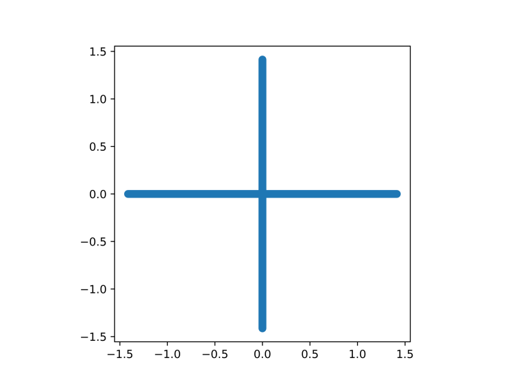
Figure 1. ${\mathsf{E}}_{2}$

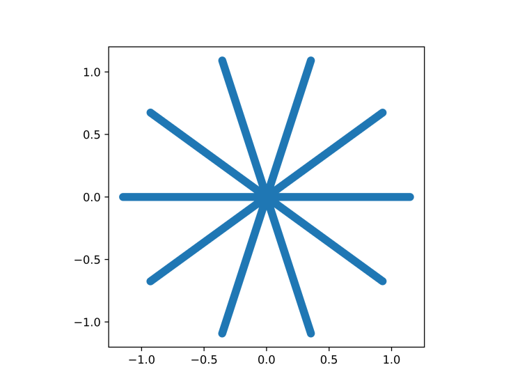
Figure 2. ${\mathsf{E}}_{5}$

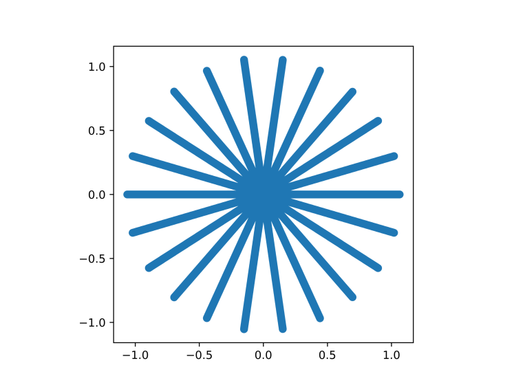
Figure 3. ${\mathsf{E}}_{11}$

Extremal polynomials of the sets ${\mathsf{E}}_{m}$ were previously studied by Peherstorfer and Steinbauer [32]. They established a connection, for $q\in[0,\infty)$, between $L^{q}$ minimal polynomials on ${\mathsf{E}}_{m}$ and specific weighted $L^{q}$ minimal polynomials on $[0,1]$, using the canonical change of variables $x=z^{m}$. In this paper, we will employ a similar change of variables, focusing on the case where $q=\infty$. This approach allows us to establish a relationship between the Chebyshev polynomials of ${\mathsf{E}}_{m}$ and weighted minimal polynomials on $[-1,1]$.

Theorem 2 handles preimages of a line segment under monomials in the complex plane. The following result gives a complete picture for such preimages of arbitrary quadratic polynomials.

Theorem 3.

Let $P(z)=z^{2}+az+b$ for $a,b\in{\mathbb{C}}$ and form ${\mathsf{E}}_{P}=\{z:P(z)\in[-2,2]\}$. Then

$${\mathcal{W}}_{2n,\infty}({\mathsf{E}}_{P})=2,\quad n\geq 1$$ (1.19)

and

$$\lim_{n\rightarrow\infty}{\mathcal{W}}_{2n+1,\infty}({\mathsf{E}}_{P})=\sqrt{2\left|c+\sqrt{c^{2}-4}\right|},$$ (1.20)

where $c=b-a^{2}/4$ and $z+\sqrt{z^{2}-4}$ maps the exterior of $[-2,2]$ to the exterior of the closed disk of radius $2$ centered at $0$. In particular, for $c\in[-2,2]$ we have

$$\lim_{n\rightarrow\infty}{\mathcal{W}}_{2n+1,\infty}({\mathsf{E}}_{P})=2.$$ (1.21)

Remark.

Note that $c\in[-2,2]$ if and only if ${\mathsf{E}}_{P}$ is connected. Hence, for ${\mathsf{E}}_{P}$ a quadratic preimage of $[-2,2]$, we have

$$\lim_{n\rightarrow\infty}{\mathcal{W}}_{n,\infty}({\mathsf{E}}_{P})=2$$

precisely when ${\mathsf{E}}_{P}$ is connected. The result in (1.20) also illustrates that we can only hope for a universal upper bound on ${\mathcal{W}}_{n,\infty}({\mathsf{E}})$ within the class of compact connected sets.

1.2. Orthogonal polynomials with respect to $\mu_{\mathsf{E}}$

The Chebyshev polynomials are the monic polynomials minimising the $L^{\infty}$ norm on a given compact set ${\mathsf{E}}\subset{\mathbb{C}}$. The same investigation on minimal polynomials can be undertaken for any $L^{p}$ norm. We shall in particular consider the sequence of monic orthogonal polynomials with respect to equilibrium measure $\mu_{\mathsf{E}}$. These are the polynomials

$$P_{n}^{\mu_{\mathsf{E}}}(z)=z^{n}+\sum_{k=0}^{n-1}c_{k}z^{k}$$

which satisfy

$$\int P_{n}^{\mu_{\mathsf{E}}}(z)\overline{\displaystyle{P_{m}^{\mu_{\mathsf{E}}}(z)}}\,d\mu_{{\mathsf{E}}}(z)=C_{n}\cdot\delta_{n,m},$$

where $C_{n}>0$ and $\delta_{n,m}$ is the Kronecker delta. It is well-known and easy to prove that all $P_{n}^{\mu_{\mathsf{E}}}$ are minimal with respect to the $L^{2}(\mu_{{\mathsf{E}}})$-norm in the sense that

$$\|P_{n}^{\mu_{\mathsf{E}}}\|_{L^{2}(\mu_{\mathsf{E}})}^{2}:=\int|P_{n}^{\mu_{\mathsf{E}}}(z)|^{2}\,d\mu_{{\mathsf{E}}}(z)=\min_{b_{0},b_{1},\ldots,b_{n-1}\in{\mathbb{C}}}\int\left|z^{n}+\sum_{k=0}^{n-1}b_{k}z^{k}\right|^{2}d\mu_{{\mathsf{E}}}(z).$$

In line with (1.4), we define the Widom factors corresponding to the $L^{2}$ minimisers on ${\mathsf{E}}$ by

$${\mathcal{W}}_{n,2}({\mathsf{E}}) :=\frac{\|\displaystyle{P_{n}^{\mu_{\mathsf{E}}}}\|_{L^{2}(\mu_{\mathsf{E}})}}{\operatorname{Cap}({\mathsf{E}})^{n}}.$$ (1.22)

The name is appropriate since Widom [54] gave a complete description of the asymptotics of ${\mathcal{W}}_{n,2}({\mathsf{E}})$ in the case where ${\mathsf{E}}$ is a finite union of Jordan curves and arcs of class $C^{2+\epsilon}$. Recent results of Alpan and Zinchenko [4] suggest a relation between the asymptotics of ${\mathcal{W}}_{n,2}({\mathsf{E}})$ and ${\mathcal{W}}_{n,\infty}({\mathsf{E}})$. In fact, the method we will use to prove Theorem 2 relies on results of Bernstein [8] where certain weighted Chebyshev polynomials are related to a class of orthogonal polynomials. This is what initially motivated our study of ${\mathcal{W}}_{n,2}({\mathsf{E}}_{m})$ and we have the following result.

Theorem 4.

With ${\mathsf{E}}_{m}$ as defined in (1.15), we have

$$\lim_{n\rightarrow\infty}{\mathcal{W}}_{n,2}({\mathsf{E}}_{m})^{2}=2.$$

Moreover, $n\mapsto{\mathcal{W}}_{2nm+l,2}({\mathsf{E}}_{m})^{2}$ is monotonically increasing for $0<{l}/{m}<1$ and monotonically decreasing for $1<{l}/{m}<2$.

Exactly the same monotonicity along subsequences was observed numerically for ${\mathcal{W}}_{n,\infty}({\mathsf{E}}_{m})$. However, without explicit formulas at hand this seems hard to prove. By relating Theorems 2 and 4, we get the following result which complements the results of [4].

Corollary 1.

The Widom factors for ${\mathsf{E}}_{m}$ satisfy that

$$\lim_{n\rightarrow\infty}{\mathcal{W}}_{n,2}({\mathsf{E}}_{m})^{2}=\lim_{n\rightarrow\infty}{\mathcal{W}}_{n,\infty}({\mathsf{E}}_{m}).$$ (1.23)

Based on the results of [4], it was conjectured in [18] that if ${\mathsf{E}}$ is a smooth Jordan arc, then

$$\lim_{n\rightarrow\infty}{\mathcal{W}}_{n,2}({\mathsf{E}})^{2}=\lim_{n\rightarrow\infty}{\mathcal{W}}_{n,\infty}({\mathsf{E}}).$$ (1.24)

It is known that (1.24) holds for straight line segments and circular arcs as in (1.13), see [18] and [4]. In our case we are not dealing with a single Jordan arc but rather a union of Jordan arcs. Nevertheless, our approach may still shed new light on the above conjecture.

1.3. Outline

This article is organised as follows. In Section 2 we discuss the $S$-property and the Chebotarev problem, and use these concepts to present a proof of Theorem 1. In Section 3 we consider Chebyshev polynomials on quadratic preimages of $[-2,2]$ and illustrate how Bernstein’s method for determining the asymptotic behaviour of weighted Chebyshev polynomials on an interval (summarised in the appendix) can be applied to solve problems in the complex plane. We specifically establish Theorem 2 for $m=2$ and extend this result to Theorem 3, which completely describes the asymptotic behavior of the Widom factors for quadratic preimages of $[-2,2]$. The findings for ${\mathsf{E}}_{2}$ are extended to the setting of all ${\mathsf{E}}_{m}$ sets in Section 4, demonstrating the alternation properties of Chebyshev polynomials in this context and providing a complete proof of Theorem 2.

In Section 5 we consider polynomials orthogonal with respect to equilibrium measure of ${\mathsf{E}}_{m}$ and prove Theorem 4, that the associated Widom factors converge to $2$. We also show that the numerically observed monotonic behavior of the corresponding Chebyshev norms holds for the orthogonal polynomials in this setting. Additional insight into this monotonicity is presented in Section 6, drawing upon conformal mappings and geometric considerations. Ultimately, we address potential future research directions in Section 7. With Conjecture 1, we propose a potential connection between Shabat polynomial preimages and the convergence of Widom factors to $2$. This conjecture finds support in numerical simulations. We hold the view that a fundamental prerequisite for sets to exhibit such Widom factors lies in the geometric $S$-property.

2. The $S$-property and Chebotarev sets

We now direct our focus towards compact sets ${\mathsf{E}}\subset{\mathbb{C}}$ exhibiting a certain symmetry property which turns out to be of importance regarding the convergence behaviour $\lim_{n\rightarrow\infty}{\mathcal{W}}_{n}({\mathsf{E}})=2$. In fact, this is exactly what we will use to prove Theorem 1.

The symmetry property in question is called the $S$-property and was introduced by Stahl in the 1980s to study certain extremal domains in the complex plane. The “$S$” in the name is therefore ambiguous; it can be read as symmetry but also as Stahl. We will present a simplified version of the $S$-property, adapted to our needs, following [45, Definition 2]. For a more comprehensive exploration of its connection to extremal domains of meromorphic functions, we direct the reader to [43, 44, 46].

Definition 1.

Let ${\mathsf{E}}\subset{\mathbb{C}}$ be a compact set with $\operatorname{Cap}({\mathsf{E}})>0$ and suppose ${\mathbb{C}}\setminus{\mathsf{E}}$ is connected. Assume further that there exists a subset ${\mathsf{E}}_{0}\subset{\mathsf{E}}$ with $\operatorname{Cap}({\mathsf{E}}_{0})=0$ such that

$${\mathsf{E}}\setminus{\mathsf{E}}_{0}=\bigcup_{i\in I}\gamma_{i}$$

where the $\gamma_{i}$’s are disjoint open analytic Jordan arcs and $I\subset{\mathbb{N}}$. Then ${\mathsf{E}}$ is said to satify the $S$-property if

$$\frac{\partial G_{\mathsf{E}}}{\partial n_{+}}(z)=\frac{\partial G_{\mathsf{E}}}{\partial n_{-}}(z)$$ (2.1)

holds for all $z\in{\mathsf{E}}\setminus{\mathsf{E}}_{0}$, where $n_{+}$ and $n_{-}$ denote the unit normals from each side of the arcs.

Remark.

The assumption of the arcs $\gamma_{i}$ being analytic is redundant, as mild smoothness conditions coupled with the fulfillment of (2.1) imply the analyticity of these arcs. This observation is mentioned in [45] without providing a formal proof.

The initial question to address in the context of reducing the smoothness of individual arcs pertains to the existence of the normal derivatives in (2.1). The proof of [53, Proposition 2.2] invokes the Kellogg–Warschawski theorem [34, Theorem 3.6] to establish that if the coordinates of the arcs are differentiable and their derivatives are Hölder continuous, then the normal derivatives of $G_{\mathsf{E}}$ exist along each $\gamma_{i}$. Consequently, it is reasonable to discuss the fulfillment of (2.1) for arcs belonging to the class $C^{2+\epsilon}$. In [3, Theorem 1.4], it is established that with this smoothness assumption, the arcs $\gamma_{i}$ indeed become analytic when (2.1) is satisfied.

The concept of Chebotarev sets is closely related to the $S$-property. These sets are characterized by having minimal capacity while being constrained to include a specific collection of points. To elaborate, the Chebotarev problem, originally posed as a question to Pólya [33], revolves around the quest for the following set:

Definition 2.

Given a finite number of points $\alpha_{1},\ldots,\alpha_{m}\in{\mathbb{C}}$, the compact connected set ${\mathsf{E}}$ that contains these points and has minimal logarithmic capacity among all such sets is called the Chebotarev set of $\alpha_{1},\ldots,\alpha_{m}$. It is denoted by ${\mathsf{E}}(\alpha_{1},\dotsc,\alpha_{m})$.

That such sets exist and are unique was proven by Grötzsch [24]. He also characterised the Chebotarev sets in terms of the behaviour of certain quadratic differentials. Stahl [46, Theorem 11] proved that any solution to a Chebotarev problem must satisfy the $S$-property. In fact, he gave both necessary and sufficient conditions for a set to be a Chebotarev set in terms of the $S$-property and additional geometric conditions. For further properties of Chebotarev sets, see, e.g., [28, Chapter 1]. The case of $m=3$ is studied in detail in this monograph.

Interestingly, there is also a relation between Chebotarev sets and polynomial preimages of intervals. Schiefermayr [39] proved that if $P$ is a polynomial and $P^{-1}([-1,1])$ is connected, then this preimage is the solution to a Chebotarev problem. More specifically, if $\alpha_{1},\ldots,\alpha_{m}$ is an enumeration of the distinct simple zeros of $P^{2}-1$ then

$$P^{-1}([-1,1])={\mathsf{E}}(\alpha_{1},\dotsc,\alpha_{m}).$$

In particular, any such polynomial preimage satisfies the $S$-property.

By combining Stahl’s results on minimal capacity with recent results of Alpan, we can easily prove that equality is possible in (1.14) only for straight line segments. In this case, as we know, ${\mathcal{W}}_{n,\infty}({\mathsf{E}})=2$ for every $n$.

Proof of Theorem 1.

Let ${\mathsf{E}}$ be a Jordan arc of class $C^{2+\epsilon}$, connecting two complex points $a$ and $b$. The fact that

$$\limsup_{n\rightarrow\infty}{\mathcal{W}}_{n,\infty}({\mathsf{E}})\leq 2$$

is precisely the content of [3, Theorem 1.2]. For equality to hold, it must be so that (2.1) holds at all interior points of the arc. As explained in the remark following Definition 1, this implies that ${\mathsf{E}}$ is an analytic Jordan arc possessing the $S$-property. By [46, Theorem 11], ${\mathsf{E}}$ is therefore the solution to the Chebotarev problem corresponding to the points $a$ and $b$. Hence ${\mathsf{E}}(a,b)=[a,b]$, where $[a,b]$ denotes the straight line segment in ${\mathbb{C}}$ between $a$ and $b$ (see, e.g., [28]). This completes the proof. ∎

In the remainder of this article, we will consider polynomial preimages of $[-2,2]$. All the sets to be considered have in common that they satisfy the $S$-property and hence are minimal sets for a Chebotarev problem.

3. Quadratic preimages

The general framework is sets of the form

$${\mathsf{E}}_{m}:=\bigl{\{}z:z^{m}\in[-2,2]\bigr{\}}.$$

These are star-shaped connected sets which are invariant under rotations by $\pi/m$ radians, see Figures 3–3. Furthermore, [39, Theorem 2] implies that ${\mathsf{E}}_{m}$ is the Chebotarev set corresponding to the collection of points

$$\bigl{\{}2^{1/m}e^{i\pi k/m}:k=1,\dotsc,2m\bigr{\}}.$$

To begin with, we consider the case where $m=2$ even though our results are true for any $m\in{\mathbb{N}}$. The motivation for this is that we more transparently can provide an intuition for the problem when $m=2$. We end the section by also considering the setting of a general quadratic preimage.

Consider the set

$${\mathsf{E}}_{2}=\bigl{\{}z:z^{2}\in[-2,2]\bigr{\}}=\bigl{[}-\sqrt{2},\sqrt{2}\,\bigr{]}\cup i\bigl{[}-\sqrt{2},\sqrt{2}\,\bigr{]},$$

which has the shape of a “plus sign”. Equation (1.7) implies that the Green’s function for $\overline{{\mathbb{C}}}\setminus{\mathsf{E}}_{2}$ with pole at $\infty$ is given by

$$G_{{\mathsf{E}}_{2}}(z)=\frac{G_{[-2,2]}(z^{2})}{2}=\log|z|+o(1),\quad z\rightarrow\infty.$$

From this we also see that $\operatorname{Cap}({\mathsf{E}}_{2})=1$ and hence

$${\mathcal{W}}_{n,\infty}({\mathsf{E}}_{2})=\|T_{n}^{{\mathsf{E}}_{2}}\|_{{\mathsf{E}}_{2}}.$$

Recall now that a lemma from [27] states that if ${\mathsf{E}}$ is an infinite compact set and $P$ a polynomial of degree $m$ with leading coefficient $a_{m}$, then

$$T_{nm}^{P^{-1}({\mathsf{E}})}=(T_{n}^{{\mathsf{E}}}\circ P)/{a_{m}^{n}}.$$ (3.1)

For a recent proof, see [16]. In our setting this immediately implies that

$$T_{2n}^{{\mathsf{E}}_{2}}(z)=T_{n}^{[-2,2]}(z^{2}),$$

as was also proven in [32]. Therefore, all the Chebyshev polynomials of even degree for ${\mathsf{E}}_{2}$ can be determined explicitly. This further implies that we can calculate “half” of the norms, that is,

$${\mathcal{W}}_{2n}({\mathsf{E}}_{2})=\|T_{2n}^{{\mathsf{E}}_{2}}\|_{{\mathsf{E}}_{2}}=\|T_{n}^{[-2,2]}\|_{[-2,2]}=2.$$

What is left to determine are the Chebyshev polynomials of odd degree for ${\mathsf{E}}_{2}$. The set ${\mathsf{E}}_{2}$ is symmetric since it is invariant under rotations by $\pi/2$ radians. More precisely,

$$i{\mathsf{E}}_{2}=\{iz:z\in{\mathsf{E}}_{2}\}={\mathsf{E}}_{2},$$

and by uniqueness of the Chebyshev polynomials it thus follows that

$$(-i)^{n}T_{n}^{{\mathsf{E}}_{2}}(iz)=T_{n}^{{\mathsf{E}}_{2}}(z).$$

From this relation we get certain conditions on the coefficients of $T_{2n+1}^{{\mathsf{E}}_{2}}$. Several of them will vanish and considering degrees of the form $4n+l$ with $l\in\{1,3\}$, we have

$$\begin{split}T_{4n+l}^{{\mathsf{E}}_{2}}(z)&=z^{4n+l}+\sum_{k=0}^{n-1}a_{k}z^{4k+l},\quad a_{k}\in\mathbb{R}.\end{split}$$ (3.2)

In particular, $T_{4n+l}^{{\mathsf{E}}_{2}}$ has a zero at the origin of order at least $l$. However, as we shall see below, this is the precise order of the zero.

Before stating our main characterisation of $T_{4n+l}^{{\mathsf{E}}_{2}}$, we recall that an alternating set for a function $f:I\rightarrow\mathbb{C}$ is an ordered sequence of points $\{x_{k}\}\subset I$ such that

$$f(x_{k})=\sigma(-1)^{k}\|f\|_{I},\quad|\sigma|=1.$$

Lemma 1.

For $l\in\{1,3\}$, the Chebyshev polynomial $T_{4n+l}^{{\mathsf{E}}_{2}}$ is characterised by alternation in the following way:

• $T_{4n+l}^{{\mathsf{E}}_{2}}$ has alternating sets consisting of $n+1$ points on each of the sets $i^{k}[0,\sqrt{2}]$, $k=0,1,2,3.$

• $T_{4n+l}^{{\mathsf{E}}_{2}}$ can be represented as in (3.2).

Proof.

We have already motivated why (3.2) should hold for $T_{4n+l}^{{\mathsf{E}}_{2}}$. This also implies that $T_{4n+l}^{{\mathsf{E}}_{2}}$ is purely real on the real axis and purely imaginary on the imaginary axis. Now, basic theory for Chebyshev polynomials implies that $T_{4n+l}^{{\mathsf{E}}_{2}}$ has at least $4n+l+1$ extremal points (see, e.g., [30, Lemma 2.5.3]). Due to symmetry, there are at least $n+1$ extremal points on each of the rays

$$i^{k}[0,\sqrt{2}],\quad k=0,1,2,3.$$

It is enough to consider alternation on one of these rays since, by symmetry, the situation is entirely analogous on each of the rays. We therefore fix our attention to $[0,\sqrt{2}]$ where $T_{4n+l}^{{\mathsf{E}}_{2}}$ is real valued. If there were two adjacent extremal points on $[0,\sqrt{2}]$ with the same sign, then this would imply that the derivative $(T_{4n+l}^{{\mathsf{E}}_{2}})^{\prime}$ should have at least $4\left(n+1\right)\geq 4n+l+1$ zeros. But this is a contradiction since the degree of the derivative is $4n+l-1$.

To prove the other direction, we apply the intermediate value theorem in the following way. Suppose $Q$ is a polynomial which can be represented as in (3.2). Then $Q$ will be real-valued on the real line and imaginary-valued on the imaginary axis. Assume further that $Q$ possesses alternating sets as in the statement of the lemma. If $Q\neq T_{4n+l}^{{\mathsf{E}}_{2}}$, then

$$\|Q\|_{{\mathsf{E}}_{2}}>\|T_{4n+l}^{{\mathsf{E}}_{2}}\|_{{\mathsf{E}}_{2}}$$

and it follows from the intermediate value theorem that $Q-T_{4n+l}^{{\mathsf{E}}_{2}}$ must have a zero between any two consecutive points in the alternating sets for $Q$. But this amounts to at least $4n+l$ zeros in addition to the zero of multiplicity $l$ at $0$. Hence the number of zeros would be greater than the degree of $Q-T_{4n+l}^{{\mathsf{E}}_{2}}$ which is impossible. Therefore, we conclude that $Q=T_{4n+l}^{{\mathsf{E}}_{2}}$. ∎

One implication of this lemma is the fact that all the zeros of $T_{2n+1}^{{\mathsf{E}}_{2}}$ are simple, except the one at $z=0$ for $T_{4n+3}^{{\mathsf{E}}_{2}}$. A further implication is that we can determine the first few Chebyshev polynomials for ${\mathsf{E}}_{2}$ explicitly:

$$T_{1}^{{\mathsf{E}}_{2}}(z) =z,$$

$$T_{3}^{{\mathsf{E}}_{2}}(z) =z^{3},$$

$$T_{5}^{{\mathsf{E}}_{2}}(z) =z^{5}-\frac{5\left(3-\frac{15^{2/3}}{\sqrt[3]{9+4\sqrt{6}}}+\sqrt[3]{15(9+4\sqrt{6})}\right)^{4}}{5184}z.$$

Since already the expression for $T_{5}^{{\mathsf{E}}_{2}}$ gets rather complicated, there seems to be no simple closed form for $T_{2n+1}^{{\mathsf{E}}_{2}}$ when $n$ is large.

Lemma 1 also implies that the image of ${\mathsf{E}}_{2}$ under $T_{2n+1}^{{\mathsf{E}}_{2}}$ is again a plus-shaped set, namely

$$T_{4n+l}^{{\mathsf{E}}_{2}}({\mathsf{E}}_{2})=\bigcup_{k=0}^{3}i^{k}\bigl{[}0,\|T_{4n+l}^{{\mathsf{E}}_{2}}\|_{{\mathsf{E}}_{2}}\bigr{]}=\frac{\|T_{4n+l}^{{\mathsf{E}}_{2}}\|_{{\mathsf{E}}_{2}}}{\sqrt{2}}{\mathsf{E}}_{2}.$$

To further understand the behaviour of $\|T_{4n+l}^{{\mathsf{E}}_{2}}\|_{{\mathsf{E}}_{2}}$, we introduce the preimage

$${\mathsf{E}}_{2}^{n,l}:=(T_{4n+l}^{{\mathsf{E}}_{2}})^{-1}\bigl{(}T_{4n+l}^{{\mathsf{E}}_{2}}({\mathsf{E}}_{2})\bigr{)}=(T_{4n+l}^{{\mathsf{E}}_{2}})^{-1}\left(\bigcup_{k=0}^{3}i^{k}\bigl{[}0,\|T_{4n+l}^{{\mathsf{E}}_{2}}\|_{{\mathsf{E}}_{2}}\bigr{]}\right)$$ (3.3)

which clearly contains ${\mathsf{E}}_{2}$ as a subset. Due to the alternating property described in Lemma 1, we deduce that ${\mathsf{E}}_{2}^{n,l}$ is connected and a finite union of Jordan arcs. These in turn intersect at the zeros of $T_{4n+l}^{{\mathsf{E}}_{2}}$. Moreover, ${\mathsf{E}}_{2}^{n,l}$ is nothing but the Chebotarev set corresponding to the points

$$(T_{4n+l}^{{\mathsf{E}}_{2}})^{-1}\Bigl{(}\bigl{\{}i^{k}\|T_{4n+l}^{{\mathsf{E}}_{2}}\|_{{\mathsf{E}}_{2}}:k=0,1,2,3\bigr{\}}\Bigr{)}.$$

Applying (1.7) and using the fact that $\operatorname{Cap}(\alpha{\mathsf{E}})=|\alpha|\operatorname{Cap}({\mathsf{E}})$ for any $\alpha\in{\mathbb{C}}$, we see that

$$\operatorname{Cap}({\mathsf{E}}_{2}^{n,l})=\operatorname{Cap}\left(\frac{\|T_{4n+l}^{{\mathsf{E}}_{2}}\|_{{\mathsf{E}}_{2}}}{\sqrt{2}}{\mathsf{E}}_{2}\right)^{1/{4n+l}}=\left(\frac{\|T_{4n+l}^{{\mathsf{E}}_{2}}\|_{{\mathsf{E}}_{2}}}{\sqrt{2}}\right)^{1/{4n+l}}.$$ (3.4)

Rearranging this equality leads to the identity

$$\|T_{4n+l}^{{\mathsf{E}}_{2}}\|_{{\mathsf{E}}_{2}}=\sqrt{2}\operatorname{Cap}({\mathsf{E}}_{2}^{n,l})^{4n+l}.$$ (3.5)

Since ${\mathsf{E}}_{2}^{n,l}\supset{\mathsf{E}}_{2}$, we have $\operatorname{Cap}({\mathsf{E}}_{2}^{n,l})\geq\operatorname{Cap}({\mathsf{E}}_{2})=1$ and conclude that

$$\|T_{4n+l}^{{\mathsf{E}}_{2}}\|_{{\mathsf{E}}_{2}}\geq\sqrt{2}.$$ (3.6)

Note that the reasoning outlined above follows the same method of proof that we employed to prove the lower bounds of Szegő and Schiefermayr in the introduction. However, the conclusion is not equally strong. The lower bound in (3.6) is saturated for $T_{1}^{{\mathsf{E}}_{2}}$, but otherwise not. Using $zT_{2n}^{{\mathsf{E}}_{2}}(z)$ as a trial polynomial, we find that

$$\|T_{2n+1}^{{\mathsf{E}}_{2}}\|_{{\mathsf{E}}_{2}}\leq\|zT_{2n}^{{\mathsf{E}}_{2}}\|_{{\mathsf{E}}_{2}}\leq\sqrt{2}\|T_{2n}^{{\mathsf{E}}_{2}}\|_{{\mathsf{E}}_{2}}=2^{3/2}.$$

This upper bound is only saturated by $T_{3}^{{\mathsf{E}}_{2}}$. To close the gap between $\sqrt{2}$ and $2^{3/2}$ in the limit as $n\to\infty$, additional insight is needed. We shall settle this issue in the next subsection.

At this point, we would like to highlight an intriguing observation that, to date, remains open. Recall that the Remez algorithm [36, 37] uses the theory of alternation to numerically compute Chebyshev polynomials of real compact sets. This algorithm was generalised to the complex setting by Tang [49] and further refined by Modersitzki and Fischer [22]. Using an implementation of this generalised algorithm, we can compute the norms of the Chebyshev polynomials for degree up to at least $60$. What materialised for ${\mathsf{E}}_{2}$ is illustrated in Figure 4.

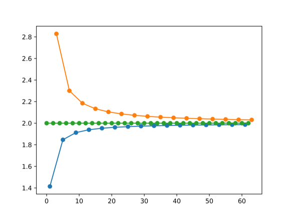
Figure 4. The norm of $T_{n}^{{\mathsf{E}}_{2}}$ plotted as a function of the degree $n$. The three natural subsequences are highlighted in different colors.

As we already know, $\|T_{n}^{{\mathsf{E}}_{2}}\|_{{\mathsf{E}}_{2}}=2$ for all even $n$. For odd $n$, there are two natural subsequences counting modulo $4$. It appears that $n\mapsto\|T_{4n+1}^{{\mathsf{E}}_{2}}\|_{{\mathsf{E}}_{2}}$ is monotonically increasing, while $n\mapsto\|T_{4n+3}^{{\mathsf{E}}_{2}}\|_{{\mathsf{E}}_{2}}$ appears to be monotonically decreasing. Similar patterns emerge for the general ${\mathsf{E}}_{m}$ sets.

3.1. A related weighted problem and the proof of Theorem 2 for $m=2$

Rather than employing (3.5) and attempting to directly estimate the capacity of ${\mathsf{E}}_{2}^{n,l}$, we shall shift the minimax problem to a weighted problem on ${\mathbb{R}}$ which can, in turn, be solved using a method of Bernstein [8].

Based on (3.2), the Chebyshev polynomials of odd degree for ${\mathsf{E}}_{2}$ can be represented as

$$T_{4n+l}^{{\mathsf{E}}_{2}}(z)=z^{4n+l}+\sum_{k=0}^{n-1}a_{k}z^{4k+l}=z^{l}\left(z^{4n}+\sum_{k=0}^{n-1}a_{k}z^{4k}\right)=z^{l}Q_{n,l}(z^{4}),$$

where $Q_{n,l}$ is a real monic polynomial of degree $n$. Note that $Q_{n,l}$ has the property that it minimises

$$\max_{z\in{\mathsf{E}}_{2}}|z^{l}|\bigl{|}Q_{n,l}(z^{4})\bigr{|}$$

among all monic polynomials of degree $n$. Since $|z^{1/4}|$ is single-valued, we can change the variables via the transformation $x=z^{4}/2-1$ and obtain that $Q_{n,l}$ minimises

$$\max_{x\in[-1,1]}2^{l/4}(x+1)^{{l}/{4}}\left|Q_{n,l}\bigl{(}2(x+1)\bigr{)}\right|.$$

Put differently, and noting that $2^{-n}Q_{n,l}(2(x+1))$ is monic, we see that

$$\|T_{4n+l}^{{\mathsf{E}}_{2}}\|_{{\mathsf{E}}_{2}}=2^{n+{l}/{4}}\min_{b_{0},b_{1},\ldots,b_{n-1}\in{\mathbb{R}}}\max_{x\in[-1,1]}(x+1)^{{l}/{4}}\left|x^{n}+\sum_{k=0}^{n-1}b_{k}x^{k}\right|.$$ (3.7)

In the case of $l=0$, we are back at the classical problem solved by Chebyshev and the polynomials $T_{n}$ of (1.1). For $l=2$, the solution is given by the so-called Chebyshev polynomials of the third kind, denoted $V_{n}$. This is easily seen by noting that

$$(x+1)^{1/2}V_{n}(x)=\sqrt{2}\cos\bigl{(}(n+1/2)\arccos(x)\bigr{)}$$

oscillates on $[-1,1]$ between precisely $n+1$ extrema of equal magnitude. However, we are interested in the cases $l=1,3$ where no such simple formulas seem to be available.

The key is to recall that $T_{n}$ and $V_{n}$ are also orthogonal polynomials. Both are special cases of the Jacobi polynomials $P_{n}^{(\alpha,\beta)}$ which have been studied in detail and are orthogonal with respect to $(1-x)^{\alpha}(1+x)^{\beta}$ on $[-1,1]$. If we have a non-negative weight function $w$ defined on $[-1,1]$, we will use the notation ${T_{n}^{w}}$ to represent the minimiser of

$$\max_{x\in[-1,1]}w(x)|P_{n}(x)|,$$

where $P_{n}$ ranges over all monic polynomials of degree $n$. This minimizer is uniquely defined for sufficiently large $n$ under the conditions that $w$ does not vanish at infinitely many points and $wP$ is bounded for some polynomial $P$. A naive comparison of the $L^{\infty}$ and $L^{2}$ norms suggests that ${T_{n}^{w}}$ could be related to the monic orthogonal polynomials with respect to $w(x)^{2}/\sqrt{1-x^{2}}$ on $[-1,1]$. In our setting, the weight is given by

$$w_{l}(x)=(x+1)^{l/4}$$

and we thus search for a relation between ${T_{n}^{w_{l}}}$ and $P_{n}^{(-1/2,\,\beta_{l})}$ for $\beta_{l}=(l-1)/2$. In special cases (such as $l=0,2$) we have an exact match and the polynomials coincide. But even for general $l$, there are striking similarities between the polynomials. In [8], Bernstein proved that $w_{l}P_{n}^{(-1/2,\,\beta_{l})}$ is asymptotically alternating on $[-1,1]$ as $n\to\infty$ and because of that, $P_{n}^{(-1/2,\,\beta_{l})}$ are excellent trial polynomials when studying the limit of $\|w_{l}T_{n}^{w_{l}}\|_{[-1,1]}$.

We shall formulate Bernstein’s full result below. As the proof is only available in French or Russian, we decided to include a detailed review of this method in the appendix. While our presentation primarily adheres to Bernstein’s original proof, we are able to streamline some arguments by integrating findings from Achieser and Chebyshev alongside Bernstein’s work.

Theorem 5 (Bernstein [8]).

Suppose $\alpha_{k}\in\mathbb{R}$ and $b_{k}\in[-1,1]$ for $k=0,1,\ldots,m$. Consider a weight function $w:[-1,1]\rightarrow[0,\infty)$ of the form

$$w(x)=w_{0}(x)\prod_{k=0}^{m}|x-b_{k}|^{\alpha_{k}},$$ (3.8)

where $w_{0}$ is Riemann integrable and satisfies $1/M\leq w_{0}(x)\leq M$ for some constant $M\geq 1$. Then

$$\|wT_{n}^{w}\|_{[-1,1]}=2^{1-n}\exp\left\{\frac{1}{\pi}\int_{-1}^{1}\frac{\log w(x)}{\sqrt{1-x^{2}}}dx\right\}\bigl{(}1+o(1)\bigr{)}$$ (3.9)

as $n\rightarrow\infty$.

With Bernstein’s theorem at hand, we can now prove Theorem 2. We isolate the following lemma since it will be used multiple times in the rest of the article.

Lemma 2.

For any $z\in{\mathbb{C}}$, we have

$$\frac{1}{\pi}\int_{-1}^{1}\frac{\log|x-z|}{\sqrt{1-x^{2}}}dx=\log\frac{\left|z+\sqrt{z^{2}-1}\right|}{2},$$ (3.10)

where $z+\sqrt{z^{2}-1}$ maps ${\mathbb{C}}\setminus[-1,1]$ conformally onto ${\mathbb{C}}\setminus\overline{{\mathbb{D}}}$. In particular, for $z\in[-1,1]$ the integral is constantly equal to $-\log 2$.

Proof.

Recall that the Green’s function for $\overline{{\mathbb{C}}}\setminus[-1,1]$ with pole at $\infty$ is given by

$$G_{[-1,1]}(z)=\log\left|z+\sqrt{z^{2}-1}\right|.$$

Since the integral on the left-hand side of (3.10) is nothing but the potential for the equilibrium measure of $[-1,1]$, we conclude that

$$\frac{1}{\pi}\int_{-1}^{1}\frac{\log|x-z|}{\sqrt{1-x^{2}}}dx=G_{[-1,1]}(z)+\log\operatorname{Cap}\bigl{(}[-1,1]\bigr{)}=\log\frac{\left|z+\sqrt{z^{2}-1}\right|}{2}$$

for $z\notin[-1,1]$. If instead $z\in[-1,1]$, we find by continuity of $G_{[-1,1]}$ on ${\mathbb{C}}$ and monotone convergence that

$$\frac{1}{\pi}\int_{-1}^{1}\frac{\log|x-z|}{\sqrt{1-x^{2}}}dx =\lim_{\epsilon\downarrow 0}\frac{1}{\pi}\int_{-1}^{1}\frac{\log|x-(z+i\epsilon)|}{\sqrt{1-x^{2}}}dx$$

$$=\lim_{\epsilon\downarrow 0}\log\frac{\left|(z+i\epsilon)+\sqrt{(z+i\epsilon)^{2}-1}\right|}{2}=\log\frac{\left|z+\sqrt{z^{2}-1}\right|}{2}=-\log 2.$$

This completes the proof. ∎

We are now in position to prove the limiting result for ${\mathsf{E}}_{2}$. As we shall see in Section 4, the method of proof actually handles all cases in Theorem 2.

Proof of Theorem 2 for $m=2$.

Let $w_{l}(x)=(x+1)^{{l}/{4}}$ with $l=1,3$. Theorem 5 implies that

$$\|T_{n}^{w_{l}}w_{l}\|_{[-1,1]}=2^{1-n}\exp\left\{\frac{l}{4\pi}\int_{-1}^{1}\frac{\log(x+1)}{\sqrt{1-x^{2}}}dx\right\}\bigl{(}1+o(1)\bigr{)}$$

as $n\rightarrow\infty$. Applying Lemma 2 gives us that the the exponential on the right-hand side reduces to

$$\exp\left\{\frac{l}{4}\cdot\log\frac{1}{2}\right\}=2^{-{l}/{4}}.$$

By (3.7), we therefore find that

$$\|T_{4n+l}^{{\mathsf{E}}_{2}}\|_{{\mathsf{E}}_{2}}=2^{n+{l}/{4}}\|T_{n}^{w_{l}}w_{l}\|_{[-1,1]}=2\bigl{(}1+o(1)\bigr{)},$$

which settles the claim for ${\mathsf{E}}_{2}$. ∎

3.2. General quadratic preimages

We proceed by considering general quadratic preimages of $[-2,2]$ and show that our method can be applied to this case as well. Of course, such preimages need not be connected and we should not expect the Widom factors to always converge to $2$. As in Theorem 3, we shall consider sets of the form

$${\mathsf{E}}_{P}=\bigl{\{}z:P(z)\in[-2,2]\bigr{\}},$$ (3.11)

where $P(z)=z^{2}+az+b$ and $a,b\in\mathbb{C}$. Now, let us present a proof of this result.

Proof of Theorem 3.

By (1.7), we have $\operatorname{Cap}({\mathsf{E}}_{P})=1$ and thus

$${\mathcal{W}}_{n,\infty}({\mathsf{E}}_{P})=\|T_{n}^{{\mathsf{E}}_{P}}\|_{{\mathsf{E}}_{P}}.$$

The first part of the theorem (i.e., (1.19) for even degree) is easily handled by (3.1). In order to prove (1.20), we note that

$$z^{2}+az+b=\left(z+\frac{a}{2}\right)^{2}+c,\quad c=b-a^{2}/4.$$

Therefore, it suffices to consider the case of

$${\mathsf{E}}_{P_{c}}=\bigl{\{}z:z^{2}+c\in[-2,2]\bigr{\}}.$$

As $z\in{\mathsf{E}}_{P_{c}}$ if and only if $-z\in{\mathsf{E}}_{P_{c}}$, we deduce that

$$T_{2n+1}^{{\mathsf{E}}_{P_{c}}}(z)=z^{2n+1}+\sum_{k=0}^{n-1}a_{k}z^{2k+1},\quad a_{k}\in{\mathbb{C}}.$$

Hence, since $|\sqrt{z}|=|z|^{1/2}$ is single-valued, we can apply the change of variables $x=(z^{2}+c)/2$ leading to

$$\|T_{2n+1}^{{\mathsf{E}}_{P_{c}}}\|_{{\mathsf{E}}_{P_{c}}}=2^{n+{1}/{2}}\min_{b_{0},b_{1},\ldots,b_{n-1}\in\mathbb{R}}\max_{x\in[-1,1]}\sqrt{|x-c/2|}\left|x^{n}+\sum_{k=0}^{n-1}b_{k}x^{k}\right|.$$

Since the weight function $\sqrt{|x-c/2|}$ is of the form (3.8) — in fact, we only need $w_{0}$ for $c\notin[-2,2]$ — Theorem 5 implies that

$$\|T_{2n+1}^{{\mathsf{E}}_{P_{c}}}\|_{{\mathsf{E}}_{P_{c}}}=2^{3/2}\exp\left\{\frac{1}{2\pi}\int_{-1}^{1}\frac{\log|x-c/2|}{\sqrt{1-x^{2}}}dx\right\}\bigl{(}1+o(1)\bigr{)}$$ (3.12)

as $n\rightarrow\infty$. Using Lemma 2 to rewrite the exponential term, we conclude that

$$\lim_{n\to\infty}\|T_{2n+1}^{{\mathsf{E}}_{P_{c}}}\|_{{\mathsf{E}}_{P_{c}}}=2^{3/2}\cdot\sqrt{\frac{\bigl{|}{c}/{2}+\sqrt{\left({c}/{2}\right)^{2}-1}\bigr{|}}{2}}=\sqrt{2\left|c+\sqrt{c^{2}-4}\right|}$$

and the proof is complete. ∎

Remark.

As the attentive reader may have noticed, we employ a different change of variables in the proof of Theorem 3 compared to what is used for ${\mathsf{E}}_{2}$. This is because we no longer have the same degree of symmetry at our disposal. In principle, one could have applied the change of variables $x=z^{2}/2$ for ${\mathsf{E}}_{2}$ as well. However, it seems more appropriate to leverage all the available structure, especially considering the distinct behavior of $\|T_{4n+l}^{{\mathsf{E}}_{2}}\|_{{\mathsf{E}}_{2}}$ for $l=1,3$.

As pointed out in the introduction, ${\mathsf{E}}_{P}$ is only connected when $c\in[-2,2]$. For otherwise the critical value of $z^{2}+c$ lies outside $[-2,2]$. The corresponding sets have the shape of a “stretched plus” and we appear to loose the monotonicity of

$$n\mapsto\|T_{4n+l}^{{\mathsf{E}}_{P}}\|_{{\mathsf{E}}_{P}},\quad l=1,3$$

whenever $c\neq 0$, see Figures 6–6.

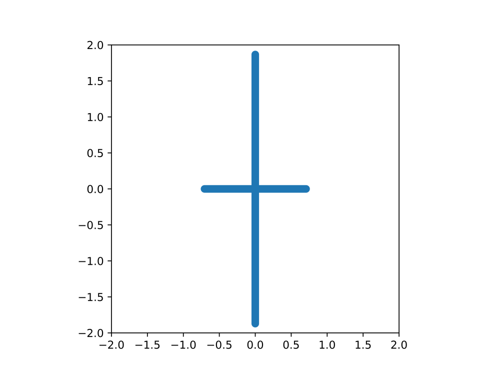
Figure 5. ${\mathsf{E}}_{P_{c}}$ for $c=-3/2$

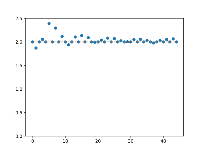
Figure 6. The norms of $T_{n}^{{\mathsf{E}}_{P}}$ for $c=-3/2$

For $c\in{\mathbb{R}}\setminus[-2,2]$, the set ${\mathsf{E}}_{P}$ is either purely real or purely imaginary and consists of two disjoint intervals of the same length. This case is well-understood and the fact that $n\mapsto{\mathcal{W}}_{n,\infty}({\mathsf{E}}_{P})$ is asymptotically periodic goes back to Achieser [1]. Remarkably, this pattern persists for all non-real values of $c$ where ${\mathsf{E}}_{P}$ comprises two disjoint analytic Jordan arcs of opposite sign. See Figures 8–8 for such an example including the corresponding norms.

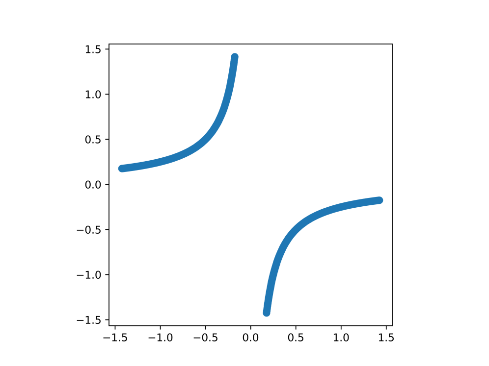
Figure 7. ${\mathsf{E}}_{P_{c}}$ for $c=i/2$

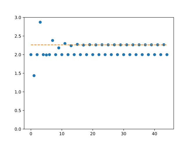
Figure 8. The norms of $T_{n}^{{\mathsf{E}}_{P}}$ for $c=i/2$

4. General $m$-stars

The aim of this section is to generalise the content of Section 3 to the general setting of $m\geq 2$ and in particular prove Theorem 2. As the strategy is very similar, we shall not provide all details in the proof. Let us first state the alternation result that still holds in this setting.

Lemma 3.

For $n,l\in\mathbb{N}$ and $0\leq l<2m$, the polynomial $T_{2nm+l}^{{\mathsf{E}}_{m}}$ is characterised by the following two properties:

• for $x\in[0,2^{1/m}]$ and $k=0,1,\ldots,2m-1$, the polynomial $T_{2nm+l}^{{\mathsf{E}}_{m}}(e^{i\pi k/m}x)$ has an alternating set consisting of $n+1$ points,

• $T_{2nm+l}^{{\mathsf{E}}_{m}}$ is of the form

  $$T_{2nm+l}^{{\mathsf{E}}_{m}}(z)=z^{2nm+l}+\sum_{k=0}^{n-1}a_{2km+l}z^{2km+l},\quad a_{2km+l}\in{\mathbb{R}}.$$ (4.1)

Proof.

We first show that $T_{2nm+l}^{{\mathsf{E}}_{m}}$ can be represented as in (4.1). Since $z\in{\mathsf{E}}_{m}$ if and only if $e^{i\pi/m}z\in{\mathsf{E}}_{m}$, we find that

$$T_{2nm+l}^{{\mathsf{E}}_{m}}(e^{i\pi/m}z)=e^{2\pi in}e^{i\pi l/m}T_{2nm+l}^{{\mathsf{E}}_{m}}(z).$$

Hence, by writing

$$T_{2nm+l}^{{\mathsf{E}}_{m}}(z)=z^{2nm+l}+\sum_{k=0}^{2nm+l-1}a_{k}z^{k},$$

we see that

$$e^{i\pi(k-l)/m}a_{k}=a_{k}.$$

For $a_{k}$ to be non-zero, it is thus necessary that $e^{i\pi(k-l)/m}=1$. In other words, $k=2mj+l$ for some integer $j$. We also note that ${\mathsf{E}}_{m}$ is conjugate symmetric in the sense that $z\in{\mathsf{E}}_{m}$ if and only if $\overline{z}\in{\mathsf{E}}_{m}$. This implies that $a_{k}\in\mathbb{R}$ for all $k$.

To prove the alternating property, one argues in the same way as in Lemma 1 and we leave the details to the reader. ∎

There is a certain overlap between the Chebyshev polynomials corresponding to different ${\mathsf{E}}_{m}$ sets. Indeed, for $m,k\in{\mathbb{N}}$ we have

$${\mathsf{E}}_{mk}=\bigl{\{}z:z^{mk}\in[-2,2]\bigr{\}}=\bigl{\{}z:z^{k}\in{\mathsf{E}}_{m}\bigr{\}}$$

and we thus gather from (3.1) that

$$T_{kn}^{{\mathsf{E}}_{mk}}(z)=T_{n}^{{\mathsf{E}}_{m}}(z^{k}),\quad n\geq 1.$$ (4.2)

This can also be proven directly using Lemma 3 which we now briefly illustrate. Due to (4.1), we have

$$T_{k(2nm+l)}^{{\mathsf{E}}_{mk}}(z)=(z^{k})^{l}Q(z^{k}),$$

where $Q$ is a monic polynomial of degree $2nm$. Since $z^{k}$ maps ${\mathsf{E}}_{mk}$ onto ${\mathsf{E}}_{m}$, we conclude that $Q$ is the minimal monic polynomial for

$$\min_{b_{0},b_{1},\dotsc,b_{2nm-1}\in{\mathbb{R}}}\max_{z\in{\mathsf{E}}_{m}}\left|z^{l}\left(z^{2nm}+\sum_{k=0}^{2nm-1}b_{k}z^{k}\right)\right|.$$

But this expression is minimised by $T_{2nm+l}^{{\mathsf{E}}_{m}}$ and hence

$$T_{k(2nm+l)}^{{\mathsf{E}}_{mk}}(z)=T_{2nm+l}^{{\mathsf{E}}_{m}}(z^{k}),\quad n\geq 1.$$ (4.3)

As a consequence of (4.3), we see that $\|T_{k(2nm+l)}^{{\mathsf{E}}_{mk}}\|_{{\mathsf{E}}_{mk}}=\|T_{2nm+l}^{{\mathsf{E}}_{m}}\|_{{\mathsf{E}}_{m}}$ for all $n\geq 1$. Monotonicity of one of these subsequences therefore implies monotonicity of the other.

We are now in position to prove Theorem 2 in full generality.

Proof of Theorem 2.

We apply the change of variables $x=z^{2m}/2-1$, note that $|z^{1/2m}|$ is single-valued, and obtain

$$\|T_{2nm+l}^{{\mathsf{E}}_{m}}\|_{{\mathsf{E}}_{m}}=2^{n+{l}/{2m}}\min_{b_{0},b_{1},\ldots,b_{n-1}\in{\mathbb{R}}}\max_{x\in[-1,1]}|x+1|^{{l}/{2m}}\left|x^{n}+\sum_{k=0}^{n-1}b_{k}x^{k}\right|.$$

Theorem 5 gives us that the minimum on the right-hand side behaves like

$$2^{1-n}\exp\left\{\frac{l}{2\pi m}\int_{-1}^{1}\frac{\log|x+1|}{\sqrt{1-x^{2}}}dx\right\}\bigl{(}1+o(1)\bigr{)}$$

as $n\rightarrow\infty$, and Lemma 2 implies that

$$\exp\left\{\frac{l}{2\pi m}\int_{-1}^{1}\frac{\log|x+1|}{\sqrt{1-x^{2}}}dx\right\}=2^{-{l}/{2m}}.$$

Combining these formulas yields (1.17).

To prove (1.18), we simply note that the representation in (4.1) implies that

$$T_{2m-1}^{{\mathsf{E}}_{m}}(z)=z^{2m-1},\quad m\geq 1$$

and hence $\|T_{2m-1}^{{\mathsf{E}}_{m}}\|_{{\mathsf{E}}_{m}}=2^{(2m-1)/m}=2^{2-1/m}$. ∎

Remark.

Throughout this exposition, we opted to consider polynomial preimages of $[-2,2]$, the canonical interval of capacity one. Consequently, ${\mathsf{E}}_{m}$ consistently possesses an even number of edges and symmetry in both the real and imaginary axes. Had we chosen the interval $[0,4]$ as our starting point, our sets would have encompassed all symmetric star graphs, including those with an odd number of edges. It is worth noting that the method of proof extends seamlessly to this scenario, and the equivalent of Theorem 2 holds for such sets as well. To be specific, if we let

$${\mathsf{S}}_{m}=\bigl{\{}z:z^{m}\in[0,4]\bigr{\}},$$

then ${\mathcal{W}}_{mn,\infty}({\mathsf{S}}_{m})=2$ for all $n\geq 1$ and $\lim_{n\to\infty}{\mathcal{W}}_{n}({\mathsf{S}}_{m})=2$.

As a consequence of (1.18), we see that it is possible to construct Widom factors arbitrarily close to $4$. Furthermore, since $T_{l}^{{\mathsf{E}}_{m}}(z)=z^{l}$ for all $0<l<2m$, we have

$$\|T_{l}^{{\mathsf{E}}_{m}}\|_{{\mathsf{E}}_{m}}=2^{l/m},\quad l<2m$$

and this value is $<2$ for $0<l/m<1$ and $>2$ for $l/m>1$. As in the the case of $m=2$, this result is consistent with the numerics presented in Figure 9. Again, the plot suggests monotonicity along the natural subsequences (mod $2m$).

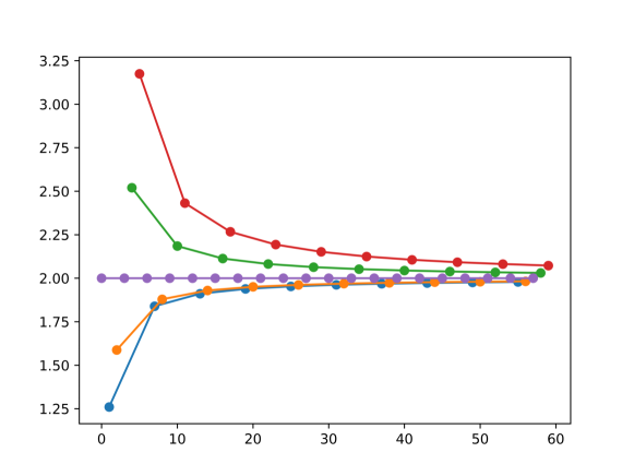
Figure 9. The norms of $\|T_{6n+l}^{{\mathsf{E}}_{3}}\|_{{\mathsf{E}}_{3}}$ for $0\leq n\leq 4$ and $0\leq l\leq 5$.

In the next section we shall prove that if $P_{n}^{\mu_{{\mathsf{E}}_{m}}}$ denotes the monic orthogonal polynomial with respect to equilibrium measure $\mu_{{\mathsf{E}}_{m}}$, then

$$n\mapsto\|P_{2nm+l}^{\mu_{{\mathsf{E}}_{m}}}\|^{2}_{L^{2}(\mu_{{\mathsf{E}}_{m}})}$$ (4.4)

is monotonic for any fixed $l$. In fact, this sequence increases when $l/m<1$ and decreases for $l/m>1$. This matches the numerically suggested behavior for the sup-norms of the Chebyshev polynomials.

5. Related orthogonal polynomials

We now turn our attention to the orthogonal polynomials with respect to the equilibrium measure of ${\mathsf{E}}_{m}$. Recall that if $\mu$ is a probability measure supported on the outer boundary of ${\mathsf{E}}_{m}$, then $\mu=\mu_{{\mathsf{E}}_{m}}$ precisely when (1.2) holds. With this result at hand, we can explicitly determine $\mu_{{\mathsf{E}}_{m}}$ (see also [32]).

Lemma 4.

Let ${\mathsf{E}}_{m}$ be defined as in (1.15). The equilibrium measure of ${\mathsf{E}}_{m}$ is absolutely continuous with respect to arc length measure and given by

$$d\mu_{{\mathsf{E}}_{m}}(z)=\frac{|z^{m-1}|}{\pi\sqrt{4-z^{2m}}}|dz|,\quad z\in{\mathsf{E}}_{m}.$$ (5.1)

Proof.

A straightforward computation shows that the measure defined in (5.1) is a probability measure on ${\mathsf{E}}_{m}$. We proceed to show that it satisfies (1.2). Note that if $\zeta,z\in\mathbb{C}$ then

$$\log|\zeta-z^{m}|=\sum\log|\zeta^{1/m}-z|,$$

where the sum is taken over all the $m$th roots of $\zeta$. Using this, we can compute the potential for the measure in question and arrive at

$$\frac{1}{\pi}\int_{{\mathsf{E}}_{m}}\log|x-z|\frac{|x^{m-1}|}{\sqrt{4-x^{2m}}}|dx| =\frac{1}{\pi}\sum_{k=1}^{2m}\int_{0}^{2^{1/m}}\log|e^{i\pi k/m}x-z|\frac{x^{m-1}}{\sqrt{4-x^{2m}}}dx$$

$$=\frac{1}{m\pi}\sum_{k=1}^{m}\int_{-2}^{2}\frac{\log|e^{i\pi k/m}t^{1/m}-z|}{\sqrt{4-t^{2}}}dt$$

$$=\frac{1}{m\pi}\int_{-2}^{2}\frac{\log|t-z^{m}|}{\sqrt{4-t^{2}}}dt=\frac{1}{m}G_{[-2,2]}(z^{m}).$$

The last equality follows from the fact that $dt/(\pi\sqrt{4-t^{2}})$ is the equilibrium measure of $[-2,2]$ which is a set of logarithmic capacity one. By Lemma LABEL:pre, we have

$$\frac{1}{m}G_{[-2,2]}(z^{m})=G_{{\mathsf{E}}_{m}}(z)$$

and consequently (5.1) holds true since also $\operatorname{Cap}({\mathsf{E}}_{m})=1$. ∎

As in Section 1.2, we shall use the notation $P_{n}^{\mu_{{\mathsf{E}}_{m}}}$ for the monic orthogonal polynomials with respect to $\mu_{{\mathsf{E}}_{m}}$. Recall that these polynomials minimise the integrals

$$\int_{{\mathsf{E}}_{m}}\left|P_{n}\right|^{2}d\mu_{{\mathsf{E}}_{m}}$$

among all monic polynomials of degree $n$. Just as in Lemma 3, one can use the symmetries of ${\mathsf{E}}_{m}$ to show that for $n,l\in{\mathbb{N}}$ and $0\leq l<2m$, we have

$$P_{2nm+l}^{\mu_{{\mathsf{E}}_{m}}}(z)=z^{2nm+l}+\sum_{k=0}^{n-1}a_{2km+l}z^{2km+l},\quad a_{2km+l}\in\mathbb{R}.$$ (5.2)

We are now ready to prove Theorem 4.

Proof of Theorem 4.

Fix $m\geq 2$, let $n\in{\mathbb{N}}$ and suppose $0\leq l<2m$. By Lemma 4 and with $P_{2nm+l}^{\mu_{{\mathsf{E}}_{m}}}$ as in (5.2), we have

$$\|P_{2nm+l}^{\mu_{{\mathsf{E}}_{m}}}\|_{L^{2}(\mu_{{\mathsf{E}}_{m}})}^{2} =\frac{1}{\pi}\int_{{\mathsf{E}}_{m}}\left|z^{2nm+l}+\sum_{k=0}^{n-1}a_{2km+l}z^{2km+l}\right|^{2}\frac{|z^{m-1}|}{\sqrt{4-z^{2m}}}|dz|$$

$$=\frac{2m}{\pi}\int_{[0,{2^{1/m}}]}\left|z^{2nm}+\sum_{k=0}^{n-1}a_{2km+l}z^{2km}\right|^{2}\frac{|z^{m+2l-1}|}{\sqrt{4-z^{2m}}}|dz|$$

$$=\frac{1}{\pi}\int_{0}^{4}\left(x^{n}+\sum_{k=0}^{n-1}a_{2km+l}x^{k}\right)^{2}\frac{x^{l/m-1/2}}{\sqrt{4-x}}dx.$$ (5.3)

Realising that the above integral is minimised precisely for the Jacobi polynomials (suitably rescaled to $[0,4]$), we can compute it explicitly. Following Szegő [48, Chapter IV], we adopt the notation

$$P_{n}^{(\alpha,\beta)}(x)={n+\alpha\choose n}{}_{2}F_{1}\left(-n,n+\alpha+\beta+1;\alpha+1;\frac{1-x}{2}\right)$$

and note that the leading coefficient of $P_{n}^{(\alpha,\beta)}$ is given by

$$2^{-n}{2n+\alpha+\beta\choose n}=\frac{\Gamma(2n+\alpha+\beta+1)}{2^{n}\Gamma(n+1)\Gamma(n+\alpha+\beta+1)}.$$

The integral in (5) can thus be written as

$$\quad\frac{2^{4n+l/m}\Gamma(n+1)^{2}\Gamma(n+l/m)^{2}}{\pi\Gamma(2n+l/m)^{2}}\int_{-1}^{1}\left(P_{n}^{(-1/2,l/m-1/2)}(x)\right)^{2}(1-x)^{-{1}/{2}}(1+x)^{l/m-1/2}dt\\ =\frac{2^{4n+2l/m}\Gamma(n+{1}/{2})\Gamma(n+1)\Gamma(n+{l}/{m})\Gamma(n+{l}/{m}+1/2)}{\pi(2n+{l}/{m})\Gamma(2n+l/m)^{2}}\quad$$ (5.4)

since

$$\int_{-1}^{1}\left(P_{n}^{(\alpha,\beta)}(x)\right)^{2}(1-x)^{\alpha}(1+x)^{\beta}dx=\frac{2^{\alpha+\beta+1}\Gamma(n+\alpha+1)\Gamma(n+\beta+1)}{(2n+\alpha+\beta+1)\Gamma(n+1)\Gamma(n+\alpha+\beta+1)}.$$

Applying Legendre’s duplication formula, the expression in (5.4) reduces to

$$\frac{2\Gamma(2n+1)\Gamma(2n+2l/m)}{(2n+l/m)\Gamma(2n+l/m)^{2}}$$

and recalling that $\Gamma(x+a)/\Gamma(x+b)\sim x^{a-b}$ as $n\to\infty$, we deduce that

$$\|P_{2nm+l}^{\mu_{{\mathsf{E}}_{m}}}\|_{L^{2}(\mu_{{\mathsf{E}}_{m}})}^{2}\to 2\;\mbox{ as }\;n\to\infty.$$

In order to prove the claimed monotonicity along subsequences, we introduce the quantity

$$\gamma_{n}(s):=\frac{2\Gamma(2n+1)\Gamma(2n+2s)}{(2n+s)\Gamma(2n+s)^{2}},\quad s\geq 0.$$

Note that $\|P_{2nm+l}^{\mu_{{\mathsf{E}}_{m}}}\|_{L^{2}(\mu_{{\mathsf{E}}_{m}})}^{2}=\gamma_{n}({l}/{m})$ and

$$\frac{\gamma_{n+1}(s)}{\gamma_{n}(s)} =\frac{\Gamma(2n+3)\Gamma(2n+2s+2)(2n+s)\Gamma(2n+s)^{2}}{\Gamma(2n+1)\Gamma(2n+2s)(2n+s+2)\Gamma(2n+s+2)^{2}}$$

$$=\frac{(2n+1)(2n+2)(2n+2s)(2n+2s+1)}{(2n+s)(2n+s+1)^{2}(2n+s+2)}.$$

Since

$$\frac{(x+1)(x+2s)}{(x+s)(x+s+1)}=\frac{x^{2}+2xs+x+2s}{x^{2}+2xs+x+s^{2}+s}$$

and

$$\frac{2s}{s^{2}+s}=\frac{2}{s+1}\gtrless 1\;\mbox{ for }\;s\lessgtr 1,$$

it follows that $\gamma_{n+1}(s)/\gamma_{n}(s)\gtrless 1$ for $s\lessgtr 1$. In this way, we have obtained the desired monotonicity statement. ∎

The sets ${\mathsf{E}}_{m}$ appear to be the first examples beyond the framework of single Jordan arcs for which (1.24) is fulfilled. We wonder how far one can push the conditions on ${\mathsf{E}}$ in the conjecture of [18].

6. A further investigation regarding ${\mathcal{W}}_{2n+1}({\mathsf{E}}_{2})$

The plot in Figure 4 indicates that $\|T_{2n+1}^{{\mathsf{E}}_{2}}\|_{{\mathsf{E}}_{2}}\lessgtr 2$ depending on whether $n$ is even or odd. As proven in Section 3, $T_{4n+l}^{{\mathsf{E}}_{2}}$ has a zero of order $l$ at $z=0$ (for $l=1,3$). However, there is no apparent explanation for why a zero with greater multiplicity would necessarily result in a higher sup-norm. In this section we shall study the preimages defined in (3.3) in more detail and try to shed more light on the pattern revealed by Figure 4.

As explained in Section 3, ${\mathsf{E}}_{2}^{n,l}$ consists of the base set ${\mathsf{E}}_{2}$ together with certain “decorations”. At all the points where $T_{4n+l}^{{\mathsf{E}}_{2}}$ has a zero, a new “crossing” will appear and each of the four preimages

$$(T_{4n+l}^{{\mathsf{E}}_{2}})^{-1}\Bigl{(}i^{k}\bigl{[}0,\|T_{4n+l}^{{\mathsf{E}}_{2}}\|_{{\mathsf{E}}_{2}}\bigr{]}\Bigr{)},\quad k=0,1,2,3$$ (6.1)

consists of $4n+l$ arcs. While $2n+1$ of these arcs lie on ${\mathsf{E}}_{2}$, the remaining $2n+l-1$ are orthogonal to ${\mathsf{E}}_{2}$ (except for the $l-1$ arcs emanating at the origin). It can be shown that every arc in ${\mathsf{E}}_{2}^{n,l}$ has harmonic measure equal to ${1}/{4(4n+l)}$, for instance, by examining a conformal map from ${\mathbb{C}}\setminus{\mathsf{E}}_{2}^{n,l}$ onto ${\mathbb{C}}\setminus\overline{{\mathbb{D}}}$. The typical shape of an ${\mathsf{E}}_{2}^{n,l}$ set is illustrated in Figures 11–11 below.

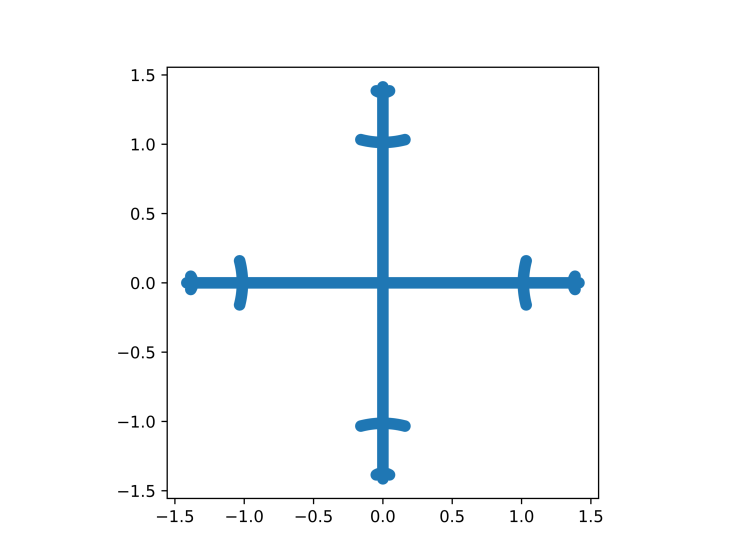
Figure 10. ${\mathsf{E}}_{2}^{2,1}$

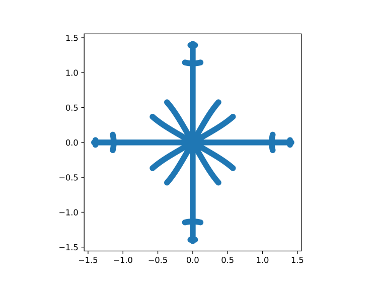
Figure 11. ${\mathsf{E}}_{2}^{2,3}$

With (3.5) in mind, we see that understanding the behaviour of $\|T_{4n+l}^{{\mathsf{E}}_{2}}\|_{{\mathsf{E}}_{2}}$ equates to effectively estimating the capacity of ${\mathsf{E}}_{2}^{n,l}$. Since the zeros of $T_{4n+l}^{{\mathsf{E}}_{2}}$ are hard to determine explicitly, it seems difficult to estimate this capacity directly. We get a better picture by considering the conformal map

$$\Phi(z)=\sqrt{{z^{2}}/{2}+\sqrt{\left({z^{2}}/{2}\right)^{2}-1}\,}$$

which maps ${\mathbb{C}}\setminus{\mathsf{E}}_{2}$ onto ${\mathbb{C}}\setminus\overline{{\mathbb{D}}}$. When applying $\Phi$, the complement of ${\mathsf{E}}_{2}^{n,l}$ is mapped onto the complement of the closed unit disk accompanied by certain “protrusions”, see Figures 13–13.

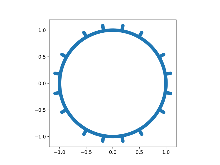
Figure 12. $\Phi({\mathsf{E}}_{2}^{2,1})$

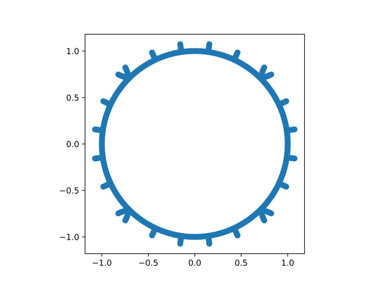
Figure 13. $\Phi({\mathsf{E}}_{2}^{2,3})$

By construction, all these $4(2n+l-1)$ protrusions have the same equilibrium measure relative to $\Phi({\mathsf{E}}_{2}^{n,l})$. Hence their combined mass relative to equilibrium measure amounts to

$$\frac{2n+l-1}{4n+l}.$$ (6.2)

As we shall argue below, the fact that this quantity is $<1/2$ for $l=1$ but $>1/2$ for $l=3$ seems to explain why $\|T_{2n+1}^{{\mathsf{E}}_{2}}\|_{{\mathsf{E}}_{2}}\lessgtr 2$ for $n$ even and odd, respectively.

Consider the sets

$$S(n,l):=\partial\mathbb{D}\,\cup\bigcup_{k=1}^{4(2n+l-1)}\exp\Bigl{\{}\frac{\pi ik/2}{2n+l-1}\Bigr{\}}\,[1,R_{n,l}],$$ (6.3)

where $R_{n,l}>1$ is a suitable constant depending on $n$ and $l$. These sets have a straightforward structure, allowing us to compute their capacity, and they also bear a resemblance to the configuration of $\Phi({\mathsf{E}}_{2}^{n,l})$. Although it may seem that way at first glance, the protrusions in $\Phi({\mathsf{E}}_{2}^{n,l})$ are not perfectly straight line segments, and their distribution on $\partial{\mathbb{D}}$ is not entirely uniform. One can show that by selecting $R_{n,l}$ in such a way that

$$\mu_{S(n,l)}(\partial{\mathbb{D}})=\frac{2n+1}{4n+l},$$ (6.4)

the inequality $\operatorname{Cap}(S(n,l))^{4n+l}\lessgtr\sqrt{2}$ holds, depending on whether $l=1$ or $3$. For example, by performing a straightforward calculation, we find that

$$\operatorname{Cap}\bigl{(}S(n,1)\bigr{)}={\Bigl{(}\cos\Bigl{(}\frac{\pi n}{4n+1}\Bigr{)}\Bigr{)}}^{-1/4n}$$

and from this expression, one can infer that $\operatorname{Cap}(S(n,1))^{4n+1}\to\sqrt{2}$ in a monotonically increasing manner. Taking (3.5) into account, we now possess additional evidence indicating that $\|T_{4n+1}^{{\mathsf{E}}_{2}}\|_{{\mathsf{E}}_{2}}\to 2$ from below. Similar reasoning provides support for the conjecture that $\|T_{4n+3}^{{\mathsf{E}}_{2}}\|_{{\mathsf{E}}_{2}}\to 2$ from above.

7. Outlook and perspective

A key finding of this paper has been to show that, beyond intervals, there exist compact subsets of ${\mathbb{C}}$ for which the Widom factors converge to $2$. Specifically, the sets ${\mathsf{E}}_{m}$ as defined in Theorem 2 and illustrated in Figures 3–3 exhibit this property when $m\geq 2$, and the same holds for any other symmetric star graph with an odd number of edges. It is reasonable to inquire whether or not there are more sets ${\mathsf{E}}\subset{\mathbb{C}}$ for which ${\mathcal{W}}_{n,\infty}({\mathsf{E}})\to 2$. As explained below, we believe the answer is indeed affirmative.

Recall that if $P$ is a complex polynomial and $P^{\prime}(z)=0$, then $z$ is called a critical point and $w=P(z)$ a critical value for $P$. Polynomials with at most two critical values, say $c_{1}$ and $c_{2}$, are known as Shabat polynomials (or generalised Chebyshev polynomials), see [10, 41]. Since this class of polynomials is invariant under non-degenerate linear transformations, we may assume that $c_{1}=-2$ and $c_{2}=2$. It is a known fact (see, e.g., [10] or [26]) that for Shabat polynomials, the preimage $P^{-1}([-2,2])$ is a planar tree with as many edges as the degree of $P$. In fact, one can establish a bijection between the set of bicolored planer trees and the set of equivalence classes of Shabat polynomials. Moreover, with respect to the point at $\infty$, every edge of $P^{-1}([-2,2])$ has equal harmonic measure and any subset of an edge has equal harmonic measure from both sides. Trees with these properties are also called “balanced trees” and they satisfy the $S$-property of Definition 1. A remarkable result of Bishop [11] shows that balanced trees are dense in all planar continua (i.e., compact connected subsets of ${\mathbb{C}}$) with respect to the Hausdorff metric.

For $n\geq 2$, the polynomial $P_{n}(z)=z^{n}$ has one critical point (namely, $z=0$) and one critical value $w=0$. So the preimage $P_{n}^{-1}([0,4])$ is a balanced tree and when $n=2m$, this tree coincides with ${\mathsf{E}}_{m}$ as defined in (1.15). Another example of a Shabat polynomial (with critical values $w=0,1$) is

$$P(z)=\frac{8}{729}(z+1)\Bigl{(}z^{2}-\frac{3}{2}z+\frac{9}{2}\Bigr{)}^{3}$$

and the corresponding tree is pictured in Figure 15. By use of the algorithm mentioned in Section 3, one can compute the norms of $T_{n}^{{\mathsf{E}}_{P}}$ for degree up to $40$ with a precision of $10^{-2}$. The outcome is illustrated in Figure 15.

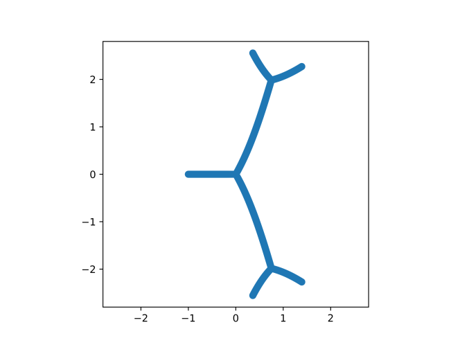
Figure 14. ${\mathsf{E}}_{P}=P^{-1}([0,1])$

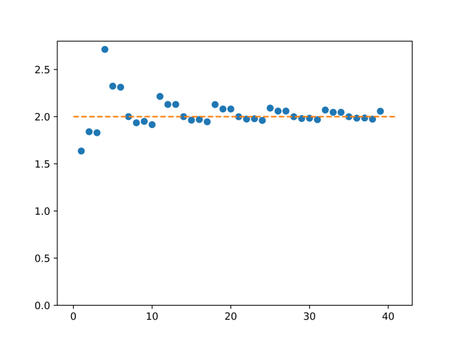
Figure 15. Widom factors for ${{\mathsf{E}}_{P}}$

Similar plots for other Shabat polynomials lead to the same pattern and we thus have the courage to hypothesize that the first part of Theorem 2 applies to all balanced trees.

Conjecture 1.

Let $P$ be a monic Shabat polynomial with critical values in $\{-2,2\}$ and consider the preimage ${\mathsf{E}}_{P}:=P^{-1}([-2,2])$. Then

$$\lim_{n\to\infty}{\mathcal{W}}_{n,\infty}({\mathsf{E}}_{P})=2.$$

Since any balanced tree satisfies the $S$-property, one may speculate if this conjecture can be extended to a larger class of sets. In fact, if the property of every edge having equal harmonic measure turns out to not play a role, it would be natural to formulate the conjecture for so-called generalised Shabat polynomials. This class was introduced in [26] and allows for more than two critical values as long as they all belong to $[-2,2]$. The preimage $P^{-1}([-2,2])$ is connected (in fact, a tree) if and only if $[-2,2]$ contains all the critical values of $P$. The ideal scenario would be that the conjecture holds true for all connected sets characterised by the $S$-property.

Regrettably, our current method of proof does not exhibit a clear path for generalisation within the context of Shabat polynomials and the $S$-property. Novel strategies and ideas are required to advance our understanding in this domain.

Appendix A Bernstein’s method

In this appendix we shall discuss a proof of Theorem 5. Our approach will be a simplification of the method employed by Bernstein in [8]. The initial stage of [8] involved showing that if $w$ is a polynomial which is strictly positive on $[-1,1]$, then the monic orthogonal polynomials $P_{n}^{w}$ with respect to the weight function

$${w(x)}/{\sqrt{1-x^{2}}}$$

are well-suited trial polynomials for minimisation of the quantity

$$\max_{x\in[-1,1]}\left|\sqrt{w(x)}\left(x^{n}+\sum_{k=0}^{n-1}c_{k}x^{k}\right)\right|.$$

As in Section 3, we shall denote these minimisers by $T_{n}^{\sqrt{w}}$. More specifically, Bernstein proved that $\sqrt{w}P_{n}^{w}$ is asymptotically alternating for this class of polynomial weights and an explicit analysis of $P_{n}^{w}$ can then be used to unveil the asymptotic behaviour of $\|\sqrt{w}T_{n}^{\sqrt{w}}\|_{[-1,1]}$ as stated in Theorem 5.

Rather than using orthogonal polynomials as trial polynomials, we shall base our analysis on an explicit expression for certain weighted Chebyshev polynomials due to Achieser [2, Appendix A]. This formula is presented in Section A.1. Since the class of weights includes the reciprocal of any strictly positive polynomial on $[-1,1]$, we can — in line with Bernstein — apply a standard approximation argument to conclude that Theorem 5 holds true for all Riemann integrable weights on $[-1,1]$ which are bounded above and below by positive constants. This is the second step in the proof and we outline the details in Section A.2. The final and most complicated step is to allow for zeros of the weight function on $[-1,1]$. We shall present exactly the same refined argument as provided by Bernstein [8] in Section A.3.

A.1. An explicit formula for certain weighted Chebyshev polynomials

Denote by $\overline{{\mathbb{R}}}:={\mathbb{R}}\cup\{\infty\}$ the extended real line. Let $a_{k}\in\overline{{\mathbb{R}}}\setminus[-1,1]$ and form the product

$$w(x)=\prod_{k=1}^{2m}\left(1-\frac{x}{a_{k}}\right)^{-1/2},$$

which represents a positive weight function on $[-1,1]$. The case of an odd number of factors can be handled by taking $a_{2m}=\infty$ and $|a_{k}|<\infty$ for $k=1,2,\ldots,2m-1$. Let $z\in\partial{\mathbb{D}}$ and $\rho_{k}\in{\mathbb{D}}$ be defined implicitly by

$$x=\frac{1}{2}\left(z+\frac{1}{z}\right)\;\mbox{ and }\;a_{k}=\frac{1}{2}\left(\rho_{k}+\frac{1}{\rho_{k}}\right)\;\mbox{ for }\;k=1,2,\ldots,2m.$$

The following explicit representation for $wT_{n}^{w}$ is given by Achieser [2, Appendix A].

Theorem A.1.

For $n>m$, we have

$$w(x)T_{n}^{w}(x)=2^{-n}\prod_{k=1}^{2m}\sqrt{1+\rho_{k}^{2}}\left(z^{m-n}\prod_{k=1}^{2m}\sqrt{\frac{1-z\rho_{k}}{z-\rho_{k}}}+z^{n-m}\prod_{k=1}^{2m}\sqrt{\frac{z-\rho_{k}}{1-z\rho_{k}}}\,\right)$$ (A.1)

and

$$\|wT_{n}^{w}\|_{[-1,1]}=2^{1-n}\exp\left\{\frac{1}{\pi}\int_{-1}^{1}\frac{\log w(x)}{\sqrt{1-x^{2}}}dx\right\}.$$ (A.2)

Remark.

One can show that the expression on the right-hand side of (A.1) indeed becomes a polynomial (in $x$) after division by $w(x)$. Moreover, this polynomial satisfies the orthogonality conditions

$$\int_{-1}^{1}T_{n}^{w}(x)x^{k}\frac{w(x)^{2}}{\sqrt{1-x^{2}}}dx=0,\quad k=0,1,\ldots,n-1$$

when $n\geq m$.

By letting $a_{2k}=a_{2k-1}$ for $k=1,2,\ldots,m$, we see that Theorem A.1 in particular applies to weights of the form

$$w(x)=\prod_{k=1}^{m}\left(1-\frac{x}{a_{k}}\right)^{-1}.$$

This was in fact already proven by Chebyshev [13].

A.2. Norm asymptotics for more general weighted Chebyshev polynomials

We now consider generalising (A.2) to the case where $w$ is merely a Riemann integrable function on $[-1,1]$ satisfying

$$\frac{1}{M}\leq w(x)\leq M$$ (A.3)

for some $M\geq 1$. In this more general setting, we no longer have equality. But the two expressions in (A.2) are still asymptotically equivalent as $n\to\infty$.

The idea is to approximate $w$ by reciprocals of polynomials. Set $\omega=1/w$ and choose sequences $\{\omega_{u}^{k}\}_{k}$ and $\{\omega_{l}^{k}\}_{k}$ of polynomials with real zeros away from $[-1,1]$ such that

$$\frac{1}{2M}\leq\omega_{u}^{k}(x)\leq\omega(x)\leq\omega_{l}^{k}(x)\leq 2M$$

and

$$\lim_{k\rightarrow\infty}\omega_{u}^{k}(x)=\omega(x)=\lim_{k\rightarrow\infty}\omega_{l}^{k}(x)$$

for every $x\in[-1,1]$. Defining $w_{l}^{k}=1/\omega_{l}^{k}$ and $w_{u}^{k}=1/\omega_{u}^{k}$, we obtain that

$$w_{l}^{k}(x)\leq w(x)\leq w_{u}^{k}(x)$$

while maintaining the pointwise convergence

$$\lim_{k\rightarrow\infty}w_{l}^{k}(x)=w(x)=\lim_{k\rightarrow\infty}w_{u}^{k}(x).$$

This in turn implies that

$$\|T_{n}^{w_{l}}w_{l}\|_{[-1,1]}\leq\|T_{n}^{w}w_{l}\|_{[-1,1]}\leq\|T_{n}^{w}w\|_{[-1,1]}\leq\|T_{n}^{w_{u}}w\|_{[-1,1]}\leq\|T_{n}^{w_{u}}w_{u}\|_{[-1,1]}.$$ (A.4)

Furthermore, using dominated convergence we get that

$$\lim_{k\rightarrow\infty}\int_{-1}^{1}\frac{\log w_{l}^{k}(x)}{\sqrt{1-x^{2}}}dx=\int_{-1}^{1}\frac{\log w(x)}{\sqrt{1-x^{2}}}dx=\lim_{k\rightarrow\infty}\int_{-1}^{1}\frac{\log w_{u}^{k}(x)}{\sqrt{1-x^{2}}}dx$$

and for any given $\epsilon>0$, we can therefore choose $k$ large enough that

$$\left|\exp\left\{\frac{1}{\pi}\int_{-1}^{1}\frac{\log w_{i}^{k}(x)}{\sqrt{1-x^{2}}}dx\right\}-\exp\left\{\frac{1}{\pi}\int_{-1}^{1}\frac{\log w(x)}{\sqrt{1-x^{2}}}dx\right\}\right| <\epsilon,\quad i=l,u.$$

For $n$ sufficiently large, Theorem A.1 implies that

$$\|T_{n}^{w_{i}^{k}}w_{i}^{k}\|_{[-1,1]}=2^{1-n}\exp\left\{\frac{1}{\pi}\int_{-1}^{1}\frac{\log w_{i}^{k}(x)}{\sqrt{1-x^{2}}}dx\right\},\quad i=l,u.$$

By combining this with (A.4), we thus get the inequalities

$$\exp\left\{\frac{1}{\pi}\int_{-1}^{1}\frac{\log w(x)}{\sqrt{1-x^{2}}}dx\right\}-\epsilon\leq 2^{n-1}\|T_{n}^{w}w\|_{[-1,1]}\leq\exp\left\{\frac{1}{\pi}\int_{-1}^{1}\frac{\log w(x)}{\sqrt{1-x^{2}}}dx\right\}+\epsilon.$$

As $\epsilon>0$ is arbitrary, we conclude that

$$\|T_{n}^{w}w\|_{[-1,1]}=2^{1-n}\exp\left\{\frac{1}{\pi}\int_{-1}^{1}\frac{\log w(x)}{\sqrt{1-x^{2}}}dx\right\}\bigl{(}1+o(1)\bigr{)}$$ (A.5)

as $n\rightarrow\infty$. This proves Theorem 5 when $w$ is Riemann integrable and satisfies (A.3).

A.3. Allowing for zeros of the weight function

The final step in proving Theorem 5 is to allow for zeros at certain points of $[-1,1]$. We will adopt the approach outlined in [8] and restrict our examination to the introduction of a single zero $b_{1}=b$ within the interval $[-1,1]$ using the weight $|x-b|^{\alpha}$. That is, we consider weights of the form

$$w(x)=w_{0}(x)|x-b|^{\alpha},$$ (A.6)

where $w_{0}$ is Riemann integrable and satisfies $1/M\leq w_{0}(x)\leq M$ for some constant $M\geq 1$. More zeros can be added by repeated use of the argument we are about to explain.

Assume first that $\alpha=m$ is a positive integer. For ${\epsilon}>0$, consider the weight function

$$w^{\epsilon}(x)=w_{0}(x)|x-b-i{\epsilon}|^{m}.$$

This weight is non-vanishing on $[-1,1]$ and fulfils all the previous requirements for (A.5) to be valid. By use of Lemma 2, we hence find that

$$\|T_{n}^{w^{\epsilon}}w^{\epsilon}\|_{[-1,1]} =2^{1-n}\exp\left\{\frac{1}{\pi}\int_{-1}^{1}\frac{\log w_{0}(x)}{\sqrt{1-x^{2}}}dx\right\}\exp\left\{\frac{1}{\pi}\int_{-1}^{1}\frac{\log|x-b-i{\epsilon}|^{m}}{\sqrt{1-x^{2}}}dx\right\}\bigl{(}1+o(1)\bigr{)}$$

$$=\|T_{n}^{w_{0}}w_{0}\|_{[-1,1]}\Biggl{(}\frac{\left|(b+i{\epsilon})+\sqrt{(b+i{\epsilon})^{2}-1}\right|}{2}\Biggr{)}^{m}\bigl{(}1+o(1)\bigr{)}$$ (A.7)

as $n\to\infty$. Note that the second factor in (A.7) converges to $2^{-m}$ as ${\epsilon}\rightarrow 0$. Since $w^{\epsilon}>w$ on $[-1,1]$, we deduce as in (A.4) that

$$\begin{split}\|T_{n}^{w^{\epsilon}}w^{\epsilon}\|_{[-1,1]}&\geq\|T_{n}^{w^{\epsilon}}w\|_{[-1,1]}\geq\|T_{n}^{w}w\|_{[-1,1]}\\ &\geq\|T_{n+m}^{w_{0}}w_{0}\|_{[-1,1]}=2^{-m}\|T_{n}^{w_{0}}w_{0}\|_{[-1,1]}\bigl{(}1+o(1)\bigr{)}.\end{split}$$ (A.8)

The combination of (A.7) and (A.8) now implies that

$$\|T_{n}^{w}w\|_{[-1,1]}=2^{-m}\|T_{n}^{w_{0}}w_{0}\|_{[-1,1]}\bigl{(}1+o(1)\bigr{)}=2^{1-n}\exp\left\{\frac{1}{\pi}\int_{-1}^{1}\frac{\log w(x)}{\sqrt{1-x^{2}}}dx\right\}\bigl{(}1+o(1)\bigr{)}$$

as $n\to\infty$, and this proves that (A.5) is valid for weights of the form (A.6) with $\alpha=m\in{\mathbb{N}}$.

We next consider the case of negative integer powers. If $\alpha=-m$ is a negative integer, then $T_{n+m}^{w}$ has a zero of order $m$ at $x=b$ and hence

$$T_{n+m}^{w}(x)w(x)=T_{n}^{w_{0}}(x)w_{0}(x)\frac{(x-b)^{m}}{|x-b|^{m}}.$$

Therefore,

$$\|T_{n+m}^{w}w\|_{[-1,1]} =2^{1-n}\exp\left\{\frac{1}{\pi}\int_{-1}^{1}\frac{\log w_{0}(x)}{\sqrt{1-x^{2}}}dx\right\}\bigl{(}1+o(1)\bigr{)}$$

$$=2^{1-n-m}\exp\left\{\frac{1}{\pi}\int_{-1}^{1}\frac{\log w(x)}{\sqrt{1-x^{2}}}dx\right\}\bigl{(}1+o(1)\bigr{)}$$

as $n\to\infty$, and this proves the validity of (A.5) for such weights as well.

To handle arbitrary exponents $\alpha\in\mathbb{R}$, it suffices to examine the case of $\alpha\in(0,1)$. The weight function $w_{0}$ can namely incorporate zeros with integer exponents on $[-1,1]$ as we have already addressed the asymptotics in this particular case. Let ${\epsilon}>0$ and form the weight functions

$$w_{l}^{{\epsilon}}(x) =\begin{cases}w(x),&|x-b|\geq{\epsilon}\\ w_{0}(x)|x-b|,&|x-b|<{\epsilon},\end{cases}$$

$$w_{u}^{{\epsilon}}(x) =\begin{cases}w(x),&|x-b|\geq{\epsilon}\\ w_{0}(x),&|x-b|<{\epsilon}.\end{cases}$$

Note that (A.5) applies to both $w_{l}^{{\epsilon}}$ and $w_{u}^{{\epsilon}}$. Regardless of the value of $0<{\epsilon}<1$, we have the inequalities

$$w_{l}^{{\epsilon}}(x)\leq w(x)\leq w_{u}^{{\epsilon}}(x)$$

and hence

$$\|T_{n}^{w_{l}^{{\epsilon}}}w_{l}^{{\epsilon}}\|_{[-1,1]}\leq\|T_{n}^{w}w\|_{[-1,1]}\leq\|T_{n}^{w_{u}^{{\epsilon}}}w_{u}^{{\epsilon}}\|_{[-1,1]}.$$

Consequently,

$$\qquad 2^{1-n}\exp\left\{\frac{1}{\pi}\int_{-1}^{1}\frac{\log w_{l}^{{\epsilon}}(x)}{\sqrt{1-x^{2}}}dx\right\}\bigl{(}1+o(1)\bigr{)}\\ \leq\|T_{n}^{w}w\|_{[-1,1]}\leq 2^{1-n}\exp\left\{\frac{1}{\pi}\int_{-1}^{1}\frac{\log w_{u}^{{\epsilon}}(x)}{\sqrt{1-x^{2}}}dx\right\}\bigl{(}1+o(1)\bigr{)}\qquad$$

as $n\rightarrow\infty$. By dominated convergence,

$$\lim_{{\epsilon}\rightarrow 0}\int_{-1}^{1}\frac{\log w_{l}^{{\epsilon}}(x)}{\sqrt{1-x^{2}}}dx=\int_{-1}^{1}\frac{\log w(x)}{\sqrt{1-x^{2}}}dx=\lim_{{\epsilon}\rightarrow 0}\int_{-1}^{1}\frac{\log w_{u}^{{\epsilon}}(x)}{\sqrt{1-x^{2}}}dx,$$

so for any given $r>0$, we can choose ${\epsilon}>0$ small enough that

$$1-r\leq\frac{\exp\left\{\frac{1}{\pi}\int_{-1}^{1}\frac{\log w_{l}^{{\epsilon}}(x)}{\sqrt{1-x^{2}}}dx\right\}}{\exp\left\{\frac{1}{\pi}\int_{-1}^{1}\frac{\log w(x)}{\sqrt{1-x^{2}}}dx\right\}}\leq 1,\qquad 1\leq\frac{\exp\left\{\frac{1}{\pi}\int_{-1}^{1}\frac{\log w_{u}^{{\epsilon}}(x)}{\sqrt{1-x^{2}}}dx\right\}}{\exp\left\{\frac{1}{\pi}\int_{-1}^{1}\frac{\log w(x)}{\sqrt{1-x^{2}}}dx\right\}}\leq 1+r.$$

This in turn implies that

$$\qquad 2^{1-n}\exp\left\{\frac{1}{\pi}\int_{-1}^{1}\frac{\log w(x)}{\sqrt{1-x^{2}}}dx\right\}(1-r)\bigl{(}1+o(1)\bigr{)}\\ \leq\|T_{n}^{w}w\|_{[-1,1]}\leq 2^{1-n}\exp\left\{\frac{1}{\pi}\int_{-1}^{1}\frac{\log w(x)}{\sqrt{1-x^{2}}}dx\right\}(1+r)\bigl{(}1+o(1)\bigr{)}\qquad$$

as $n\rightarrow\infty$. Since $r>0$ is arbitrary, we conclude that

$$\|T_{n}^{w}w\|_{[-1,1]}=2^{1-n}\exp\left\{\frac{1}{\pi}\int_{-1}^{1}\frac{\log w(x)}{\sqrt{1-x^{2}}}dx\right\}\bigl{(}1+o(1)\bigr{)}$$

as $n\rightarrow\infty$. In other words, (A.5) — which coincides with (3.9) — applies. The addition of more weights of the form $|x-b_{k}|^{\alpha_{k}}$ can be carried out by repeated use of the argument explained above.

References

- [1] N. I. Achieser, Über einige Funktionen, welche in zwei gegebenen Intervallen am wenigsten von Null abweichen, I–II. Bull. Acad. Sci. URSS 9 (1932) 1163–1202; 3 (1933) 309–344.
- [2] N. I. Achieser, Theory of Approximation, Frederick Ungar Publishing Co., New York, 1956.
- [3] G. Alpan, Extremal polynomials on a Jordan arc, J. Approx. Theory 276 (2022) 105708.
- [4] G. Alpan and M. Zinchenko, On the Widom factors for extremal polynomials, J. Approx. Theory 259 (2020) 105480.
- [5] V. V. Andrievskii, Chebyshev polynomials on a system of continua, Constr. Approx. 43 (2016) 217–229.
- [6] V. V. Andrievskii, On Chebyshev polynomials in the complex plane, Acta Math. Hungar. 152 (2017) 505–524.
- [7] D. Armitage and S. J. Gardiner, Classical Potential Theory, Springer-Verlag, London, 2001.
- [8] S. N. Bernstein, Sur les polynômes orthogonaux relatifs à un segment fini, J. Math. 9 (1930) 127–177; 10 (1931) 219–286.
- [9] H. P. Blatt, E. B. Saff, and M. Simkani, Jentzsch–Szegő type theorems for the zeros of best approximants, J. London Math. Soc. 38 (1988), 307–316.
- [10] J. Bétréma and A. K. Zvonkin, Plane trees and Shabat polynomials, Discrete Math. 153 (1996) 47–58.
- [11] C. J. Bishop, True trees are dense, Invent. Math. 197 (2014) 433–452.
- [12] P. L. Chebyshev, Théorie des mécanismes connus sous le nom de parallélogrammes, Mém. des sav. étr. prés. à l’Acad. de. St. Pétersb. 7 (1854) 539–568.
- [13] P. L. Chebyshev, Sur les questions de minima qui se rattachent à la représentation approximative des fonctions, Mém. Acad. St. Pétersb. 7 (1859) 199–291.
- [14] J. S. Christiansen, B. Simon, and M. Zinchenko, Asymptotics of Chebyshev polynomials, I. Subsets of , Invent. Math. 208 (2017) 217–245.
- [15] J. S. Christiansen, B. Simon, P. Yuditskii, and M. Zinchenko, Asymptotics of Chebyshev polynomials, II. DCT subsets of , Duke Math. J. 168 (2019) 325–349.
- [16] J. S. Christiansen, B. Simon, and M. Zinchenko, Asymptotics of Chebyshev polynomials, III. Sets saturating Szegő, Schiefermayr, and Totik–Widom bounds, Oper. Theory Adv. Appl. 276 (2020) 231–246.
- [17] J. S. Christiansen, B. Simon, and M. Zinchenko, Asymptotics of Chebyshev polynomials, IV. Comments on the complex case, JAMA 141 (2020) 207–223.
- [18] J. S. Christiansen, B. Simon, and M. Zinchenko, Widom factors and Szegő–Widom asymptotics, a review, Oper. Theory Adv. Appl. 289 (2022) 301–319.
- [19] B. Eichinger, Szegő–Widom asymptotics of Chebyshev polynomials on circular arcs, J. Approx. Theory 217 (2017) 15–25.
- [20] G. Faber, Über Tschebyscheffsche Polynome, J. Reine Angew. Math. 150 (1919) 79–106.
- [21] M. Fekete, Über die Verteilung der Wurzeln bei gewissen algebraischen Gleichungen mit ganzzahligen Koeffizienten, Math. Z. 17 (1923) 228–249.
- [22] B. Fischer and J. Modersitzki, An algorithm for complex linear approximation based on semi-infinite programming, Numer. Algorithms 5 (1993) 287–297.
- [23] J. B. Garnett and D. E. Marshall, Harmonic Measure, New Mathematical Monographs, Cambridge University Press, 2005.
- [24] H. Grötzsch, Über ein Variationsproblem der konformen Abbildung, Ber. Ferh. Sächs. Akad. Wiss. Leipzig 82 (1930) 251–263.
- [25] L. Helms, Potential Theory, Springer-Verlag, London, 2009.
- [26] G. Jensen and C. Pommerenke, Shabat polynomials and conformal mappings, Acta Sci. Math. (Szeged) 85 (2019) 147–170.
- [27] S. O. Kamo and P. A. Borodin, Chebyshev polynomials for Julia sets, Moscow Univ. Math. Bull. 49 (1994) 44–45.
- [28] G. V. Kuz’mina, Moduli of families of curves and quadratic differentials, Proc. Steklov Inst. Math. 139 (1982) 1–231.
- [29] N. S. Landkof, Foundations of Modern Potential Theory, Springer-Verlag, New York–Heidelberg, 1972.
- [30] G. G. Lorentz, Approximation of Functions, Chelsea, New York, 1986.
- [31] A. Mart∞́nez-Finkelshtein, E. A. Rakhmanov, and S. P. Suetin, Variation of the equilibrium energy and the -property of stationary compact sets, Sb. Math. 202 (2011) 1831–1852.
- [32] F. Peherstorfer and R. Steinbauer, Orthogonal and -extremal polynomials on inverse images of polynomial mappings, J. Comput. Appl. Math. 127 (2001) 297–315.
- [33] G. Pólya, Beitrag zur Verallgemeinerung des Verzerrungssatzes auf mehrfach zusammenhängenden Gebieten, III. Sitzungsberichte Preuss. Akad. Wiss. Berlin, Phys.-Math. Kl. (1929) 55–62.
- [34] Ch. Pommerenke, Boundary Behavior of Conformal Maps, Springer-Verlag, Berlin, Heidelberg, New York, 1992.
- [35] T. Ransford, Potential Theory in the Complex Plane, Cambridge University Press, Cambridge, 1995.
- [36] E. Remez, Sur la détermination des polynômes d’approximation de degré donnée, Comm. Soc. Math. Kharkov 10 (1934) 41–63.
- [37] E. Remez, Sur un procédé convergent d’approximations successives pour déterminer les polynômes d’approximation, Compt. Rend. Acad. Sc. 198 (1934) 2063–2065.
- [38] K. Schiefermayr, A lower bound for the minimum deviation of the Chebyshev polynomial on a compact real set, East J. Approx. 14 (2008) 223–233.
- [39] K. Schiefermayr, The Pólya–Chebotarev problem and inverse polynomial images, Acta Math. Hungar. 142 (2014) 80–94.
- [40] K. Schiefermayr, Chebyshev polynomials on circular arcs, Acta Sci. Math. 85 (2019) 629–649.
- [41] G. Shabat and A. Zvonkin, Plane trees and algebraic numbers, In: Jerusalem combinatorics ’93, Contemp. Math. 178 (1994) 233–275.
- [42] V. I. Smirnov and N. A. Lebedev, Functions of a Complex Variable: Constructive Theory, M.I.T. Press, Massachusetts Institute of Technology, Cambridge, 1968.
- [43] H. Stahl, Extremal domains associated with an analytic function, I–II. Complex Variables, Theory Appl. 4 (1985) 311–324; 325–338.
- [44] H. Stahl, The structure of extremal domains associated with an analytic function, Complex Variables, Theory Appl. 4 (1985) 339–354.
- [45] H. Stahl, A potential-theoretic problem connected with complex orthogonality, Contemp. Math. 507 (2010) 255–285.
- [46] H. Stahl, Sets of minimal capacity and extremal domains, arXiv:1205.3811
- [47] G. Szegő, Bemerkungen zu einer Arbeit von Herrn M. Fekete: Über die Verteilung der Wurzeln bei gewissen algebraischen Gleichungen mit ganzzahligen Koeffizienten, Math. Z. 21 (1924) 203–208.
- [48] G. Szegő, Orthogonal Polynomials, Vol. 23 of Amer. Math. Soc. Colloq. Publ., American Mathematical Society, Providence, RI, fourth edition, 1975.
- [49] P. Tang, A fast algorithm for linear complex Chebyshev approximations, Math. Comp. 51 (1988) 721–739.
- [50] J.-P. Thiran and C. Detaille, Chebyshev polynomials on circular arcs and in the complex plane, In: Progress in Approximation Theory, Academic Press, Boston, MA, 1991, pp. 771–786.
- [51] V. Totik, The norm of minimal polynomials on several intervals, J. Approx. Theory 163 (2011) 738–746.
- [52] V. Totik, Chebyshev polynomials on compact sets, Potential Anal. 40 (2014) 511–524.
- [53] V. Totik, Asymptotics of Christoffel functions on arcs and curves, Adv. Math. 252 (2014) 114–149.
- [54] H. Widom, Extremal polynomials associated with a system of curves in the complex plane, Adv. in Math. 3 (1969) 127–232.