Nuclear mass radius and pressure in the Skyrme model

Abstract

We compute the mass radius, scalar radius, tensor radius, baryon number radius and mechanical radius of nuclei with baryon number $B=1,2,3,4,5,6,7,8,32,108$ in the Skyrme model. The relations between these radii and the nuclear gravitational form factors are investigated. We also compute the ‘pressure’ distribution and find that it is negative in the core region for all the nuclei with $B>1$. This suggests that the way mechanical stability is achieved in nuclei is qualitatively different than in the nucleon.

I Introduction

Traditionally, since 1950s, the size of the proton has been determined through the measurement of the electromagnetic form factors in lepton-proton elastic scattering Hofstadter (1956). The charge radius thus extracted, about 0.8 fm, helps us to draw an intuitive picture of how quarks are distributed inside the proton. Its precise value is fundamentally important in QCD, QED and atomic spectroscopy. The same method can be used to define and determine the radius of atomic nuclei Hofstadter (1956); Frosch et al. (1968); De Vries et al. (1987); Sick (2008). After years of controversy known as the proton radius puzzle Carlson (2015); Gao and Vanderhaeghen (2022), the most recent measurements have finally found consistency between the results from electron scattering and muonic hydrogen (muonic atom) spectroscopy Pohl et al. (2010); Xiong et al. (2019); Krauth et al. (2021).

However, the charge radius is by no means the unique characterization of the size of hadrons and nuclei. For neutral hadrons, it may not be literally interpreted as a measure of physical size, as exemplified by the negative mean square radius of the neutron Kopecky et al. (1995). Even for charged hadrons, the charge radius does not fully reflect their internal structure. The virtual photon exchanged in electron scattering only sees quarks and does not probe gluons which are essential constituents of the target. It then appears reasonable and complementary to characterize the size of hadrons and nuclei in terms of the distribution of energy, angular momentum, etc., carried by quarks and gluons. This can be done by defining a radius through the gravitational form factors (GFFs), the off-forward matrix element of the QCD energy-momentum tensor $T^{\mu\nu}$ Kobzarev and (1962); Pagels (1966).

Since $T^{\mu\nu}$ has many components, one can define various radii with different physical interpretations Goeke et al. (2007); Cebulla et al. (2007). For example, the mass radius measures the distribution of the energy density $T^{00}({\bm{x}})$. Similarly, the scalar radius is associated with the QCD trace anomaly density $T^{\mu}_{\mu}({\bm{x}})$. An obvious question, however, is whether they are measurable in experiments. In fact, it is only recently that there have been new ideas and attempts at extracting the gravitational form factors and the associated radii Kumano et al. (2018); Burkert et al. (2018); Hatta and Yang (2018); Mamo and Zahed (2020); Kharzeev (2021); Sun et al. (2021); Duran et al. (2023); Wang et al. (2022); Guo et al. (2023); Wang et al. (2023); Adhikari et al. (2023); Hatta (2023). While at the moment the precision of such extractions falls behind that of the electromagnetic form factors, this is an encouraging development worth pursuing in the future, especially towards the era of the Electron-Ion Collider (EIC) Abdul Khalek et al. (2022).

Just like the charge radius, the discussion of the GFFs and associated radii can be extended to atomic nuclei. In a previous paper Garcia Martin-Caro et al. (2023), we have computed, for the first time, the GFFs of various nuclei within the Skyrme model Skyrme (1961). In this model, a nucleus is realized as a classical field configuration (‘Skyrmion’) with a definite baryon number $B$. The calculation of the GFFs is complicated by the fact that the classical solutions are not spherically symmetric for $B>1$, but we have successfully extracted one of the GFFs, the $D(t)$ form factor, for a variety of nuclei. We find that the so-called D-term $D(t=0)\sim B^{1.8}$ grows rapidly with increasing $B$. (Compare with the earlier works Polyakov (2003); Liuti and Taneja (2005); Guzey and Siddikov (2006) and a recent work He and Zahed (2023)).) As the D-term is commonly associated with the internal radial force, or ‘pressure’, it affects the size of the system. The goal of this paper is to systematically compute various definitions of radii for various nuclei, and study their connection to the D-term.

II Radius zoo

In this section, we introduce a number of radii for the proton. Let us start with the familiar electromagnetic form factors which are the matrix element of the electromagnetic current $J_{em}^{\mu}=\sum_{q}e_{q}\bar{q}\gamma^{\mu}q$ ($e_{u}=\frac{2}{3},e_{d}=-\frac{1}{3}$, etc.)

$$\langle p^{\prime}|J^{\mu}_{em}|p\rangle=\bar{u}(p^{\prime})\left[\gamma^{\mu}F_{1}(t)+\frac{i\sigma^{\mu\rho}\Delta_{\rho}}{2M}F_{2}(t)\right]u(p),$$ (1)

where $\Delta^{\mu}=p^{\prime\mu}-p^{\mu}$, $t=\Delta^{2}$ and $M$ is the proton mass. In the Breit frame where $\Delta^{0}=0$ and $t=-{\bm{\Delta}}^{2}$,

$$\langle p^{\prime}|J^{0}_{em}|p\rangle=2M\left(F_{1}(t)+\frac{t}{4M^{2}}F_{2}(t)\right)\equiv 2MG_{E}(t).$$ (2)

Introducing the charge density

$$\rho_{c}({\bm{x}})=\int\frac{d{\bm{\Delta}}}{(2\pi)^{3}}e^{i{\bm{x}}\cdot{\bm{\Delta}}}G_{E}(t),$$ (3)

one defines the charge radius as

$$\left.\langle r^{2}\rangle_{c}=\frac{\int d{\bm{x}}x^{2}\rho_{c}({\bm{x}})}{\int d{\bm{x}}\rho_{c}({\bm{x}})}=\frac{6}{G_{E}(0)}\frac{dG_{E}(t)}{dt}\right|_{t=0}.$$ (4)

Similarly, one can introduce form factors for the baryon number current $J_{B}^{\mu}=\frac{1}{3}\sum_{q}\bar{q}\gamma^{\mu}q$ and the corresponding radius

$$\langle p^{\prime}|J^{0}_{B}|p\rangle=2MG_{B}(t),\qquad\rho_{B}({\bm{x}})=\int\frac{d{\bm{\Delta}}}{(2\pi)^{3}}e^{i{\bm{x}}\cdot{\bm{\Delta}}}G_{B}(t),\qquad\left.\langle r^{2}\rangle_{B}=\frac{\int d{\bm{x}}x^{2}\rho_{B}({\bm{x}})}{\int d{\bm{x}}\rho_{B}({\bm{x}})}=\frac{6}{G_{B}(0)}\frac{dG_{B}(t)}{dt}\right|_{t=0}.$$ (5)

For the proton, $\int d{\bm{x}}\rho_{c,B}({\bm{x}})=1$. One may also introduce radii associated with the isospin and axial vector currents.

Next consider the gravitational form factors of the nucleon

$$\langle p^{\prime}|T^{\mu\nu}|p\rangle=\bar{u}(p^{\prime})\left[\gamma^{(\mu}P^{\nu)}A(t)+\frac{iP^{(\mu}\sigma^{\nu)\rho}\Delta_{\rho}}{2M}B(t)+\frac{D(t)}{4M}(\Delta^{\mu}\Delta^{\nu}-g^{\mu\nu}\Delta^{2})\right]u(p),$$ (6)

where, $g^{\mu\nu}={\rm diag}(1,-1,-1,-1)$, $P^{\mu}=\frac{p^{\mu}+p^{\prime\mu}}{2}$ and the brackets $(\mu\nu)$ denote the symmetrization of indices. Again in the Breit frame, we define the spatial distribution

$$T^{\mu\nu}({\bm{x}})\equiv\int\frac{d{\bm{\Delta}}}{(2\pi)^{3}}e^{i{\bm{x}}\cdot{\bm{\Delta}}}\frac{\langle p^{\prime}|T^{\mu\nu}|p\rangle}{\bar{u}(p^{\prime})u(p)}.$$ (7)

Since $\int d{\bm{x}}T^{00}({\bm{x}})=M$, $T^{00}({\bm{x}})$ can be interpreted as the mass density. This leads to the definition of the mass radius Goeke et al. (2007); Cebulla et al. (2007)

$$\left.\langle r^{2}\rangle_{m}=\frac{\int d{\bm{x}}\,x^{2}T^{00}({\bm{x}})}{\int d{\bm{x}}T^{00}({\bm{x}})}=6\frac{dA(t)}{dt}\right|_{t=0}-\frac{3D(0)}{2M^{2}},$$ (8)

where we used $B(0)=0$ to get the right hand side. We also consider the scalar radius associated with the trace of the energy momentum tensor $T^{\mu}_{\mu}$

$$\left.\langle r^{2}\rangle_{s}=\frac{\int d{\bm{x}}\,x^{2}T^{\mu}_{\mu}({\bm{x}})}{\int d{\bm{x}}T^{\mu}_{\mu}({\bm{x}})}=6\frac{dA(t)}{dt}\right|_{t=0}-\frac{9D(0)}{2M^{2}},$$ (9)

and the tensor radius

$$\left.\langle r^{2}\rangle_{t}\equiv\frac{\int d{\bm{x}}\,x^{2}\left(T^{00}({\bm{x}})+\frac{1}{2}T_{ii}({\bm{x}})\right)}{\int d{\bm{x}}\left(T^{00}+\frac{1}{2}T_{ii}\right)}=6\frac{dA(t)}{dt}\right|_{t=0}.$$ (10)

($T_{ii}$ is a short for $\sum_{i=1}^{3}T_{ii}$, so that $T^{\mu}_{\mu}=T^{00}-T_{ii}$.) The linear combination in (10) is understood as follows (see, also, Section 5 of Fujita et al. (2022)). A scalar (spin-0) exchange with momentum $\Delta^{\mu}$ excites a mode $T^{\mu\nu}\sim g^{\mu\nu}-\frac{\Delta^{\mu}\Delta^{\nu}}{\Delta^{2}}$ in the energy momentum tensor. In the Breit frame $\Delta^{\mu}=(0,{\bm{\Delta}})$, $T^{00}\sim 1$, and $T^{ij}\sim-\delta^{ij}+\frac{\Delta^{i}\Delta^{j}}{{\bm{\Delta}}^{2}}$. Therefore, by forming the linear combination $T^{00}+\frac{1}{2}T_{ii}$, one can eliminate the spin-0 component.

A few comments are in order. First, the denominators in (8)-(10) are equal to $M$ because $\int d{\bm{x}}T_{ij}({\bm{x}})=0$ as a consequence of the conservation law $\partial_{i}T_{ij}=0$. Second, the three radii are not independent of each other. They differ by the so-called D-term $D(t=0)$

$$\langle r^{2}\rangle_{m}=\frac{2}{3}\langle r^{2}\rangle_{t}+\frac{1}{3}\langle r^{2}\rangle_{s},\qquad\langle r^{2}\rangle_{s}=\langle r^{2}\rangle_{m}-\frac{3D(0)}{M^{2}}.$$ (11)

If $D(0)$ is negative for the proton, as is generally believed, then we have the ordering $\langle r^{2}\rangle_{t}<\langle r^{2}\rangle_{m}<\langle r^{2}\rangle_{s}$. Finally, our definition of the tensor radius (10) differs from that in Ref. Ji (2021) which reads

$$\left.\langle r^{2}\rangle^{\prime}_{t}\equiv\frac{\int d{\bm{x}}\,x^{2}\left(T^{00}({\bm{x}})+\frac{1}{3}T_{ii}({\bm{x}})\right)}{M}=6\frac{dA(t)}{dt}\right|_{t=0}-\frac{D(0)}{2M^{2}}.$$ (12)

The difference is due to the meaning of the word ‘tensor’. (12) is based on the decomposition of the energy momentum tensor into the traceless and trace parts

$$T^{\mu\nu}=\left(T^{\mu\nu}-\frac{g^{\mu\nu}}{4}T^{\alpha}_{\alpha}\right)+\frac{g^{\mu\nu}}{4}T^{\alpha}_{\alpha},\qquad\to\qquad T^{00}=\frac{3}{4}\left(T^{00}+\frac{1}{3}T_{ii}\right)+\frac{1}{4}(T^{00}-T_{ii}).$$ (13)

The first term is spin-2 (tensor) and the second is spin-0 (scalar), where ‘spin’ refers to the Lorentz spin. On the other hand, hadrons are classified according to the spin quantum numbers $J=0,\frac{1}{2},1,\frac{3}{2},2,\cdots$ of the SU(2) group. The traceless part in (13) does not exactly correspond to the irreducible $J=2$ component. The latter has to be transverse-traceless, not just traceless, and the relevant decomposition is

$$T^{\mu\nu}=\left\{T^{\mu\nu}-\frac{1}{3}\left(g^{\mu\nu}-\frac{\partial^{\mu}\partial^{\nu}}{\partial^{2}}\right)T^{\alpha}_{\alpha}\right\}+\frac{1}{3}\left(g^{\mu\nu}-\frac{\partial^{\mu}\partial^{\nu}}{\partial^{2}}\right)T^{\alpha}_{\alpha}.$$ (14)

In our definition (10), the tensor radius is exclusively linked to $J^{PC}=2^{++}$ tensor hadrons (in particular, glueballs Mamo and Zahed (2022); Fujita et al. (2022)) which saturate the $A(t)$-form factor. On the other hand, the $D(t)$-form factor, hence also (12), receives contributions from both $2^{++}$ and $0^{++}$ hadrons.

Finally, we also consider the so-called mechanical radius defined solely by the $D(t)$ form factor Polyakov and Schweitzer (2018)

$$\langle r^{2}\rangle_{mech}=\frac{\int d{\bm{x}}x^{2}\frac{x_{i}x_{j}}{x^{2}}T_{ij}({\bm{x}})}{\int d{\bm{x}}\frac{x_{i}x_{j}}{x^{2}}T_{ij}({\bm{x}})}=\frac{6D(0)}{\int_{-\infty}^{0}dtD(t)}.$$ (15)

The projection $\frac{x_{i}x_{j}}{x^{2}}T_{ij}$ may be interpreted as the momentum flux in the radial direction. Thus the mechanical radius measures the mean square radius of the distribution of ‘radial force’.

III Nuclear radii in the Skyrme model

We now lay out our strategy to compute the various radii introduced in the previous section for atomic nuclei specifically in the context of the Skyrme model. In this model, a nucleus is realized as an SU(2)-valued classical field configuration (‘Skyrmion’) $U({\bm{x}})$ which satisfies the equation of motion and carries an integer baryon number $B=1,2,3,\cdots$. The solution is then quantized via the method of collective coordinate quantization. Solutions up to $B=108$ have been known for some time, and their quantum properties, such as the excitation spectrum, have been studied Feist et al. (2013); Gudnason and Halcrow (2018). Very recently, new solutions up to $B=256$ have been constructed García Martín-Caro and Halcrow (2023) using the new Skyrmions3D package Halcrow (2023). We have numerical solutions with $B=1,2,3,4,5,6,7,8,32,108$ available at hand. From them, it is easy to compute the energy momentum tensor density $T^{\mu\nu}({\bm{x}})$, to be identified with (7), as well as the baryon number density (5)

$$\rho_{B}({\bm{x}})=\frac{\epsilon^{0\nu\rho\sigma}}{24\pi^{2}}\Tr\{(U^{\dagger}\partial_{\nu}U)(U^{\dagger}\partial_{\rho}U)(U^{\dagger}\partial_{\sigma}U)\},\qquad\int d{\bm{x}}\rho_{B}({\bm{x}})=B,$$ (16)

We can then evaluate $\langle r^{2}\rangle_{B}$ and $\langle r^{2}\rangle_{m,s,t,mech}$ directly in the coordinate space. The calculation of the charge radius or the isospin radius $\langle r^{2}\rangle_{c,I}$ is more involved because it requires the spin-isospin quantization procedure specific to individual nuclei. Therefore, results for only the lightest Skyrmion solutions, i.e., $B=2$ (deuteron) and $B=3$ (triton and helium-3) can be found in the literature Braaten and Carson (1989); Carson (1991). (See also the recent discussion García Martín-Caro and Halcrow (2023) on an observable related to these densities, the neutron skin thickness, and its computation for larger Skyrmions.) In these works, it was observed that the Skyrme model predictions undershoot the experimental data. Namely, the observed charge radii of the proton and the $B=2,3$ nuclei differ by a factor of 2 or more De Vries et al. (1987), whereas the model tends to predict a smooth, gradual increase with $B$. Also, the binding energies of light nuclei come out to be too large. The resolution of these issues requires various modifications of the model, see e.g., Gillard et al. (2015); Gudnason (2018). Since the calculation of $\langle r^{2}\rangle_{m}$, etc. for $B>1$ nuclei is the first study of this kind, and moreover it does not require the quantization procedure, we do not consider such modifications in this paper. Instead, we shall treat the proton charge radius $\sqrt{\langle r^{2}\rangle_{c}}=0.84$ fm as an input to fix the model parameters.

Before presenting numerical results, we need to check whether the relations between various radii and the D-term discussed in the previous section remain the same for nuclei. This is nontrivial because the Skyrmions are not spherically symmetric for $B>1$. Related to this, nuclei come with various spins $J=0,\frac{1}{2},1,\cdots$. For $J=0$, the $A,D$ form factors are defined similarly, but for $J>\frac{1}{2}$, there are many more form factors characterizing the nuclear deformation. Nevertheless, we have shown in Garcia Martin-Caro et al. (2023) that, even for deformed nuclei with nonspherical $T_{ij}$, one can compute the ‘monopole’ D-term via the same formula

$$\frac{D(t)}{M} = 6\int d{\bm{x}}\left(x^{i}x^{j}-\frac{1}{3}\delta^{ij}x^{2}\right)\frac{j_{2}(\sqrt{-t}x)}{tx^{2}}T_{ij}({\bm{x}}),$$ (17)

$$\frac{D(0)}{M}=-\frac{2}{5}\int d{\bm{x}}\left(x_{i}x_{j}-\frac{1}{3}\delta_{ij}x^{2}\right)T_{ij}({\bm{x}}),$$ (18)

as for the $B=1$ solution. Now let us combine this observation with the relation

$$\int d{\bm{x}}x_{i}x_{j}T_{ij}({\bm{x}})=-\frac{1}{2}\int d{\bm{x}}x^{2}T_{ii}({\bm{x}}),$$ (19)

which can be easily proven by using the conservation law $0=\int d{\bm{x}}x^{2}x_{i}\partial_{j}T_{ij}$ and partial integration. We find a formula valid for any $B$,

$$\frac{D(0)}{M}=-\frac{2}{3}\int d{\bm{x}}x_{i}x_{j}T_{ij}({\bm{x}})=\frac{1}{3}\int d{\bm{x}}x^{2}T_{ii}({\bm{x}}).$$ (20)

Moreover, from (17), we find

$$\int_{-\infty}^{0}dt\frac{D(t)}{M}=-4\int d{\bm{x}}\left(\frac{x^{i}x^{j}}{x^{2}}-\frac{1}{3}\delta^{ij}\right)T_{ij}({\bm{x}})=-4\int d{\bm{x}}\frac{x^{i}x^{j}}{x^{2}}T_{ij}({\bm{x}}).$$ (21)

We see that (20) and (21) are compatible with (8)-(10) and (15).

In addition to radii, we also consider the ‘pressure’ distribution Polyakov (2003); Goeke et al. (2007); Cebulla et al. (2007)

$$p(r)=\frac{1}{6M}\int\frac{d{\bm{\Delta}}}{(2\pi)^{3}}e^{i{\bm{\Delta}}\cdot{\bm{r}}}tD(t)=\frac{1}{24\pi^{2}M}\int^{0}_{-\infty}dt\frac{\sin\sqrt{-t}\,r}{r}tD(t).$$ (22)

While it is straightforward to evaluate this using our result for $D(t)$ Garcia Martin-Caro et al. (2023), we can further simplify it by rewriting (17) as

$$\frac{tD(t)}{M} = -6\int d{\bm{x}}\left(x_{i}x_{j}-\frac{\delta_{ij}}{3}x^{2}\right)\frac{1}{x}\frac{d}{dx}\left(\frac{j_{1}(\sqrt{-t}x)}{\sqrt{-t}x}\right)T_{ij}({\bm{x}})$$ (23)

$$= -\frac{6}{\sqrt{-t}}\int d{\bm{x}}\left(x_{i}\partial_{j}\left(\frac{j_{1}(\sqrt{-t}x)}{x}\right)T_{ij}({\bm{x}})-\frac{x}{3}\frac{d}{dx}\left(\frac{j_{1}(\sqrt{-t}x)}{x}\right)T_{ii}({\bm{x}})\right)$$

$$= 2\int d{\bm{x}}j_{0}(\sqrt{-t}x)T_{ii}({\bm{x}}),$$

where we used the conservation law $\partial_{j}T_{ij}=0$ and the formulas $\frac{d}{dx}(j_{1}(x)/x)=-j_{2}(x)/x$, $\frac{d}{dx}(x^{2}j_{1}(x))=x^{2}j_{0}(x)$. Substituting (23) into (22) and using the orthogonality relation $\int_{0}^{\infty}dzz^{2}j_{0}(rz)j_{0}(xz)=\frac{\pi}{2r^{2}}\delta(x-r)$, we find

$$p(r)=\frac{1}{12\pi}\int d\Omega\,T_{ii}(|{\bm{x}}|=r),$$ (24)

where $d\Omega$ denotes solid angle integration. In the spherically symmetric case, we recover the familiar formula $p(r)=\frac{1}{3}T_{ii}(r)$.

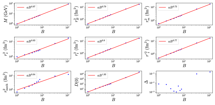
Figure 1: Dependence of various quantities on the baryon number. We also plot the mass $M$ and $\Delta$ as defined in (25).

IV Numerical results

We use the original Skyrme model Lagrangian supplemented with the pion mass term. Its precise form as well as our numerical approach is explained in Garcia Martin-Caro et al. (2023) to which we refer the reader. In order to numerically confirm relations such as (11) which are sensitive to the difference of radii, we need more accurate solutions than those presented in Garcia Martin-Caro et al. (2023). This has been achieved by enlarging the 3D grid (up to $N^{3}=(151)^{3}$ points) and accelerating the energy-minimization process via a parallelization of the numerical algorithm using the OpenMP C++ package. Thanks to this improvement, the error

$$\Delta=\absolutevalue{\frac{\langle r^{2}\rangle_{m}-\langle r^{2}\rangle_{s}}{\frac{3D(0)}{M^{2}}}-1}$$ (25)

is less than 1% for the solutions $1\leq B\leq 8$. (But we still have $\Delta\sim 10\%$ for the $B=32,108$ solutions.) We have then fixed the parameters of the model (see Eq. (1) of Garcia Martin-Caro et al. (2023)) as $f_{\pi}=117.23\operatorname{MeV},$ $e=4.81$ and $m_{\pi}=138\operatorname{MeV}$ such that the proton’s mass $M=0.938$ GeV and charge radius $\sqrt{\langle r^{2}\rangle_{c}}=0.84$ fm are reproduced. The sextic coupling discussed in Garcia Martin-Caro et al. (2023) has been turned off. Below we introduce a simpler notation for the root mean square radii $\sqrt{\langle r^{2}\rangle_{m}}\equiv r_{m}$, etc. In Fig. 1, we plot the radii $r_{m}$, $r_{s}$, $r_{t}$, $r_{mech}$ and $r_{B}$ as a function of $B$, including $r^{\prime}_{t}$ (12) for completeness. The actual values are complied in Table 1 together with the masses $M$ and the values of $D(0)$ (revised from Garcia Martin-Caro et al. (2023) due to different parameters). We confirm the expected ordering $r_{t}<r_{m}<r_{s}$. Curiously, $r_{t}$ and $r_{B}$ agree within less than 2%. From these results, we have extracted the exponent

$$r_{m}\sim B^{0.37},\quad r_{s}\sim B^{0.32},\quad r_{t}\sim B^{0.4},\quad r_{B}\sim B^{0.4},\quad r_{mech}\sim B^{0.32}.$$ (26)

These are roughly consistent with the usual formula $r\sim B^{1/3}$, but there are systematic deviations. In particular, $r_{mech}$ may not be characterized by a simple power-law distribution (see the bottom-left plot in Fig. 1). It is also interesting to notice that $r_{t}$ grows faster with $B$ than $r_{m}$ which in turn grows faster than $r_{s}$. As a result, $r_{t}$, $r_{m}$ and $r_{s}$ converge as $B$ is increased. Indeed, the difference between any two of them behaves as

$$\frac{D(0)}{M^{2}}\propto B^{\beta-2},$$ (27)

with $\beta\approx 1.92$. Thus the differences go to zero as $B\to\infty$. A similar behavior is expected for the model of Liuti and Taneja (2005) which predicted $\beta\approx 1$. In contrast, the differences increase with $B$ in the models of Polyakov (2003); Guzey and Siddikov (2006) where $\beta\approx 2.3$.

$B$	$M$ (GeV)	$r_{B}$	$r_{m}$	$r_{s}$	$r_{t}$	$r^{\prime}_{t}$	$r_{\rm mech}$	$D(0)$	$p(0)$ (GeV/fm3)
1	0.938	0.642	0.778	1.002	0.638	0.688	0.817	-2.98	0.3465
2	1.795	0.876	0.966	1.149	0.861	0.898	1.106	-10.61	-0.0362
3	2.616	1.022	1.094	1.251	1.006	1.036	1.291	-21.62	-0.0203
4	3.408	1.138	1.197	1.335	1.121	1.147	1.448	-34.78	-0.0173
5	4.254	1.269	1.32	1.439	1.256	1.278	1.661	-50.92	-0.0185
6	5.064	1.376	1.42	1.525	1.364	1.383	1.862	-68.25	-0.0196
7	5.845	1.433	1.47	1.568	1.418	1.436	1.993	-87.24	-0.0173
8	6.698	1.533	1.566	1.651	1.521	1.536	2.305	-105.31	-0.0183
32	26.436	2.642	2.680	2.744	2.648	2.659	3.055	-1859.08	0.0000
108	88.311	4.077	4.114	4.165	4.088	4.097	3.499	-24151.55	-0.0171

Table 1: Root mean square radii of Skyrmions in units of $\operatorname{fm}$. The proton charge radius $r_{c}=0.84$ fm is used as an input.

In Fig. 2, we plot the ‘pressure’ distribution $p(r)$ (left) and $r^{2}p(r)$ (right). We numerically checked consistency between the two definitions (22) and (24). Remarkably, we find that $p(0)$ is negative for all the solutions with $B>1$ except for $B=32$ where $p(0)$ is consistent with zero up to ${\cal O}(10^{-6})$. Actually, the same phenomenon has been recently found in He and Zahed (2023) for the $B=4$ nucleus (helium-4) with one particular choice of the nuclear wavefunction, but not for the deuteron ($B=2$). This is at first sight surprising and even unlikely because, from (22),

$$p(0)=\frac{-1}{24\pi^{2}M}\int_{-\infty}^{0}dt(-t)^{\frac{3}{2}}D(t).$$ (28)

If $D(t)$ is negative definite, clearly $p(0)$ is positive. However, as already observed in Garcia Martin-Caro et al. (2023), $D(t)$ turns positive in the large-$|t|$ region for the $B>1$ solutions, and due to the weight factor $(-t)^{\frac{3}{2}}$, this region dominates the integral in practice. A more intuitive way to understand this phenomenon is to notice that the solutions with $B>1$ have a ‘hollow’ in the core region where the energy density is lower than in the surrounding region . This results in an inward flux near the origin which may be interpreted as negative pressure. For light nuclei $2\leq B\leq 8$, $p(r)$ then turns positive in the intermediate $r$-region and becomes negative again at large-$r$. Pressure per solid angle $r^{2}p(r)$ has a stronger peak at an increasingly large value of $r$ as $B$ is increased. In the case of large nuclei $B=32,108$, $p(r)$ shows a striking oscillating pattern, similar to the oscillation of $D(t)$ found in Garcia Martin-Caro et al. (2023). This is probably due to the fact that, in the present model, these nuclei are realized as an ‘$\alpha$-cluster’, an organized spatial arrangement of $B=4$ solutions, see Fig. 1 of Garcia Martin-Caro et al. (2023). The energy density also oscillates as a function of $r$.

A common interpretation of the $p(r)$ curve of the nucleon (see the $B=1$ curve in Fig. 2) is that the ‘confining’ force $p(r)<0$ in the outer region is counteracted by the ‘repulsive core’ $p(r)>0$ near the origin Goeke et al. (2007); Cebulla et al. (2007); Burkert et al. (2018); Lorcé et al. (2019). This provides an appealing scenario of how the nucleon may be stabilized. However, such an interpretation does not hold verbatim for $B>1$ nuclei especially when $B\gg 1$, suggesting that the mechanical stability argument for nuclei is more nontrivial. One should also keep in mind that the ‘pressure’ (22) defined by the $D(t)$-form factor is not genuine thermodynamic pressure. The existence of negative regions $p<0$ is a reminder of this caveat.

In order to see the nature of (22) and its limitation from a different perspective, let us naively assume the standard thermodynamical relation between the pressure, baryon number (16) and energy $\varepsilon=T^{0}_{0}$ densities of a zero-temperature, barotropic fluid Danielewicz et al. (2002)

$$p(\rho_{B})=\rho_{B}^{2}\partialderivative{(\varepsilon/\rho_{B})}{\rho_{B}}.$$ (29)

Assuming spherical symmetry, one could write an alternative expression for $p(r)$

$$p(r)=\frac{\rho_{B}(r)}{\rho_{B}^{\prime}(r)}\varepsilon^{\prime}(r)-\varepsilon(r).$$ (30)

This is plotted in Fig. 3 (left) together with (22) for $B=1$. It can be seen that the two definitions of pressure do not coincide. This is not surprising, as the energy and baryon number densities have been computed independently of each other, and a priori there is no reason why (30) should coincide with (22). (We are however surprised that the two curves are rather close.) Note also that (29) asserts that the on-shell Skyrmion configurations satisfy the barotropic equation of state $p=p(\rho_{B})$, which has been argued to not be the case for Skyrmion solutions in the context of the equation of state of neutron stars Adam et al. (2015). For non-spherical Skyrmions with $B>1$, we may define $\rho_{B}(r)$ and $\varepsilon(r)$ by averaging over the solid angles. However, (30) is hard to compute numerically in practice because for $B>1$ the radial derivatives vanish at some finite value of $r$, and only an exact cancellation of the zeros yields a finite result. Away from this point, the two definitions are seen to disagree as in Fig. 3 (right) in the case of $B=2$.

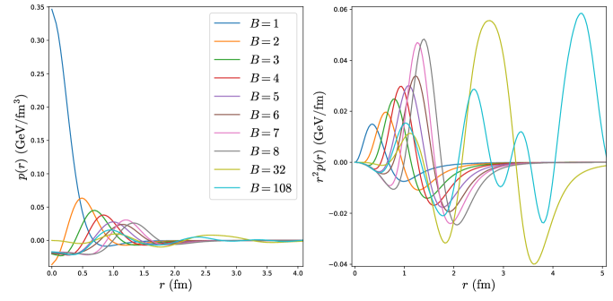
Figure 2: Effective radial pressure density for Skyrmions with $B=1\sim 8$.

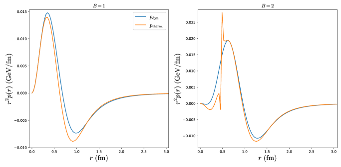
Figure 3: Pressure defined by (30) (orange) and by (22) (blue) for the $B=1$ (left) and $B=2$ (right) solutions. In the right panel, numerical accuracy is lost for $r\lesssim 0.6\operatorname{fm}$ due to the error induced by the non-exact cancelation of vanishing radial derivatives in (30). Still, appreciable differences between both pressure definitions appear for larger values of the radius.

V Conclusions

In conclusion, we have computed various definitions of radius for a variety of nuclei in the Skyrme model and studied their $B$-dependence. Their relations to the D-term have been numerically confirmed to good precision. These radii are associated with different components of the energy momentum tensor and have different physical interpretations. Together with the more familiar charge radius, they characterize the rich internal structure of the nucleon and nuclei. We have also computed the ‘pressure’ distribution and found that $p(r)$ is negative in the core region of all the $B>1$ nuclei explored in this work. This is due to the sign change of the $D(t)$ form factor at large $|t|$, and is presumably related to the ‘hollowness’ of the $B>1$ Skyrmions. Whether this is a general feature or an artifact of the model is unclear to us. It is therefore worthwhile to compute the present observables in more realistic approaches using the machinery of low energy nuclear physics.

A final remark concerning the semi-classical approximation adopted in this work is in order. It is well known that the energy momentum tensor components get quantum corrections at first order in the $N_{c}^{-1}$ expansion due to the spin and isospin degrees of freedom. Thus, a natural extension of the work presented here would be to study how the different radii and their $B$-dependences get affected by such corrections. While we do not expect large differences from what we have predicted here just by using the classical solutions, it is still interesting to study how the energy and pressure distributions differ between isobaric nuclei, as is the case with the charge density Danielewicz and Lee (2014).

References

- Hofstadter (1956) R. Hofstadter, Rev. Mod. Phys. 28, 214 (1956).
- Frosch et al. (1968) R. F. Frosch, R. Hofstadter, J. S. McCarthy, G. K. Noldeke, K. J. van Oostrum, M. R. Yearian, B. C. Clark, R. Herman, and D. G. Ravenhall, Phys. Rev. 174, 1380 (1968).
- De Vries et al. (1987) H. De Vries, C. W. De Jager, and C. De Vries, Atom. Data Nucl. Data Tabl. 36, 495 (1987).
- Sick (2008) I. Sick, Phys. Rev. C 77, 041302 (2008).
- Carlson (2015) C. E. Carlson, Prog. Part. Nucl. Phys. 82, 59 (2015), arXiv:1502.05314 [hep-ph] .
- Gao and Vanderhaeghen (2022) H. Gao and M. Vanderhaeghen, Rev. Mod. Phys. 94, 015002 (2022), arXiv:2105.00571 [hep-ph] .
- Pohl et al. (2010) R. Pohl et al., Nature 466, 213 (2010).
- Xiong et al. (2019) W. Xiong et al., Nature 575, 147 (2019).
- Krauth et al. (2021) J. J. Krauth et al., Nature 589, 527 (2021).
- Kopecky et al. (1995) S. Kopecky, P. Riehs, J. A. Harvey, and N. W. Hill, Phys. Rev. Lett. 74, 2427 (1995).
- Kobzarev and (1962) I. Y. Kobzarev and L. B. , Zh. Eksp. Teor. Fiz. 43, 1904 (1962).
- Pagels (1966) H. Pagels, Phys. Rev. 144, 1250 (1966).
- Goeke et al. (2007) K. Goeke, J. Grabis, J. Ossmann, M. V. Polyakov, P. Schweitzer, A. Silva, and D. Urbano, Phys. Rev. D 75, 094021 (2007), arXiv:hep-ph/0702030 .
- Cebulla et al. (2007) C. Cebulla, K. Goeke, J. Ossmann, and P. Schweitzer, Nucl. Phys. A 794, 87 (2007), arXiv:hep-ph/0703025 .
- Kumano et al. (2018) S. Kumano, Q.-T. Song, and O. V. Teryaev, Phys. Rev. D 97, 014020 (2018), arXiv:1711.08088 [hep-ph] .
- Burkert et al. (2018) V. D. Burkert, L. Elouadrhiri, and F. X. Girod, Nature 557, 396 (2018).
- Hatta and Yang (2018) Y. Hatta and D.-L. Yang, Phys. Rev. D 98, 074003 (2018), arXiv:1808.02163 [hep-ph] .
- Mamo and Zahed (2020) K. A. Mamo and I. Zahed, Phys. Rev. D 101, 086003 (2020), arXiv:1910.04707 [hep-ph] .
- Kharzeev (2021) D. E. Kharzeev, Phys. Rev. D 104, 054015 (2021), arXiv:2102.00110 [hep-ph] .
- Sun et al. (2021) P. Sun, X.-B. Tong, and F. Yuan, Phys. Lett. B 822, 136655 (2021), arXiv:2103.12047 [hep-ph] .
- Duran et al. (2023) B. Duran et al., Nature 615, 813 (2023), arXiv:2207.05212 [nucl-ex] .
- Wang et al. (2022) X.-Y. Wang, F. Zeng, and Q. Wang, Phys. Rev. D 105, 096033 (2022), arXiv:2204.07294 [hep-ph] .
- Guo et al. (2023) Y. Guo, X. Ji, Y. Liu, and J. Yang, Phys. Rev. D 108, 034003 (2023), arXiv:2305.06992 [hep-ph] .
- Wang et al. (2023) R. Wang, C. Han, and X. Chen, (2023), arXiv:2309.01416 [hep-ph] .
- Adhikari et al. (2023) S. Adhikari et al. (GlueX), Phys. Rev. C 108, 025201 (2023), arXiv:2304.03845 [nucl-ex] .
- Hatta (2023) Y. Hatta, (2023), arXiv:2311.14470 [hep-ph] .
- Abdul Khalek et al. (2022) R. Abdul Khalek et al., Nucl. Phys. A 1026, 122447 (2022), arXiv:2103.05419 [physics.ins-det] .
- Garcia Martin-Caro et al. (2023) A. Garcia Martin-Caro, M. Huidobro, and Y. Hatta, Phys. Rev. D 108, 034014 (2023), arXiv:2304.05994 [nucl-th] .
- Skyrme (1961) T. H. R. Skyrme, Proc. Roy. Soc. Lond. A 260, 127 (1961).
- Polyakov (2003) M. V. Polyakov, Phys. Lett. B 555, 57 (2003), arXiv:hep-ph/0210165 .
- Liuti and Taneja (2005) S. Liuti and S. K. Taneja, Phys. Rev. C 72, 034902 (2005), arXiv:hep-ph/0504027 .
- Guzey and Siddikov (2006) V. Guzey and M. Siddikov, J. Phys. G 32, 251 (2006), arXiv:hep-ph/0509158 .
- He and Zahed (2023) F. He and I. Zahed, (2023), arXiv:2310.12315 [nucl-th] .
- Fujita et al. (2022) M. Fujita, Y. Hatta, S. Sugimoto, and T. Ueda, PTEP 2022, 093B06 (2022), arXiv:2206.06578 [hep-th] .
- Ji (2021) X. Ji, Front. Phys. (Beijing) 16, 64601 (2021), arXiv:2102.07830 [hep-ph] .
- Mamo and Zahed (2022) K. A. Mamo and I. Zahed, Phys. Rev. D 106, 086004 (2022), arXiv:2204.08857 [hep-ph] .
- Polyakov and Schweitzer (2018) M. V. Polyakov and P. Schweitzer, Int. J. Mod. Phys. A 33, 1830025 (2018), arXiv:1805.06596 [hep-ph] .
- Feist et al. (2013) D. T. J. Feist, P. H. C. Lau, and N. S. Manton, Phys. Rev. D 87, 085034 (2013), arXiv:1210.1712 [hep-th] .
- Gudnason and Halcrow (2018) S. B. Gudnason and C. Halcrow, Phys. Rev. D 98, 125010 (2018), arXiv:1811.00562 [hep-th] .
- García Martín-Caro and Halcrow (2023) A. García Martín-Caro and C. Halcrow, (2023), arXiv:2312.04335 [nucl-th] .
- Halcrow (2023) C. Halcrow, “Skyrmions3D,” https://github.com/chrishalcrow/Skyrmions3D.jl (2023).
- Braaten and Carson (1989) E. Braaten and L. Carson, Phys. Rev. D 39, 838 (1989).
- Carson (1991) L. Carson, Nucl. Phys. A 535, 479 (1991).
- Gillard et al. (2015) M. Gillard, D. Harland, and M. Speight, Nucl. Phys. B 895, 272 (2015), arXiv:1501.05455 [hep-th] .
- Gudnason (2018) S. B. Gudnason, Phys. Rev. D 98, 096018 (2018), arXiv:1805.10898 [hep-ph] .
- Lorcé et al. (2019) C. Lorcé, H. Moutarde, and A. P. Trawiński, Eur. Phys. J. C 79, 89 (2019), arXiv:1810.09837 [hep-ph] .
- Danielewicz et al. (2002) P. Danielewicz, R. Lacey, and W. G. Lynch, Science 298, 1592 (2002), arXiv:nucl-th/0208016 .
- Adam et al. (2015) C. Adam, T. Klähn, C. Naya, J. Sanchez-Guillen, R. Vazquez, and A. Wereszczynski, Phys. Rev. D 91, 125037 (2015), arXiv:1504.05185 [hep-th] .
- Danielewicz and Lee (2014) P. Danielewicz and J. Lee, Nucl. Phys. A 922, 1 (2014), arXiv:1307.4130 [nucl-th] .