Nanoparticle Interferometer by Throw and Catch

Abstract

Matter-wave interferometry with increasingly larger masses could pave the way to understanding the nature of wavefunction collapse, the quantum to classical transition or even how an object in a spatial superposition interacts with its gravitational field. In order to improve upon the current mass record, it is necessary to move into the nano-particle regime. In this paper we provide a design for a nano-particle Talbot-Lau matter-wave interferometer that circumvents the practical challenges of previously proposed designs. We present simulations of the expected fringe patterns that such an interferometer would produce, considering all major sources of decoherence. We discuss the practical challenges involved in building such an experiment as well as some preliminary experimental results to illustrate the proposed measurement scheme. We show that such a design is suitable for seeing interference fringes with $10^{6}$ amu SiO₂ particles, and that this design can be extended to even $10^{8}$ amu particles by using flight times below the typical Talbot time of the system.

I Introduction

Interferometry techniques have historically been the most popular method for demonstrating wave-like behaviour. Perhaps the most famous example of this was Young’s double slit experiment, performed in 1801, which demonstrated the wave nature of light [1]. The subsequent works of Planck and Einstein showed that light also possesses particle like features in the form of photons. The idea of wave-particle duality, extended to also encompass matter, was then famously formalised by Louis de Broglie in his 1924 Ph.D. thesis where he claimed electrons could also behave like waves with their wavelength being dependant on their momentum [2]. His prediction was later verified by Davisson and Germer in 1927 who, like Young, performed a double slit experiment to show interference in electrons [3].

Since wave-particle duality is a core tenant of quantum mechanics, testing this phenomenon at increasingly larger scales could give us some much-needed insight into poorly understood areas of quantum mechanics such as the nature of wave function collapse, the so called ‘measurement problem’, or how massive quantum objects interact with their gravitational fields. A lot of progress has been made in the field of matter-wave interferometry since the electron double slit experiment, initially with atoms of increasing mass [4], and then with larger and larger macro-molecules. The current mass record for observing matter-wave interference is held by Markus Arndt’s group in Vienna who used a Talbot Lau Interferometer (TLI) scheme to demonstrate matter-wave interference of molecules of masses up to 25,000 atomic mass units (amu) [5].

These near-field techniques were pioneered by Clauser and Li [6], who demonstrated the Talbot Lau interferometry in atoms before the rise of cold atomic ensemble experiments enabled by laser cooling techniques. Famously extending matter-wave interferometry to higher masses in 1999 where the interference patterns of buckminsterfullerene (C₆₀) were shown [7] in the far-field and shortly later in molecular TLI scheme as well [8].

Further probing of the fundamentals of quantum mechanics will require larger mass matter-wave interferometric experiments. However, the molecular techniques used in these experiments have inherent problems with scaling up to ever larger masses. Especially challenging is the provision of coherent particle beam sources, given there are limited capabilities for cooling the center of mass motion of large molecules and clusters [9]. For this reason, in this paper we aim to introduce a new scheme for the detection of interference effects using SiO₂ nanoparticles using a ‘throw and catch’ design. Silica nanoparticles have large polarisabilities, which opens the opportunity for manipulation and indeed cooling to the motional ground state by optical techniques beside others in the emerging field of levitated mechanics [10]. The interferometer approach will be heavily based on the proposal suggested by Bateman et al. in 2014 [11], with the throw and catch scheme intended to alleviate practical issues of the original proposal, such as inefficient reloading. We will show the expected interference patterns produced whilst using realistic experimental parameters for both $10^{6}$ amu and $10^{8}$ amu particles including all major sources of decoherence.

II Experimental Set-Up

The key idea behind this proposal is to use the core concepts presented in Bateman et al. whilst implementing a method of reusing the same particle throughout the generation of the interference pattern. This will alleviate practical issues of loading and re-using nanoparticles since re-trapping an appropriate particle can take hours. It will also give us a completely identical source for each run of the experiment, thereby reducing decoherence effects from non-identical sources. This is demonstrated in appendix A figure A0.

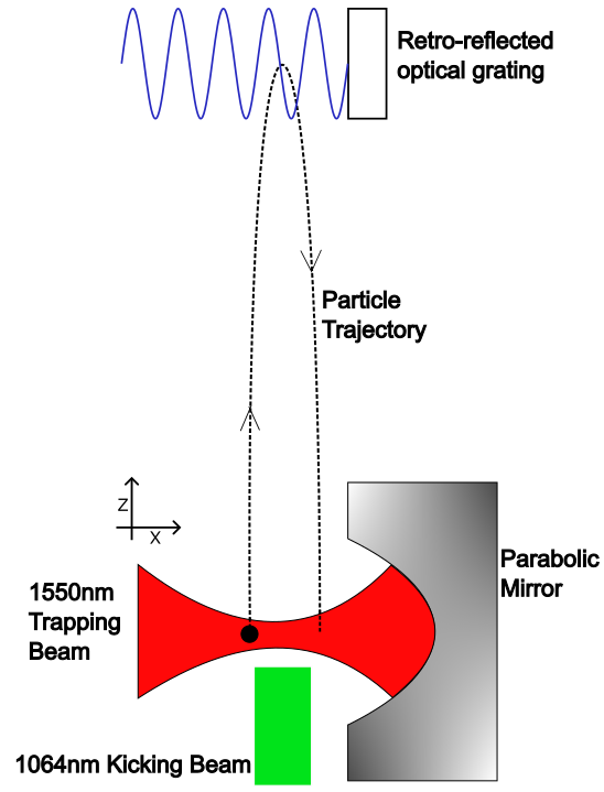
Figure 1: Schematic of the proposed experimental set-up. The particle is shown as being kicked when not exactly at the trapping center to demonstrate the generally parabolic trajectory.

A rough outline of the scheme is shown in Figure 1. We begin with trapping a silicon dioxide nanosphere using a parabolic trap detailed in [12]. We use a 1550nm laser with an incident power of approximately 100mW for the purposes of trapping using the standard optical tweezer technique. The light scattered by the particle will be collimated by the parabola and detected to track the particle motion. The particle behaves as a simple harmonic oscillator and its motion modulates the phase of the trapping laser beam. By interfering the scattered light with the light that misses the particle we can extract this phase information and identify the particles modes of motion. We then use this information to implement feedback cooling, via a lock in amplifier which modulates the trapping light, to decrease the motional temperature of the particle to approximately 1mK along the direction of the later grating. This results in a momentum uncertainty $\sigma_{p}/m$ of less than $0.1$cms^-1 and a positional uncertainty of less than $1$nm for a $10^{8}$amu particle. The particle in our trap hence acts as a coherent source of matter-waves.

After the cooling we turn-off the trapping light and apply a vertical impulsive force via the action of a 1064nm laser pulse. The power of the laser is tuned to achieve the required flight time to generate, via the Talbot effect, an experimentally detectable quantum interference pattern. The Talbot effect is a near field interference effect where the image of the diffraction grating, that a wave passes through, is repeated at regular intervals. The distance between these intervals is known as the Talbot length and by knowing the velocity of our particle we can also think of this as a Talbot time. In order to be confident of seeing such an interference pattern, the flight time of our particle ought to be on the scale of the Talbot time, which is around $2.8$s, for the case of a $10^{8}$amu particle. However, we will show that this is not such a strict requirement. Halfway through the particles total flight time, at the peak of its trajectory, a secondary laser pulse of wavelength $213$nm, and nanosecond duration, is imparted onto the particle. This pulse is retro-reflected by a mirror in order to form an optical grating through which the matter-wave is diffracted. This process introduces a position dependant phase shift to the wave function of the matter-wave hence forming the basis for our interference pattern.

The final stage for our proposed interferometer is the measurement and ‘catch’. The optical trap is turned back on once the particle is just above the height it started at in order to slow down and recapture it. Precise timing will be important here since, if the trap is turned on too early the initial re-entry will accelerate the particle so much so that it will be fall out of the trap. This will be explained in more detail below. Once the particle is recaptured, we will once again be able to track its position as discussed earlier. By extrapolating this information back to the time at which the particle entered the trapping centre we can measure the position it landed at as demonstrated in Hebestreit et al. in 2018 [13]. We will require roughly a $10$nm precision in order to detect our interference patterns. Initial testing shows that this should be achievable even with rudimentary data extraction techniques, with work ongoing on more advanced methods. The particle is then re-cooled and prepared to its initial state as described above, which only requires a few trapping cycles, and hence does not introduce major heating effects. Over many runs a probability distribution of particle arrival locations is produced which can be compared to the expected classical ballistic and quantum wave-like patterns discussed in the following.

III Theoretical Model

III.1 Background

As mentioned before, the design of the throw and catch experiment maintains the core aspects of the proposal set out in Bateman et al. [11]. This allows us to work with the existing theory presented in Bateman et al. and later built upon in Belenchia et al. [14]. The only differences which need to be considered for the throw and catch variant are some additional decoherence effects which will be discussed shortly. For this reason we only give a brief overview of the theoretical background here, deferring to the aforementioned publications for a more detailed description.

We begin our experiment with the nano-particle trapped by our $1550$nm optical trap and behaving as a harmonic oscillator. This state is well described as a Gaussian thermal state of motion with standard deviations in position and momentum given by $\sigma_{x}=\sqrt{k_{B}T/4\pi^{2}m\nu^{2}_{M}}$ and $\sigma_{p}=\sqrt{mk_{B}T}$ respectively. Here $T$ is the motional temperature of the oscillator, $m$ is the mass of our particle and $\nu_{M}$ is the trap frequency as defined from the standard harmonic oscillator relationship between restoring force and position. At this point it is important to note that since our grating is a uniform standing wave oriented along the $x$-axis, as shown in Figure 1. Assuming the laser waist in the $y$ direction is large enough and that the overall $y$ displacement is small throughout the journey, the grating should have a negligible impact on the evolution of the state in the $y$ and $z$ directions. This allows us to effectively neglect these directions when evaluating our final interference pattern since this pattern will only exist along the $x$ direction. This is a crucial similarity between our work here and the preceding work in Bateman et al. [11].

We begin with the free evolution of the particle, after the kick, up to its peak. This occurs in a time $t_{1}$. Then the interaction with the grating, followed by another period of free evolution as the particle falls back down into the trap where its position is finally measured. This second period of free evolution occurs in a time $t_{2}$ and in our case $t_{1}=t_{2}$. We assume the kick procedure can be modeled as a positive shift of the vertical velocity distribution of the particle state. Under this assumption we can use the expression derived in [11] to describe the final probability density function, upon measurement, that is:

$$w(x) =\frac{m}{\sqrt{2\pi}\sigma_{p}\left(t_{1}+t_{2}\right)}\sum_{n}B_{n}\left[\frac{nt_{1}t_{2}}{t_{\mathrm{T}}\left(t_{1}+t_{2}\right)}\right]$$ (1)

$$\times\exp\left[\frac{2\pi inx}{D}-\frac{2\pi^{2}n^{2}\sigma_{x}^{2}t_{2}^{2}}{d^{2}\left(t_{1}+t_{2}\right)^{2}}\right].$$

This expression is of the form of a periodic fringe pattern oscillating at the period $D=d(t_{1}+t_{2})/t_{1}$, with $d$ being the grating spacing given by $\lambda_{G}=2d$. $t_{T}$ in the above expression is the Talbot time given by $t_{T}=md^{2}/h$ which sets the time scale that our nanosphere wave packet needs to evolve for in order to reasonably expect to see a near field interference pattern. Finally, the $B_{n}$ terms are the so-called Talbot coefficients which characterize the general shape of the interference pattern. For nanoparticles in the Rayleigh limit, that is whose linear dimension is sufficiently smaller than the grating period, these coefficients take the form

$$B_{n}(y)=J_{n}(\phi_{0}\sin(\pi y)),$$ (2)

where $J_{n}$ denotes a Bessel function of the first kind. The $\phi_{0}$ in the above expression is referred to as the phase modulation parameter and comes from the expression for the effect that the optical grating has on the particle’s wave-function. In the longitudinal eikonal approximation, and ignoring incoherent effects, the quantum state evolves as:

$$\langle x|\psi\rangle\rightarrow\exp\left(i\phi_{0}\cos^{2}\left(\frac{\pi x}{d}\right)\right)\langle x|\psi\rangle,$$ (3)

where

$$\phi_{0}=\frac{2\operatorname{Re}(\alpha)E_{G}}{\hbar c\epsilon_{0}a_{G}}.$$ (4)

Here $\alpha$ denotes the particle’s optical polarizability, whilst $E_{G}$ and $a_{G}$ are the energy and spot size of the optical grating pulse respectively.

It should be noted that also classical particles traversing the optical grating, and moving on ballistic trajectories, give rise to a shadow fringe pattern [15, 11, 14]. This classical pattern, in the Rayleigh limit, is described by the same expression as in Eq. (1) but with $\sin(\pi y)\rightarrow\pi y$ in Eq. (2). In order to claim the observation of quantum fringes, it is thus crucial to be able to distinguish the quantum fringe pattern from this classical shadow. For the case of finite-size particles we refer the reader to the derivation in [14].

III.2 Accounting for decoherence and particle size

The background theory presented above is a good foundation for understanding the quantum behaviour of our proposed experiment in the absence of decoherence. Nonetheless in order to determine the viability of seeing interference fringes in the lab we must account for all major sources of decoherence that will reduce the visibility of our fringes. We begin by describing the effects of decoherence events that have already been accounted for in previous works. These include collisions with residual gas particles, scattering and absorption of black-body photons, and thermal emission of radiation. The way these enter into our predicted interference pattern is by multiplying each Talbot coefficient, described in Eq. (2), by a reduction factor of the form

$$R_{n}=\exp\left\{-\Gamma\left[1-f\left(\frac{nht_{2}}{mD}\right)\right]\left(t_{1}+t_{2}\right)\right\},$$ (5)

which wash out our expected interference fringes. $\Gamma$ here gives the rate of decoherence events whilst $f(x)$ denotes their spatial resolution.

With these decoherence events accounted for it is now time to consider the fact that our particle is not point-like, which is an assumption that has been implicitly made throughout the theory presented thus far. Relaxing this assumption has two major implications, it will change the form of the phase modulation parameter $\phi_{0}$ introduced in Eq. (4), and impact the form of the reduction factors for scattering decoherence events that we are yet to account for. The point-like particle assumption is well justified in the Rayleigh scattering regime, that is when the radius of the particle is small compared to the wavelength of our optical grating, $kR<<1$, with $k$ being the standard wave-number given by $k=2\pi/\lambda_{G}$. This will be mostly satisfied for the simulation work presented here, however, our ambitions are to attempt performing this experiment for increasingly larger particles that are very close in size to the wavelength of the grating we intend to use. For a $10^{8}$ amu particle, $kR$ is already as high as $0.83$. This means we must work in the Mie scattering regime instead. In this regime the form of the phase modulation parameter is adjusted to [14]

$$\phi_{0}=\frac{8F_{0}E_{G}}{\hbar c\epsilon_{0}a_{G}k|E_{0}|^{2}},$$ (6)

where $E_{0}$ is the amplitude of our standing wave grating and $F_{0}$ is the force exerted on our particle, modeled by a dielectric sphere, by the grating according to Mie scattering theory. The expression for $F_{0}$ is long and not particularly enlightening, we thus refer the reader to [14] for a detailed derivation and discussion. The key takeaway here is that whilst the Rayleigh approximation predicts an exponential increase in $\phi_{0}$ with particle size, the Mie scattering correction predicts a steep sinusoidal fall-off in $\phi_{0}$ around the point $kR=1$. Since this phase modulation parameter is exactly what ends up being converted into our spatial interference fringes, it is imperative that we avoid these regions of low $\phi_{0}$ when dealing with larger particles. Finally we must also consider decoherence from the incoherent part of the scattering process and from absorption of grating photons. These fundamentally enter the expression for the interference pattern in the same way as the decoherence effects we have already discussed but with more complicated versions of $R_{n}$. For a full treatment of these terms we once again refer to Belenchia et al. [14], see however [16] and appendix B for a correction to Eq.(28) of [14]. In the following, we include all these incoherent and coherent effects, treated in the full Mie scattering theory, in our simulations. Note we could also consider the misalignment of the grating relative to the particle’s trajectory however, this only leads to a net shift of the interference fringes and does not lead to a loss of visibility. This is discussed in the supplementary material of Bateman et al. [11] and will not be considered further here.

We now discuss a novel decoherence source specifically associated with the throw and catch scheme. This is the degree to which we are able to control the energy of the kicking laser pulse. An error in the kicking laser energy will cause an error in the flight time of the particle. If this error varies randomly over many runs that together build up our interference pattern, then this will lead to a smearing out of fringes as with other sources of decoherence. Unlike the other sources of decoherence mentioned earlier, this one is modelled by simulating many interference patterns, with normally distributed flight times that would be expected for an imperfect kicking laser, and then averaged to create the final expected interference pattern. As with the requirement on cooling, we will see that the practical restriction of being able to recapture the particle is a stricter condition than what is needed to manage the decoherence effect coming from this error.

IV Practical Considerations

Firstly, it is important to mention the steps we expect to take to minimise the effects of decoherence to manageable levels. We minimise decoherence due to thermal emission of black body photons by minimising the rate of absorption, and therefore the rate of heating, of the particle whilst it is in the trap. Our silica particles have a particularly low absorption cross section for the $1550$nm light which we are using to trap them. Decoherence by collisions with background gas particles is minimised by working at ultra-high-vacuum ($10^{-10}$ mbar). Scattering and absorption decoherence at the grating laser is minimised by using a short ($5$ns) pulse to limit the interaction time.

With this in mind we now discuss how practical restrictions on our ability to recapture the particle may end up being more restrictive on our potential interference pattern than any of the discussed decoherence events. Before we proceed, it is important to note that the strict cooling requirements that we discuss here could potentially be circumvented by tracking the particle and selecting to kick it only when it is in a low velocity region of its oscillation. Whilst we won’t discuss selection in more detail here, this is also an area of active investigation. In the following section we will present the conditions needed to achieve an interferometer height of $10$cm, this height is roughly what would be required to achieve flight times on the order of the Talbot time for a $10^{6}$amu particle.

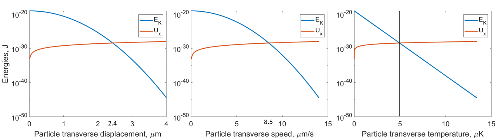
Figure 2: Matching point of optical potential energy barrier and particle kinetic energy. (a) The particle’s transverse displacement must be less than 2.4$\mu$m for it to be re-captured. (b) To achieve that transverse displacement during the total flight time of $285.6$ms, to and from a height of 10 cm, the transverse speed must be less than 8.5 $\mu$ms^-1. (c) That speed corresponds to a temperature of the oscillation along $x$ of less than 5$\mu$K.

We can begin to understand the cooling conditions on re-capture by noticing that when the particle is pushed vertically by the radiation pressure of the laser pulse, it will also have a transverse velocity $v_{x}$. To recapture the returning particle, it must enter the optical trap at a transverse position where the optical potential barrier is greater than the transverse kinetic energy of the particle. This transverse velocity is a measure of the particle’s transverse temperature before release. The optical potential energy barrier posed by the gradient force has the form [17]:

$$U_{x}=\frac{\operatorname{Re}(\alpha)}{2c\epsilon_{0}}I(x),$$ (7)

where $\alpha$ is the electric polarizability of the particle and $I(x)$ is the intensity distribution of the laser along the $x$ direction. We impose the constraint that when the particle reaches the focal plane ($z=0$), its kinetic energy is equal to that of the optical potential barrier. The intensity distribution, assumed to be Gaussian, along $x$ is then:

$$I(x,0,0)=\frac{2P}{\pi w_{0}^{2}}\exp\left[-2\left(\frac{x}{w_{0}}\right)^{2}\right],$$ (8)

where $w_{0}$ is the laser waist in the focus of the parabola and $P$ is the power contained within the waist. The potential energy as a function of $x$ becomes:

$$U_{x}=\frac{\operatorname{Re}(\alpha)P}{c\epsilon_{0}\pi w_{0}^{2}}\exp\left[-2\left(\frac{x}{w_{0}}\right)^{2}\right].$$ (9)

$x$ can also be written as a function of the (constant) radial velocity, $v_{x}$:

$$x=2v_{x}t=2v_{x}\cdot\sqrt{2h/g},$$ (10)

where $t=\sqrt{2h/g}$ is the time needed for the particle to free fall from height $h$ and the $2$ multiplication comes from the fact that the particle travels sideways at $v_{x}$ during both the up and down motion along $z$. Equating this:

$$\frac{mv_{x}^{2}}{2}=\frac{\operatorname{Re}(\alpha)P}{c\epsilon_{0}\pi w_{0}^{2}}\exp\left[-2\left(\frac{x}{w_{0}}\right)^{2}\right].$$ (11)

Graphically solving the above equation, we can then determine the cooling constraint on the maximal initial transverse displacement, initial transverse speed and the corresponding temperature compatible with a throw and catch scheme with a height of 10cm. In figure 2(c), we can see that the temperature of the oscillator must be less than 5$\mu$K. The ground state temperature of our nanoparticle, when oscillating at $50$kHz, is $2.2\mu$K, and cooling down to this temperature has been achieved [18]. This means that the cooling requirements for a $10$cm height throw and catch are close to the cutting edge, but achievable.

We also note that a lower frequency means larger displacement at the same temperature:

$$x_{rms}=\sqrt{\frac{k_{B}T}{m\omega_{0}^{2}}}$$ (12)

Since particle displacement is what we are detecting, it may be easier to detect this more ample motion at a lower frequency than a less ample motion at a higher frequency. A lower oscillation frequency would require less power, which reduces the heating and re-emission rate of the particle. These have been pointed out as problematic in [11].

Now, turning our attention to the $z$ direction, the following can be said. If the particle is launched vertically at around $1$ms^-1, then we can expect the same speed as it returns. The challenge now is to restart the laser at the right time in order to catch and re-cool the particle. The trapping of a particle can be understood as the balancing of two forces, a gradient force and a scattering force. The gradient force which arises from the dipole interaction between the particle and the light that will trap it, this force seeks the region of highest light intensity. The scattering force arises due to the net flux of photons pushing the particle along the direction of propagation of the trapping beam. In figure 3 we show that a good time to re-start the trapping laser is when the particle is in region III. There, the gradient and scattering forces act in the direction opposite to the direction of travel of the particle, and their contributions add to the greatest achievable deceleration. This region gives us approximately 2 $\mu$m to stop the particle. Region II can be thought of as the acceptable uncertainty in the arrival of the pulse that triggers the laser to turn back on. The particle falling at around $1$ms^-1 travels the $145$nm of region II in $145$ns. If the laser is turned on at $t_{0}\pm 145$ns, where $t_{0}$ is the time at which the particle passes trough the focal plane ($z=0$), then the particle will be decelerated in the fastest time. Region I should be avoided since in this region the gradient force further accelerates the particle in the direction of gravity. We see that we now also have a relatively strict timing requirement to re-capture the particle, as well as a strict cooling requirement. If the trap is turned on too soon, the gradient force will accelerate the particle too much for re-capture to be possible, and if the trap is turned on too late, the gradient force will be too weak to stop the particle.

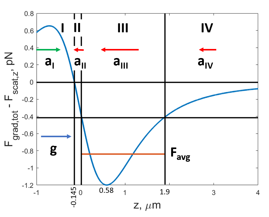
Figure 3: Gradient and scattering forces equilibrium on the $z$ axis. The particle is falling from the left, in the direction of the gravitational acceleration, g, indicated by the blue arrow. Its diameter is $100$nm and the laser parameters are: $100$mW, $1550$nm. The focusing element is an NA$=$1 parabola of $3.6$mm diameter. In the first region, I, where $F_{grad}>F_{scat}$, the particle receives an additional acceleration, $a_{I}$, from the gradient force. The second region, II, begins at $145$nm in front of the focal plane, where $F_{grad}=F_{scat}$ for the particle considered, and ends at $z=0$, where $F_{grad}=0$. Here, the deceleration begins, because the scattering force is greater than, and of opposite sign to, the gradient force. In the third region, III, both forces act in the direction opposite to that of the particle. The deceleration, $a_{III}$, is highest here, with a peak at $0.58\mu$m. The red, horizontal line, marks the average force of this region, denoted $F_{avg}$. Its value is $-0.84$pN. In the fourth region, after 1.9$\mu$m, the deceleration drops because both forces fade away as we depart from the focal plane.

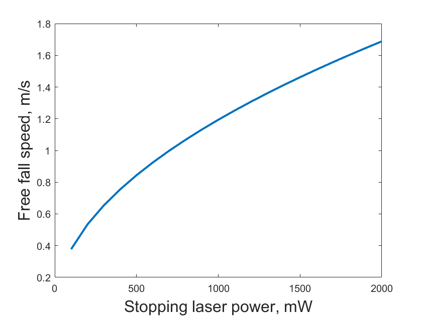
Figure 4: Particle return speed against trap power needed to stop it. To stop a particle returning at $1.4$ m/s, we need a laser power of $1.5$ W.

The problem now is whether we can stop the particle in the available $2\mu$m interval. The stopping strength of the average force, $F_{avg}$ may be written as:

$$F_{avg}\cdot d=\frac{mv^{2}}{2},$$ (13)

where $d$ is the distance over which the average force acts, $m$ is the particle mass and $v$ is the highest velocity that the force can stop over this distance. From here we extract the maximal velocity to be:

$$v_{max}=\sqrt{\frac{2\cdot 8.4\cdot 10^{-13}\cdot 1.9\cdot 10^{-6}}{2.2\cdot 10^{-17}}}=0.38\rm{ms}^{-1}.$$ (14)

This is less than half of the expected return velocity. Figure 4 shows the required laser power to stop a particle depending on its return velocity. We see that in order to stop, for example, a $1.4$ms^-1 particle, we would need a laser power of $1.5$W, whilst our trap typically operates at $100$mW. We must note that only the scattering force is dissipative and actually takes away energy from the falling particle. The gradient force will spring the particle back upwards after the latter was brought to a halt. So, in order to properly brake the particle, one would need to modulate the laser power, in synchronization with the motion of the particle, starting from $1.5$W down to the $100$mW stationary trapping power, until the latter is brought to the stationary regime, where the regular feedback cooling protocol can be applied.

V Results

V.1 Expected Interference Patterns

We now present our expected interference patterns for particles of mass $10^{6}$ and $10^{8}$ atomic mass units, as well as how the fringe visibility varies as we change various parameters. Figure 5 shows both the expected quantum interference patterns, with decoherence sources included, and the classically predicted Moiré shadow patterns for the two masses of particles we have investigated.

Table 1: Table of relevant parameters used for the generation of quantum and classical patterns throughout this section.

Parameter	$10^{6}$ amu particle	$10^{8}$ amu particle
Initial temperature	1mK	1mK
Pressure	$10^{-10}$ mbar	$10^{-10}$ mbar
Flight time	29ms	71ms
Phase modulation($\phi_{0}$)	$\pi/2$	$8\pi$

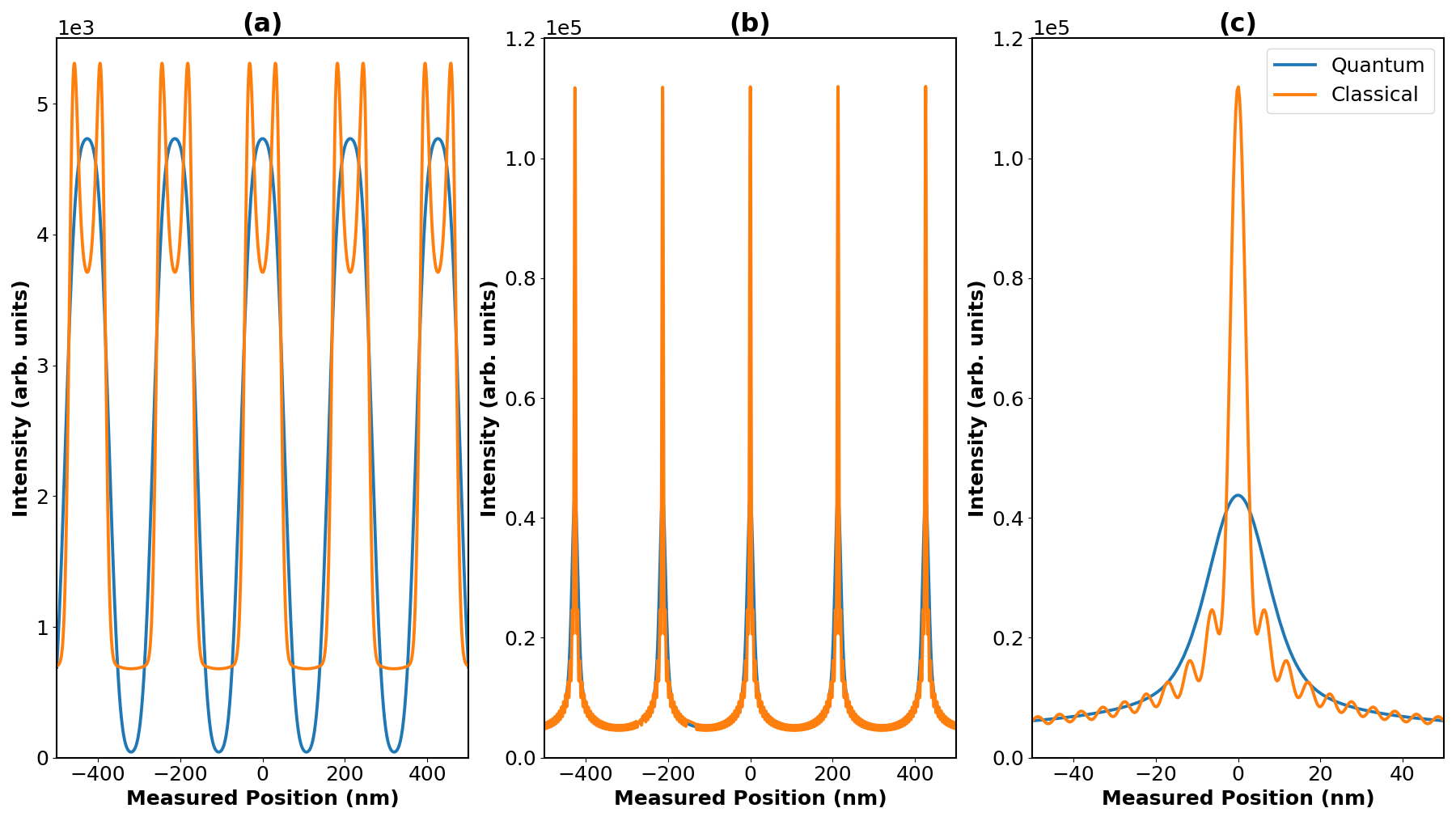
Figure 5: Simulated quantum interference patterns (blue) and Moiré shadow patterns (orange) for a (a) $10^{6}$ amu nanoparticle and (b) a $10^{8}$ amu nanoparticle. (c) shows a zoomed in section of (b) for clarity. These patterns assume parameters which were found by optimising for the visibility of the quantum fringes in each case and are detailed in table 1. These patterns include all interference effects mentioned in the previous section aside from the decoherence from imperfect kicks which is shown later.

An important point to make about the parameter selection shown in Table 1 is the short flight time selected for the high mass particle. We mentioned previously that, to be confident in seeing quantum interference effects, the state should be allowed to evolve for a time on the order of the Talbot time before interacting with the grating. The Talbot time for the $10^{8}$amu particle is around $2.8$s and yet we have selected a time of 71ms, several orders of magnitude lower. The reasoning for this is that in order to achieve a flight time on the order of the Talbot time, the interferometer would have to be much taller, on the order of meters or tens of meters. We would still need to recapture the particle in our optical trap, which has a recapturing range on the order of microns. For recapture to be achieved for these flight times we would require levels of cooling several of orders of magnitude beyond what has been achieved experimentally to date. Even a 10cm height would translate to cooling requirements below the ground state on the order of nano-Kelvin. For this reason we restricted our investigation to tens or hundreds of milliseconds, resulting in significantly sub-Talbot times for the higher mass case. Nonetheless our simulations show clear high visibility fringes even when working in this regime as demonstrated in Figure 5.

V.2 Quantum/Classical Distinctions

As we see in Figure 5 (b) and (c), it can be quite difficult to distinguish between the quantum and classical predictions especially when working with the higher mass particles in the sub-Talbot regime. To distinguish between the two predictions in the high mass case would require spatial resolution in our measurements on the order of nanometers. While not impossible this would certainly be another highly demanding requirement. For this reason we propose alternative means by which to differentiate between the quantum and classical case. By generating many interference patterns whilst varying either the phase modulation parameter ($\phi_{0}$) or the flight time, for example, and recording the visibility of the observed fringes, we can construct plots with clearer distinctions for the quantum and classical case. Figures 6 and  7 demonstrate this idea. Aside from the one which are changing, the parameters used for these plots are the same as those detailed in table  1.

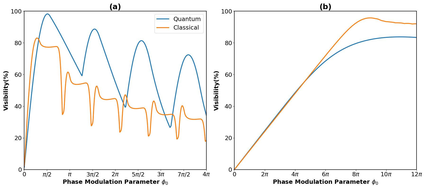
Figure 6: Expected variation of quantum (blue) and classically (orange) predicted visibilities of fringes when varying the phase modulation parameter $\phi_{0}$, controlled by the pulse energy of the grating laser. (a) shows the expected visibility variation for a SiO2 particle of mass $10^{6}$amu whilst (b) demonstrates the same plot for a particle of mass $10^{8}$amu.

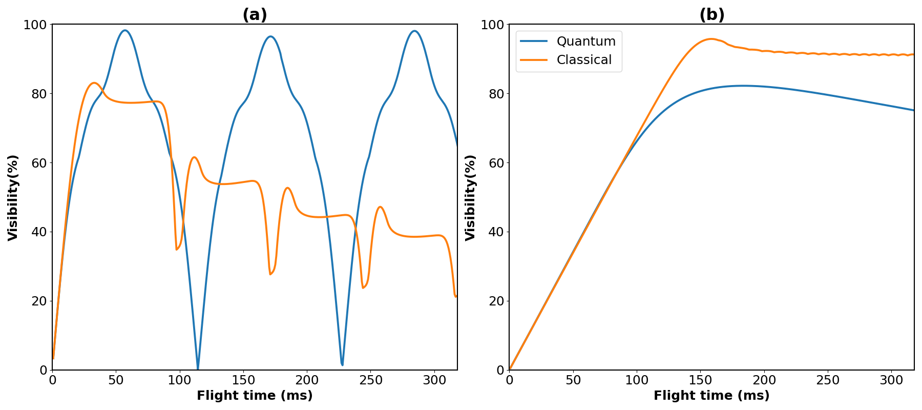
Figure 7: Expected variation of quantum (blue) and classically (orange) predicted visibilities of fringes with varying flight times. (a) shows visibility variation for a $10^{6}$amu SiO2 particle, whilst (b) shows the same plot for a $10^{8}$amu particle.

The differences in the quantum and classical predictions is once again most clear for the $10^{6}$amu particle which has the privilege of working in the Talbot regime. Nonetheless we now see distinctive differences in the predicted visibilities of the quantum and classical models even for the $10^{8}$amu particle. The models diverge from each other when dealing with longer time of flight and larger values of the phase modulation parameter. By conducting such experiments the quantum and classical descriptions could be more easily distinguished when the required spatial resolution to distinguish them from a single interference pattern is too challenging to achieve. A final point to make is that the parameters used within these simulations where chosen by optimising for the highest visibility of quantum fringes in each case. It would be entirely possible to instead optimise for the largest divergence between quantum and classical visibility predictions instead, whilst sacrificing overall visibility. Since our predicted visibilities are relatively high, even when accounting for major sources of decoherence, this could be a valuable method to ensure our ability to distinguish between quantum and classical predictions.

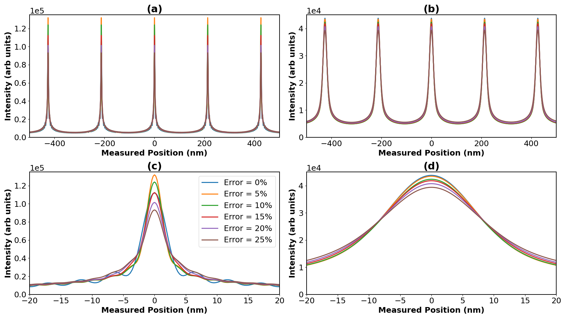
Figure 8: Expected interference patterns for the interferometry of a $10^{8}$ amu SiO2 particle when accounting for error in initial kick velocity, with errors ranging from 0 to 25%. (a) shows the expected patterns for the classical case whilst (b) shows the quantum case. (c) and (d) give a zoomed in picture of (a) and (b) respectively.

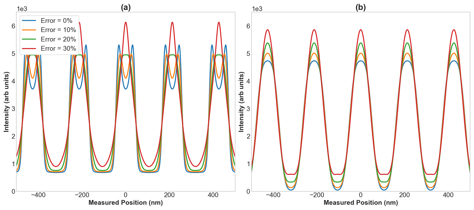
Figure 9: Expected interference patterns for the interferometry of a $10^{6}$ amu SiO2 particle when accounting for error in initial kick velocity, with errors ranging from 0 to 30%. (a) shows the expected patterns for the classical case whilst (b) shows the quantum case.

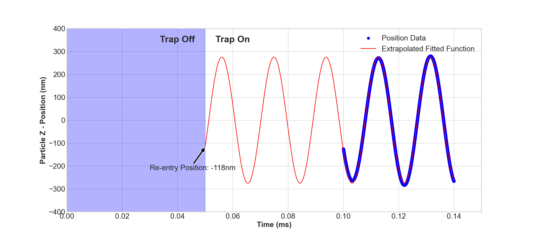
Figure 10: Example of a measurement of a particle’s re-entry position in the vertical ($Z$) direction. The trap was turned off at $0$ ms and turned back on at $0.05$ ms. Position is measured from the equilibrium position of the particle, which is slightly offset from the center of the trap.

V.3 Throw and Catch Specific Decoherence

As previously mentioned the plots shown up to this point do not consider the decoherence associated with imperfect control of the energy of the kicking pulse and therefore imperfect flight times. We now demonstrate the effects of this source of decoherence on the visibility of our fringes. Figures 8 and  9 show how varying errors of initial velocity impact visibility for the case of a $10^{8}$ amu particle and a $10^{6}$ amu particle respectively. Once again the parameters for these plots are the same as those detailed in table 1. These plots were generated by simulating many interference patterns, with flight times varying according to a normally distributed velocity profile for the initial kick, and then averaged into the overall expected pattern. In these plots the error refers to the standard deviation of this velocity distribution.

The results shown in Figure 8 are not particularly surprising since we are working in the sub-Talbot regime. As we saw in Figure 7(b) this means that variation in visibility with flight time is relatively slow and smooth. Hence, we would expect a slow decrease in visibility with increase in initial velocity error whilst not expecting a significant change in the shape of the pattern. This is exactly what Figure 8 shows although we do also see the washing out of the detail beyond the central fringe for the classical case. Figure 9 on the other hand is a bit different. Whilst the quantum case once again shows a slow decrease in visibility, the classical case now also shows a change in the shape of the pattern. In fact we see that the overall positioning of the fringes for the two regimes converge with increasing error. This could mean that the quantum and classical patterns could look quite similar to each other if the error in the initial kick velocity is high even for a $10^{6}$amu particle. Nonetheless the key takeaway from these plots is that even very large errors of 25% or 30% still lead to high visibility fringes which implies this is a very manageable source of extra decoherence. The explicit visibility values for the plots are provided below in tables  2 and  3.

Table 2: Table of visibility values for the plots presented in figure 8 for a $10^{8}$ amu particle.

Error	Classical Visibility	Quantum Visibility
0%	92.2%	79.6%
5%	93.0%	79.6%
10%	92.5%	79.1%
15%	91.5%	78.4%
20%	90.3%	77.2%
25%	89.0%	75.5%

Table 3: Table of visibility values for the plots presented in figure 9 for a $10^{6}$ amu particle.

Error	Classical Visibility	Quantum Visibility
0%	77.3%	98.2%
10%	75.0%	94.9%
20%	73.5%	88.3%
30%	74.5%	81.1%

V.4 Experimental Progress

Since much has already been published on the trapping and cooling aspects that will be used in this experiment, here we give a preliminary demonstration of how the measurement portion of the interferometer will be achieved. Inspired by Hebestreit et al. [13] we tested our measurement scheme by performing release and re-capture experiments. Once the particle was prepared in the state we desire before starting interferometry, we turned off the trap for $50\mu$s and then turned it back on. We then observed the oscillations immediately after the trap was turned on. By filtering for a desired direction of oscillation and then fitting to the filtered data, we are able to extract the re-entry position. This procedure is illustrated in figure 10.

We can estimate a rough precision of this technique by taking different length segments of the data, applying the same process, and seeing how much the re-entry position varied as a result. When this was done we found that all extracted positions lay within $15$ nm of each other. This should already be sufficient for our purposes. This was just a demonstration of the idea behind our detection scheme and not the final product. Work is ongoing for using more sophisticated techniques for extracting the position at which the particle re-enters the trap, such as using a particle filter [19].

VI Conclusion

By building upon previous ideas for how wave-like behaviour could be observed for high mass particle, we have presented a throw and catch scheme which we believe will be able to generate quantum interference patterns of nanoparticles, with masses up to three order of magnitude greater than the current matter-wave interferometry record. Whilst maintaining the easy to achieve conditions of previous proposals, such as a room temperature environment and using only a single optical diffraction element, we have shown how the problems associated with inefficient loading can be sidestepped without the introduction of significant extra decoherence. We have shown how the Talbot effect can be used to generate similar interference patterns to what has been discussed previously with our new proposed set-up. Accounting for all major sources of decoherence and working with similar masses to what has been discussed before, that being $10^{6}$ amu particles, we found the possibility for high visibility fringes with a clear distinction between the quantum and classical predictions, all while adhering to the practical limitations associated with recapturing the particle. We have shown that this system could even be used for particle masses in the region of $10^{8}$ amu by working with flight times below the Talbot time, although in this case with more similarity between the quantum and classical predictions.

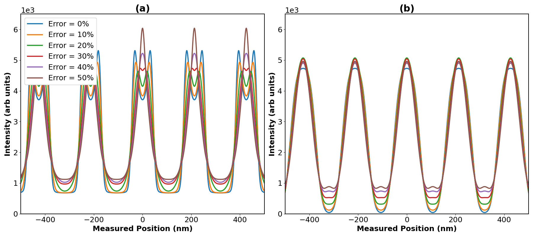
Figure A0: Expected interference patterns for the interferometry of a SiO2 particle, with mean mass of $10^{6}$amu, when accounting for a spread of different particle masses being used for each run of the experiment. Errors in mass range from 0 to 50%. (a) shows the expected patterns for the classical case whilst (b) shows the quantum case.

Appendix A Incoherent sources

Table 4: Table of visibility values for the plots presented in figure A0.

Mass Error	Classical Visibility	Quantum Visibility
0%	77.3%	98.2%
10%	75.6%	95.1%
20%	72.4%	88.3%
30%	66.0%	81.1%
40%	67.1%	74.5%
50%	68.7%	71.4%

To demonstrate the advantage of re-using the same SiO₂ particle for every run of our interferometer, we performed simulations which allowed the mass of the particle used for each run to vary. This would roughly simulate the situation where a new particle would be reloaded for each run. Figure A0 shows the results of these simulations when particles of mean mass $10^{6}$amu were used; with other parameters matching those listed in table 1. Table 4 shows that the visibility of the fringes, that we expect to see in the quantum interference pattern, decreases as the spread of masses that the particles can take increases. In figure A0 we also see that if the spread in mass of the particles exceeds $30\%$ then the maximal intensity regions of the quantum and classically predicted interference patterns will overlap, leading to additional difficulty in distinguishing between the two cases. Therefore, we see that re-using the same particle can lead to drastic increases in visibility depending on the variation in mass of the different particles that would be used otherwise. It is also important to note that these simulations only took into account a change in mass of the particle. In reality, different particles could have different shapes or densities depending on the purity of the batch that is being used. This would lead to even further washing out of the fringes. We also note that these visibility drops could be partially avoided, when not re-using the same particle, by post-selecting data where only similar particles where used. However, this would lead to more runs being necessary, where again the problem of inefficient re-loading arises.

Appendix B Mie Scattering Correction

As stated in the main text, in our simulations we implemented a correction with respect to the results in [14] for what concern the decoherence reduction factor induced by the scattering of grating photons in the Mie scattering regime, i.e., accounting for the finite size of the particles.

We closely follow the treatment in [14]. Under the assumption that the laser waist is much larger than the size of the particle, the effect of scattering of grating’s photons is described by the action of the Lindblad super-operator

$$\mathcal{L}[\rho_{S}] =|\alpha|^{2}\sum_{\nu}\int d\bm{k}\delta(\omega_{k}-\omega_{0})\left(2\mathcal{T}_{\bm{k}\nu,c}(\hat{r})\rho_{S}\mathcal{T}^{*}_{c,\bm{k}\nu}(\hat{r})-\left\{|\mathcal{T}_{\bm{k}\nu,c}(\hat{r})|^{2},\rho_{S}\right\}\right)$$

where the collisional operators are

$$\mathcal{T}_{\bm{k}\nu,\bm{c}}(\hat{\bm{r}})=\sum_{\nu^{\prime}}\int d\bm{k}^{\prime}\langle{\bm{c}}|{\bm{k}^{\prime},\nu^{\prime}}\rangle\mathcal{T}^{*}_{\bm{k}^{\prime}\nu^{\prime},\bm{k}\nu}(\hat{\bm{r}}).$$ (16)

For our case of interest, $\ket{\bm{c}}$ is a linearly polarized standing wave with mode volume $V_{0}$ such that

$$\bra{\bm{k},\nu}{\bm{c}}\rangle =\frac{1}{V_{0}}\int d\bm{x}\,e^{-i\bm{k}\cdot\bm{x}}\bm{\epsilon}_{\bm{k},\nu}\cdot\bm{\epsilon_{d}}\,g(x,y)\cos(k_{0}z)$$

$$\simeq\frac{\bm{\epsilon}_{\bm{k},\nu}\cdot\bm{\epsilon}_{k_{z},\nu^{\prime}}}{\sqrt{V_{0}}}\tilde{g}(k_{x},k_{y})\delta(k_{z}^{2}-\omega_{0}^{2})\simeq\frac{\omega_{0}\bm{\epsilon}_{k,\nu}\cdot\bm{\epsilon}_{k_{z},\nu^{\prime}}}{\sqrt{V_{0}}}\tilde{g}(k_{x},k_{y})\delta(k_{x})\delta(k_{y})\delta(k_{z}-\omega_{0}^{2}).$$ (17)

where g(x,y) represents the laser transverse beam profile and $\tilde{g}(k_{x},k_{y})$ its Fourier transform. Notice that the approximation made in the last line is justified under the assumption of a laser field with a very wide spot area $a_{g}$, i.e. $a_{g}\gg k_{0}^{2}$

We thus have for the collisional operators

$$\mathcal{T}_{\bm{k}\nu,\bm{c}}(\hat{\bm{r}})\simeq\frac{1}{4\pi\omega_{k}\sqrt{V_{0}}}\left(e^{-i\bm{k}_{0}\cdot\hat{\bm{r}}}f^{*}_{\nu_{0},\nu}(\bm{k_{0}},\bm{k})+e^{i\bm{k}_{0}\cdot\hat{\bm{r}}}f^{*}_{\nu_{0},\nu}(-\bm{k_{0}},\bm{k})\right),$$ (18)

with $f_{\nu,\nu^{\prime}}(\bm{k},\bm{k}^{\prime})$ the Mie scattering amplitude.

Considering the incoming standing wave polarized along the $x$ direction we obtain the vectorial scattering amplitude

$$\sum_{\nu}\epsilon_{\nu}f^{*}_{\nu,{x}}(\bm{k_{0}},\bm{k})=(S_{2}\cos\phi\epsilon_{\theta}-S_{1}\sin\phi\,\epsilon_{\phi}).$$ (19)

Here, $\epsilon_{\theta}\cdot\epsilon_{\phi}=0$ as they are two orthogonal components of the scattered field polarization. For the explicit expressions for $S_{1}$ and $S_{2}$ we refer the reader to Appendix A of [14].

We then finally arrive to rewrite the Liouvillian super-operator in the form

$$\mathcal{L}[\rho_{S}] =|\alpha|^{2}\sum_{\nu}\int d\bm{k}\delta(\omega_{k}-\omega_{0})\left(2\mathcal{T}_{\bm{k}\nu,c}(\hat{r})\rho_{S}\mathcal{T}^{*}_{c,\bm{k}\nu}(\hat{r})-\left\{|\mathcal{T}_{\bm{k}\nu,c}(\hat{r})|^{2},\rho_{S}\right\}\right)$$

$$=|\alpha^{2}|\int d\bm{k}\delta(\omega_{k}-\omega_{0})\left(2\mathcal{T}_{\bm{k}\phi,c}(\hat{r})\rho_{S}\mathcal{T}^{*}_{c,\bm{k}\phi}(\hat{r})-\left\{|\mathcal{T}_{\bm{k}\phi,c}(\hat{r})|^{2},\rho_{S}\right\}\right)$$

$$+|\alpha^{2}|\int d\bm{k}\delta(\omega_{k}-\omega_{0})\left(2\mathcal{T}_{\bm{k}\theta,c}(\hat{r})\rho_{S}\mathcal{T}^{*}_{c,\bm{k}\phi}(\hat{r})-\left\{|\mathcal{T}_{\bm{k}\theta,c}(\hat{r})|^{2},\rho_{S}\right\}\right)$$ (20)

From this last expression, following [14] we finally arrive at the correct form of their Eq. (28) which reads

$$R_{\rm sca}(z_{-},z_{+})=\exp\left[F(s)+a(s)\cos(2kz)+ib(s)\sin(2kz)\right],$$ (21)

with now the coefficients given by

$$a(s) =\frac{2\pi c}{V_{0}}\int d\tau|\alpha(\tau)|^{2}\int d\Omega\,{\rm Re}\big{(}\mathbb{f}^{*}(k,k\mathbb{n})\cdot\mathbb{f}(-k,k\mathbb{n})\big{)}[\cos(kn_{z}s)-\cos(ks)],$$

$$b(s) =\frac{2\pi c}{V_{0}}\int d\tau|\alpha(\tau)|^{2}\int d\Omega\,{\rm Im}\big{(}\mathbb{f}^{*}(k,k\mathbb{n})\cdot\mathbb{f}(-k,k\mathbb{n})\big{)}\sin(kn_{z}s),$$

$$F(s) =\frac{2\pi c}{V_{0}}\int d\tau|\alpha(\tau)|^{2}\int d\Omega\,|\mathbb{f}(k,k\mathbb{n})|^{2}[\cos((1-n_{z})ks)-1].$$ (22)

with $\mathbf{f}(k,k\mathbb{n})=(f^{\parallel}(k,k\mathbb{n}),f^{\perp}(k,k\mathbb{n}))^{T}$ and

$$f^{\parallel}(k,k\mathbb{n})=S_{1}\cos\phi$$ (23)

$$f^{\perp}(k,k\mathbb{n})=S_{2}\cos\phi$$ (24)