Implementation of the Emulator-based Component Analysis

Abstract

We present a PyTorch-powered implementation of the emulator-based component analysis used for ill-posed numerical non-linear inverse problems, where an approximate emulator for the forward problem is known. This emulator may be a numerical model, an interpolating function, or a fitting function such as a neural network. With the help of the emulator and a data set, the method seeks dimensionality reduction by projection in the variable space so that maximal variance of the target (response) values of the data is covered. The obtained basis set for projection in the variable space defines a subspace of the greatest response for the outcome of the forward problem. The method allows for the reconstruction of the coordinates in this subspace for an approximate solution to the inverse problem. We present an example of using the code provided as a Python class.

I Introduction

Inverse problems consist of reconstructing input data $\mathbf{X}$ or parameters of a model from a later observation of a dependent response $\mathbf{Y}$. In addition to their rich heritage from pure mathematics Kaipio2005 ; Calvetti2018 ; Uhlmann2014 , many applied inverse problems originate from geophysics Tarantola1982 . Other modern examples of the applied problems include tomography Arridge2009 (as a part of the more general image/signal processing problem) and spectroscopy. Inverse problems can be identified in a wealth of research contexts, and their approximate solutions are traditionally searched for by regularization or by Bayesian procedures Kaipio2005 ; Mohammad-Djafari2022 .

For example, given an atomistic structure with a charge state, the resulting electronic spectrum (ultraviolet/visible, X-ray, etc.) is defined by the quantum-mechanical electronic Hamiltonian of the system. The formed map is certainly nonlinear in terms of structure, and not necessarily an injective function. Moreover, some structural degrees of freedom may account for huge spectral responses while some may result little or virtually none. As often the case with inverse problems, full reconstruction of structural parameters is an ill-posed problem, and already identification of the relevant structural degrees of freedom may be a worthwhile scientific result. It may likewise be important to filter out structural degrees of freedom without spectral response to achieve a more well-posed inverse problem of reconstruction of structural information from the respective spectra Vladyka2023 .

Machine learning (ML) opens new possibilities for solving inverse problems. With the backpropagation algorithm Rumelhart1986 and graphics processing units (GPU), training of extensive neural networks (NN) has become feasible. Because the NN is a universal approximator Hornik1989 ; Cybenko1989 ; Leshno1993 , mimicking many forward problems is possible given that enough data is available for the task. The complete solution of a potentially ill-defined inverse problem may still be difficult, but an approximative one may be obtained by first identifying the reconstructable information. To do this, the fast evaluation of the forward problem by NN may be utilized in iterative procedures. We propose the emulator-based component analysis (ECA) Niskanen2022 as a tool in finding a fast approximate solution for nonlinear inverse problems.

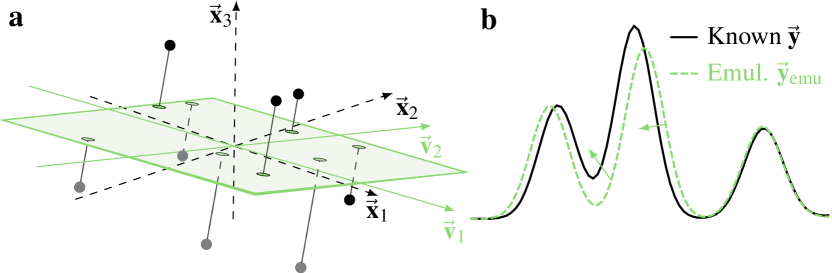
Figure 1: The principle of ECA illustrated for 2 ECA components $\{\mathbf{v}_{1},\mathbf{v}_{2}\}$ in a 3-dimensional $\mathbf{X}$ space $\mathrm{span}\{\mathbf{x}_{1},\mathbf{x}_{2},\mathbf{x}_{3}\}$ (a). The ECA components (basis vectors) are selected by iterative optimization so that emulated $\mathbf{y}_{\mathrm{emu}}$ for the projected data points match closest with the known $\mathbf{y}$ of the original data (b).

The ECA algorithm aims for dimensionality reduction by projection on basis vectors in the input space $\mathbf{X}$ while maximizing the variance of a dependent target variable of the forward problem in space $\mathbf{Y}$ of vectors $\mathbf{y}=\mathbf{y}(\mathbf{x})$. Thus ECA belongs to the family of ‘projection pursuit’ algorithms Kruskal1969 ; Friedman1974 ; Huber1985 and is closely related to projection pursuit regression (PPR) Friedman1981 . However, instead of using an unknown smoothing function (ridge function), ECA utilizes a more general and pre-selected function: a machine learning model (i.e. a NN) acting as an emulator for the forward problem $\mathbf{y}_{\mathrm{emu}}(\mathbf{x})\approx\mathbf{y}(\mathbf{x})$. For example, in spectroscopy studies, such emulator would predict a spectrum for the corresponding atomistic structure. Approximate solution $\mathbf{x}^{\prime}$ of the inverse problem $\mathbf{y}\rightarrow\mathbf{x}$ may then be found for the obtained dimensionally-reduced space. In this contribution we present an efficient numerical implementation of the ECA algorithm and its application for the inverse problem together with an example.

II Definition

The result of ECA is an orthogonal set of vectors $\mathbf{V}=\{\mathbf{v}_{j}\}_{j=1}^{k}$ in X space. These vectors are optimized using data $\{(\mathbf{x}_{i},\mathbf{y}_{i})\}$ separate to those used for emulator training, so that most variance of vectors $\mathbf{y}_{i}$ is covered by emulator prediction $\mathbf{y}_{\mathrm{emu}}(\tilde{\mathbf{x}}_{i}^{(k)})$ subsequent to projection of vectors $\mathbf{x}_{i}$ onto $\mathbf{V}$

$$\tilde{\mathbf{x}}_{i}^{(k)}=\sum_{j=1}^{k}\underbrace{(\mathbf{v}_{j}\cdot\tilde{\mathbf{x}}_{i})}_{=:t_{i,j}}\mathbf{v}_{j}.$$ (1)

The algorithm is designed to work with z-standardized $\mathbf{X}$ data points $\tilde{\mathbf{x}}_{i}$ (corresponding to $\mathbf{x}_{i}$) for which Equation (1) represents a reduction to $k$ dimensions. The coordinates of the data point $\tilde{\mathbf{x}}^{(k)}_{i}$ reduced dimension ($\mathbf{t}$ scores) read $\mathbf{t}_{i}=(t_{i,1},...,t_{i,k})$. The idea is depicted in Figure 1.

As a metric for the optimization of $\mathbf{V}$, we use a generalized covered variance (R²-score). Organizing z-standardized Y data points $\tilde{\mathbf{y}}_{i}$ as row vectors of matrix $\mathbf{Y}$, and the corresponding predicted data points $\mathbf{y}_{\mathrm{emu}}(\tilde{\mathbf{x}}_{i}^{(k)})$ as row vectors of matrix $\mathbf{Y}^{\mathrm{(pred)}}$, this is defined as:

$$\rho=1-\frac{\mathrm{tr}\left(\bar{\mathbf{Y}}^{T}\bar{\mathbf{Y}}\right)}{\mathrm{tr}\left(\mathbf{Y}^{T}\mathbf{Y}\right)}$$ (2)

where $\bar{\mathbf{Y}}=\mathbf{Y}-\mathbf{Y}^{\mathrm{(pred)}}$.

The procedure utilizes iterative optimization of the basis vectors so that $\rho$ is maximized for the used data. The method proceeds one vector $\mathbf{v}_{j}$ at a time where orthonormality is enforced after optimization of each vector. We note that the replacing any of the ECA basis vector $\mathbf{v}_{i}$ with its opposite $-\mathbf{v}_{i}$ does not affect the covered variance, but only changes the sign of the corresponding $\mathbf{t}_{i}$ score.

The expansion $\tilde{\mathbf{x}}_{i}^{(k)}$ gives an approximation of point $\tilde{\mathbf{x}}_{i}$ (and $\mathbf{x}_{i}$ after inverse z-standardization), in the subspace $\mathrm{span}(\mathbf{V})$, which $\mathbf{Y}$ by design shows greatest response to. We approach the inverse problem by deducing the respective coordinates $\mathbf{t}^{\prime}$ for a given $\mathbf{y}$, and $\tilde{\mathbf{y}}$, after which the approximate solution is

$$\tilde{\mathbf{x}}^{\prime}=\sum_{j=1}^{k}t_{j}^{\prime}\mathbf{v}_{j}.$$ (3)

This reconstruction utilizes numerical optimization for $\mathbf{t}^{\prime}$ for given $\mathbf{y}$ and $\mathbf{V}$. The approximate solution $\mathbf{x}^{\prime}$ in $\mathbf{X}$ space is obtained via z-score inverse transformation.

III Implementation

The module is written in Python utilizing PyTorch pytorch (>2.0). The use of PyTorch offers some benefits:

1. Runs very efficiently owing to automatic differentiation approach implemented in this package.

2. Can easily be run in parallel over multiple CPU cores or GPU.

3. It provides more control during the fitting procedure than some other optimization toolkits, (e.g., scipy.optimize Scipy ).

We arranged the search for ECA vectors as a mini-batch optimization using the Adam optimizer Adam . The algorithm utilizes previously found component vectors, and orthogonality of the search is forced by allowing optimization steps only in their orthogonal complement. The workflow of the procedure is presented in Algorithm 1 and the optimization options together with their default values are given in Table 1. The full reference manual and a sample code for the implementation are available in the Appendix.

Trained emulator $\mathbf{y}_{\mathrm{emu}}:\mathbf{x}\to\mathbf{y}$

Data $(\mathbf{X,Y})$

Initialize first vector: $\mathbf{v}_{1}\leftarrow\mathrm{rnd()}$

while $\mathbf{v}_{1}$ not optimized do

     Calculate projection: $\mathbf{X}_{\mathrm{proj}}\leftarrow(\mathbf{X}\cdot\mathbf{v}_{1})\cdot\mathbf{v}_{1}$

     Optimize $\mathbf{v}_{1}$ : $\rho(\mathbf{Y},\mathbf{y}_{\mathrm{emu}}(\mathbf{X}_{\mathrm{proj}}))\to max$

     Normalize $\mathbf{v}_{1}\leftarrow\mathbf{v}_{1}/|\mathbf{v}_{1}|$

end while

Initialize the basis set: $\mathbf{V}_{1}\leftarrow\mathbf{v}_{1}$

for rank $i\leftarrow 2,\ldots,k$ do

     Initialize $i$-th component: $\mathbf{v}_{i}\leftarrow\mathrm{rnd()}$

     while $\mathbf{v}_{i}$ not optimized do

         Calculate projection: $\mathbf{X}_{\mathrm{proj}}\leftarrow(\mathbf{X}\cdot\mathbf{V})\cdot\mathbf{V}+(\mathbf{X}\cdot\mathbf{v}_{i})\cdot\mathbf{v}_{i}$

         Optimize $\mathbf{v}_{i}$ : $\left(\rho(\mathbf{Y},\mathbf{y}_{\mathrm{emu}}(\mathbf{X}_{\mathrm{proj}}))\to max\right)$ $\cap\left(\mathbf{V}\cdot\mathbf{v}_{i}=0\right)$ $\triangleright$ $\mathbf{v}_{i}$ is orthogonal to vector space $\mathbf{V}$

         Normalize $\mathbf{v}_{i}\leftarrow\mathbf{v}_{i}/|\mathbf{v}_{i}|$

     end while

     Append optimized component to the basis: $\mathbf{V}_{i}\leftarrow\mathbf{v}_{i}$

end for

Algorithm 1 ECA implementation

Reproducibility of the results is satisfied by setting the seed for the random numbers generator via seed parameter of the options or by calling set_seed() method. The fit() method also allows the manual step by step evaluation and re-evaluation of the components by specifying keep=n argument: a positive value is interpreted as ‘start after $n$-th component’, and for negative values the last $|n|$ calculated components are removed, evaluation starts after the remaining ones.

In addition to providing the ECA basis vectors for the data–emulator pair, the presented implementation carries out typically used transformations. These functionalities are presented in Figure 2.

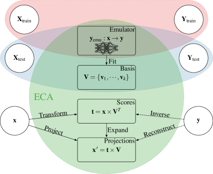
Figure 2: Schematics of ECA functionality. ECA uses an emulator, trained on $(\mathbf{X},\mathbf{Y})_{\mathrm{train}}$, validated on $(\mathbf{X},\mathbf{Y})_{\mathrm{test}}$. Fitting of the ECA object on $(\mathbf{X},\mathbf{Y})_{\mathrm{test}}$ (or $(\mathbf{X},\mathbf{Y})_{\mathrm{train}}$) results in a basis set $\mathbf{V}$. ‘Transform’ and ‘project’ operations are linear transformations of the input vector $\mathbf{x}$. On the contrary, ‘inverse’ and ‘reconstruct’ are implemented using optimization algorithms. These are not linear operations and may produce ambiguous results for the complex (highly multidimensional) systems.

Table 1: The list of options for both forward and inverse algorithms.

Parameter	Explanation	Default	(inv)
lr	Learning rate for the Adam optimizer	$10^{-3}$	$0.05$
betas	Beta parameters for the Adam optimizer (see Adam )	(0.9, 0.999)	(0.9, 0.999)
tol	Stopping condition	$10^{-4}$	$10^{-4}$
epochs	Max. number of epochs	$10^{4}$	$10^{3}$
batch_size	Mini-batch size (forward only)	200	—
seed	Seed for random number generator	None	None

In this work, we propose to utilize dimensionality reduction achieved via projection of the $\mathbf{X}$ data onto ECA space for approximation of the inverse problem solution. The inverse() method is searching for the points in ECA space ($\mathbf{t}$ scores) for which the emulator provides the best match with given $\mathbf{y}$, while the reconstruct() method is performing inverse transformation followed by its expansion to $\mathbf{X}$ space. In other words, it returns an $\mathbf{x}^{\prime}$, which predicts to the best match with given $\mathbf{y}$. The obtained $\mathbf{t}^{\prime}$ scores can be used for studying the differences in the data, e.g., via possible grouping, cluster analysis etc, and interpretability of $\mathbf{x}^{\prime}$ vectors allows to find the relation between $\mathbf{x}$ and $\mathbf{y}$ in a significantly more lightweight way than an exact solution of the inverse problem would.

The PyTorch implementation, while robust and efficient, requires an emulator implemented in PyTorch. Numerous machine learning libraries exist and provide a similar functionality. A simple feed-forward network can be transferred between the implementations by specifying the matrices, bias vectors and activation functions. We provide a script which allows to convert a trained sklearn-based multilayer perceptron (sklearn.MLPRegressor scikit-learn ) into an equivalent PyTorch-based neural network for use with the PyTorch-based ECA.

IV Example

As an example, we present the analysis of simulated N K-edge near-edge X-ray absorption fine structure (NEXAFS) of aqueous triglycine Eronen2023 . This data consists of local structural descriptors (local version of the many-body tensor representation, LMBTR Huo2022 , implemented in Himanen2020 ) and related core-level spectra, available at triglydata . The descriptors are built from atomistic structures, consisting of the single triglycine molecule and the water molecules within 3 Å from it. The spectral data are given as intensities of the three regions of interest (ROIs; I–III). The purpose of the analysis is to discover spectrally dominant structural modifications, i.e. finding structural degrees the change of which results in the most change in the spectra. ECA was applied as in the original paper: the components were obtained with an ECA fit data set of 3000 data points and the results were validated with ECA validation data set of 2999 data points. The original emulator was trained on 23996 data points, and for this work it was simply converted (by replicating its architecture and weights) to PyTorch. The scripts of our implementation for this data are provided with the codes.

ECA covered variance up to rank five is given in Table 2 and closely resembles the original work. The LMBTR descriptor allows for an interpretation of the deduced basis vectors in terms of the structural features. Figure 3 presents the first basis vector which describes the interatomic distance distributions (from each active nitrogen site N_ex). These results are also in agreement with the previous ones. Moreover, whereas the principal component analysis (PCA) of the structural descriptor shows two distinct regions, we showed that this information is lost in ROIs of NEXAFS, and therefore can not be recovered by X-ray absorption experiments. The results, available in the scripts provided with this work, were the same with the presented implementation.

Table 2: The covered spectral ROI variances as a function of the rank of the ECA.

Rank	ECA	ECA
	fit	validation
1	0.535	0.516
2	0.747	0.710
3	0.850	0.810
4	0.865	0.811
5	0.874	0.817

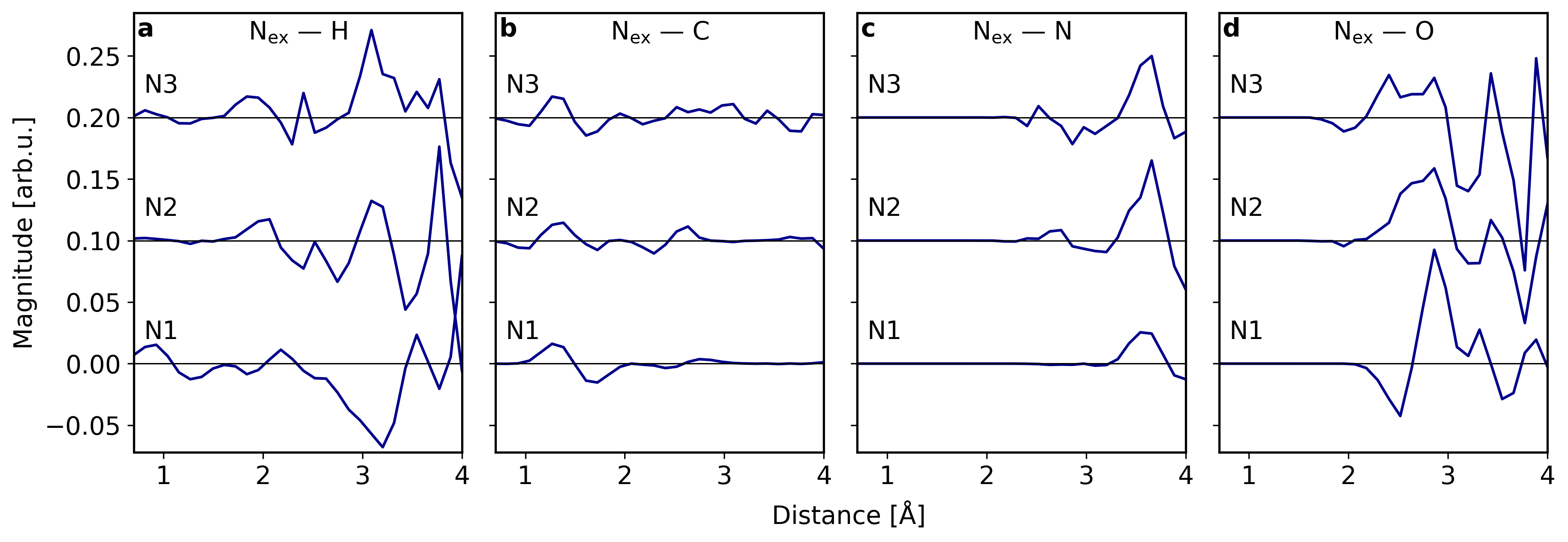
Figure 3: The interatomic distance distribution part of the first component vector for the example of aqueous triglycine. The results shown here are in agreement with the original study in Eronen2023 . A non-zero value means that the studied spectral regions are sensitive to changes in this structural feature.

V Discussion

We find the results of the basis vector optimization to sometimes be dependent on the initial guess given for the vectors. Therefore optimization for each component vector should be carried out several ($\sim$10–100) times after which the best outcome is to be selected. This behaviour is understood by the loss function of the respective minimization problem being wiggly. Our selection of stochastic mini-batch optimization, although a viable means to reach global minimum, does not guarantee that this minimum is found from a random initial guess. The behaviour can likely be made more robust by choice of batch size, learning rate etc. We note that the solution of the inverse problem via inverse transformation did not seem to suffer from the aforementioned instability.

We discovered that the Adam optimizer works faster than the stochastic gradient descent (SGD) algorithm and reduces the dependence of the results from the initial guess (e.g., the random seed). Utilization of the Adam optimizer requires less parameters to be specified, and in our tests with spectroscopic data we even found the default values to work well. We also discovered that for the test cases the learning rate for the inverse transformation must be rather large ($\geq 0.05$). However, for robustness we would recommended to finely tune the optimizer hyperparameters as well as to check the reproducibility of the fit with, e.g., different initial guesses.

When applied to X-ray spectroscopic data Niskanen2022 ; Vladyka2023 ; Eronen2023 , ECA deduced a subspace in structural data space which defines the majority of the spectral variations, i.e. represents the sensitivity of the spectral changes to the corresponding structural ones. The next step of the analysis is an interpretation of the obtained vectors as meaningful physical quantities. The example shown in this work is not a complete demonstration of the power the ECA – other applications are possible and likely to arise in further studies. For example, these could include visualisation and analysis of the possible clustering in the data. Moreover, we have demonstrated that the magnitude of the first ECA component vector may be useful as a feature selection tool Eronen2023 .

Machine learning models, more specifically simple neural networks have been previously utilized inside variations of the PPR Lingjaerde1999 ; Barron1988 ; Intrator1993 ; Zhao1996 , but the applied nonlinear projection complicates the interpretation of the results which is essential for further analysis. ECA offers a simple interpretation of the relevant structural features through its component vectors: only a single score is required for each feature (per ECA component). This is further aided by our observation that often just rank one or two are needed to cover most of the target variance.

Although the schematic in Figure 2 implies that the emulator is trained and the ECA is fitted with separate data sets, we have found no drawbacks when using the same data for both. After all, the emulator and the ECA can be considered as a single machine learning system.

VI Conclusions

The implementation of the ECA algorithm as a Python class makes the method easily applicable for dimensionality reduction in inverse problems for which paired data of input and output values, and a computationally fast emulator, are available. The original application Niskanen2022 of the method targeted structural interpretation of X-ray spectra by a dimensionality reduction, which may be drastic Vladyka2023 ; Eronen2023 . With the presented PyTorch implementation a robust and fairly fast ECA decomposition is available to any scientific Python user.

VII Author Contributions

A.V. programming, writing the manuscript. E.A.E. testing the software, writing the manuscript. J.N. research design, writing the manuscript, funding.

VIII Acknowledgements

Academy of Finland is acknowledged for funding via project 331234. The authors acknowledge CSC – IT Center for Science, Finland, and the FGCI – Finnish Grid and Cloud Infrastructure for computational resources. E.A.E. acknowledges Jenny and Antti Wihuri Foundation for funding.

IX Data availability

The PyTorch implementation of the ECA and the relevant scripts are available in Zenodo: 10.5281/zenodo.10405685. The data for the example of aqueous Triglycine N K-edge NEXAFS is available at triglydata .

Reference manual

class eca.ECA(emulator)

Parameters:

emulator: torch.nn.Module

Trained PyTorch-based emulator.

Default options:

DEFAULT_LR = 1E-3

Learning rate.

DEFAULT_TOL = 1E-4

Tolerance level. Optimization stops when the change of the calculated error (‘loss’) is smaller than tolerance, i.e. no more improvement in fit is observed.

DEFAULT_EPOCHS = 10000

Maximum number of epochs for optimization. One epoch is an optimization step done for all available $\mathbf{X}$ data.

DEFAULT_BETAS = (0.9, 0.999)

Beta parameters for the Adam optimizer. These parameters are used for computing running averages of a gradient and its square (‘momentum’) Adam . See help(torch.optim.Adam) for more details.

DEFAULT_BATCH_SIZE = 200

Size of mini-batches for optimization.

DEFAULT_LR_INV = 5E-2

Learning rate for inverse transformation.

DEFAULT_TOL_INV = 1E-4

Tolerance level for inverse transformation.

DEFAULT_EPOCHS_INV = 1000

Maximum number of epochs for inverse transformation.

Attributes: (acquired during fit()):

V: torch.Tensor – calculated ECA components.

y_var: list[float] – covered variance of $\mathbf{Y}$ data (cumulative).

x_var: list[float] – covered variance of $\mathbf{X}$ data (cumulative).

Methods:

fit(x, y, n_comp=3, options=None, keep=0, verbose=False)

Performs ECA decomposition.

Parameters:

x: torch.Tensor, y: torch.Tensor – $\mathbf{X}$ and $\mathbf{Y}$ data, respectively.

n_comp: int – number of components to evaluate.

options: dict

‘lr’, float – learning rate.

‘betas’, tuple(float, float) – ‘betas’ parameters of Adam optimizer.

‘tol’, float – tolerance level.

‘epochs’, int – maximum number of epochs.

‘batch_size’, int – size of mini-batches.

‘seed’, int – seed for random number generator (affects initial guess and mini-batch splits).

keep: int – to keep specified number of components for another fit. E.g., keep=1 keeps only the first component; keep=$-2$ removes two last components.

verbose: bool – if True, displays progress of the fit (requires tqdm package).

Returns:

V: torch.Tensor – calculated ECA components.

y_var: list[float] – covered variance of $\mathbf{Y}$ data (cumulative).

x_var: list[float] – covered variance of $\mathbf{X}$ data (cumulative).

inverse(y, n_comp=3, options=None, return_error=False)

Perform inverse transformation from the given $\mathbf{y}$ to $\mathbf{t}^{\prime}$.

Parameters:

y: torch.Tensor – Y data for inverse transformation.

n_comp: int – number of $\mathbf{t}^{\prime}$ score components to evaluate, i.e. the number of $\mathbf{V}$ components to use for the inverse transformation. (None: use all available).

options: dict – options for inverse transformation: learning rate and maximum number of epochs. See fit() for details.

Returns:

t: torch.Tensor – $\mathbf{t}^{\prime}$ scores for given $\mathbf{y}$.

err: torch.Tensor – mean-squared error for each evaluated data point.

reconstruct(y, n_comp=3, options=None, return_error=False)

Performs inverse transformation followed by its expansion to $\mathbf{X}$ space. reconstruct(y) $\equiv$ expand(inverse(y)).

Parameters:

Same as for inverse().

Returns:

x_prime: torch.Tensor – $\mathbf{x}^{\prime}$ data for given $\mathbf{y}$.

err: torch.Tensor – mean-squared error for each evaluated data point.

transform(x, n_comp=None)

Performs transformation of $\mathbf{x}$ data to $\mathbf{V}$ space.

Parameters:

x: torch.Tensor – given $\mathbf{x}$ data.

n_comp: int – number of $\mathbf{V}$ components to use for the transformation (None: use all available).

Returns:

t: torch.Tensor – $\mathbf{t}$ scores for given $\mathbf{x}$.

expand(t, n_comp=None)

Expands $\mathbf{t}$ scores to $\mathbf{X}$ space.

Parameters:

t: torch.Tensor – given $\mathbf{t}$ scores.

n_comp: int – number of $\mathbf{V}$ components to use for the transformation (None: use all available).

Returns:

x_prime: torch.Tensor – $\mathbf{x}^{\prime}$ data.

project(x, n_comp=None)

Projects given $\mathbf{x}$ data to ECA space using specified number of $\mathbf{V}$ components. project(y) $\equiv$ expand(transform(y)).

Parameters:

x: torch.Tensor – given $\mathbf{x}$ data.

n_comp: int – number of $\mathbf{V}$ components to use for the transformation (None: use all available).

Returns:

x_prime: torch.Tensor – $\mathbf{x}^{\prime}$ projections.

set_seed(seed)

Set seed for random number generator. Affects the initial guess as well as the mini-batches. Can be set explicitly before running fit() or inverse().

Parameters:

seed: int – seed.

test(x, y)

For given ($\mathbf{x},\mathbf{y}$) pair, calculates the covered variance $\rho(\mathbf{y}_{\mathrm{pred}},\mathbf{y})$ between $\mathbf{y}$ and $\mathbf{y}_{\mathrm{pred}}$, predicted from the projection $\mathbf{x}^{\prime}$ of $\mathbf{x}$ on ECA $\mathbf{V}$ space (see Eq. 2).

Parameters:

x, y: torch.Tensor – given $\mathbf{x}$ and $\mathbf{y}$ data.

Returns:

rho: float – covered variance.

r2loss(y_pred, y_known)

Calculates missing variance between known $\mathbf{y}_{\mathrm{known}}$ and predicted $\mathbf{y}_{\mathrm{pred}}$ values defined as $1-\rho(\mathbf{y}_{\mathrm{pred}},\mathbf{y}_{\mathrm{known}})$ (see Eq. 2).

Parameters:

y_pred, y_known: torch.Tensor – given predicted and known values.

Returns:

r2: torch.Tensor – covered variance.

Sample code to run ECA decomposition and inverse

⬇

## import necessary modules to handle data

import numpy as np

from eca import ECA

## Load the data, for example:

data_x = np.loadtxt(...)

data_y = np.loadtxt(...)

# convert data to torch.tensor if necessary:

data_x_t, data_y_t = map(lambda x: torch.tensor(x, dtype=torch.float32), [data_x, data_y])

## Initialize an instance of the ECA class with an emulator

# For pytorch, a torch.nn.Module object can be called as an emulator as well as its forward() method

eca = ECA(model)

# define options

options = {

"tol" : 1E-4,

"epochs" : 10000,

"lr" : 1E-3,

"batch_size": 200,

"seed" : 123

}

# Carry out ECA decomposition

vectors, y_variance, x_variance = eca.fit(data_x_t, data_y_t, n_comp=3, options=options)

## Example: recalculate the last component with another seed

# set a new seed

eca.set_seed(42)

# keep the first two (already calculated) components and redo the third one with a new seed

vectors, y_variance, x_variance = eca.fit(data_x_t, data_y_t, n_comp=3, keep=-1)

# Calculate scores for data_x

t_k = eca.transform(data_x_t)

# Directly project data_x on ECA subspace

data_x_k = eca.project(data_x_t)

# Search iteratively for scores matching the spectral data points

options_inv = {

"tol" : 1E-4,

"epochs" : 1000,

"lr" : 0.05,

}

t_k_prime = eca.inverse(data_y_t, options=options_inv)

# Search for approximate data_x_appr matching the spectral data points.

data_x_appr = eca.reconstruct(data_y_t)

References

- (1) J. P. Kaipio, E. Somersalo, Statistical and Computational Inverse Problems, Springer Science+Business Media, Inc., 233 Spring Street, New York, NY 10013, USA, 2005.
- (2) D. Calvetti, E. Somersalo, Inverse problems: From regularization to bayesian inference, WIREs Computational Statistics 10 (3) (2018). doi:10.1002/wics.1427.
- (3) G. Uhlmann, Inverse problems: seeing the unseen, Bulletin of Mathematical Sciences 4 (2) (2014) 209–279. doi:10.1007/s13373-014-0051-9.
- (4) A. Tarantola, B. Valette, Inverse problems= quest for information, Journal of geophysics 50 (1) (1982) 159–170.
- (5) S. R. Arridge, J. C. Schotland, Optical tomography: forward and inverse problems, Inverse Problems 25 (12) (2009) 123010. doi:10.1088/0266-5611/25/12/123010.
- (6) A. Mohammad-Djafari, Bayesian Inference for Inverse Problems, IntechOpen, Rijeka, 2022, Ch. 2. doi:10.5772/intechopen.104467.
- (7) A. Vladyka, C. J. Sahle, J. Niskanen, Towards Structural Reconstruction from X-Ray Spectra, Physical Chemistry Chemical Physics 25 (2023) 6707–6713. doi:10.1039/D2CP05420E.
- (8) D. E. Rumelhart, G. E. Hinton, R. J. Williams, Learning representations by back-propagating errors, Nature 323 (6088) (1986) 533–536. doi:10.1038/323533a0.
- (9) K. Hornik, M. Stinchcombe, H. White, Multilayer feedforward networks are universal approximators, Neural Networks 2 (5) (1989) 359–366. doi:10.1016/0893-6080(89)90020-8.
- (10) G. Cybenko, Approximation by superpositions of a sigmoidal function, Mathematics of Control, Signals and Systems 2 (4) (1989) 303–314. doi:10.1007/BF02551274.
- (11) M. Leshno, V. Y. Lin, A. Pinkus, S. Schocken, Multilayer feedforward networks with a nonpolynomial activation function can approximate any function, Neural Networks 6 (6) (1993) 861–867. doi:10.1016/S0893-6080(05)80131-5.
- (12) J. Niskanen, A. Vladyka, J. Niemi, C. Sahle, Emulator-based decomposition for structural sensitivity of core-level spectra, Royal Society Open Science 9 (6) (2022) 220093. doi:10.1098/rsos.220093.
- (13) J. B. Kruskal, Toward a practical method which helps uncover the structure of a set of multivariate observations by finding the linear transformation which optimizes a new “index of condensation”, in: R. C. Milton, J. A. Nelder (Eds.), Statistical Computation, Academic Press, 1969, pp. 427–440. doi:10.1016/B978-0-12-498150-8.50024-0.
- (14) J. Friedman, J. Tukey, A projection pursuit algorithm for exploratory data analysis, IEEE Transactions on Computers C-23 (9) (1974) 881–890. doi:10.1109/T-C.1974.224051.
- (15) P. J. Huber, Projection Pursuit, The Annals of Statistics 13 (2) (1985) 435 – 475. doi:10.1214/aos/1176349519.
- (16) J. H. Friedman, M. Jacobson, W. Stuetzle, PROJECTION PURSUIT REGRESSION, J. Am. Statist. Assoc. 76 (1981) 817. doi:10.2307/2287576.
- (17) A. Paszke, S. Gross, F. Massa, A. Lerer, J. Bradbury, G. Chanan, T. Killeen, Z. Lin, N. Gimelshein, L. Antiga, A. Desmaison, A. Kopf, E. Yang, Z. DeVito, M. Raison, A. Tejani, S. Chilamkurthy, B. Steiner, L. Fang, J. Bai, S. Chintala, Pytorch: An imperative style, high-performance deep learning library, in: H. Wallach, H. Larochelle, A. Beygelzimer, F. d'Alché-Buc, E. Fox, R. Garnett (Eds.), Advances in Neural Information Processing Systems 32, Curran Associates, Inc., 2019, pp. 8024–8035. doi:10.5555/3454287.3455008.
- (18) P. Virtanen, R. Gommers, T. E. Oliphant, M. Haberland, T. Reddy, D. Cournapeau, E. Burovski, P. Peterson, W. Weckesser, J. Bright, S. J. van der Walt, M. Brett, J. Wilson, K. J. Millman, N. Mayorov, A. R. J. Nelson, E. Jones, R. Kern, E. Larson, C. J. Carey, İ. Polat, Y. Feng, E. W. Moore, J. VanderPlas, D. Laxalde, J. Perktold, R. Cimrman, I. Henriksen, E. A. Quintero, C. R. Harris, A. M. Archibald, A. H. Ribeiro, F. Pedregosa, P. van Mulbregt, SciPy 1.0 Contributors, SciPy 1.0: Fundamental Algorithms for Scientific Computing in Python, Nature Methods 17 (2020) 261–272. doi:10.1038/s41592-019-0686-2.
- (19) D. P. Kingma, J. Ba, Adam: A method for stochastic optimization (2017). arXiv:arXiv:1412.6980.
- (20) F. Pedregosa, G. Varoquaux, A. Gramfort, V. Michel, B. Thirion, O. Grisel, M. Blondel, P. Prettenhofer, R. Weiss, V. Dubourg, J. Vanderplas, A. Passos, D. Cournapeau, M. Brucher, M. Perrot, E. Duchesnay, Scikit-learn: Machine learning in Python, Journal of Machine Learning Research 12 (2011) 2825–2830. doi:10.5555/1953048.2078195.
- (21) E. A. Eronen, A. Vladyka, F. Gerbon, C. J. Sahle, J. Niskanen, Information bottleneck in peptide conformation determination by x-ray absorption spectroscopy (2023). arXiv:2306.08512.
- (22) H. Huo, M. Rupp, Unified representation of molecules and crystals for machine learning, Machine Learning: Science and Technology 3 (4) (2022) 045017. doi:10.1088/2632-2153/aca005.
- (23) L. Himanen, M. O. J. Jäger, E. V. Morooka, F. Federici Canova, Y. S. Ranawat, D. Z. Gao, P. Rinke, A. S. Foster, DScribe: Library of descriptors for machine learning in materials science, Computer Physics Communications 247 (2020) 106949. doi:10.1016/j.cpc.2019.106949.
- (24) E. A. Eronen, A. Vladyka, F. Gerbon, C. J. Sahle, J. Niskanen, Data for submission: Information bottleneck in peptide conformation determination by x-ray absorption spectroscopy (2023). doi:10.5281/zenodo.8239300.
- (25) O. Lingjærde, K. Liestøl, Generalized projection pursuit regression, SIAM Journal on Scientific Computing 20 (1999) 844–857. doi:10.1137/S1064827595296574.
- (26) A. R. Barron, R. L. Barron, Statistical learning networks: A unifying view, in: Symposium on the interface: Statistics and computing science. April, 1988, pp. 21–23.
- (27) N. Intrator, Combining Exploratory Projection Pursuit and Projection Pursuit Regression with Application to Neural Networks, Neural Computation 5 (3) (1993) 443–455. doi:10.1162/neco.1993.5.3.443.
- (28) Y. Zhao, C. Atkeson, Implementing projection pursuit learning, IEEE Transactions on Neural Networks 7 (2) (1996) 362–373. doi:10.1109/72.485672.