Supplementary Information: Accuracy of reaction coordinate based rate theories for modelling chemical reactions: insights from the thermal isomerization in retinal

I Extensions to Theory

I.1 Effective dynamics

I.1.1 One-dimensional reaction coordinates

The effective dynamics of the system along a one-dimensional reaction coordinate $q$ can be modelled by underdamped Langevin dynamics [1]

$$\begin{cases}\dot{q}_{t}&=\frac{1}{\mu_{q}}p_{t}\\ \dot{p}_{t}&=-\frac{d}{dq}F(q)-\xi p_{t}+\sqrt{2RT\xi\mu_{q}}\,\eta_{t}\,,\end{cases}$$ (S1)

where $q_{t}=q(x_{t})$ denotes the position of the system along the reaction coordinate at time $t$, $p_{t}$ is the conjugate momentum, $\mu_{q}$ is an effective mass, $\xi$ is the effective friction coefficient or collision frequency (units: [$\mathrm{time^{-1}}$]), and $F(q)$ is the free energy profile defined in eq. LABEL:main-eq:free_energy. As in the main part of the manuscript, the free energies has units of J/mol, and correspondingly the thermal energy is also formulated as a molar quantity $RT$, where $T$ us the temperature and $R$ is the ideal gas constant. The last term in eq. S1 is the random force, where $\eta_{t}$ is a Gaussian white noise with $\langle\eta_{t}\rangle=0$ and $\langle\eta_{0},\,\eta_{t}\rangle=\delta_{t}$.

Eq. S1 samples the Boltzmann distribution

$$\pi(q,p) = Z_{\mathrm{conf}}^{-1}\exp\left(-\frac{F(q)}{RT}\right)\cdot\sqrt{\frac{1}{2\pi\mu_{q}RT}}\exp\left(-\frac{1}{2\mu_{q}RT}p^{2}\right)\,.$$ (S2)

The first factor is the configurational Boltzmann distribution

$$\pi(q) = Z_{\mathrm{conf}}^{-1}\exp\left(-\frac{F(q)}{RT}\right)$$ (S3)

where $Z_{\mathrm{conf}}$ the configurational partition function, which normalizes the configurational Boltzmann distribution.

Let us now consider the Langevin equation defined in eq. S1 and assume to have a trajectory realised with a very fine time discretization in $\Delta t$ timesteps. If we counted the number of collisions between the molecular system and the solvent molecules, whose action is represented by the friction term and the noise term, we would observe few collisions in the time unit $\Delta t$. Imagine now to enlarge the time unit $\Delta t$ by a unitless factor $g>1$, we would observe more collisions and the time-averaged acceleration over the timestep $g\cdot\Delta t$ would be zero. In other words, by increasing the number of collisions in the unit time, the velocity reaches a steady-state. Then, by coarse-graining the time, the term $\dot{p}_{t}$ on the left-hand side of the Langevin equation can be deleted. Instead of enlarging the time unit, to increase the number of observed collisions in the unit time, we can act on the parameter $\xi$, i.e. the friction coefficient. Increasing $\xi\rightarrow g\cdot\xi$ is in fact equivalent to increasing the number of collisions in the unit time $\Delta t$. This allows us, in a completely equivalent manner, to delete the term on the left-hand side of eq. S1 and write the so-called Langevin equation for the high friction regime:

$$\dot{q}_{t} = -\frac{1}{\mu_{q}\xi}\frac{d}{dq}F(q_{t})+\sqrt{\frac{2RT}{\xi\mu_{q}}}\,\eta_{t}\,.$$ (S4)

When modeling rare events and transitions across large free energy barriers, the constant friction $\xi$ is often replaced by a position dependent friction coefficient $\xi(q)$. Eq. S4 can then be written as

$$\dot{q}_{t}=-\frac{D(q_{t})}{RT}\frac{d}{dq}F(q_{t})+\frac{d}{dq}D(q_{t})+\sqrt{2D(q_{t})}\,\eta_{t}$$ (S5)

where we introduced the position dependent diffusion profile $D(q)$ which is defined via the Einstein relation

$$D(q)=\frac{RT}{\mu_{q}\xi(q)}\,.$$ (S6)

Eq. S5 can be derived by applying Ito’s formula to a higher-dimensional Langevin equation with constant diffusion. Both eq. S4 and eq. S5 sample the same configurational equilibrium density (eq. S3).

Numerical simulations of the eq. S1 can be realized using the ISP algorithm[2]

$$\begin{cases}\begin{aligned} v_{k+1}=\exp&\left(-\xi\,\Delta t\right)\,v_{k}\\ &-\bigg{[}1-\exp\left(-\xi\,\Delta t\right)\bigg{]}\,\frac{\nabla F(q_{k})}{\xi m}\\ &+\,\sqrt{\frac{RT}{m}\,\bigg{[}1-\exp\left(-2\xi\,\Delta t\right)\bigg{]}}\,\eta_{k}\end{aligned}\cr q_{k+1}=q_{k}+v_{k+1}\Delta t\end{cases}$$ (S7)

where $q_{k}$ and $v_{k}$ denote respectively the position and the velocity of the particle at time $t_{k}$, $\Delta t=t_{k+1}-t_{k}=0.001\,\mathrm{ps}^{-1}$ is the integrator time step, and $\eta_{k}$ are independent and uncorrelated random numbers drawn from a standard Gaussian distribution.

I.1.2 Multidimensional collective variables

The effective dynamics in this $m$-dimensional collective variable space can be modelled as overdamped Langevin dynamics with position-dependent diffusion.

$$\dot{\mathbf{q}}_{t}=-\frac{1}{RT}D(\mathbf{q}_{t})\nabla F(\mathbf{q}_{t})+\nabla\cdot D(\mathbf{q}_{t})+\sqrt{2D(\mathbf{q}_{t})}\bm{\eta}_{t}\,,$$ (S8)

where $\nabla=(\partial/\partial q_{1},\dots\partial/\partial q_{m})^{\top}$ is the gradient with respect to $\mathbf{q}$, $\bm{\eta}_{t}$ is a $m$-dimensional Gaussian white noise with $\langle\bm{\eta}_{t}\rangle=\bm{0}$ and $\langle\bm{\eta}_{0},\,\bm{\eta}_{t}\rangle=\delta_{t}$. $D(\mathbf{q})$ is a $m\times m$ diagonal matrix whose $i$th element represents the diffusion profile along the $i$th collective variable.

I.1.3 White noise vs. Wiener process

Eq. S1 contains $\eta_{t}$ as a symbol for a Gaussian white noise. The use of a white noise process is problematic, because it does not have a clear physical interpretation. Formally, one can define $\eta$ as the time derivative of a Wiener process $W_{t}$, i.e. $\eta_{t}=\dot{W_{t}}$. Unfortunately, the Wiener process is not differentiable and the derivative is only defined in a finite difference sense $\dot{W_{t}}\approx(W_{t+h}-W_{t})/h$, for small time increments $h$. A mathematically more rigorous way to formulate eq. S1 is to use increments of the Wiener process rather than time derivatives:

$$\begin{cases}dq_{t}&=\frac{1}{\mu_{p}}p_{t}dt\\ dp_{t}&=-\frac{d}{dq}F(q)dt-\xi p_{t}dt+\sqrt{2RT\xi\mu_{p}}\,dW_{t}\,.\end{cases}$$ (S9)

The same discussion applies to eqs. S4, S5 and S8.

I.1.4 Fokker-Planck equations

Associated to each of the stochastic equations of motion (eqs. S1, S4, S5 and S8) there exists a Fokker-Planck equation. The Fokker-Planck equation is a deterministic partial differential equation which describes how the probability density $\rho(p,q,t)$, for eq. S1, or $\rho(q,t)$, for eqs. S4 and S5, or $\rho(\mathbf{q},t)$ for eq. S8 evolves with time:

$$\frac{\partial}{\partial t}\rho(t) = \mathcal{Q}\rho(t)\,.$$ (S10)

$\mathcal{Q}$ is Fokker-Planck operator.

The Fokker-Planck equation for underdamped Langevin dynamics (eq. S1) is called Klein-Kramers equation and $\mathcal{Q}$ is given as

$$\mathcal{Q}=-\frac{p}{m}\frac{\partial}{\partial q}+\xi m\frac{\partial}{\partial p}\left(\frac{p}{m}+RT\frac{\partial}{\partial p}\right)+\frac{\partial F(q)}{\partial q}\frac{\partial}{\partial p}$$ (S11)

The Fokker-Planck equation for overdamped Langevin dynamics (eq. S4) is called Smoluchowski equation. $\mathcal{Q}$ given as

$$\mathcal{Q}=D\frac{\partial^{2}}{\partial q^{2}}+\xi^{-1}m^{-1}\frac{\partial}{\partial q}\frac{\partial F(q)}{\partial q}$$ (S12)

The Fokker-Planck operator for overdamped Langevin dynamics with position-dependent diffusion (eq. S4) is

$$\mathcal{Q} =\frac{\partial^{2}}{\partial q^{2}}D(q)+\frac{\partial}{\partial q}\left(\beta D(q)\frac{\partial F(q)}{\partial q}-\frac{\partial D(q)}{\partial q}\right)$$ (S13)

$$=\frac{\partial}{\partial q}D(q)e^{-\beta F(q)}\frac{\partial}{\partial q}e^{\beta F(q)}\,.$$ (S14)

The Fokker-Planck equation for overdamped Langevin dynamics with position-dependent diffusion in a multidimensional space (eq. S8) is given as

$$\mathcal{Q} =\nabla\cdot D(\mathbf{q})e^{-\beta F(\mathbf{q})}\nabla e^{\beta F(\mathbf{q})}$$ (S15)

(if $D(\mathbf{q})$ is a diagonal matrix).

We used the following convention to denote differential operators: derivatives written as operators ($\frac{\partial}{\partial q}$,$\frac{\partial}{\partial p}$,$\frac{\partial^{2}}{\partial q^{2}}$ and $\nabla$) should be applied to anything that follows behind it, while derivatives written as functions ($\frac{\partial F(q)}{\partial q}$ and $\frac{\partial D(q)}{\partial q}$) should be considered stand-alone functions, i.e. the derivative only applies to the function ($F(q)$ or $D(q)$ respectively) directly and not what comes after it.

I.2 Simple transition state theory

In simple TST [3, 4] one defines the transition state $TS$ as a point $q_{TS}$ along the reaction coordinate that separates reactant state $A$ ($q<q_{TS}$) and product state $B$ ($q>q_{TS}$). In the full dimensional configurational space $\Gamma_{x}$, this point corresponds to an isosurface on which the value of the reaction coordinate is constant. Using the Dirac delta function, the surface is defined by $\delta\left(q(\mathbf{x})-q_{TS}\right)$ and separates the reactant configurations from the product configurations. The TST rate constant is derived from the one-directional flux across the dividing surface assuming the reactant and transition state are in equilibrium[5, 4]:

$$k_{AB}=\kappa\cdot\frac{1}{2}\left<\left|\dot{q}\right|\right>_{TS}\cdot l_{q}^{-1}\exp\left(-\frac{F(q_{TS})-F_{A}}{RT}\right)\,.$$ (S16)

The variable

$$F_{A}=-RT\ln\left(l_{q}^{-1}\int_{A}\mathrm{d}q\exp\left(\frac{-F(q)}{RT}\right)\right)$$ (S17)

denotes the free energy of the entire reactant state, not just its minimum. The factor $l_{q}^{-1}\exp\left(-\frac{F(q_{TS})-F_{A}}{RT}\right)$ in eq. S16 is the relative probability density of finding the system at the transition state, where $l_{q}$ is the unit of length along coordinate $q$. The factor $\left<\left|\dot{q}\right|\right>_{TS}$ is the averaged absolute velocity along $q$ at the transition state $TS$. The factor $1/2$ accounts for the fact that only half of all systems in an ensemble move in the forward direction. $\kappa$ is again the transmission factor to correct for the fact that in reality not all systems that cross the dividing surface proceed to state $B$, but instead revert to $A$ (recrossing).

Since transition state theory assumes the transition state to be in thermal equilibrium with the reactant state, the absolute velocity $\left|\dot{q}\right|$ can be averaged using the Maxwell-Boltzmann distribution, giving $\left<\left|\dot{q}\right|\right>_{TS}=\sqrt{\frac{2RT}{\pi\mu_{q}}}$, where $\mu_{q}$ is the effective mass. Furthermore, the reactant state $A$ can be approximated by a harmonic potential around the reactant state minimum $q_{A}$,

$$F(q)=F(q_{A})+\frac{1}{2}\mu_{q}\omega_{A}^{2}(q-q_{A})^{2}~{}\text{ if }~{}q\approx q_{A}\,,$$ (S18)

where $\omega_{A}$ is the angular frequency associated to harmonic approximation, $\mu_{q}$ the reduced mass, and $F(q_{A})$ is the free energy at the minimum of the reactant state. Carrying out the integral in eq. S17 for eq. S18 and inserting the and the result for $\left<\left|\dot{q}\right|\right>_{TS}$ into eq. S16 yields

$$k_{AB}=\kappa\cdot\frac{\omega_{A}}{2\pi}\exp\left(-\frac{F^{\ddagger}_{AB}}{RT}\right)\,.$$ (S19)

In Ref. 4, eq. S16 is called the generalized TST approach, and eq. S19 is called one-dimensional Vineyard TST[6]. In this work, we follow Ref. 3 where the result in eq. S19 is called simple transition state theory.

I.3 Kramers’ rate theory: from moderate to high friction

In the main part of the article, eq. LABEL:main-eq:KramersHigh is derived from eq. LABEL:main-eq:KramersModerate as follows:

$$\frac{\xi}{\omega_{TS}}\left(\sqrt{\frac{1}{4}+\frac{\omega_{TS}^{2}}{\xi^{2}}}-\frac{1}{2}\right) =\frac{\xi}{\omega_{TS}}\left(\sqrt{\frac{1}{4}}\sqrt{1+4\frac{\omega_{TS}^{2}}{\xi^{2}}}-\frac{1}{2}\right)$$ (S20)

$$\approx\frac{\xi}{\omega_{TS}}\left(\frac{1}{2}\left(1+\frac{1}{2}4\frac{\omega_{TS}^{2}}{\xi^{2}}\right)-\frac{1}{2}\right)$$ (S21)

$$=\frac{\xi}{\omega_{TS}}\left(\frac{1}{2}+\frac{\omega_{TS}^{2}}{\xi^{2}}-\frac{1}{2}\right)$$ (S22)

$$=\frac{\omega_{TS}}{\xi}\,,$$ (S23)

where in the second line, we approximated the square-root by a power series

$$\sqrt{1+a} =1+\frac{1}{2}a-\frac{1}{8}a^{2}+\frac{1}{16}a^{3}-\frac{5}{128}a^{4}+\dots\,\quad|a|\leq 1$$ (S24)

with $a=4\omega_{TS}^{2}/\xi^{2}$, and truncated after the second term.

II Computational details

II.1 Classical MD with atomistic force field

II.1.1 Dynamics

Retinal parameters for atomistic force field calculations were taken from DFT studies on the protonated Schiff base[7, 8, 9], adapted to GROMACS format[10], while the connecting amino acid was modelled using the AMBER99SB*-ILDN forcefield[11]. The starting structure was obtained by cutting out the lysine amino acid and retinal cofactor from a recent crystal structure[12], while the ends of the lysine were capped with methyl groups as shown in Fig. LABEL:main-fig:retinal_structures.

All simulations are carried out at $300\,\mathrm{K}$ in vacuum and are done using stochastic dynamics with GROMACS[13, 14] version 2019.4 built in Langevin integrator with a $2\,\mathrm{fs}$ timestep and an inverse friction coefficient of $2\,\mathrm{ps}$, except when using path collective variables, where, when explicitly mentioned, lower time steps were used. Strong position restraints of $10000\,\mathrm{kJ}\,\mathrm{mol}^{-1}\mathrm{nm}^{-2}$ were put on all heavy atoms of the peptide chain as well as on the lysine chain carbon atoms (Fig. LABEL:main-fig:retinal_structures), while the LINCS constraint algorithm was applied to all hydrogen bonds. Before all simulations, energy minimization and NVT equilibration were performed.

II.1.2 Free energy and diffusion constant calculation along $\varphi$

As initial reaction coordinate for the one-dimensional rate models, we choose the dihedral angle $\varphi$ constituted by the retinal chain atoms C₁₂-C₁₃=C₁₄-C₁₅. For four atoms with indices $i$, $j$, $k$ and $l$, the vectors connecting the atoms are $\mathbf{r}_{ji}=\mathbf{r}_{j}-\mathbf{r}_{i}$, $\mathbf{r}_{kj}=\mathbf{r}_{k}-\mathbf{r}_{j}$ and $\mathbf{r}_{lk}=\mathbf{r}_{l}-\mathbf{r}_{k}$. The general dihedral angle $\phi$ is then defined [15, 16] by the angle between two planes, one constituted by vectors $\mathbf{r}_{ji}$ and $\mathbf{r}_{kj}$ and the other constituted by vectors $\mathbf{r}_{kj}$ and $\mathbf{r}_{lk}$:

$$\cos\varphi = \frac{\left(\mathbf{r}_{ji}\times\mathbf{r}_{kj}\right)\cdot\left(\mathbf{r}_{kj}\times\mathbf{r}_{lk}\right)}{\left|\mathbf{r}_{ji}\times\mathbf{r}_{kj}\right|\left|\mathbf{r}_{kj}\times\mathbf{r}_{lk}\right|}$$ (S25a)

$$\sin\varphi = \frac{\left[\left(\mathbf{r}_{ji}\times\mathbf{r}_{kj}\right)\times\left(\mathbf{r}_{kj}\times\mathbf{r}_{lk}\right)\right]\cdot\mathbf{r}_{kj}}{\left|\mathbf{r}_{kj}\right|\left|\mathbf{r}_{ji}\times\mathbf{r}_{kj}\right|\left|\mathbf{r}_{kj}\times\mathbf{r}_{lk}\right|}\,.$$ (S25b)

The torsion angle can be obtained using the atan2 function[17]:

$$\varphi=\mathrm{atan2}\bigl{(}- \left[\left(\mathbf{r}_{kj}\times\mathbf{r}_{ji}\right)\times\left(\mathbf{r}_{lk}\times\mathbf{r}_{kj}\right)\right]\cdot\mathbf{r}_{kj}\,,$$

$$\left|\mathbf{r}_{kj}\right|\left(\mathbf{r}_{ji}\times\mathbf{r}_{kj}\right)\cdot\left(\mathbf{r}_{kj}\times\mathbf{r}_{lk}\right)\bigr{)}\,.$$ (S26)

This implies a certain convention with regards to the sign and phase of $\varphi$. In general, $\varphi$ is zero for the case where the the dihedral corresponds to a cis/syn state, and $\pm\pi$ when the dihedral corresponds to a anti/trans state. Increasing values of $\varphi$ correspond to a clockwise rotation of the plane constituted by vectors $\mathbf{r}_{kj}$ and $\mathbf{r}_{lk}$ with regards to the plane constituted by vectors $\mathbf{r}_{ji}$ and $\mathbf{r}_{kj}$ when looking along the $\mathbf{r}_{kj}$ vector, i.e. similar to conventions in stereochemistry[15]. For the case of retinal in Fig. LABEL:main-fig:retinal_structures, the dihedral angle $\varphi$ is defined by matching indices $i$, $j$, $k$ and $l$ with atoms C₁₂, C₁₃, C₁₄ and C₁₅ respectively.

Metadynamics (MetaD) and umbrella sampling (US) were carried out by plugging PLUMED[18, 19, 20] with the GROMACS software package[13, 14]. Before production runs, the model system was energy minimized and NVT equilibrated over $400\,\mathrm{ps}$. Subsequently, $2\,\mathrm{\mu s}$ of well-tempered metadynamics[21] were run biasing $\varphi$ at a pace of $1\,\mathrm{ps}$ using Gaussians with a height of $1.2\,\mathrm{kJ/mol}$, a standard deviation of $0.05\,\mathrm{radians}$ while the bias factor was 10. Unbiasing weights for the trajectory were calculated using the bias potential obtained at the end as described in Ref. 22. Free energy surfaces can then be calculated after building a weighted histogram from the trajectory starting at a simulation time where the bias can be considered converged. On account of the large simulation time, there is no significant change in the free energy profile depending on whether we build the histogram on the full trajectory or only after a certain time at which we consider the bias converged. There was also no considerable difference when calculating FES after reweighting with a time-dependent bias as in Refs. 23 and 24, and FES from reweighted trajectories were always close to the free energy estimated from the upside-down bias potential $F(\varphi)=-\frac{\gamma}{\gamma-1}V_{b}(\varphi)$, where $V_{b}(\varphi)$ is the biasing potential at the end of the well-tempered metadynamics simulation[21], and $\gamma$ is the bias factor[25, 26].

Monitoring the evolution of the metadynamics simulations can be done by following the free energy difference $\Delta F$ between the trans and cis state as estimated from the upside-down bias potential as a function of simulation time as in Fig. S.7.a. See SI section III.2 below for more details. It is apparent from the oscillating free energy differences that the biasing potentials are still undergoing changes with time. Consequently, dynamics along the dihedral angle do not reach a point of being completely diffusive, which is a first indication of hidden motion not being included in the collective variable used here, i.e. the dihedral angle $\varphi$.

To test the sensitivity of metadynamics to the width of the deposited Gaussians, additional sets of simulations were performed using the same simulation and metadynamics parameters as before but changing the standard deviation of the deposited Gaussians. The resulting free energy profiles can be seen in Fig. S.8.b. The free energy surfaces appear to have a small dependency on the width of the Gaussians used, which can in part be explained by the biasing potentials still evolving due to hidden motion as explained above. That being said, Gaussians of standard deviation $0.17\,\mathrm{radians}$ seem too wide for accurately reweighting the shapes of barrier peaks and reactant wells.

Error estimates for free energy profiles obtained from metadynamics reweighting can be determined using the block analysis technique[27] on the reweighted trajectory. To check convergence of the free energy profile, one commonly plots the average error as a function of block size. Because data from an MD trajectory are generally correlated, the average error will be underestimated for small block sizes in which case the error analysis of the free energy profile will not represent an accurate evaluation of the quality of the free energy surface. When sufficiently large blocks are used, the average error will converge to a plateau value suggesting the data has decorrelated and indicating the error analysis can now be trusted. In cases where the average error does not converge even for very large block sizes, correlated effects should be considered too strong and the trajectory too short to truthfully capture them, and thus the accuracy of the computed free energy surface and its error analysis can be questioned. Block analysis was carried out using the example code on the PLUMED website[27]. Average errors of the energy profile as a function of block size are shown for different metadynamics simulations in Fig. S.7.a. The average errors appear to be converging for large block sizes. Notice that FES could still depend on the parameters chosen for the metadynamics simulations, and errors are only estimated within a certain parameter set.

Umbrella sampling was carried out by running 83 trajectories of $12\,\mathrm{ns}$ for a total of $996\,\mathrm{ns}$ of simulation time. Each trajectory was restrained with a harmonic potential of spring constant $400\,\mathrm{kJ}.\mathrm{mol}^{-1}.\mathrm{rad}^{-2}$ at different values of $\varphi$:

• 63 umbrellas were positioned at regular 0.1 radian intervals between -3.1 and 3.1 radians

• 10 umbrellas were positioned at regular 0.1 radian intervals between -1.95 and -1.05 radians

• 10 umbrellas were positioned at regular 0.1 radian intervals between 1.05 and 1.95 radians.

For each trajectory, a two step equilibration procedure was carried out before each production runs. First, a $20\,\mathrm{ps}$ NVT equilibration was carried out at a lower spring constant of $100\,\mathrm{kJ}.\mathrm{mol}^{-1}.\mathrm{rad}^{-2}$ starting from an energy minimized structure. Second, another $20\,\mathrm{ps}$ NVT equilibration was carried out at the same spring constant of the production runs, i.e. at $400\,\mathrm{kJ}.\mathrm{mol}^{-1}.\mathrm{rad}^{-2}$. In this way, the production runs start from configurations which can be considered equilibrated within their respective umbrella sampling restraints.

From the umbrella sampling trajectories, binless WHAM[28, 27] was used to reconstruct the free energy profile. For each trajectory, a value for the diffusion coefficient was calculated using Hummer’s formulation of position dependent diffusion coefficients[29]:

$$D(\varphi=\left<\varphi\right>)=\frac{\mathrm{var}(\varphi)}{\tau_{\varphi}}$$ (S27)

where $\tau_{\varphi}=\int_{0}^{\infty}\left<\delta\varphi(t)\delta\varphi(0)\right>\mathrm{d}t/\mathrm{var}(\varphi)$ with $\delta\varphi(t)=\varphi(t)-\left<\varphi\right>$. The diffusion coefficient as a continuous function of $\varphi$ was obtained using cubic spline interpolation on all resulting diffusion data points excluding data points near the transition state where Hummer’s formula cannot be applied directly and the diffusion coefficient is underestimated. Accordingly, all data points with values under $0.4\,\mathrm{rad^{2}/ps}$ were ignored for interpolation. The corresponding profiles can be found in Fig. LABEL:main-fig:FES_phi above as well as in Fig. S.8.c under the label set1. Additional sets have been run and are also shown:

• set2 has the same parameter setup as set1.

• For set3, 125 trajectories of $12\,\mathrm{ns}$ were run with harmonic spring constant
  $750\,\mathrm{kJ}\,\mathrm{mol}^{-1}\mathrm{rad}^{-2}$ positioned in $0.05\,\mathrm{rad}$ intervals between $-3.1$ and $3.1\,\mathrm{rad}$.

Computation of the reweighted histograms was done applying kernel density estimation (KDE) with Gaussian kernels of bandwidth $0.01\,\mathrm{radians}$ for all metadynamics runs as well as for umbrella sampling sets set1 and set2. For umbrella sampling set set3, it turned out to be challenging to find a good choice of bandwidth for KDE, and therefore conventional discrete histograms were utilized instead.

Error estimates for the free energy profiles obtained from umbrella sampling can be computed using the bootstrapping method[30]. For each umbrella, the trajectory was split in 20 blocks of equal length. A ‘new’ trajectory of the same length as the original is then constructed by taking combinations of these 20 blocks with the possibility of repetition. After doing this for all umbrellas, the free energy surface is recalculated using WHAM. This procedure is repeated 200 times, producing 200 free energy surfaces which allows calculation of standard deviations which can be shown to be good estimates of standard errors on the free energy surface[31]. Notice the standard errors might be underestimated because of correlations between blocks within each trajectory[32]. Free energy and diffusion profiles including error estimates for all umbrella sampling sets can be found in Fig. S.8.c.

II.1.3 Rate calculations along dihedral reaction coordinate

Rates along the $\varphi$ reaction coordinate were calculated using the free energy profiles in Fig. LABEL:main-fig:FES_phi, both for metadynamics ($\sigma=0.05\,\mathrm{rad}$ and umbrella sampling (set1), see Table LABEL:main-tab:rates. Diffusion coefficients were taken from the diffusion profile from umbrella sampling set1.

Free energy barriers $F^{\ddagger}$ were measured directly from the free energy profile by subtracting the minimum free energy value at the reactant side of the isomerization under consideration from the maximum value at the corresponding peak. Notice we denote the peak at negative $\varphi$ as $TS$ and the peak at positive $\varphi$ as $TS^{\prime}$, similar as in Fig. LABEL:main-fig:1Dmodel_rates.e. In this fashion, four energy barriers per free energy surface $F^{\ddagger}_{\mathrm{t}\rightarrow\mathrm{c},TS}$, $F^{\ddagger}_{\mathrm{t}\rightarrow\mathrm{c},TS^{\prime}}$, $F^{\ddagger}_{\mathrm{c}\rightarrow\mathrm{t},TS}$ and $F^{\ddagger}_{\mathrm{c}\rightarrow\mathrm{t},TS^{\prime}}$ are obtained. Masses in reduced dimensions for reactant states $\mu_{\mathrm{trans}}$ and $\mu_{\mathrm{cis}}$ were calculated by running unbiased $12\,\mathrm{ns}$ runs in the corresponding states, calculating the average kinetic energy in the reduced dimension (i.e. the dihedral angle) and comparing to temperature using the equipartition theorem

$$\mu_{A}=\frac{k_{B}T}{\left<v_{\varphi}^{2}\right>_{A}}$$ (S28)

similar as in Ref. 33. In principle, applying the equipartition theorem here is an approximation, since it cannot be used for collective variables obtained from nonlinear transformations of Cartesian coordinates. Since the free energy surface is nearly harmonic at the reactants states, however, we expect it to be a good approximation. The reactant state dihedral velocities $\omega_{A}$ (where $A$ denotes cis or trans) can then be calculating using

$$\omega_{A}=\sqrt{\frac{\kappa_{A}}{\mu_{A}}}$$ (S29)

where spring constant $\kappa_{A}$ is obtained by fitting the free energy surface to a harmonic potential $\frac{1}{2}\kappa_{A}(\varphi-\varphi_{A})^{2}$ where $\varphi_{A}$ corresponds to the free energy minimum at the corresponding reactant state $A$. Fits for the trans and cis free energy wells show close agreement with harmonic potentials at the bottom, which validates the harmonic assumptions of the reactant and product states in the formulations for simple TST and Kramers’ equations (eqs. LABEL:main-eq:simpleTST, LABEL:main-eq:KramersWeakLimit, LABEL:main-eq:KramersModerate and LABEL:main-eq:KramersHigh). Alternatively, one can calculate a period $T_{A}$ from the unbiased trajectories by choosing two cutoff values for $\varphi$ above and below its value for minimal free energy (e.g. above and below approximately zero radians for the cis state) and by counting transitions of the trajectory dihedral angle between these cutoffs as a function of time. Angular velocities calculated from this period $\omega_{A}=2\pi/T_{A}$ gave similar results to the ones obtained from the harmonic fit in combination with the equipartition theorem above. Given the free energy barrier heights and the reactant state angular frequency, simple TST rates can be calculated directly for each barrier using eq. LABEL:main-eq:simpleTST. Notice that calculating reaction constants for full processes requires taking into account transitions over both peaks:

$$k_{\mathrm{trans}\rightarrow\mathrm{cis}} =k_{\mathrm{t}\rightarrow\mathrm{c},TS}+k_{\mathrm{t}\rightarrow\mathrm{c},TS^{\prime}}$$ (S30a)

$$k_{\mathrm{cis}\rightarrow\mathrm{trans}} =k_{\mathrm{c}\rightarrow\mathrm{t},TS}+k_{\mathrm{c}\rightarrow\mathrm{t},TS^{\prime}}\,.$$ (S30b)

In order to calculate Kramers’ rate in the moderate-to-high friction limit as in eq. LABEL:main-eq:KramersModerate or in the high friction limit as in eq. LABEL:main-eq:KramersHigh, the friction coefficient at the barrier top can be calculated directly from the diffusion profile using:

$$\xi_{TS}=\frac{k_{B}T}{\mu_{TS}D_{TS}}$$ (S31)

where $D_{TS}=D(\varphi_{TS})$ is the value of the diffusion coefficient at the barrier top taken from the spline interpolation and $\mu_{TS}$ has been approximated by averaging $\mu_{\mathrm{cis}}$ and $\mu_{\mathrm{trans}}$. The angular frequency at the barrier top $\omega_{TS}$ has been calculated in a similar way as at the reactant states using:

$$\omega_{TS}=\sqrt{\frac{\kappa_{TS}}{\mu_{TS}}}$$ (S32)

where $\kappa_{TS}$ was obtained using a parabolic fit to the free energy surface at the barrier top. An identical analysis can be done to obtain the friction coefficient $\xi_{TS^{\prime}}$ at the other barrier $TS^{\prime}$. Again, total rates are obtained by summing rates for both barriers as in eqs. S30.

Calculating isomerization rates over a specific barrier using the Pontryagin equation (eq. LABEL:main-eq:Pontryagin) was done by nested integration using the calculated free energy profile from MetaD or US as well as the position dependent diffusion from eq. S27. Here, the inner integral was carried out from the barrier peak on the other side of the reactant state. Again, rates over individual barriers were combined to describe full thermal isomerization rates using eqs. S30.

Rates from grid-based models were calculated by discretizing the dihedral CV $\varphi$ in 500 cells of equal size and building the rate matrix according to eq. LABEL:main-eq:Qij_HAA_1. For each cell $i$ with cell middle $\varphi_{i}$, the population $\pi_{i}=\pi(\varphi_{i})$ was determined by using spline interpolation of the free energy surface as obtained from metadynamics or US, evaluating at $\varphi=\varphi_{i}$ and applying eq. LABEL:main-eq:eq_distribution. In principle, populations $\pi_{i}$ need not be normalized since only ratios appear in eq. LABEL:main-eq:Qij_HAA_1. The values for the diffusion coefficient $D(\varphi_{i})$ were similarly obtained by spline interpolation of the results from application of eq. S27 to the US trajectories and evaluating at the cell middles. For the very high barriers we are dealing with, populations $\pi_{i}$ in cells near the barrier can get very small, and high precision numbers need to be used in the construction of the rate matrix. The mpmath[34] python package was used to administer arbitrary precision in building the rate matrix, and the FLINT[35] python package was used to solve for the mean first-passage times in eq. LABEL:main-eq:solve_Q. A precision of 50 digits was used for these calculations. The initial conditions are enforced by setting $\mathbf{1}[j]=0$ and adapting the rate matrix $\mathbf{Q}[j,:]=0$ and $\mathbf{Q}[j,j]=-1$ for all $j\in B$.

II.1.4 Infrequent Metadynamics

Infrequent metadynamics (InMetaD) were run for both the trans-cis and cis-trans transition in sets of 30 runs and fitted to a Poisson distributions[36] as described above. Biasing was done on the C₁₃=C₁₄ dihedral CV $\varphi$ at a pace of $100\,\mathrm{ps}$ with a Gaussian height of $1.2\,\mathrm{kJ/mol}$, standard deviation of $0.05\,\mathrm{rad}$ and bias factor of 16. Trajectories for runs from trans to cis were terminated once a value (in radians) of $\varphi\in\left[-\pi/5,\pi/5\right]$ was reached, where the molecule is definitely in the cis state. The biased transition time $\tau_{\mathrm{t}\rightarrow\mathrm{c},i}^{\mathrm{InMetaD}}$ was then taken to be the time of the last trajectory point where the configuration can still be considered at the trans side, i.e. the last trajectory point where $\varphi<-\pi/2$ or $\varphi>\pi/2$. The unbiased transition times $\tau_{\mathrm{t}\rightarrow\mathrm{c},i}$ can then be calculated from eq. LABEL:main-eq:InMetaD. Trajectories for runs from cis to trans were stopped once a value of $\varphi<-1.9\,\mathrm{rad}$ or $\varphi>1.9\,\mathrm{rad}$ was reached, where the molecule is definitely in the trans state. The biased transition time $\tau_{\mathrm{c}\rightarrow\mathrm{t},i}^{\mathrm{InMetaD}}$ was then taken to be the time of the last trajectory point where the configuration can still be considered at the cis side, i.e. the last trajectory point where $\varphi\in\left[-\pi/2,\pi/2\right]$, and unbiased transition times $\tau_{\mathrm{c}\rightarrow\mathrm{t},i}$ can be calculated from eq. LABEL:main-eq:InMetaD.

KS tests were done using using a million randomly generated points according to the corresponding TCDF (eq. LABEL:main-eq:TCDF) for both trans-cis and cis-trans transitions, yielding a $p$-value of 0.95 and 0.74 respectively, which is well above the proposed cutoff of 0.05. A graphical representation of the TCDF fit and KS test as well as the biased potential at the moment of the transitioning for example runs can be found in Fig. S.2. Average transition times, standard errors, Poisson fitted transition times and corresponding $p$-values can be found in Table S.5.

II.1.5 Multidimensional Free Energy and Diffusion surfaces

Multidimensional free energy surfaces were calculated from multidimensional metadynamics simulations implemented using a similar setup as for the one-dimensional case. Well-tempered metadynamics were run biasing the three-dimensional space spanned by the following collective variables:

• $\varphi$: C₁₃=C₁₄ dihedral angle

• $\chi_{1}$: improper dihedral constituting the out of plane bending of the carbon atom of the methyl group on the C₁₃ atom

• $\chi_{2}$: improper dihedral constituting the out of plane bending of the hydrogen on the C₁₄ atom.

See eqs. S25-II.1.2 for a mathematical definition. Three-dimensional Gaussians of width $0.07\,\mathrm{rad}$ in each CV were deposited at a pace of $1\,\mathrm{ps}$ and with a bias factor of 12. In this case, metadynamics were only carried out for $1\,\mathrm{\mu s}$ because the retinal cofactor was noticed to collapse upon the lysine backbone for larger simulation times. Since such configurations were not observed during one-dimensional metadynamics or umbrella sampling, and we are not interested in them from a conceptual point of view, the trajectory was cut before they appear, i.e. after $1\,\mathrm{\mu s}$. The three-dimensional free energy surface $F(\varphi,\chi_{1},\chi_{2})$ was calculated by building a three-dimensional histogram from trajectory data and reweighting using the bias obtained at the end of the metadynamics simulation. Equivalently, two-dimensional free energy surfaces $F(\varphi,\chi_{1})$ and $F(\varphi,\chi_{2})$ (Fig. LABEL:main-fig:2D_correlations_FES_paths.b and d) and one-dimensional free energy surface $F(\varphi)$ (Fig. LABEL:main-fig:FES_phi) can be computed by reweighting two- and one-dimensional histograms respectively, using the same trajectory data and bias. Convergence of the bias and block error analysis are shown in Fig. S.7.b.

Multidimensional diffusion surfaces $D_{\varphi}$, $D_{\chi_{1}}$ and $D_{\chi_{2}}$ were computed by applying a multidimensional generalization of Hummer’s formulation in eq. S27. In our three-dimensional case, a series of trajectories are run with three-dimensional harmonic restraints positioned on a regular grid in collective variable space. For each trajectory, one value for each of the diffusion coefficients $D_{\varphi}$, $D_{\chi_{1}}$ and $D_{\chi_{2}}$ can then be calculated by computing correlation functions in each direction (eq. S27). Additionally their corresponding average positions $\left<\varphi\right>$, $\left<\chi_{1}\right>$ and $\left<\chi_{2}\right>$ are computed, yielding a three-dimensional ‘grid’ (which now might be irregular) in collective variable space, with for each point an associated value for $D_{\varphi}$, $D_{\chi_{1}}$ and $D_{\chi_{2}}$. Diffusion surfaces $D_{\varphi}(\varphi,\chi_{1},\chi_{2})$, $D_{\chi_{1}}(\varphi,\chi_{1},\chi_{2})$ and $D_{\chi_{2}}(\varphi,\chi_{1},\chi_{2})$ can then be obtained by three-dimensional interpolation.

In this fashion, two sets of diffusion profiles in each direction were calculated using different grids and different spring constants for the harmonic restraints. We will refer to the sets as grid1 and grid2.

For grid1, 200 trajectories of $5\,\mathrm{ns}$ were run employing three-dimensional harmonic restraints with $400\,\mathrm{kJ}.\mathrm{mol}^{-1}.\mathrm{rad}^{-2}$ spring constants in each direction, positioned on a regular $8\times 5\times 5$ grid in CV space as follows:

• $\varphi$ varies over 8 steps in regular intervals from $-\pi$ to $\pi$

• $\chi_{1}$ varies over 5 steps in regular intervals from -0.5 to 0.5

• $\chi_{2}$ varies over 5 steps in regular intervals from -0.5 to 0.5.

Two-dimensional cuts of the resulting three-dimensional diffusion surfaces are shown in Fig. S.10.

For grid2, 729 trajectories of $2\,\mathrm{ns}$ were run employing three-dimensional harmonic restraints with $600\,\mathrm{kJ}.\mathrm{mol}^{-1}.\mathrm{rad}^{-2}$ spring constants in each direction, positioned on a regular $9\times 9\times 9$ grid in CV space as follows:

• $\varphi$ varies over 9 steps in regular intervals from $-\pi$ to $\pi$

• $\chi_{1}$ varies over 9 steps in regular intervals from -1 to 1

• $\chi_{2}$ varies over 9 steps in regular intervals from -1 to 1.

Two-dimensional cuts of the resulting three-dimensional diffusion surfaces are shown in Fig. S.11.

Multidimensional US simulations were performed by running $5\,\mathrm{ns}$ trajectories on a total of 784 three-dimensional harmonic restraints, positioned on a three-dimensional grid in $(\varphi,\chi_{1},\chi_{2})$. The harmonic restraints had spring constants of $400\,\mathrm{kJ}.\mathrm{mol}^{-1}$ in $\varphi$ directions and $300\,\mathrm{kJ}.\mathrm{mol}^{-1}$ in both $\chi_{1}$ and $\chi_{2}$ directions, and were positioned as follows:

• $\varphi$ varies over 16 steps in regular intervals from $-\pi$ to $\pi$

• $\chi_{1}$ varies over 7 steps in regular intervals from -1 to 1

• $\chi_{2}$ varies over 7 steps in regular intervals from -1 to 1.

We will refer to this grid as grid3. While grid1 and grid2 were exclusively used for calculations of position-dependent diffusion profiles, grid3 was exclusively used for construction of a three-dimensional free energy surface $F(\varphi,\chi_{1},\chi_{2})$. This was done employing binless WHAM[28, 27].

II.1.6 Adaptive Path Collective Variables

For a more accurate description of the dynamics, we aim to find a path CV description of the thermal isomerization in the space spanned by the $\varphi$, $\chi_{1}$ and $\chi_{2}$ CVs. Paths have been optimized using the adaptive path collective variable method[37, 38] implemented in PLUMED under the ADAPTIVE_PATH module in combination with well-tempered metadynamics. In order to correctly handle the periodicity of $\varphi$, the sine and cosine were used rather than including the angle directly. In order to avoid differences in scale of the CVs[38, 39], we have also taken the sines of the improper dihedrals. Notice that in this case we do not have to include the corresponding cosines as the range of interest of the improper dihedrals doesn’t warrant it. Thus, in practice, the adaptive path CV algorithm was performed in four dimensions:

• sin_phi: sine of $\varphi$

• cos_phi: cosine of $\varphi$

• sin_improper1: sine of $\chi_{1}$

• sin_improper2: sine of $\chi_{2}$.

Although in principle cyclic paths can be handled with the adaptive path CV scheme[39], we have chosen to study each transition separately, i.e. we optimized the cis_trans1, cis_trans2, trans_cis1 and trans_cis2 paths in separate runs.

• trans_cis1 describes trans-cis isomerization in counterclockwise direction (increasing torsion angle)

• trans_cis2 describes trans-cis isomerization in clockwise direction (decreasing torsion angle).

• cis_trans1 describes cis-trans isomerization in counterclockwise direction (increasing torsion angle)

• cis_trans2 describes cis-trans isomerization in clockwise direction (decreasing torsion angle)

The initial and final states for each path, which are kept fixed during the adaptive path CV algorithm, have been chosen as $0$ or $\pm\pi\,\mathrm{rad}$ depending on the transition under consideration. As initial guess paths, linear interpolations of $\varphi$ between the initial and final state values were used, while $\chi_{1}$ and $\chi_{2}$ were simply set to zero over the full initial guess paths.

The adaptive path CV for each transition was run using 21 path nodes over the course of a $1\,\mu\mathrm{s}$ well-tempered metadynamics trajectory. Notice that one of the path CV components, $\chi_{2}$, encompasses out of plane bending of a hydrogen atom. Since LINCS constraints were applied, a smaller time step of $1\,\mathrm{fs}$ was chosen for all dynamics where an (adaptive) path CV is being biased. Additionally, the actual biasing was done in a more gentle way, decreasing the height of the initial Gaussians to $0.2\,\mathrm{kJ/mol}$ while the width was set at $0.05$ normalized path units and the pace was $0.5\,\mathrm{ps}$. We also intended to limit the bias factor. For adaptive path CVs, however, the bias factor is generally preferred to be chosen higher than for general well-tempered metadynamics runs as to optimize the convergence of the path[38]. A factor of 12 turned out to be a good compromise for all transitions except for trans_cis2, where a smaller factor of 10 was used. During metadynamics sampling we used a tube restraint of $200\,\mathrm{kJ/mol}$ per normalized units squared to avoid bifurcations[37, 38], e.g. isomerizations in the wrong direction, and a half life of $5\times 10^{5}$ steps to allow sufficient flexibility in the path adaptive algorithm[38]. Furthermore, harmonic walls of $500\,\mathrm{kJ/mol}$ per normalized units squared have been put on the path parameter $\sigma_{s}$ before the reactant state and behind the product state, that is at $\sigma_{s}=-0.4$ and $\sigma_{s}=1.4$.

II.1.7 Free Energy and Rate Calculations on Path Collective Variables

Free energy profiles on each of the four paths were calculated using metadynamics and umbrella sampling biasing the path collective variable optimized during the adaptive path sampling described above. All dynamics were done using $1\,\mathrm{fs}$ time steps.

Well-tempered metadynamics were run for $1\,\mu\mathrm{s}$ for each path depositing Gaussians of standard deviation of $0.5/21=0.0238$ normalized path units, a height of $1.4\,\mathrm{kJ/mol}$, a pace of $0.5\,\mathrm{ps}$ and a bias factor of 12. Tube restraints of $200\,\mathrm{kJ/mol}$ per normalized units squared were used for all profiles. Furthermore, harmonic walls with a spring constant of $500\,\mathrm{kJ/mol}$ per path units squared were employed before the reactant state at $\sigma_{s}=-5/21=0.238$ and after the product state at $\sigma_{s}=26/21=1.238$ to avoid isomerization along different paths from the one being investigated. Unbiasing weights were calculated using the bias potential at the end of the trajectories, and FES were composed from the accompanying weighted histograms. Notice it is also necessary to reweight the tube restraints; we noticed a difference in barrier height of about $2\,\mathrm{kJ/mol}$ if this restraint was not included in the reweighting. Construction of weighted histograms was done with kernel density estimation (KDE) with Gaussian kernels of bandwidth $0.1/21=0.00476$ for all metadynamics runs. Error estimation and convergence of the free energy difference are shown for metadynamics simulations for each path in Fig. S.7.c.

Umbrella sampling simulations were carried out using 70 umbrellas of $20\,\mathrm{ns}$, restraint along the path collective variable using harmonic restraints of spring constant $100\,\mathrm{kJ/mol}$ per normalized path units squared, located at regular intervals between $-3.2/21=-0.152$ and $24.4/21=1.162$ normalized path units. This makes for a total of $1.4\,\mu\mathrm{s}$ simulation time per path. Again, tube restraints and harmonic walls before reactant and behind product states were used for all profiles, with the same spring constants and positions as for metadynamics on the path CV described above. For some trajectories restrained near the barrier top, LINCS errors occurred. This could generally be helped by choosing a more suitable starting configuration or by reducing the time step to $0.5\,\mathrm{fs}$ for these cases. Notice that sampling along $\sigma_{s}$ is smoother than sampling along $\varphi$, as there is no ‘jump’ at the barrier, see Fig. S.5. For all umbrella sampling sets, conventional discrete grids were utilized to construct weighted histograms. Diffusion profiles were calculated by applying Hummer’s method (eq. S27) to trajectories of each of the umbrellas.

Rates were calculated similarly as for the C₁₃=C₁₄ dihedral angle CV described in Section. II.1.3. Since we have calculated free energies for all paths separately, we are only interested in rates from left to right for each path, i.e. for increasing value of the path CV $\sigma_{s}$. Reduced masses $\mu_{A}$ and $\mu_{B}$ in reactant state $A$ and product state $B$ were calculated from $10\,\mathrm{ns}$ unbiased simulations in the reactant and product states respectively, and subsequent application of eq. S28 monitoring the kinetic energy in the path CV $\sigma_{s}$ instead of in $\varphi$. Similarly $\omega_{A}$ was obtained using the path CV equivalent of eq. S29 where the spring constant $\kappa_{A}$ is obtained by fitting the free energy surface along $\sigma_{s}$ in the reactant state $A$ to a harmonic potential. Angular frequencies $\omega_{A}$ obtained this way were compared to frequencies obtained from measuring oscillation periods $T_{A}$ in the reactant states, with both corresponding very well. Similarly, $\xi_{TS}$ and $\omega_{TS}$ were calculated in the same way as we did for the dihedral CV, i.e. trough eqs. S31 and S32, where $\kappa_{TS}$ was obtained by a parabolic fit and $\mu_{TS}$ by averaging $\mu_{A}$ and $\mu_{B}$. The obtained values are shown in Tables S.4 and S.3. Coefficients for evaluating the friction limit can be found in the same tables. These constants can be used to calculate the TST and Kramers’ rates. Pontryagin rate was computed carrying out the nested integration using the free energy and diffusion profile as a function of $\sigma_{s}$. Grid-based models were carried out by discretizing the path CV in 500 bins and using high precision libraries[34, 35] with 50 digits to build and solve the rate matrix as in eqs. LABEL:main-eq:Qij_HAA_1 and LABEL:main-eq:solve_Q, similarly as for the dihedral CV case.

An overview of all resulting rates from free energy profiles from metadynamics and umbrella sampling along the path CVs can be found in Table LABEL:main-tab:rates.

		trans$\rightarrow$cis		cis$\rightarrow$trans
	units	$TS$	$TS^{\prime}$	$TS$	$TS^{\prime}$
$\mu_{\mathrm{A}}$	[$\mathrm{kg}.\mathrm{m}^{2}.\mathrm{rad}^{-2}$]	$6.81\times 10^{-47}$	$6.81\times 10^{-47}$	$2.41\times 10^{-47}$	$2.41\times 10^{-47}$
$D_{TS}$	[$\mathrm{rad}^{2}.\mathrm{ps}^{-1}$]	$0.680$	$0.687$	$0.680$	$0.687$
$\xi_{TS}$	[$\mathrm{ps}^{-1}$]	$1.32\times 10^{2}$	$1.31\times 10^{2}$	$1.32\times 10^{2}$	$1.31\times 10^{2}$
$\omega_{\mathrm{A}}$	[$\mathrm{ps}^{-1}$]	$4.99\times 10^{1}$	$4.99\times 10^{1}$	$7.72\times 10^{1}$	$7.72\times 10^{1}$
$\omega_{TS}$	[$\mathrm{ps}^{-1}$]	$2.44\times 10^{2}$	$2.63\times 10^{2}$	$2.44\times 10^{2}$	$2.63\times 10^{2}$
$F^{\ddagger}$	[$\mathrm{kJ}.\mathrm{mol}^{-1}$]	$88.6$	$89.3$	$88.8$	$89.5$
$\xi_{TS}/\omega_{TS}$	[-]	$0.54$	$0.50$	$0.54$	$0.50$
$RT/F^{\ddagger}$	[-]	$0.028$	$0.028$	$0.028$	$0.028$

Table S.1: Retinal: parameters for one-dimensional rate theories calculated for $F(\varphi)$ obtained by umbrella sampling.

		trans$\rightarrow$cis		cis$\rightarrow$trans
	units	$TS$	$TS^{\prime}$	$TS$	$TS^{\prime}$
$\mu_{\mathrm{A}}$	[$\mathrm{kg}.\mathrm{m}^{2}.\mathrm{rad}^{-2}$]	$6.81\times 10^{-47}$	$6.81\times 10^{-47}$	$2.41\times 10^{-47}$	$2.41\times 10^{-47}$
$D_{TS}$	[$\mathrm{rad}^{2}.\mathrm{ps}^{-1}$]	$0.680$	$0.687$	$0.680$	$0.687$
$\xi_{TS}$	[$\mathrm{ps}^{-1}$]	$1.32\times 10^{2}$	$1.31\times 10^{2}$	$1.32\times 10^{2}$	$1.31\times 10^{2}$
$\omega_{\mathrm{A}}$	[$\mathrm{ps}^{-1}$]	$5.17\times 10^{1}$	$5.17\times 10^{1}$	$7.99\times 10^{1}$	$7.99\times 10^{1}$
$\omega_{TS}$	[$\mathrm{ps}^{-1}$]	$2.97\times 10^{2}$	$3.42\times 10^{2}$	$2.97\times 10^{2}$	$3.42\times 10^{2}$
$F^{\ddagger}$	[$\mathrm{kJ}.\mathrm{mol}^{-1}$]	$96.9$	$97.3$	$98.6$	$99.0$
$\xi_{TS}/\omega_{TS}$	[-]	$0.45$	$0.38$	$0.45$	$0.38$
$RT/F^{\ddagger}$	[-]	$0.026$	$0.026$	$0.025$	$0.025$

Table S.2: Retinal: parameters for one-dimensional rate theories calculated for $F(\varphi)$ obtained by metadynamics.

	units	trans_cis1	trans_cis2	cis_trans1	cis_trans2
$\mu_{\mathrm{A}}$	[$\mathrm{kg}.\mathrm{m}^{2}$]	$1.42\times 10^{-48}$	$1.44\times 10^{-48}$	$5.18\times 10^{-49}$	$5.10\times 10^{-49}$
$D_{TS}$	[$\mathrm{ps}^{-1}$]	$5.413$	$5.552$	$5.449$	$5.421$
$\xi_{TS}$	[$\mathrm{ps}^{-1}$]	$7.92\times 10^{2}$	$7.65\times 10^{2}$	$7.85\times 10^{2}$	$7.90\times 10^{2}$
$\omega_{\mathrm{A}}$	[$\mathrm{ps}^{-1}$]	$5.89\times 10^{1}$	$5.86\times 10^{1}$	$8.86\times 10^{1}$	$8.91\times 10^{1}$
$\omega_{TS}$	[$\mathrm{ps}^{-1}$]	$1.46\times 10^{2}$	$1.52\times 10^{2}$	$1.54\times 10^{2}$	$1.52\times 10^{2}$
$F^{\ddagger}$	[$\mathrm{kJ}.\mathrm{mol}^{-1}$]	$96.9$	$97.1$	$97.9$	$97.8$
$\xi_{TS}/\omega_{TS}$	[-]	$5.41$	$5.05$	$5.09$	$5.21$
$RT/F^{\ddagger}$	[-]	$0.026$	$0.026$	$0.025$	$0.025$

Table S.3: Retinal: parameters for one-dimensional rate theories calculated for $F(\sigma_{s})$ obtained by umbrella sampling.

	units	trans_cis1	trans_cis2	cis_trans1	cis_trans2
$\mu_{\mathrm{A}}$	[$\mathrm{kg}.\mathrm{m}^{2}$]	$1.42\times 10^{-48}$	$1.44\times 10^{-48}$	$5.18\times 10^{-49}$	$5.10\times 10^{-49}$
$D_{TS}$	[$\mathrm{ps}^{-1}$]	$5.396$	$5.565$	$5.403$	$5.440$
$\xi_{TS}$	[$\mathrm{ps}^{-1}$]	$7.94\times 10^{2}$	$7.63\times 10^{2}$	$7.92\times 10^{2}$	$7.87\times 10^{2}$
$\omega_{\mathrm{A}}$	[$\mathrm{ps}^{-1}$]	$5.91\times 10^{1}$	$5.86\times 10^{1}$	$8.88\times 10^{1}$	$8.94\times 10^{1}$
$\omega_{TS}$	[$\mathrm{ps}^{-1}$]	$1.54\times 10^{2}$	$1.58\times 10^{2}$	$1.55\times 10^{2}$	$1.55\times 10^{2}$
$F^{\ddagger}$	[$\mathrm{kJ}.\mathrm{mol}^{-1}$]	$105.2$	$104.9$	$106.7$	$104.8$
$\xi_{TS}/\omega_{TS}$	[-]	$5.16$	$4.82$	$5.12$	$5.08$
$RT/F^{\ddagger}$	[-]	$0.024$	$0.024$	$0.023$	$0.024$

Table S.4: Retinal: parameters for one-dimensional rate theories calculated for $F(\sigma_{s})$ obtained by metadynamics.

II.1.8 Multidimensional Discretization of the Fokker-Planck Operator

Similarly as for the one-dimensional cases, grid-based models can be implemented by discretizing the three-dimensional CV space spanned by $\varphi$, $\chi_{1}$ and $\chi_{2}$ and building the rate matrix according to eq. LABEL:main-eq:Qij_HAA_1. This was done for the free energy surface obtained from three-dimensional metadynamics (see above) as well as for the free energy surface obtained from three-dimensional umbrella sampling (see above, grid3). The $\chi_{1}$ and $\chi_{2}$ CVs where discretized between $-1$ and $1\,\mathrm{rad}$ for the metadynamics surface and $-0.7$ and $0.7\,\mathrm{rad}$ for the US surface, and were treated as non-periodic. For both surfaces, $\varphi$ was discretized between $-\pi$ and $\pi\,\mathrm{rad}$ and treated as periodic just as was done for the one-dimensional case. Within a choice of discretization, all cells had the same shape and size, i.e. each CV was discretized in cells of the same length.

The free energy and diffusion surfaces calculated as detailed above were interpolated using radial basis function (RBF) interpolation as implemented in scipy, and evaluated at the cell middles $q_{i}$ for each cell $i$ to yield the free energy and diffusion values $\pi_{i}$ and $D_{i}$ necessary to build the rate matrix according to eq. LABEL:main-eq:Qij_HAA_1. High precision libraries[34, 35] were used to handle the high barriers, just as for the one-dimensional case. 50 digits were used for all calculations. Notice that working with high-precision numbers makes calculations much slower and therefore severely limits the discretization which can be used. The discretization used in this work divided the CV space in (31,23,23) blocks in $\varphi$, $\chi_{1}$ and $\chi_{2}$ collective variables respectively, yielding a total of 16399 cells. Rates from the three-dimensional grid-based models for different diffusion surfaces can be found in Tab. LABEL:main-tab:rates.

While the discretization is fine enough to yield converged rates for the 3D FES from metadynamics, the rates from 3D US do not converge as quickly (Fig. S.1). Therefore, rates calculated from the 3D US FES are given between brackets in Tab. LABEL:main-tab:rates, and have to be interpreted with care. We stress that discretizations could be significantly increased for application to barrier heights that do not necessitate high precision numbers.

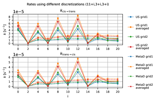
Figure S.1: Isomerization rates as a function of discretization for 3D grid-based models applied to 3D FES from metadynamics and umbrella sampling (grid3) and with averaged and position dependent diffusion for two diffusion schemes grid1 (Fig. S.10) and grid2 (Fig. S.11).

II.1.9 Three-dimensional Infrequent Metadynamics

Three-dimensional infrequent metadynamics were run for both trans-cis and cis-trans transitions in sets of 30 runs for each. Biasing was done using three-dimensional Gaussians of height $0.75\,\mathrm{kJ/mol}$ with a standard deviation of $0.07\,\mathrm{rad}$ in all three dimensions, that is, along $\varphi$, $\chi_{1}$ and $\chi_{2}$. The deposition pace was $20\,\mathrm{ps}$ while a bias factor of 20 was used. Determining the biased transition time for trans-to-cis and cis-to-trans simulation was done based on the $\varphi$ value alone in the same way as for one-dimensional infrequent metadynamics described above.

The reweighted transition times were fitted to a Poisson distribution and a KS test was done using a million randomly generated points according to the TCDF from the corresponding fits, as described in Ref. 36. The corresponding rates can be found in Table LABEL:main-tab:rates. Average transition times, standard errors, Poisson fitted transition times and corresponding $p$-values can be found in Table S.5.

InMetaD
biased CV	trans$\rightarrow$cis			cis$\rightarrow$trans
	$\mu\pm\mathrm{S.E.}$ [s]	$\tau$ [s]	$p$-value	$\mu\pm\mathrm{S.E.}$ [s]	$\tau$ [s]	$p$-value
$\varphi$	$4.45\times 10^{4}\pm 7.70\times 10^{3}$	$4.58\times 10^{4}$	$0.95$	$4.16\times 10^{4}\pm 6.39\times 10^{3}$	$4.48\times 10^{4}$	$0.74$
$\varphi$, $\chi_{1}$, $\chi_{2}$	$4.06\times 10^{4}\pm 6.07\times 10^{3}$	$4.51\times 10^{4}$	$0.52$	$4.27\times 10^{4}\pm 8.98\times 10^{3}$	$3.85\times 10^{4}$	$0.98$

Table S.5: Average transition times ($\mu$), corresponding standard errors (S.E.) and transition times from Poisson fit ($\tau$) from infrequent metadynamics for classical model system with 1D biasing using $\varphi$ as collective variable and with 3D biasing in the CV space spanned by $\varphi$, $\chi_{1}$ and $\chi_{2}$. Rates mentioned in Table LABEL:main-tab:rates correspond to $1/\tau$.

III Additional tables and figures

method	equation	Moderate friction		High friction
		Small barrier
		$k_{AB}$ [ps-1]	$k_{BA}$ [ps-1]	$k_{AB}$ [ps-1]	$k_{BA}$ [ps-1]
Simple TST	(LABEL:main-eq:simpleTST)	$1.86\times 10^{-2}$	$1.94\times 10^{-2}$	$1.86\times 10^{-2}$	$1.94\times 10^{-2}$
Kramers (weak friction)	(LABEL:main-eq:KramersWeakLimit)	$6.55\times 10^{-2}$	$3.53\times 10^{-2}$	$2.09\times 10^{-1}$	$1.13\times 10^{-1}$
Kramers (moderate friction)	(LABEL:main-eq:KramersModerate)	$1.44\times 10^{-2}$	$6.77\times 10^{-3}$	$8.84\times 10^{-3}$	$4.13\times 10^{-3}$
Kramers (high friction)	(LABEL:main-eq:KramersHigh)	$3.11\times 10^{-2}$	$1.48\times 10^{-2}$	$9.73\times 10^{-3}$	$4.63\times 10^{-3}$
Grid-based	(LABEL:main-eq:Qij_SqRA_1)	$3.03\times 10^{-2}$	$1.43\times 10^{-2}$	$9.47\times 10^{-3}$	$4.49\times 10^{-3}$
Direct simulation		$1.48\times 10^{-2}$ $\pm$ $1.53\times 10^{-2}$	$6.52\times 10^{-3}$ $\pm$ $6.59\times 10^{-3}$	$1.05\times 10^{-2}$ $\pm$ $9.72\times 10^{-3}$	$5.04\times 10^{-3}$ $\pm$ $4.95\times 10^{-3}$
		High barrier
Simple TST	(LABEL:main-eq:simpleTST)	$4.58\times 10^{-9}$	$4.63\times 10^{-9}$	$4.58\times 10^{-9}$	$4.63\times 10^{-9}$
Kramers (weak friction)	(LABEL:main-eq:KramersWeakLimit)	$7.10\times 10^{-9}$	$3.32\times 10^{-9}$	$4.26\times 10^{-7}$	$1.99\times 10^{-7}$
Kramers (moderate friction)	(LABEL:main-eq:KramersModerate)	$4.47\times 10^{-9}$	$2.02\times 10^{-9}$	$1.40\times 10^{-9}$	$6.38\times 10^{-10}$
Kramers (high friction)	(LABEL:main-eq:KramersHigh)	$9.33\times 10^{-8}$	$4.22\times 10^{-8}$	$1.55\times 10^{-9}$	$7.04\times 10^{-10}$
Grid-based	(LABEL:main-eq:Qij_SqRA_1)	$8.40\times 10^{-8}$	$3.80\times 10^{-8}$	$1.40\times 10^{-9}$	$6.34\times 10^{-10}$
Infrequent metadynamics	(LABEL:main-eq:InMetaD)	$4.60\times 10^{-9}$ $\pm$ $4.26\times 10^{-9}$	$1.84\times 10^{-9}$ $\pm$ $1.37\times 10^{-9}$	$1.24\times 10^{-9}$ $\pm$ $4.05\times 10^{-10}$	$6.29\times 10^{-10}$ $\pm$ $6.72\times 10^{-10}$
		Interpolated potential
Simple TST	(LABEL:main-eq:simpleTST)	$6.08\times 10^{-13}$	$1.58\times 10^{-13}$	$6.08\times 10^{-13}$	$1.58\times 10^{-13}$
Kramers (weak friction)	(LABEL:main-eq:KramersWeakLimit)	$1.47\times 10^{-12}$	$4.11\times 10^{-13}$	$5.91\times 10^{-11}$	$1.64\times 10^{-11}$
Kramers (moderate friction)	(LABEL:main-eq:KramersModerate)	$5.92\times 10^{-13}$	$1.55\times 10^{-13}$	$2.46\times 10^{-13}$	$6.59\times 10^{-14}$
Kramers (high friction)	(LABEL:main-eq:KramersHigh)	$9.31\times 10^{-12}$	$2.20\times 10^{-12}$	$2.32\times 10^{-13}$	$5.50\times 10^{-14}$
Grid-based	(LABEL:main-eq:Qij_SqRA_1)	$1.17\times 10^{-11}$	$3.18\times 10^{-12}$	$2.94\times 10^{-13}$	$7.95\times 10^{-14}$
Infrequent metadynamics	(LABEL:main-eq:InMetaD)	$5.21\times 10^{-13}$ $\pm$ $6.39\times 10^{-13}$	$1.76\times 10^{-13}$ $\pm$ $2.18\times 10^{-13}$	$2.07\times 10^{-13}$ $\pm$ $1.98\times 10^{-13}$	$5.28\times 10^{-14}$ $\pm$ $4.95\times 10^{-14}$

Table S.6: One-dimensional potential. Kinetic rates estimated at specific friction values: $\xi=2.5\,\mathrm{ps}^{-1}$ (moderate friction - small barrier); $\xi=8\,\mathrm{ps}^{-1}$ (high friction - small barrier); $\xi=0.5\,\mathrm{ps}^{-1}$ (moderate friction - high barrier); $\xi=30\,\mathrm{ps}^{-1}$ (high friction - high barrier); $\xi=2.5\,\mathrm{ps}^{-1}$ (moderate friction - interpolated potential); $\xi=100\,\mathrm{ps}^{-1}$ (high friction - interpolated potential).

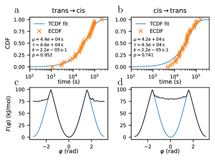
Figure S.2: a, b: TCDF fit to results of 30 InMetaD runs for trans-cis (a) and cis-trans (b) transitions. $\mu$ is the transition time averaged over 30 runs, $\tau$ is the transition time as obtained from fitting and $k=1/\tau$ the corresponding rate. $p$ is the calculated $p$-value of the KS test. c, d: Free energy profiles obtained from metadynamics simulation (as in Fig. LABEL:main-fig:FES_phi) with the biasing potential at the moment of transitioning for an example run of InMetaD for trans-cis (c) and cis-trans (d) isomerization added on top in black.

III.1 Optimized reaction coordinate

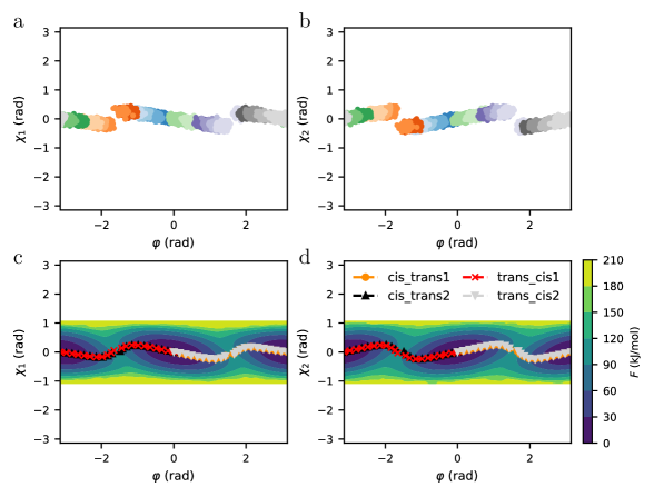
Figure S.3: Unscaled version of Fig. LABEL:main-fig:2D_correlations_FES_paths to indicate how small the out of plane bending of the improper dihedral substituents really are.

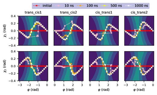
Figure S.4: Time evolution of 21 nodes of path collective variables for four trajectories of $1\,\mu\mathrm{s}$ of metadynamics, each trajectory representing one transition: cis_trans1, cis_trans2, trans_cis1 and trans_cis2. Top row: path evolution represented in 2D space spanned by $\varphi$ and $\chi_{1}$. Underlying contour plot taken from 2D-reweighted free energy surface from 3D metadynamics simulation (see also Fig. LABEL:main-fig:2D_correlations_FES_paths left). Bottom row: path evolution represented in 2D space spanned by $\varphi$ and $\chi_{2}$. Underlying contour plot taken from 2D-reweighted free energy surface from 3D metadynamics simulation (see also Fig. LABEL:main-fig:2D_correlations_FES_paths right).

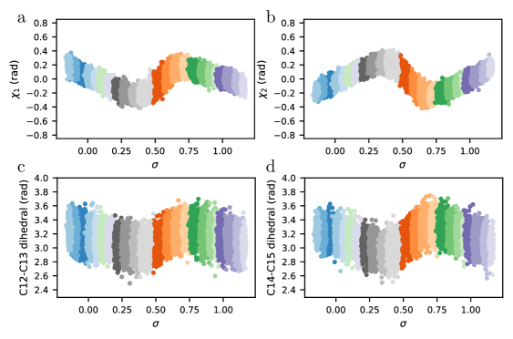
Figure S.5: a, b, c, d: Scatter plot of improper dihedrals $\chi_{1}$ (a) and $\chi_{2}$ (b) as well as proper dihedrals C₁₃=C₁₄-C₁₅=NH (c) and C₁₁=C₁₂-C₁₃=C₁₄ (d) versus the path CV for umbrella sampling along the path CV of path cis_trans1. Clearly the correlation of the improper dihedrals $\chi_{1}$ and $\chi_{2}$ is handled more smoothly as the sampling doesn’t ‘jump’ at the peaks anymore (compare to Fig. LABEL:main-fig:2D_correlations_FES_paths above). Interestingly, also the correlation of the proper dihedrals (C₁₄-C₁₅ and C₁₂-C₁₃) is handled more smoothly as the sampling doesn’t ‘jump’ at the peaks anymore either (compare to Fig. S.9 immediately above).

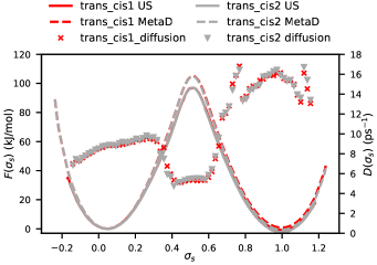
Figure S.6: Free energy profiles from metadynamics and umbrella sampling as well as diffusion profiles for optimized trans to cis path collective variable.

III.2 Umbrella sampling vs. metadynamics

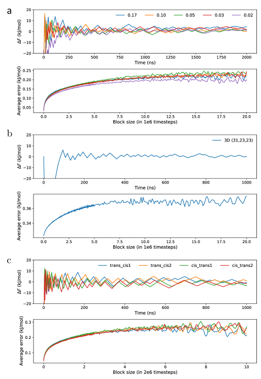
Figure S.7: Convergence of the metadynamics bias Convergence of free energy difference between trans and cis for metadynamics bias and error convergence from block analysis for: a: MetaD simulations biasing the C₁₃=C₁₄ dihedral angle $\varphi$ for different Gaussian standard deviations (in radians). All these simulations were run for $2\,\mathrm{\mu s}$ with a deposition pace of $1\,\mathrm{ps}$ and a biasing factor of 10. b: 3D MetaD simulation. Error convergence from block analysis for 3D free energy surface was done using discretization (31,23,23). Simulation was run for $1\,\mathrm{\mu s}$ with a deposition pace of $1\,\mathrm{ps}$ and a biasing factor of 12. c: MetaD simulations along path CVs. Simulation was run for $1\,\mathrm{\mu s}$ with a deposition pace of $0.5\,\mathrm{ps}$ and a biasing factor of 12.

Convergence of the free energy difference between the cis and trans state $\Delta F=F_{\mathrm{cis}}-F_{\mathrm{trans}}$ in the metadynamics biases are given in Fig. S.7 for different metadynamics runs. For the corresponding details about parameter sets, see SI section II.1. For the final free energy surfaces, see Figs. LABEL:main-fig:FES_phi and LABEL:main-fig:2D_correlations_FES_paths.

The free energy difference at a certain simulation time is calculated by determining the FES corresponding to the bias at that time (i.e. from the scaled upside-down bias, see Refs. 22, 27, 25). This FES is used to calculate the relative probabilities of being in cis versus being in trans. Using Eq. S3:

$$\pi_{\mathrm{cis}}=\int_{-\pi/2}^{\pi/2}\mathrm{d}\varphi\,\pi(\varphi)=\int_{-\pi/2}^{\pi/2}\mathrm{d}\varphi\,\exp\left(-\frac{F(\varphi)}{RT}\right)$$ (S33)

and equivalent for trans in $\varphi<-\pi/2$ and $\varphi>\pi/2$. For the 3D FES, the integration is additionally carried out over $\chi_{1}$ and $\chi_{2}$ over their full range. The free energy of a state can then be calculated using $F_{\mathrm{cis}}=-RT\ln\pi_{\mathrm{cis}}$ and equivalent for trans, and the free energy difference

$$\Delta F=F_{\mathrm{cis}}-F_{\mathrm{trans}}=-RT\ln\frac{\pi_{\mathrm{cis}}}{\pi_{\mathrm{trans}}}\,.$$ (S34)

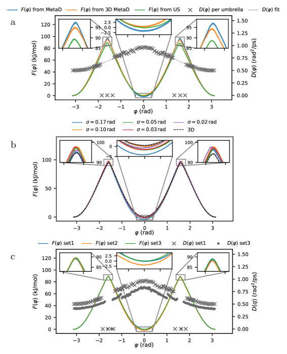
Figure S.8: a: Free energy surfaces $F(\varphi)$ and diffusion profiles $D(\varphi)$ estimated from MetaD and US biasing C₁₃=C₁₄ torsion angle $\varphi$ including standard errors.
b: Free energy profiles for metadynamics simulations biasing the C₁₃=C₁₄ dihedral angle $\varphi$ for different Gaussian standard deviations (in radians), as well as profile reweighted from 3D metadynamics. One-dimensional metadynamics simulations (colored) were run for $2\,\mathrm{\mu s}$ with a deposition pace of $1\,\mathrm{ps}$ using Gaussians with a height of $1.2\,\mathrm{kJ/mol}$ and a biasing factor of 10. 3D metadynamics simulation (black, dashed) was run for $1\,\mathrm{\mu s}$ with a deposition pace of $1\,\mathrm{ps}$ using Gaussians with a height of $1.2\,\mathrm{kJ/mol}$ and a width of $0.07\,\mathrm{rad}$ in each dimension and a biasing factor of 12.
c: Free energy profiles for US simulations biasing the C₁₃=C₁₄ dihedral angle $\varphi$. The statistical uncertainty of the free energy profiles are shown as shaded areas, but they are so small, that they are hardly discernible.

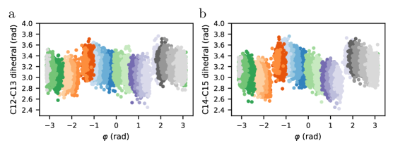
Figure S.9: a, b: Scatter plot of proper dihedrals C₁₃=C₁₄-C₁₅=NH (a) and C₁₁=C₁₂-C₁₃=C₁₄ (b) versus $\varphi$ for umbrella sampling along $\varphi$ (US set2). These proper dihedrals are also correlated and also cause hysteresis when using $\varphi$ as a reaction coordinate (compare to Fig. LABEL:main-fig:2D_correlations_FES_paths above).

III.3 Multidimensional models

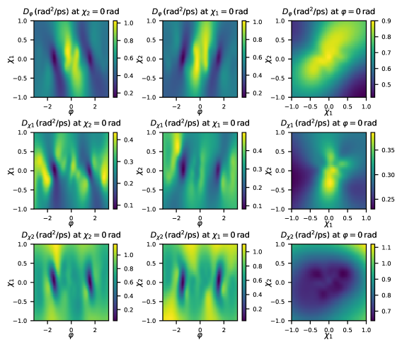
Figure S.10: Interpolated three-dimensional diffusion surfaces $D_{\varphi}$, $D_{\chi_{1}}$ and $D_{\chi_{2}}$ obtained from grid1 of three-dimensional harmonic restraints.

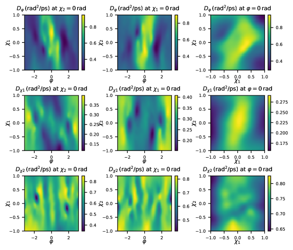
Figure S.11: Interpolated three-dimensional diffusion surfaces $D_{\varphi}$, $D_{\chi_{1}}$ and $D_{\chi_{2}}$ obtained from grid2 of three-dimensional harmonic restraints.

IV References

References

- [1] Hannes Risken and Hannes Risken. Fokker-Planck equation. Springer, 1996.
- [2] J. A . Izaguirre, C. R. Schweet, and V.S. Pande. Multiscale dynamics of macromolecules using normal mode Langevin. Pacific Symposium on Biocomputing, 15:240–251, 2010.
- [3] Peter Hänggi, Peter Talkner, and Michal Borkovec. Reaction-rate theory: fifty years after kramers. Rev. Mod. Phys., 62:251–341, 1990.
- [4] Baron Peters. Reaction Rate Theory and Rare Events. Elsevier, 1st edition, 2017.
- [5] H Pelzer and E Wigner. The speed constansts of the exchange reactions. Z. Phys. Chem. B, 15:445–552, 1932.
- [6] George H Vineyard. Frequency factors and isotope effects in solid state rate processes. Journal of Physics and Chemistry of Solids, 3(1-2):121–127, 1957.
- [7] Emadeddin Tajkhorshid, Béla Paizs, and Sandor Suhai. Role of isomerization barriers in the pKa control of the retinal Schiff base: a density functional study. The Journal of Physical Chemistry B, 103(21):4518–4527, 1999.
- [8] Shigehiko Hayashi, Emad Tajkhorshid, and Klaus Schulten. Structural changes during the formation of early intermediates in the bacteriorhodopsin photocycle. Biophysical Journal, 83(3):1281–1297, 2002.
- [9] Emadeddin Tajkhorshid, Jérôme Baudry, Klaus Schulten, and Sandor Suhai. Molecular dynamics study of the nature and origin of retinal’s twisted structure in bacteriorhodopsin. Biophysical Journal, 78(2):683–693, 2000.
- [10] Erik Malmerberg, Ziad Omran, Jochen S Hub, Xuewen Li, Gergely Katona, Sebastian Westenhoff, Linda C Johansson, Magnus Andersson, Marco Cammarata, Michael Wulff, et al. Time-resolved WAXS reveals accelerated conformational changes in iodoretinal-substituted proteorhodopsin. Biophysical Journal, 101(6):1345–1353, 2011.
- [11] Kresten Lindorff-Larsen, Stefano Piana, Kim Palmo, Paul Maragakis, John L Klepeis, Ron O Dror, and David E Shaw. Improved side-chain torsion potentials for the Amber ff99SB protein force field. Proteins: Structure, Function, and Bioinformatics, 78(8):1950–1958, 2010.
- [12] Oleksandr Volkov, Kirill Kovalev, Vitaly Polovinkin, Valentin Borshchevskiy, Christian Bamann, Roman Astashkin, Egor Marin, Alexander Popov, Taras Balandin, Dieter Willbold, et al. Structural insights into ion conduction by channelrhodopsin 2. Science, 358(6366), 2017.
- [13] David Van Der Spoel, Erik Lindahl, Berk Hess, Gerrit Groenhof, Alan E Mark, and Herman JC Berendsen. GROMACS: fast, flexible, and free. Journal of Computational Chemistry, 26(16):1701–1718, 2005.
- [14] Mark James Abraham, Teemu Murtola, Roland Schulz, Szilárd Páll, Jeremy C Smith, Berk Hess, and Erik Lindahl. GROMACS: High performance molecular simulations through multi-level parallelism from laptops to supercomputers. SoftwareX, 1:19–25, 2015.
- [15] Wikipedia. Dihedral angle — Wikipedia, The Free Encyclopedia. http://en.wikipedia.org/w/index.php?title=Dihedral%20angle&oldid=1155191517, 2023. [Online; accessed 08-June-2023].
- [16] The PLUMED consortium. Plumed2. https://github.com/plumed/plumed2, 2019.
- [17] Wikipedia. Atan2 — Wikipedia, The Free Encyclopedia. http://en.wikipedia.org/w/index.php?title=Atan2&oldid=1156958741, 2023. [Online; accessed 08-June-2023].
- [18] Massimiliano Bonomi, Davide Branduardi, Giovanni Bussi, Carlo Camilloni, Davide Provasi, Paolo Raiteri, Davide Donadio, Fabrizio Marinelli, Fabio Pietrucci, Ricardo A Broglia, et al. PLUMED: A portable plugin for free-energy calculations with molecular dynamics. Computer Physics Communications, 180(10):1961–1972, 2009.
- [19] Gareth A Tribello, Massimiliano Bonomi, Davide Branduardi, Carlo Camilloni, and Giovanni Bussi. PLUMED 2: New feathers for an old bird. Computer Physics Communications, 185(2):604–613, 2014.
- [20] The PLUMED consortium. Promoting transparency and reproducibility in enhanced molecular simulations. Nature Methods, 16(8):670–673, 2019.
- [21] Alessandro Barducci, Giovanni Bussi, and Michele Parrinello. Well-tempered metadynamics: a smoothly converging and tunable free-energy method. Physical Review Letters, 100(2):020603, 2008.
- [22] Davide Branduardi, Giovanni Bussi, and Michele Parrinello. Metadynamics with adaptive Gaussians. Journal of Chemical Theory and Computation, 8(7):2247–2254, 2012.
- [23] Massimiliano Bonomi, Alessandro Barducci, and Michele Parrinello. Reconstructing the equilibrium Boltzmann distribution from well-tempered metadynamics. Journal of Computational Chemistry, 30(11):1615–1621, 2009.
- [24] Pratyush Tiwary and Michele Parrinello. A time-independent free energy estimator for metadynamics. The Journal of Physical Chemistry B, 119(3):736–742, 2015.
- [25] Giovanni Bussi and Alessandro Laio. Using metadynamics to explore complex free-energy landscapes. Nature Reviews Physics, 2(4):200–212, 2020.
- [26] Jérôme Hénin, Tony Lelièvre, Michael R Shirts, Omar Valsson, and Lucie Delemotte. Enhanced sampling methods for molecular dynamics simulations. arXiv preprint arXiv:2202.04164, 2022.
- [27] Giovanni Bussi and Gareth A Tribello. Analyzing and biasing simulations with PLUMED. In Biomolecular Simulations, pages 529–578. Springer, 2019.
- [28] Zhiqiang Tan, Emilio Gallicchio, Mauro Lapelosa, and Ronald M Levy. Theory of binless multi-state free energy estimation with applications to protein-ligand binding. The Journal of Chemical Physics, 136(14):04B608, 2012.
- [29] Gerhard Hummer. Position-dependent diffusion coefficients and free energies from Bayesian analysis of equilibrium and replica molecular dynamics simulations. New Journal of Physics, 7(1):34, 2005.
- [30] Bradley Efron. The jackknife, the bootstrap and other resampling plans. SIAM, 1982.
- [31] Donald F Gatz and Luther Smith. The standard error of a weighted mean concentration—-I. Bootstrapping vs other methods. Atmospheric Environment, 29(11):1185–1193, 1995.
- [32] Jochen S Hub, Bert L De Groot, and David Van Der Spoel. g_wham a free weighted histogram analysis implementation including robust error and autocorrelation estimates. Journal of Chemical Theory and Computation, 6(12):3713–3720, 2010.
- [33] Jan O Daldrop, Julian Kappler, Florian N Brünig, and Roland R Netz. Butane dihedral angle dynamics in water is dominated by internal friction. Proceedings of the National Academy of Sciences, 115(20):5169–5174, 2018.
- [34] Fredrik Johansson. mpmath. https://github.com/fredrik-johansson/mpmath.
- [35] Fredrik Johansson. python-flint. https://github.com/fredrik-johansson/python-flint.
- [36] Matteo Salvalaglio, Pratyush Tiwary, and Michele Parrinello. Assessing the reliability of the dynamics reconstructed from metadynamics. Journal of Chemical Theory and Computation, 10(4):1420–1425, 2014.
- [37] Grisell Díaz Leines and Bernd Ensing. Path finding on high-dimensional free energy landscapes. Physical Review Letters, 109(2):020601, 2012.
- [38] Alberto Pérez de Alba Ortíz, Jocelyne Vreede, and Bernd Ensing. The adaptive path collective variable: a versatile biasing approach to compute the average transition path and free energy of molecular transitions. In Biomolecular Simulations, pages 255–290. Springer, 2019.
- [39] Alberto Pérez de Alba Ortíz and Bernd Ensing. Simultaneous sampling of multiple transition channels using adaptive paths of collective variables. arXiv preprint arXiv:2112.04061, 2021.