Robust Loss Functions for Training Decision Trees with Noisy Labels

Abstract

We consider training decision trees using noisily labeled data, focusing on loss functions that can lead to robust learning algorithms. Our contributions are threefold. First, we offer novel theoretical insights on the robustness of many existing loss functions in the context of decision tree learning. We show that some of the losses belong to a class of what we call conservative losses, and the conservative losses lead to an early stopping behavior during training and noise-tolerant predictions during testing. Second, we introduce a framework for constructing robust loss functions, called distribution losses. These losses apply percentile-based penalties based on an assumed margin distribution, and they naturally allow adapting to different noise rates via a robustness parameter. In particular, we introduce a new loss called the negative exponential loss, which leads to an efficient greedy impurity-reduction learning algorithm. Lastly, our experiments on multiple datasets and noise settings validate our theoretical insight and the effectiveness of our adaptive negative exponential loss.

Introduction

Noisily labeled data often arise in machine learning, due to reasons such as the difficulty of accurately labeling data and the use of crowd-sourcing for labeling (Song et al. 2022). Various approaches have been developed to handle the label noise, including eliminating mislabeled examples (Brodley, Friedl et al. 1996), implicit/explicit regularization (Tanno et al. 2019; Lukasik et al. 2020), the use of robust loss functions (Manwani and Sastry 2013; Yang, Gao, and Li 2019), with recent works mostly focusing on neural networks.

This paper focuses on robust loss functions for learning decision trees from noisily labeled data. Tree-based methods (e.g., random forests) are among the most effective machine learning methods, particularly on tabular data (Grinsztajn, Oyallon, and Varoquaux 2022; Kaggle 2021), and several robust loss functions have been shown to be effective for neural network learning in the presence of label noise (e.g., see (Ghosh, Kumar, and Sastry 2017; Zhang and Sabuncu 2018)). However, little attention has been paid to the understanding and design of robust loss functions in the context of decision tree learning. This is likely because decision tree learning algorithms are often described as greedy impurity-reduction algorithms in the literature, and it is less well-known that the impurity-reduction algorithms are greedy algorithms for minimizing certain losses (Yang, Gao, and Li 2019; Wilton et al. 2022). Our work aims to address this research gap.

Our main contributions are three-fold.

• We offer novel theoretical insight on the robustness of many existing loss functions. We show that some of them belong to a class of what we call conservative losses, which are robust due to an early stopping behavior during training and noise-tolerant predictions during testing.

• We introduce a framework for constructing robust loss functions, called distribution losses. These losses apply percentile-based penalties based on an assumed margin distribution. By using different assumed margin distributions, we can recover some commonly used loss functions, which shed interesting insight on these existing functions. An attractive property of the distribution loss is that they naturally allow adapting to different noise rates via a robustness parameter. Importantly, we introduce a new loss called the negative exponential loss, which leads to an efficient impurity-reduction learning algorithm.

• Our extensive experiments validate our theoretical insight and the effectiveness of our adaptive negative exponential loss.

The remainder of this paper is organized as follows. We first provide a more detailed discussion on related work, followed by some preliminary concepts. We then present the conservative losses and their robustness properties. After that, we describe our distribution-based robust loss framework and the negative exponential loss. Finally, we present details on experimental settings and results, with a brief conclusion. Our source code is available at https://github.com/jonathanwilton/RobustDecisionTrees.

Related Work

Our work is broadly related to the large body of approaches developed for dealing with label noise in the literature, which include filtering the noisy labels, learning a classifier and model for the label noise simultaneously, implicit/explicit regularization to avoid overfitting the noise, and designing robust loss functions (see, e.g., for the excellent reviews (Frénay and Verleysen 2013) or (Song et al. 2022) for detailed discussions).

The most relevant general approach to our work is the robust loss approach. There are two common approaches to design robust losses. One creates corrected losses by incorporating label noise rates if they are known (e.g., see (Natarajan et al. 2013; Patrini et al. 2017)). However, such information is typically unknown, and difficult to estimate accurately in practice. Another approach considers inherently robust losses, which does not require knowledge of the noise rates. Some pioneering theoretical works consider robustness of losses against label noise (Manwani and Sastry 2013; Ghosh, Manwani, and Sastry 2015; Ghosh, Kumar, and Sastry 2017). These works show that the zero-one (01) loss and mean absolute error (MAE) are robust to many types of label noise, while the commonly used cross entropy (CE) loss does not enjoy these same robustness properties. This sparked interest in developing new loss functions that share favorable qualities from each of the 01, MAE and CE, for example the generalized cross entropy (GCE) loss (Zhang and Sabuncu 2018), negative learning (Kim et al. 2019), symmetric cross entropy loss (Wang et al. 2019), curriculum loss (Lyu and Tsang 2020) and normalized loss functions (Ma et al. 2020). However, losses like the curriculum loss and the normalized losses are not suitable for decision tree learning, because the impurities for these losses lack analytical forms and efficient algorithms.

Our work is also closely related to tree methods for learning from noisily labeled data. Motivated by the predictive performance and interpretability of tree methods (Breiman et al. 1984; Breiman 2001; Geurts, Ernst, and Wehenkel 2006), various works have developed algorithms for decision tree learning in the presence of label noise, such as pruning (Breiman et al. 1984), making use of pseudo-examples during tree construction (Mantas and Abellan 2014), leaving a large number of samples at each leaf node (Ghosh, Manwani, and Sastry 2017), and adjusting the labels at each leaf node of a trained RF (Zhou, Ding, and Li 2019). To the best of our knowledge, the closest work to ours derives a robust impurity from the well-known ranking loss (Yang, Gao, and Li 2019). They only consider binary classification and their approach does not adapt to the noise rate, while we also consider multiclass classification and our approach adapts to the underlying noise rate. In addition, we offer novel theoretical insight on the robustness of various existing losses, and we contribute a general framework for constructing robust losses.

Preliminaries

Learning With Noisy Labels

We consider $K$-class classification problem, where the input ${\bm{x}}\in{\mathbb{R}}^{d}$ and the one-hot label ${\bm{y}}\in\{0,1\}^{K}$ follows a joint distribution $p({\bm{x}},{\bm{y}})$. In the standard noise-free setting, we are given a training set ${\cal{D}}=\{({\bm{x}}_{i},{\bm{y}}_{i})\}_{i=1}^{n}$ consisting of examples independently sampled from $p({\bm{x}},{\bm{y}})$. In the noisy setting, we have a dataset $\widetilde{{\cal{D}}}=\{({\bm{x}}_{i},\widetilde{{\bm{y}}}_{i})\}_{i=1}^{n}$ where each noisy label $\widetilde{{\bm{y}}}$ is obtained by randomly flipping the true label ${\bm{y}}$ with probability $\eta_{jk}^{{\bm{x}}}:={\mathbb{P}}(\widetilde{{\bm{y}}}={\bm{e}}_{k}\,|\,{\bm{y}}={\bm{e}}_{j},{\bm{x}})$, with ${\bm{e}}_{j}$ being the one-hot vector for class $j$. We focus on class-conditional noise, where the noise probability is independent of the input, that is, each $\eta_{jk}^{{\bm{x}}}$ is equal to some constant $\eta_{jk}$ for all ${\bm{x}}$. In particular, we consider the special case of uniform noise, in which each class has the same corruption rates, that is, $\eta_{jk}=1-\eta$ for $j=k$ and $\eta_{jk}=\eta/(K-1)$ for $j\neq k$, for some constant $\eta$.

The objective is to learn a classifier ${\bm{g}}:{\mathbb{R}}^{d}\to\Delta$ to minimize the expected risk

$$R({\bm{g}}):={\mathbb{E}}_{({\bm{x}},{\bm{y}})\sim p({\bm{x}},{\bm{y}})}\,\ell({\bm{g}}({\bm{x}}),{\bm{y}}),$$

where $\ell:{\mathbb{R}}^{K}\times{\mathbb{R}}^{K}\to{\mathbb{R}}$ is a loss function, and $\Delta=\{{\bm{y}}\in[0,1]^{K}\,:\,{\bm{y}}^{\mathsf{T}}\bm{1}=1\}$ the standard $(K-1)$-simplex. Predicted labels can be obtained from the classifier with ${\bm{e}}_{\mathrm{argmax}({\bm{g}}({\bm{x}}))}$. With a set of noise-free training data, the risk can be estimated without bias via the empirical risk

$$\widehat{R}({\bm{g}};{\cal{D}}):=\sum_{({\bm{x}},{\bm{y}})\in{\cal{D}}}\ell({\bm{g}}({\bm{x}}),{\bm{y}})/|{\cal{D}}|.$$

When only a noisily labeled dataset $\widetilde{{\cal{D}}}$ is available, we instead estimate the expected risk with $\widehat{R}({\bm{g}};\widetilde{{\cal{D}}})$.

We focus on loss functions that are robust against label noise. A loss function $\ell$ is said to be noise tolerant if the minimizers of the expected risk using loss $\ell$ on the noisy and noise-free data distributions lead to the same expected risk using the 01 loss on noise-free data (Manwani and Sastry 2013). If a loss function $\ell$ is symmetric, i.e., $\sum_{j=1}^{K}\ell({\bm{g}}({\bm{x}}),{\bm{e}}_{j})=C$ for any ${\bm{x}}\in{\mathbb{R}}^{d}$ and any ${\bm{g}}$, then, under uniform label noise with $\eta<\frac{K-1}{K}$, $\ell$ is noise tolerant (Ghosh, Manwani, and Sastry 2015; Ghosh, Kumar, and Sastry 2017). If we additionally have $R({\bm{g}}^{*})=0$ for some classifier ${\bm{g}}^{*}$, $0\leq\ell({\bm{g}}({\bm{x}}),{\bm{e}}_{j})\leq C/(K-1)\,\forall j=1,\ldots,K$ and the matrix $(\eta_{ij})_{i,j=1}^{K}$ is diagonally dominant, then $\ell$ is noise tolerant under class conditional noise (Ghosh, Kumar, and Sastry 2017). Examples of symmetric loss functions include the $01$ loss $\ell(\widehat{{\bm{y}}},{\bm{e}}_{j})=\mathds{1}(\widehat{{\bm{y}}}\neq{\bm{e}}_{j})$ and MAE loss $\ell(\widehat{{\bm{y}}},{\bm{e}}_{j})=\|\widehat{{\bm{y}}}-{\bm{e}}_{j}\|_{1}$. On the other hand, the mean squared error (MSE) loss $\ell(\widehat{{\bm{y}}},{\bm{e}}_{j})=\|\widehat{{\bm{y}}}-{\bm{e}}_{j}\|_{2}^{2}$ and CE loss $\ell(\widehat{{\bm{y}}},{\bm{e}}_{j})=-{\bm{e}}_{j}^{\mathsf{T}}\log\widehat{{\bm{y}}}$ are not symmetric. In practice it has been shown that training neural network (NN) classifiers with these noise tolerant loss functions can lead to significantly longer training time before convergence (Zhang and Sabuncu 2018). The GCE loss $\ell(\widehat{{\bm{y}}},{\bm{e}}_{j})=(1-({\bm{e}}_{j}^{\mathsf{T}}\widehat{{\bm{y}}})^{q})/q$ was proposed as a compromise between noise-robustness and good performance (Zhang and Sabuncu 2018). The hyperparameter $q\in[0,1]$ controls the robustness, with special cases $q=0$ giving the CE and $q=1$ the MAE.

Decision Tree Learning

We briefly review two dual perspectives for decision tree learning: learning by impurity reduction, and learning by recursive greedy risk minimization.

In the impurity reduction perspective, the decision tree construction process recursively partitions the (possibly noisy) training set ${\cal{D}}$ such that each subset has similar labels. We start with a single node associated with the entire training set. Each time we have a node associated with a subset ${\cal{S}}\subseteq{\cal{D}}$ that we need to split, we find an optimal split $(f,t)$ that partitions ${\cal{S}}$ into ${\cal{S}}_{f\leq t}$ and ${\cal{S}}_{f>t}$ based on whether the feature $f$ is larger than the value $t$. The quality of a split is usually measured by its reduction in some label impurity measure $I$, defined by:

$$\frac{|{\cal{S}}|}{|{\cal{D}}|}I({\cal{S}})-\frac{|{\cal{S}}_{f\leq t}|}{|{\cal{D}}|}I({\cal{S}}_{f\leq t})-\frac{|{\cal{S}}_{f>t}|}{|{\cal{D}}|}I({\cal{S}}_{f>t}).$$

Based on the split, two child nodes associated with ${\cal{S}}_{f\leq t}$ and ${\cal{S}}_{f>t}$ are created. This process is repeated recursively on the two child nodes until some stopping criteria is satisfied.

In the recursive greedy risk minimization perspective, a node is split in a greedy way to minimize the empirical risk $\widehat{R}({\bm{g}};{\cal{D}})$. If ${\bm{g}}$ predicts a constant $\widehat{{\bm{y}}}$ on a subset ${\cal{S}}\subseteq{\cal{D}}$ of the training examples, then the contribution to the empirical risk is the partial empirical risk $\widehat{R}(\widehat{{\bm{y}}};{\cal{S}}):=\sum_{({\bm{x}},{\bm{y}})\in{\cal{S}}}\ell(\widehat{{\bm{y}}},{\bm{y}})/|{\cal{D}}|.$ Denote by $\widehat{{\bm{y}}}^{*}:=\mathrm{argmin}_{\widehat{{\bm{y}}}\in\Delta}\widehat{R}(\widehat{{\bm{y}}};{\cal{S}})$ the optimal constant probability vector prediction, with minimum partial empirical risk

$$\widehat{R}^{*}({\cal{S}}):=\widehat{R}(\widehat{{\bm{y}}}^{*};{\cal{S}}).$$

The minimum partial empirical risk can be interpreted as an impurity measure. In fact, it is the Gini impurity and the entropy impurity (up to a multiplicative constant) when the loss is the MSE loss and the CE loss, respectively.

If we switch from a constant prediction rule to a decision stump that splits on feature $f$ at threshold $t$, then the minimum partial empirical risk for the decision stump is $\widehat{R}^{*}({\cal{S}}_{f\leq t})+\widehat{R}^{*}({\cal{S}}_{f>t})$, and the risk reduction for the split $(f,t)$ is

$${\rm RR}(f,t;{\cal{S}}):=\widehat{R}^{*}({\cal{S}})-\widehat{R}^{*}({\cal{S}}_{f\leq t})-\widehat{R}^{*}({\cal{S}}_{f>t}).$$ (1)

We will use a subscript to specify the loss if needed. For example, $\widehat{R}_{\mathrm{MSE}}^{*}({\cal{S}})$ and ${\rm RR}_{\mathrm{MSE}}(f,t;{\cal{S}})$ indicates that the MSE loss is used for computing the minimum partial empirical risk and the risk reduction for a split $(f,t)$ on ${\cal{S}}$, respectively.

The equivalence between loss functions and impurity measures has been explored in, for example, (Yang, Gao, and Li 2019; Wilton et al. 2022). To illustrate, let ${\bm{p}}$ be the empirical class distribution for ${\cal{S}}$. Then the minimum partial risks for MSE and CE are the commonly used Gini impurity $1-\|{\bm{p}}\|_{2}^{2}$ and entropy impurity $-{\bm{p}}^{\mathsf{T}}\log{\bm{p}}$, respectively, up to a multiplicative constant (see (a) and (b) of Theorem 1). Note that not all loss functions have impurities which have analytical forms and efficient algorithms, while our negative exponential loss yields an impurity which has an efficiently computable analytical formula, which is important for efficient decision tree learning.

For prediction, each test example is assigned to a leaf node based on its feature values, then labeled according to the majority label of the examples at the leaf node. Generalization performance of the decision tree classifier can be measured by comparing predictions on unseen data with true labels, however, it can be heavily affected when training data, particularly labels, are unreliable.

Conservative Losses

We first examine the impurities corresponding to various loss functions, including both standard loss functions and robust ones, in Theorem 1. Parts $(a)$, $(b)$ and $(c)$ are shown in previous works (Breiman et al. 1984; Painsky and Wornell 2018; Yang, Gao, and Li 2019; Wilton et al. 2022) but included for completeness. All proofs are given in the appendices. Unless otherwise stated, we shall use ${\cal{D}}$ to denote an arbitrary (possibly noisy) set of input-output pairs, and ${\cal{S}}$ a subset of ${\cal{D}}$, in this section.

Theorem 1.

Let $W_{{\cal{S}}}=|{\cal{S}}|/|{\cal{D}}|$ and ${\bm{p}}=(p_{1},\ldots,p_{K})^{\mathsf{T}}\in\Delta$ be the empirical class probability vector for ${\cal{S}}$, that is, $p_{j}=\sum_{({\bm{x}},{\bm{y}})\in{\cal{S}}}\mathds{1}({\bm{y}}={\bm{e}}_{j})/|{\cal{S}}|,\forall j=1,\ldots,K$. Then,

1. $\widehat{R}_{\mathrm{MSE}}^{*}({\cal{S}})=W_{{\cal{S}}}(1-\|{\bm{p}}\|_{2}^{2})$,

2. $\widehat{R}_{\mathrm{CE}}^{*}({\cal{S}})=W_{{\cal{S}}}(-{\bm{p}}^{\mathsf{T}}\log{\bm{p}})$,

3. $\widehat{R}_{\mathrm{01}}^{*}({\cal{S}})=W_{{\cal{S}}}(1-\|{\bm{p}}\|_{\infty})$,

4. $\widehat{R}_{\mathrm{GCE}}^{*}({\cal{S}})=\begin{cases}W_{{\cal{S}}}(-{\bm{p}}^{\mathsf{T}}\log{\bm{p}}),&q=0,\\ W_{{\cal{S}}}(1-\|{\bm{p}}\|_{1/(1-q)})/q,&\forall q\in(0,1),\\ W_{{\cal{S}}}(1-\|{\bm{p}}\|_{\infty})/q,&q\geq 1,\end{cases}$

5. $\widehat{R}_{\mathrm{MAE}}^{*}({\cal{S}})=2W_{{\cal{S}}}(1-\|{\bm{p}}\|_{\infty})$.

The result highlights an interesting observation on the impurities of two robust losses, the MAE loss and the 01 loss (Ghosh, Kumar, and Sastry 2017): both lead to the misclassification impurity $1-\|{\bm{p}}\|_{\infty}$, up to a multiplicative constant. Furthermore, the GCE is equivalent to an impurity measure that interpolates between the misclassification and entropy impurities depending on the chosen value of $q$. This is consistent with the fact that GCE interpolates between CE and MAE loss for $q\in(0,1)$ (Zhang and Sabuncu 2018).

Below, we introduce a broad class of losses that lead to the misclassification impurity, and provide a few results to justify their robustness properties in the context of decision tree learning with label noise.

Definition 1.

A loss function $\ell$ is called $C$-conservative if, for some constant $C>0$, it satisfies the following properties:

1. $\sum_{j=1}^{K}\ell(\widehat{{\bm{y}}},{\bm{e}}_{j})\geq C(K-1),\ \forall\widehat{{\bm{y}}}\in\Delta$,

2. $\ell(\widehat{{\bm{y}}},{\bm{e}}_{j})\leq C,\ \forall\widehat{{\bm{y}}}\in\Delta,\ \forall j=1,\ldots,K$, and

3. $\ell({\bm{e}}_{j},{\bm{e}}_{j})=0,\ \forall j=1,\ldots,K$.

Intuitively, (a) and (b) implies that the loss assigned to a single class is never too much as compared to the total loss assigned to all classes.

Theorem 2.

In a $K$ class classification problem let $\ell:{\mathbb{R}}^{K}\times{\mathbb{R}}^{K}\to[0,\infty)$ be a loss function, and ${\bm{p}}\in\Delta$ be the vector of proportions of examples in ${\cal{S}}$ from each class. Then, we have

$$\widehat{R}^{*}({\cal{S}}) =C{W_{\cal{S}}}(1-\|{\bm{p}}\|_{\infty})$$ (2)

if $\ell$ is $C$-conservative. In addition, if Eq. 2 holds, then $\ell$ satisfies (a) in 1.

This theorem provides a convenient way to check if a loss function leads to the misclassification impurity, as illustrated in Corollary 2.1.

Corollary 2.1.

The MAE, 01 loss, GCE $(q\geq 1)$ and infinity norm loss satisfy $\widehat{R}^{*}({\cal{S}})=W_{{\cal{S}}}\,C(1-\|{\bm{p}}\|_{\infty}),$ with $C=2,\,1,\,1/q$ and $1$, respectively.

Our first robustness property of the conservative loss is concerned with the optimal predictions.

Theorem 3.

Assume $\ell$ is a conservative loss function. Then,

$$\underset{\widehat{{\bm{y}}}\in\Delta}{\mathrm{argmin}}\,\widehat{R}(\widehat{{\bm{y}}};{\cal{S}})={\bm{e}}_{\mathrm{argmax}({\bm{p}})}.$$

Moreover, for non-conservative loss functions MSE and CE,

$$\underset{\widehat{{\bm{y}}}\in\Delta}{\mathrm{argmin}}\,\widehat{R}(\widehat{{\bm{y}}};{\cal{S}})={\bm{p}}.$$

This result suggests that the optimal constant prediction at each node is less likely to change after label corruption when the loss functions are conservative versus not. This is because for a conservative loss, the optimal constant prediction is the one-hot vector for the most likely class, which is likely to remain the same after label noise is added.

Our second robustness result, Theorem 4, provides a more precise statement on the effect of noise on the majority class. Specifically, we show that a sample size of $O(1/\gamma^{2})$ is needed to guarantee that the majority class remains the same under the label noise, where $\gamma$ is a margin parameter that depends on the noise and the class distribution of the clean dataset, as defined in the theorem below.

Theorem 4.

Let ${\cal{S}}$ be a set of $n$ noise-free examples, $p_{k}$ be the empirical probability of class $k$ in ${\cal{S}}$, and $k^{*}$ the most prevalent class in ${\cal{S}}$, that is, $p_{k^{*}}>p_{k}$ for any $k\neq k^{*}$. In addition, let $\widetilde{{\cal{S}}}$ be obtained from ${\cal{S}}$ by applying a uniform noise with rate $\eta<(K-1)/K$, and $\widetilde{p}_{k}$ the empirical probability of class $k$ in $\widetilde{{\cal{S}}}$. Then

$${\mathbb{P}}(\widetilde{p}_{k^{*}}\geq\widetilde{p}_{k}\text{ for all $k\neq k^{*}$}\,|\,{\cal{S}}) \geq 1-(K-1)e^{-n\gamma^{2}/2},$$

with $\gamma=\underset{k\neq k^{*}}{\min}\,(\widetilde{p}_{k^{*}}^{\eta}-\widetilde{p}_{k}^{\eta})$, and $\widetilde{p}_{j}^{\eta}={\mathbb{E}}[\widetilde{p}_{j}\,|\,{\cal{S}}],\ \forall\,j=1,\ldots,K$.

Our third robustness result, Theorem 5, shows that a conservative loss leads to an early stopping property that is robust against label noise, while a non-conservative loss generally does not have this property and stops under a much more stringent condition.

Theorem 5.

Assume that tree growth at a node is halted when the risk reduction at the node for any split is non-positive.

• For a conservative loss, a node will stop splitting if and only if the majority classes at the node are also the majority classes at both child nodes for all splits.

• For the MSE, CE or GCE $(q\in(0,1))$ loss, splitting is only halted if the parent node and both child nodes all share the same label distribution for all splits.

We found in our experiments that this early stopping phenomenon does indeed happen in practice, and tends to help tree methods avoid overfitting in situations with large amounts of noise in the training labels. However, we also observed that this early stopping can sometimes lead to underfitting in low noise situations, as predicted in (Breiman et al. 1984) for noise-free data. Note that we give a necessary and sufficient condition for early stopping with conservative loss functions and compare to each of the MSE, CE and GCE $(q\in(0,1))$, while a sufficient condition for early stopping with the misclassification impurity and comparison with Gini impurity can be found in (Breiman et al. 1984).

Distribution Losses

We introduce a new approach for constructing robust loss functions that can adapt to the noise level. This allows us to address a limitation of the conservative losses as pointed out in the previous section: while conservative losses are robust against label noise, they can lead to underfitting in low noise situations.

Our approach is based on a simple idea that we will use to unify various common losses. Specifically, consider binary classification, and let $y\in\{-1,1\}$, $\widehat{y}\in{\mathbb{R}}$, and $z=y\widehat{y}$ denote the true label, the prediction, and the margin, respectively, then for any CDF $F$, $\ell(y,\widehat{y})=F(-z)$ can be used as a loss function. Intuitively, assume the margin of a random example follows the distribution $F$, then the loss is the probability that the random margin is larger than a value. We call $\ell$ a distribution loss. The loss is bounded in [0, 1], converging to 0 and 1 when $z\to+\infty$ and $z\to-\infty$, respectively.

Various commonly used loss functions are distribution losses.

Lemma 6.

The distribution loss is the 01 loss $\ell(z)=(1-\mathrm{sign}(z))/2$ for the Bernoulli distribution ${\mathsf{Ber}}(0)$; the sigmoid loss $\ell(z)=1/(1+\exp(z))$ for the logistic distribution $\mathsf{Logistic}(0,1)$; and the ramp loss $\ell(z)=\max\{0,\min\{1,(1-z)/2\}\}$ for the uniform distribution $\mathsf{U}(-1,1)$.

We instantiate the distribution loss framework to create a robust loss function with a parameter that allows for adaptation to different noise levels.

Lemma 7.

For an exponential variable $X\sim\mathsf{Exp}(1)$, consider its shifted negative $Z=\mu-X$ for some $\mu\geq 0$, then the CDF of $Z$ is

$$F(z)=\min\{1,\exp(z-\mu)\},$$

and the corresponding loss function is

$$\ell(\widehat{y},y)=\min\{1,\exp(-y\widehat{y}-\mu)\}.$$

We call this loss the negative exponential (NE) loss.

The plot of the NE loss in Figure 1 reveals several robustness properties: first, the loss is capped at 1 even for large negative margins, thus preventing imposing excessively large penalty on a noisy example far from the decision boundary; second, the rapid decrease of the loss to zero helps the classifier to avoid overfitting to large positive margins; third, the robustness parameter $\mu$ allows control on the range of negative margins that should be penalized, with a large $\mu$ allowing ignoring more noisy examples with negative margins.

NE loss can be viewed as a capped and shifted variant of the standard exponential loss. While capping creates zero gradient and thus may make gradient-based learning difficult, this is not a limitation for decision tree learning as we only need to compute the impurity. Theorem 8 gives an expression for the impurity corresponding to the NE loss.

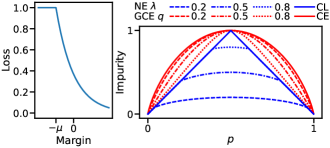
Figure 1: Left: NE loss as a function of the margin $y\widehat{y}$. Right: Blue lines are NE impurities with their $\lambda$ values provided in the legend. The special case with $\lambda=1$ is denoted by CL (conservative loss). Red lines are GCE impurities with their $q$ values provided in the legend. The special case with $q=0$ is denoted by CE (cross entropy). The impurities have been scaled for better comparison.

Theorem 8.

The NE loss’s partial empirical risk is given by

$$\widehat{R}(\widehat{y};{\cal{S}}) =\sum_{({\bm{x}},y)\in{\cal{S}}}\min\{1,\exp(-\widehat{y}y-\mu)\}/|{\cal{D}}|,$$

and the corresponding impurity (i.e., minimum partial empirical risk) is

$$\underset{\widehat{y}\in{\mathbb{R}}}{\min}\,\widehat{R}(\widehat{y};{\cal{S}}) ={W_{\cal{S}}}\min\left\{1-\|{\bm{p}}\|_{\infty},\ \lambda\sqrt{(1-\|{\bm{p}}\|_{2}^{2})/2}\right\},$$

with ${\bm{p}}=(p_{+},p_{-})^{\mathsf{T}}$, $p_{+}$ being the proportion of examples with $y=+1$ in ${\cal{S}}$ and $\lambda=2e^{-\mu}$.

Note that in the definition of the NE impurity above, $\widehat{y}$ ranges over ${\mathbb{R}}$ instead of over the 1-simplex. This is because we have chosen the prediction $\widehat{y}$ to be a positiveness score, instead of a two-dimensional vector representing a probability distribution, as done in the preliminaries section.

We provide a generalization of the NE impurity to the multiclass setting:

$$\underset{\widehat{y}\in{\mathbb{R}}}{\min}\,\widehat{R}(\widehat{y};{\cal{S}}) ={W_{\cal{S}}}\min\left\{1-\|{\bm{p}}\|_{\infty},\ \lambda\sqrt{\frac{1-\|{\bm{p}}\|_{2}^{2}}{K/(K-1)}}\right\}.$$

Clearly, this reduces to the binary NE impurity when $K=2$. The $K/(K-1)$ factor is chosen such that when $\lambda=1$, the two expressions under $\min$ have the same maximum value, a property that holds for the binary case in Theorem 8.

We visualize the NE impurity and compare it against the entropy, GCE, and misclassification impurities in Figure 1. The NE impurity interpolates between the misclassification impurity and the square root of the Gini impurity: for medium $p$ values, the NE impurity equals the square root of the Gini impurity (up to a multiplicative constant); while for small and large $p$ values, the NE impurity is the same as the misclassification impurity. In particular, we get the misclassification impurity for $\lambda=1$, and we get the square root of the Gini impurity as $\lambda\to 0$. In contrast, the GCE impurities (including entropy) upper bound the misclassification impurity.

The NE impurity supports an adaptive robustness mechanism: the robustness parameter $\lambda\in(0,1]$ controls the similarity between the NE impurity and the misclassification impurity, and it can be tuned to adapt to the noise rate, as done in our experiments. A larger $\lambda$ is associated with higher similarity with the misclassification impurity, thus encouraging more early stopping and higher robustness. An alternative effective way to control early stopping is setting the minimum number of samples in a leaf (Ghosh, Manwani, and Sastry 2017). Our method is distribution dependent and more flexible in the sense that it allows for leaf nodes with varying numbers of samples. We also note that the GCE impurity (Zhang and Sabuncu 2018) has a hyperparameter $q\in[0,1]$ controlling how it interpolates between the robust misclassification impurity and the non-robust entropy impurity. However, the early stopping property as in Theorem 5 only takes effect for $q\geq 1$. We see in experiments that varying $q$ between 0 and 1 does not seem to improve robustness to label noise for tree methods as a result.

Experiments

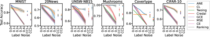
Figure 2: Mean test accuracy with 2x sd bands for DT on binary classification problems using different splitting criteria. Training labels corrupted using uniform noise $\eta\in\{0.0,0.1,0.2,0.3,0.4\}$ and class conditional noise CC1 $(0.1,0.3)$ and CC2 $(0.2,0.4)$.

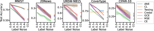
Figure 3: Mean test accuracy with 2x sd bands for DT on multiclass classification problems using different splitting criteria. Training labels corrupted using uniform noise $\eta\in\{0.0,0.1,0.2,0.3,0.4\}$ and class conditional (CC) noise.

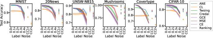
Figure 4: Mean test accuracy with 2x sd bands for RF on binary classification problems using different splitting criteria. Training labels corrupted using uniform noise $\eta\in\{0.0,0.1,0.2,0.3,0.4\}$ and class conditional noise CC1 $(0.1,0.3)$ and CC2 $(0.2,0.4)$.

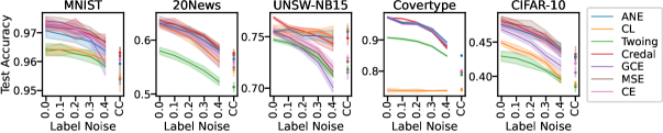
Figure 5: Mean test accuracy with 2x sd bands for RF on multiclass classification problems using different splitting criteria. Training labels corrupted using uniform noise $\eta\in\{0.0,0.1,0.2,0.3,0.4\}$ and class conditional (CC) noise.

In this section we empirically compare the NE loss with several other loss functions and tree growing methods. Selected baselines include NE loss, conservative losses (CLs), twoing split criteria (Breiman et al. 1984), Credal-C4.5 (Mantas and Abellan 2014), GCE loss (Zhang and Sabuncu 2018), ranking loss (Yang, Gao, and Li 2019), CE loss and MSE loss. Note that twoing, Gini and misclassification are shown to be robust with large number of samples at leaf in (Ghosh, Manwani, and Sastry 2017). We are interested in the predictive performance on clean test data of both decision trees and random forests trained using noisily labeled training data in various label noise settings. We also investigate the effect of tuning the hyperparameter $\lambda$ in the NE impurity.

Datasets

We consider some commonly used datasets from UCI including Covertype (Blackard 1998), 20News (Lang 1995), Mushrooms (Audubon Society Field Guide 1987), as well as the MNIST digits (LeCun et al. 1998), CIFAR-10 (Krizhevsky 2009) and UNSW-NB15 (Moustafa and Slay 2015). Datasets were selected due to diversity in number of samples, number of features, number of classes, type (image, tabular, text), and domain (computer vision, cyber security, cartography). We look at both multiclass ($K>2$) and binary ($K=2$) classification problems for each dataset. Mushrooms datasets and ranking loss excluded from multiclass classification experiments due to Mushrooms being a binary classification dataset, and ranking loss only defined for binary classification problems. Table 1 is a summary of the benchmark datasets.

Name	Train	Test	Feature	Class
MNIST Digits	60 000	10 000	784	10
CIFAR-10	50 000	10 000	3 072	10
20News	11 313	7 531	300	20
UNSW-NB15	175 341	82 332	39	10
Covertype	464 809	116 203	54	7
Mushrooms	6499	1625	112	2

Table 1: Benchmark datasets.

Binarized versions of labels are based on the processing in (Kiryo et al. 2017; Wilton et al. 2022). For 20News, GloVe pre-trained word embeddings (Pennington, Socher, and Manning 2014) were used (glove.840B.300d), then average pooling was applied over the word embeddings to generate the embedding for each document. The binarized classes are ‘alt., comp., misc., rec.’ versus ‘sci., soc., talk.’. For MNIST, the binarized classes are ‘0, 2, 4, 6, 8’ versus ‘1, 3, 5, 7, 9’ (even vs odd). For CIFAR-10, the binarized classes are ‘airplane, automobile, ship, truck’ versus ‘bird, cat, deer, dog, frog, horse’ (animal vs non-animal). For UNSW-NB15, we removed ID and the nominal features proto, service and state. The binarized labels are attack versus benign. For Covertype, the binarized classes are the second class versus others, as done in (Collobert, Bengio, and Bengio 2001), and the train-test split was performed using scikit-learn train_test_split with train_size 0.8 and random_state 0. For Mushrooms, we used the LIBSVM (Chang and Lin 2011) version, and the train-test split was performed identically as for Covertype.

Label Noise

We used both uniform noise and class conditional noise to corrupt the training labels, while testing labels had no noise applied. For uniform label noise, noise rates $\eta=0.0,\ 0.1,\ 0.2,\ 0.3$ and $0.4$ were used. For class conditional noise in binary classification two noise rates were used; $(0.1,0.3)$ and $(0.2,0.4)$. For multiclass classification, transition probabilities were constructed based on the similarity between classes using the Mahalanobis distance. See Algorithm 1 in Appendix J for details.

Hardware & Software

Experiments were performed using Python on a computer cluster with Intel Xeon E5 Family CPUs @ 2.20GHz and 192GB memory running CentOS.

Hyperparameters

Following common practice (Pedregosa et al. 2011), we set no restriction on maximum depth or number of leaf nodes, minimum one sample per leaf node, 100 trees in each RF, each using only $\sqrt{d}$ randomly chosen features, and predictions with RF made by majority average label distribution over all trees. The NE impurity hyperparameter $\lambda\in\{0,0.25,0.5,0.75,1\}$ was tuned by training on 80% of the noisy training set and validation on the other 20%. GCE $q=0.7$ as recommended for NNs (Zhang and Sabuncu 2018), Credal-C4.5 $s=1$ as recommended in (Mantas and Abellan 2014).

Classification Performance

We trained each model on 5 random noisy training sets to account for randomness in training labels and learning algorithms. We report the average test set accuracies and 2x standard deviation bands. Additional results can be found in Appendices K and L.

Effect of Loss Function on Robustness to Label Noise for Decision Trees

Decision tree results for binary and multiclass settings are summarized in Figures 2 and 3, respectively. Adaptive NE loss (ANE; NE with tuned $\lambda$) is almost always a top performer across all label noise settings, label configurations (binary, multiclass) and datasets. Conservative loss functions sometimes give poor performance in low noise settings, but usually give strong performance in high noise settings. CE, MSE, Ranking, GCE give similar performance. Twoing split criteria typically gives the worst performance. Credal-C4.5, across many noise settings and datasets, usually has performance somewhere between CE, MSE, Ranking, GCE and ANE.

Effect of Loss Function on Robustness to Label Noise for Random Forest

Random forest results for binary and multiclass settings are summarized in Figures 4 and 5, respectively. We first note that the differences in performance across loss functions are less significant than for decision trees in general, suggesting that an ensemble is more robust than a single tree. Note that RF still seems to boost performance of non-conservative loss functions, though this boost is less for conservative losses. Overall, ANE still shows strong performance.

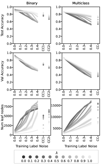
Figure 6: Performance of DT using NE loss with different values of $\lambda$ on MNIST digits, binary and multiclass classification, 20% of noisily labeled training data used for validation. Results reported as mean $\pm$ 2x sd over 5 replications.

Effect of NE Threshold on Predictive Performance and Tree Size

We investigated the effect of the robustness parameter $\lambda$ for the NE impurity by performing experiments on the MNIST digits dataset. The results in Figure 6 show that different $\lambda$ values often have best performance for different noise settings, without any single $\lambda$ value yielding the best performance in all cases. This together with the results in Figures 2 and 3 suggests that tuning $\lambda$ allows effective control on early stopping, and in turn, robustness to label noise. Additional discussion on early stopping in binary classification is provided in Appendix M.

Conclusions

We developed new insight and tools on robust loss functions for decision tree learning. We introduced the conservative loss as a general class of robust loss functions and provided several results showing their robustness in decision tree learning. In addition, we introduced the distribution loss as a general framework for building loss functions based CDFs, and instantiated it to introduce the robust NE loss. Our experiments demonstrated that our NE loss effectively alleviates the adverse effect of noise in various noise settings.

Appendix A Proof of Theorem 1

See 1

Proof.

(a) The MSE is

$$\widehat{R}_{\mathrm{MSE}}(\widehat{{\bm{y}}};{\cal{S}}) =\sum_{({\bm{x}},{\bm{y}})\in{\cal{S}}}\|\widehat{{\bm{y}}}-{\bm{y}}\|_{2}^{2}/|{\cal{D}}|.$$

Setting the gradient to 0,

$$\nabla_{\widehat{{\bm{y}}}}\widehat{R}_{\mathrm{MSE}}(\widehat{{\bm{y}}};{\cal{S}})=\sum_{({\bm{x}},{\bm{y}})\in{\cal{S}}}\frac{2(\widehat{{\bm{y}}}-{\bm{y}})}{|{\cal{D}}|}=2W_{{\cal{S}}}(\widehat{{\bm{y}}}-{\bm{p}})=0.$$

Solving the equation gives

$$\widehat{{\bm{y}}}^{*} ={\bm{p}}.$$

Hence, knowing that ${\bm{p}}$ and each of $\{{\bm{y}}\}$ are probability vectors, the minimum partial empirical risk is

$$\widehat{R}_{\mathrm{MSE}}^{*}({\cal{S}}) =\sum_{({\bm{x}},{\bm{y}})\in{\cal{S}}}\|{\bm{p}}-{\bm{y}}\|_{2}^{2}/|{\cal{D}}|,$$

$$=\frac{1}{|{\cal{D}}|}\sum_{({\bm{x}},{\bm{y}})\in{\cal{S}}}\left[\|{\bm{p}}\|_{2}^{2}+1-2{\bm{p}}^{\mathsf{T}}{\bm{y}}\right],$$

$$=W_{{\cal{S}}}\|{\bm{p}}\|_{2}^{2}+W_{{\cal{S}}}-2W_{{\cal{S}}}{\bm{p}}^{\mathsf{T}}{\bm{p}},$$

$$=W_{{\cal{S}}}(1-\|{\bm{p}}\|_{2}^{2}).$$

(b) For the CE loss, the partial empirical risk can be simplified by grouping together examples with common labels

$$\widehat{R}_{\mathrm{CE}}(\widehat{{\bm{y}}};{\cal{S}}) =-\frac{1}{|{\cal{D}}|}\sum_{({\bm{x}},{\bm{y}})\in{\cal{S}}}{\bm{y}}^{\mathsf{T}}\log\widehat{{\bm{y}}},$$

$$=-W_{{\cal{S}}}\sum_{j=1}^{K}p_{j}\log\widehat{y}_{j}.$$

Use Lagrange multiplier to ensure solution sums to one

$$\mathcal{L}(\widehat{{\bm{y}}},\lambda) :=-W_{{\cal{S}}}\sum_{j=1}^{K}p_{j}\log\widehat{y}_{j}+\lambda\left(\sum_{j=1}^{K}\widehat{y}_{j}-1\right).$$

The $k$-th component of the optimal constant probability vector prediction satisfies the equation

$$\frac{\partial\mathcal{L}}{\partial\widehat{y}_{k}}=-W_{{\cal{S}}}p_{k}/\widehat{y}_{k}+\lambda=0.$$

Solving this equation gives $\widehat{y}_{k}^{*}={W_{\cal{S}}}p_{k}/\lambda$. Applying the constraint to solve for $\lambda$ gives

$$1 =\sum_{j=1}^{K}\widehat{y}_{j}^{*}=\sum_{j=1}^{K}{W_{\cal{S}}}p_{k}/\lambda={W_{\cal{S}}}/\lambda,$$

$$\lambda ={W_{\cal{S}}}.$$

Plugging the optimal $\lambda$ into the expression for $\widehat{y}_{j}^{*}$, we obtain

$$\widehat{{\bm{y}}}^{*} ={\bm{p}},$$

$$\widehat{R}_{\mathrm{CE}}^{*}({\cal{S}}) ={W_{\cal{S}}}(-{\bm{p}}^{\mathsf{T}}\log{\bm{p}}).$$

(c) The form of the partial empirical risk can be simplified based on the prediction $\widehat{{\bm{y}}}$

$$\widehat{R}_{01}(\widehat{{\bm{y}}};{\cal{S}}) =\frac{1}{|{\cal{D}}|}\sum_{({\bm{x}},{\bm{y}})\in{\cal{S}}}\mathds{1}(\widehat{{\bm{y}}}\neq{\bm{y}}),$$

$$={W_{\cal{S}}}\sum_{j=1}^{K}p_{j}\mathds{1}(\widehat{{\bm{y}}}\neq{\bm{e}}_{j}),$$

$$={W_{\cal{S}}}\begin{cases}1,&\widehat{{\bm{y}}}\notin\{{\bm{e}}_{j}\}_{j=1}^{K},\\ 1-p_{j},&\widehat{{\bm{y}}}={\bm{e}}_{j}.\end{cases}$$

The prediction $\widehat{{\bm{y}}}^{*}$ that minimizes the partial empirical risk is thus

$$\widehat{{\bm{y}}}^{*} =\bm{e}_{\mathrm{argmax}({\bm{p}})},$$

with optimal risk

$$\widehat{R}_{01}^{*}({\cal{S}}) ={W_{\cal{S}}}(1-\|{\bm{p}}\|_{\infty}).$$

(d) For $q=0$, the GCE loss is identical to CE loss (Zhang and Sabuncu 2018), and hence both loss functions lead to the same impurity.

Fix $q\in(0,1)$. The partial empirical GCE risk with constant prediction $\widehat{{\bm{y}}}$ is

$$\widehat{R}_{\mathrm{GCE}}(\widehat{{\bm{y}}};{\cal{S}}) =\frac{1}{|{\cal{D}}|}\sum_{({\bm{x}},{\bm{y}})\in{\cal{S}}}\frac{1-({\bm{y}}^{\mathsf{T}}\widehat{{\bm{y}}})^{q}}{q},$$

$$={W_{\cal{S}}}\sum_{j=1}^{K}p_{j}\frac{1-\widehat{y}_{j}^{q}}{q},$$

$$={W_{\cal{S}}}(1-\sum_{j=1}^{K}p_{j}\widehat{y}_{j}^{q})/q.$$

By Hölder’s inequality we have

$$\sum_{j=1}^{K}p_{j}\widehat{y}_{j}^{q} \leq\|{\bm{p}}\|_{1/(1-q)}\left(\sum_{j=1}^{K}(\widehat{y}_{j}^{q})^{1/q}\right)^{q},$$

$$=\|{\bm{p}}\|_{1/(1-q)}\left(\sum_{j=1}^{K}\widehat{y}_{j}\right)^{q}.$$

We get equality in Hölder’s inequality if and only if $\widehat{y}_{j}^{q}\propto p_{j}^{1/(1-q)-1},\,\forall j=1,\ldots,K$. Therefore, we can choose $\widehat{{\bm{y}}}^{*}$ to be the probability vector with elements $\widehat{y}_{j}^{*}=p_{j}^{1/(1-q)}/\sum_{k=1}^{K}p_{k}^{1/(1-q)},\,\forall j=1,\ldots,K$. Hence, the minimum partial empirical risk becomes

$$\widehat{R}_{\mathrm{GCE}}^{*}({\cal{S}}) ={W_{\cal{S}}}(1-\|{\bm{p}}\|_{1/(1-q)})/q.$$

Now let $q>1$. Similarly as for the case $q\in(0,1)$ we can simplify by grouping together examples from each class

$$\widehat{R}_{\mathrm{GCE}}(\widehat{{\bm{y}}};{\cal{S}}) ={W_{\cal{S}}}(1-\sum_{j=1}^{k}p_{j}\widehat{y}_{j}^{q})/q.$$

Using $\widehat{{\bm{y}}}\in\Delta$ and $q>1$, we have $\widehat{y}_{j}^{q}\leq\widehat{y}_{j}\,\forall j=1,\ldots,K$ and $\sum_{j=1}^{K}p_{j}\widehat{y}_{j}\leq\max_{j}p_{j}=\|{\bm{p}}\|_{\infty}$. Combining these facts results in

$${W_{\cal{S}}}(1-\sum_{j=1}^{k}p_{j}\widehat{y}_{j}^{q})/q \geq{W_{\cal{S}}}(1-\sum_{j=1}^{k}p_{j}\widehat{y}_{j})/q,$$

$$\geq{W_{\cal{S}}}(1-\|{\bm{p}}\|_{\infty})/q.$$

We have equality in the above for $\widehat{{\bm{y}}}^{*}={\bm{e}}_{\mathrm{argmax}({\bm{p}})}$, giving optimal objective value

$$\widehat{R}_{\mathrm{GCE}}^{*}({\cal{S}}) ={W_{\cal{S}}}(1-\|{\bm{p}}\|_{\infty})/q.$$

(e) Using the fact that $\widehat{{\bm{y}}}\in\Delta$ and ${\bm{y}}\in\{{\bm{e}}_{j}\}_{j=1}^{K}$ for each ${\bm{y}}\in{\cal{S}}$, the partial empirical risk can be simplified as

$$\widehat{R}_{\mathrm{MAE}}(\widehat{{\bm{y}}};{\cal{S}}) =\frac{1}{|{\cal{D}}|}\sum_{({\bm{x}},{\bm{y}})\in{\cal{S}}}\|\widehat{{\bm{y}}}-{\bm{y}}\|_{1},$$

$$=\frac{1}{|{\cal{D}}|}\sum_{({\bm{x}},{\bm{y}})\in{\cal{S}}}2-2\widehat{{\bm{y}}}^{\mathsf{T}}{\bm{y}},$$

$$=2{W_{\cal{S}}}(1-\widehat{{\bm{y}}}^{\mathsf{T}}{\bm{p}}).$$

Since $\widehat{{\bm{y}}}^{\mathsf{T}}{\bm{p}}=\sum_{j=1}^{K}\widehat{y}_{j}p_{j}$ is a convex combination of the values $\{p_{j}\}$ with weights $\{\widehat{y}_{j}\}$, we have $\widehat{{\bm{y}}}^{\mathsf{T}}{\bm{p}}\leq\max_{j}p_{j}=\|{\bm{p}}\|_{\infty}$, with equality achieved for

$$\widehat{{\bm{y}}}^{*} ={\bm{e}}_{\mathrm{argmax}({\bm{p}})}.$$

Plugging the optimal prediction into the objective gives the result

$$\widehat{R}_{\mathrm{MAE}}^{*}({\cal{S}}) =2{W_{\cal{S}}}(1-\|{\bm{p}}\|_{\infty}).\qed$$

Appendix B Proof of Theorem 2

The proof of Theorem 2 relies on Lemma 9.

Lemma 9.

Let $(p_{1},\ldots,p_{K})\in\Delta$ be a probability vector and $\{\ell_{j}\}_{j=1}^{K}\subset{\mathbb{R}}$ be a set of constants. If

1. $p_{1}\leq\cdots\leq p_{K}$,

2. $\sum_{j=1}^{K}\ell_{j}\geq C(K-1)$ and

3. $0\leq\ell_{j}\leq C,\,\forall j=1,\ldots,K$,

then

$$\sum_{j=1}^{K}p_{j}l_{j} \geq C(1-p_{K}).$$ (3)

Proof.

Assume each of $(a)$, $(b)$ and $(c)$ are true. Starting with the right hand side of (3), we can write

$$C(1-p_{K})=\sum_{j\neq K}p_{j}C$$

$$= \sum_{j\neq K}p_{j}(\ell_{j}+(C-\ell_{j}))+p_{K}(\ell_{K}+\sum_{j\neq K}\ell_{j}-\sum_{j=1}^{K}\ell_{j}),$$

$$\leq \sum_{j\neq K}p_{j}(\ell_{j}+(C-\ell_{j}))$$

$$\quad+p_{K}(\ell_{K}+\sum_{j\neq K}\ell_{j}-C(K-1)),$$

$$= \sum_{j\neq K}p_{j}(\ell_{j}+(C-\ell_{j}))+p_{K}(\ell_{K}-\sum_{j\neq K}(C-\ell_{j})),$$

$$= \sum_{j\neq K}p_{j}\ell_{j}+\sum_{j\neq K}p_{j}(C-\ell_{j})$$

$$\quad+p_{K}\ell_{K}-\sum_{j\neq K}p_{K}(C-\ell_{j}),$$

$$= \sum_{j=1}^{K}p_{j}\ell_{j}+\sum_{j\neq K}(p_{j}-p_{K})(C-\ell_{j}),$$

$$\leq \sum_{j=1}^{K}p_{j}\ell_{j}.\qed$$

See 2

Proof.

If $\ell$ is conservative, then we can use Lemma 9 with the sorted version of ${\bm{p}}$ and constants $\{\ell(\widehat{{\bm{y}}},{\bm{e}}_{j})\}_{j=1}^{K}$ to give

$$\widehat{R}(\widehat{{\bm{y}}};{\cal{S}})={W_{\cal{S}}}\sum_{j=1}^{K}p_{j}\ell(\widehat{{\bm{y}}},{\bm{e}}_{j})\geq C{W_{\cal{S}}}(1-\|{\bm{p}}\|_{\infty}).$$ (4)

The lower bound in Eq. 4 can be achieved by choosing $k=\mathrm{argmax}({\bm{p}}),\ \widehat{{\bm{y}}}={\bm{e}}_{k}$. Indeed, by $(a)$, $(b)$ and $(c)$ from the definition of the conservative loss, we have $\ell({\bm{e}}_{k},{\bm{e}}_{k})=0$ and $\ell({\bm{e}}_{k},{\bm{e}}_{j})=C,\ j\neq k$, giving

$$\widehat{R}^{*}({\cal{S}}) =\widehat{R}({\bm{e}}_{k};{\cal{S}}),$$

$$={W_{\cal{S}}}\sum_{j=1}^{K}p_{j}\ell({\bm{e}}_{k},{\bm{e}}_{j}),$$

$$=C{W_{\cal{S}}}\sum_{j\neq k}p_{j},$$

$$=C{W_{\cal{S}}}(1-\|{\bm{p}}\|_{\infty}).$$

Now we show that Eq. 2 implies (a) in 1. Assume $(a)$ is false, then there exists $\widehat{y}$ such that $\sum_{j=1}^{K}\ell(\widehat{{\bm{y}}},{\bm{e}}_{j})<C(K-1)$. Consider an ${\cal{S}}$ with its corresponding ${\bm{p}}$ being the uniform distribution, then,

$$\quad\widehat{R}^{*}({\cal{S}})$$

$$\leq\widehat{R}(\widehat{{\bm{y}}};{\cal{S}})=\frac{1}{|{\cal{D}}|}\sum_{({\bm{x}},{\bm{y}})\in{\cal{S}}}\ell(\widehat{{\bm{y}}},{\bm{y}})$$

$$={W_{\cal{S}}}\sum_{j=1}^{K}p_{j}\ell(\widehat{{\bm{y}}},{\bm{e}}_{j})={W_{\cal{S}}}\frac{1}{K}\sum_{j=1}^{K}\ell(\widehat{{\bm{y}}},{\bm{e}}_{j})$$

$$<{W_{\cal{S}}}\frac{1}{K}C(K-1)=C{W_{\cal{S}}}(1-1/K)$$

$$=C{W_{\cal{S}}}(1-\|{\bm{p}}\|_{\infty}).$$

That is, $\widehat{R}^{*}({\cal{S}})<C{W_{\cal{S}}}(1-\|{\bm{p}}\|_{\infty})$, a contradiction. Therefore, Eq. 2 implies (a). ∎

Appendix C Proof of Corollary 2.1

See 2.1

Proof.

To show this, we need to show that the conditions of Theorem 2 are satisfied for each loss function. Fix $\widehat{{\bm{y}}}\in\Delta$ and $k\in\{1,\ldots,K\}$. We first check condition $(a)$:

$$\ell( \widehat{{\bm{y}}},{\bm{e}}_{k})=$$

$$\begin{cases}\|\widehat{{\bm{y}}}-{\bm{e}}_{k}\|_{1}=2-2\widehat{y}_{k}\leq 2&\mathrm{MAE},\\ \mathds{1}(\widehat{{\bm{y}}}\neq{\bm{e}}_{k})\leq 1&01,\\ \frac{1}{q}(1-({\bm{e}}_{k}^{\mathsf{T}}\widehat{{\bm{y}}})^{q})=\frac{1}{q}(1-\widehat{y}_{k}^{q})\leq\frac{1}{q}&\mathrm{GCE},\\ \|\widehat{{\bm{y}}}-{\bm{e}}_{k}\|_{\infty}=\max(1-\widehat{y}_{k},\,\underset{j\neq k}{\max}\,\widehat{y}_{j})\leq 1&\mathrm{INF}.\end{cases}$$

Then for condition $(b)$:

$$\sum_{j=1}^{K} \ell(\widehat{{\bm{y}}},{\bm{e}}_{j})=$$

$$\begin{cases}\sum_{j=1}^{K}(2-2\widehat{y}_{j})=2(K-1)&\mathrm{MAE},\\ \sum_{j=1}^{K}\mathds{1}(\widehat{{\bm{y}}}\neq{\bm{e}}_{j})\geq K-1&01,\\ \sum_{j=1}^{K}\frac{1}{q}(1-\widehat{y}_{j}^{q})\geq\frac{1}{q}(K-1)&\mathrm{GCE},\\ \sum_{j=1}^{K}\max(1-\widehat{y}_{j},\,\underset{i\neq j}{\max}\,\widehat{y}_{i})\geq K-1&\mathrm{INF}.\end{cases}$$

Finally condition $(c)$. Note that for $\widehat{{\bm{y}}}={\bm{e}}_{k}$, we have $\widehat{y}_{k}=1$, so,

$$\ell({\bm{e}}_{k},{\bm{e}}_{k})=\begin{cases}(2-2)=0&\mathrm{MAE},\\ \mathds{1}(1=0)=0&01,\\ \frac{1}{q}(1-1^{q})=0&\mathrm{GCE},\\ \max(1-1,\,0)=0&\mathrm{INF}.\end{cases}\qed$$

Appendix D Proof of Theorem 3

See 3

Proof.

If $\ell$ is conservative, then the if-part of the proof of Theorem 2 shows that the minimum partial impurity is achieved by $\widehat{{\bm{y}}}={\bm{e}}_{\mathrm{argmax}({\bm{p}})}$, with

$$\widehat{R}({\bm{e}}_{\mathrm{argmax}({\bm{p}})};{\cal{S}})=C(1-\|{\bm{p}}\|_{\infty}).$$

As seen in the proof of Theorem 1 $(a)$, the partial empirical risk with MSE loss takes on its minimum value of the Gini impurity for $\widehat{{\bm{y}}}={\bm{p}}$. Similarly for the CE loss, as seen in the proof of Theorem 1 $(b)$, the partial empirical risk takes on its minimum value of the entropy impurity for $\widehat{{\bm{y}}}={\bm{p}}$. ∎

Appendix E Proof of Theorem 4

See 4

Proof.

The probability that the majority class in $\widetilde{{\cal{S}}}$ remains the same as in ${\cal{S}}$ is

$$\;{\mathbb{P}}(\widetilde{p}_{k^{*}}\geq\widetilde{p}_{k}\text{for all $k\neq k^{*}$}\,|\,{\cal{S}})$$

$$= \;1-{\mathbb{P}}(\widetilde{p}_{k^{*}}<\widetilde{p}_{k}\text{for at least one $k\neq k^{*}$}\,|\,{\cal{S}}).$$

By Boole’s inequality (i.e., the union bound),

$$\;1-{\mathbb{P}}(\widetilde{p}_{k^{*}}<\widetilde{p}_{k}\text{for at least one $k\neq k^{*}$}\,|\,{\cal{S}})$$

$$\geq \;1-\sum_{k\neq k^{*}}{\mathbb{P}}\left(\widetilde{p}_{k^{*}}<\widetilde{p}_{k}\,|\,{\cal{S}}\right)$$

$$\geq \;1-\sum_{k\neq k^{*}}{\mathbb{P}}\left(\widetilde{p}_{k}-\widetilde{p}_{k^{*}}\geq 0\,|\,{\cal{S}}\right).$$ (5)

We shall use Hoeffding’s inequality to bound each ${\mathbb{P}}\left(\widetilde{p}_{k}-\widetilde{p}_{k^{*}}\geq 0\,|\,{\cal{S}}\right)$ for each $k\neq k^{*}$, because $\widetilde{p}_{k}-\widetilde{p}_{k^{*}}$ is the average of the independent random variables $\{\widetilde{y}_{ik^{*}}-\widetilde{y}_{ik}\}_{i=1}^{n}$ which take values in $[-1,1]$.

Since the noise is uniform with rate $\eta$, we have

$$\widetilde{p}_{k}^{\eta} ={\mathbb{E}}[\widetilde{p}_{k}]=(1-\eta)p_{k}+\frac{\eta}{K-1}\sum_{j\neq k}p_{j}$$

$$=\left(1-\frac{K\eta}{K-1}\right)p_{j}+\frac{\eta}{K-1}.$$

In addition, since $\eta<(K-1)/K$, we have for any $k\neq k^{*}$,

$$t_{k}:=\widetilde{p}_{k^{*}}^{\eta}-\widetilde{p}_{k}^{\eta}=\left(1-\frac{K\eta}{K-1}\right)(p_{k^{*}}-p_{k})>0.$$

Applying Hoeffding’s inequality, we have

$$\;{\mathbb{P}}\left(\widetilde{p}_{k}-\widetilde{p}_{k^{*}}\geq 0\,|\,{\cal{S}}\right)$$ (6)

$$= \;{\mathbb{P}}\left(\widetilde{p}_{k}-\widetilde{p}_{k^{*}}\geq t_{k}+(\widetilde{p}_{k}^{\eta}-\widetilde{p}_{k^{*}}^{\eta})\,|\,{\cal{S}}\right)$$

$$\leq \;\exp\left(-nt_{k}^{2}/2\right)$$

$$\leq \;\exp\left(-n\gamma^{2}/2\right),$$ (7)

where $\gamma=\underset{k\neq k^{*}}{\min}\,(p_{k^{*}}-p_{k})$ is the margin.

Plugging the bound in Eq. 7 into Eq. 5, we have

$${\mathbb{P}}(\widetilde{p}_{k^{*}}\geq\widetilde{p}_{k}\text{ for all $k\neq k^{*}$}\,|\,{\cal{S}}) \geq 1-(K-1)e^{-n\gamma^{2}/2}.\qed$$

Appendix F Proof of Theorem 5

The proof of Theorem 5 relies on the result in Lemma 10.

Lemma 10.

Let ${\bm{x}}=(x_{1},\ldots,x_{d})^{\mathsf{T}},{\bm{y}}=(y_{1},\ldots,y_{d})^{\mathsf{T}}\in{\mathbb{R}}_{\geq 0}^{d}$ be $d$-dimensional vectors of nonnegative real numbers and ${\mathscr{M}}_{{\bm{z}}}=\{j:z_{j}=\|{\bm{z}}\|_{\infty}\}$ be the set of indices corresponding to maximal elements of ${\bm{z}}$, for any ${\bm{z}}\in{\mathbb{R}}_{\geq 0}^{d}$. Then,

$$\|{\bm{x}}+{\bm{y}}\|_{\infty}=\|{\bm{x}}\|_{\infty}+\|{\bm{y}}\|_{\infty}$$

if and only if

$${\mathscr{M}}_{{\bm{x}}+{\bm{y}}}={\mathscr{M}}_{{\bm{x}}}\cap{\mathscr{M}}_{{\bm{y}}}.$$

Proof.

(if) Assume ${\mathscr{M}}_{{\bm{x}}+{\bm{y}}}={\mathscr{M}}_{{\bm{x}}}\cap{\mathscr{M}}_{{\bm{y}}}$, and let $i\in{\mathscr{M}}_{{\bm{x}}+{\bm{y}}}$. Then, $i\in{\mathscr{M}}_{{\bm{x}}}$, $i\in{\mathscr{M}}_{{\bm{y}}}$, and

$$\|{\bm{x}}+{\bm{y}}\|_{\infty} =x_{i}+y_{i},$$

$$\|{\bm{x}}\|_{\infty} =x_{i},$$

$$\|{\bm{y}}\|_{\infty} =y_{i}.$$

Thus, $\|{\bm{x}}+{\bm{y}}\|_{\infty}=\|{\bm{x}}\|_{\infty}+\|{\bm{y}}\|_{\infty}$.

(only if) Assume $\|{\bm{x}}+{\bm{y}}\|_{\infty}=\|{\bm{x}}\|_{\infty}+\|{\bm{y}}\|_{\infty}$, and let $i\in\mathscr{M}_{{\bm{x}}}$, $j\in\mathscr{M}_{{\bm{y}}}$, $k\in\mathscr{M}_{{\bm{x}}+{\bm{y}}}$. Then, by assumption, we have

$$x_{k}+y_{k}=x_{i}+y_{j},$$

if and only if

$$x_{k}-x_{i}=y_{j}-y_{k}.$$ (8)

The LHS of Eq. 8 is at most zero, and the RHS of Eq. 8 is at least zero. We achieve equality if and only if both sides are zero, which happens when $k\in{\mathscr{M}}_{{\bm{x}}}\cap{\mathscr{M}}_{{\bm{y}}}$. Since $k$ is an arbitrary element of ${\mathscr{M}}_{{\bm{x}}+{\bm{y}}}$, we must have ${\mathscr{M}}_{{\bm{x}}+{\bm{y}}}\subseteq{\mathscr{M}}_{{\bm{x}}}\cap{\mathscr{M}}_{{\bm{y}}}$. If we let $l\in{\mathscr{M}}_{{\bm{x}}}\cap{\mathscr{M}}_{{\bm{y}}}$, then by analogous reasoning we must have $l\in{\mathscr{M}}_{{\bm{x}}+{\bm{y}}}$. Therefore,

$${\mathscr{M}}_{{\bm{x}}+{\bm{y}}}={\mathscr{M}}_{{\bm{x}}}\cap{\mathscr{M}}_{{\bm{y}}}.\qed$$

See 5

Proof.

(a) Consider a conservative loss $\ell$ with associated positive constant $C$, a node containing a set of examples ${\cal{S}}$, and an arbitrary split $(f,t)$. Let ${\bm{p}}_{{\cal{S}}}$ be the vector of proportions of data in ${\cal{S}}$ from each class, and $\bm{n}_{{\cal{S}}}$ be the vector containing the number of examples in ${\cal{S}}$ from each class. Then, we have ${\rm RR}(f,t;{\cal{S}})\leq 0$ if and only if

$$C{W_{\cal{S}}}(1-\|{\bm{p}}_{{\cal{S}}}\|_{\infty})\leq\ CW_{{\cal{S}}_{f\leq t}}(1-\|{\bm{p}}_{{\cal{S}}_{f\leq t}}\|_{\infty})$$

$$+CW_{{\cal{S}}_{f>t}}(1-\|{\bm{p}}_{{\cal{S}}_{f>t}}\|_{\infty}),$$

which is equivalent to

$$|{\cal{S}}|(1-\|{\bm{p}}_{{\cal{S}}}\|_{\infty})\leq \ |{\cal{S}}_{f\leq t}|(1-\|{\bm{p}}_{{\cal{S}}_{f\leq t}}\|_{\infty})$$

$$+|{\cal{S}}_{f>t}|(1-\|{\bm{p}}_{{\cal{S}}_{f>t}}\|_{\infty}).$$

Using $|{\cal{S}}_{f\leq t}|+|{\cal{S}}_{f>t}|=|{\cal{S}}|$ gives:

$$\|\bm{n}_{{\cal{S}}}\|_{\infty} \geq\|\bm{n}_{{\cal{S}}_{f\leq t}}\|_{\infty}+\|\bm{n}_{{\cal{S}}_{f>t}}\|_{\infty}.$$ (9)

However, it is always true that $\|\bm{n}_{{\cal{S}}}\|_{\infty}\leq\|\bm{n}_{{\cal{S}}_{f\leq t}}\|_{\infty}+\|\bm{n}_{{\cal{S}}_{f>t}}\|_{\infty}$ by the triangle inequality, hence we stop splitting when equality in (9) is achieved. By Lemma 10, this happens only when the majority classes at the parent node are also the majority classes at both child nodes for the split $(f,t)$.

(b) For the MSE, it was shown in (Breiman et al. 1984) that ${\rm RR}_{\mathrm{MSE}}(f,t;{\cal{S}})\leq 0$ only when ${\bm{p}}_{{\cal{S}}}={\bm{p}}_{{\cal{S}}_{f\leq t}}={\bm{p}}_{{\cal{S}}_{f>t}}$ since $\widehat{R}_{\mathrm{MSE}}^{*}$, when viewed as a function of ${\bm{p}}_{{\cal{S}}}$, is strictly concave.

Since $\widehat{R}^{*}$ is also strictly concave for both the CE and GCE $(q\in(0,1))$ loss when viewed as a function of ${\bm{p}}_{{\cal{S}}}$, the same result holds as for MSE. ∎

Appendix G Proof of Lemma 6

See 6

Proof.

The CDF of the ${\mathsf{Ber}}(0)$ distribution is

$$F(x)=\mathds{1}(x\geq 0)=(1-\mathrm{sign}(-x))/2.$$

The loss function is thus

$$\ell(z)=F(-z)=(1-\mathrm{sign}(z))/2,$$

which is the 01 loss.

The CDF of the Logistic distribution with location 0 and scale 1 is

$$F(x)=1/(1+\exp(-x)).$$

The corresponding loss function is

$$\ell(z)=F(-z)=1/(1+\exp(x)),$$

which is the sigmoid loss.

The CDF of the $\mathsf{U}(-1,1)$ distribution is

$$F(x) =\frac{x+1}{2}\mathds{1}(x\in[-1,1])+\mathds{1}(x>1)$$

$$=\max\{0,\min\{1,(1+z)/2\}\}.$$

The corresponding loss function is

$$\ell(z)=F(-z)=\max\{0,\min\{1,(1-z)/2\}\},$$

which is the ramp loss. ∎

Appendix H Proof of Lemma 7

See 7

Proof.

Let $X$ be a random variable having an exponential distribution with scale $\beta$. Then the CDF of $X$ is $F(x)=\max\{0,1-\exp(-x/\beta)\}$. The CDF of its shifted negative $Z=\mu-X$ is

$$F(z) =1-\max\{0,1-\exp(-(\mu-z)/\beta)\}$$

$$=\min\{1,\exp((z-\mu)/\beta)\}.$$ (10)

Using $\beta=1$ and plugging $z\leftarrow-y\hat{y}$ into Eq. 10 gives the result. ∎

Appendix I Proof of Theorem 8

See 8

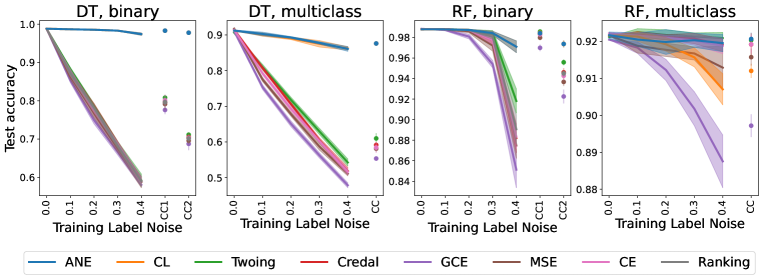
Figure 7: Mean test accuracy with 2x standard deviation bands for decision tree and random forest with different splitting criteria. Training labels corrupted using uniform noise $\eta\in\{0.0,0.1,0.2,0.3,0.4\}$ and class conditional noise CC1, CC2 for binary classification and CC for multiclass classification.

Proof.

Simplifying the partial empirical risk by grouping together the positive and negative samples gives

$$\;\widehat{R}(\widehat{y};{\cal{S}})$$

$$= \;\sum_{({\bm{x}},y)\in{\cal{S}}}\min\{1,e^{-\widehat{y}y-\mu)}\}/|{\cal{D}}|$$

$$= \;{W_{\cal{S}}}\left(p_{-}\min\{1,e^{\widehat{y}-\mu}\}+p_{+}\min\{1,e^{-\widehat{y}-\mu}\}\right)$$

$$= \;\begin{cases}{W_{\cal{S}}}\left(p_{-}e^{\widehat{y}-\mu}+p_{+}\right),&\widehat{y}\leq-\mu,\\ {W_{\cal{S}}}\left(p_{-}e^{\widehat{y}-\mu}+p_{+}e^{-\widehat{y}-\mu}\right),&-\mu<\widehat{y}<\mu,\\ {W_{\cal{S}}}\left(p_{-}+p_{+}e^{-\widehat{y}-\mu}\right),&\widehat{y}\geq\mu.\end{cases}$$

We consider the above three cases separately.

• When $\widehat{y}\leq-\mu$, the infimum is $p_{+}$, achieved when $\widehat{y}=-\infty$.

• When $-\mu<\widehat{y}<\mu$, using the fact that $a+b\geq 2\sqrt{ab}$ for $a,b\geq 0$ with equality when $a=b$, we have

  $$p_{-}e^{\widehat{y}-\mu}+p_{+}e^{-\widehat{y}-\mu}\geq 2e^{-\mu}\sqrt{p_{-}p_{+}}.$$

  The infimum is obtained when $p_{-}e^{\widehat{y}-\mu}=p_{+}e^{-\widehat{y}-\mu}$.

• When $\widehat{y}\geq\mu$, the infimum is $p_{-}$, achieved when $\widehat{y}=+\infty$.

Therefore we can write

$$\widehat{R}^{*}({\cal{S}}) =\min\{p,1-p,2e^{-\mu}\sqrt{p(1-p)}\}$$

$$=\min\left\{1-\|{\bm{p}}\|_{\infty},\,\lambda\sqrt{(1-\|{\bm{p}}\|_{2}^{2})/2}\right\}.\qed$$

Appendix J Class Conditional Noise

The method used for corrupting labels with class conditional noise in multiclass classification problems is based on the Mahalanobis distance between classes. Let $\overline{{\bm{x}}}_{1}$ and $\overline{{\bm{x}}}_{2}$ be the sample mean vectors of examples in classes 1 and 2, respectively, and $\mathbf{S}$ be the estimated common covariance matrix computed using feature vectors for the two classes. Then, the Mahalanobis distance between class 1 and 2 is defined to be $\sqrt{(\overline{{\bm{x}}}_{1}-\overline{{\bm{x}}}_{2})^{\mathsf{T}}\mathbf{S}^{-1}(\overline{{\bm{x}}}_{1}-\overline{{\bm{x}}}_{2})}$.

Transition probabilities on the off diagonals of $(\eta_{ij})_{i,j=1}^{K}$ are larger for pairs of classes with high similarity (in terms of Mahalanobis distance), and transition probabilities on the diagonals are smaller for those classes whose total similarity to every other class is high. Pseudocode for the algorithm used to generate noise rates is given in Algorithm 1.

Algorithm 1 Class Conditional Noise

Input: Data $\{({\bm{x}}_{i},{\bm{y}}_{i})\}_{i=1}^{n}$.
Output: Transition probabilities $(\eta_{ij})_{i,j=1}^{K}$.

1:  Compute $s_{ij}$, the inverse Mahalanobis distance between class $i$ and class $j$, for all $i\neq j$.

2:  Compute $s_{ii}=\sum_{j\neq i}1/s_{ij}$ for each class $i$.

3:  Scale $s_{ii}$ to range from 0.5 to 0.9.

4:  For all $i,j$, set $\eta_{ij}$ to $\begin{cases}s_{ij}/(1-s_{ii}),&i\neq j,\\ s_{ii},&i=j.\end{cases}$.

5:  Return: Transition probabilities $(\eta_{ij})_{i,j=1}^{K}$

Appendix K Pre-trained Image Embeddings CIFAR-10

We performed additional experiments on CIFAR-10 using pre-trained image embeddings from VGG11. The input to the last classifier module in the network was taken to be the new feature vectors. Other processing steps are the same as in the other experiments.

From Figure 7 we see that predictive performance of all tree methods generally improve compared to using the raw pixel values as in Figures 2, 3, 4 and 5. ANE still shows strong performance, generally performing the best across all noise settings, and particularly with large amounts of noise.

Appendix L Detailed Experiment Results

Tables 2, 3, 4 and 5 present the average accuracies and 2 standard deviations used in Figures 2, 3, 4 and 5. Best performers (and equivalent) are highlighted for each dataset and noise setting.

		Uniform Noise					Class Conditional
Dataset	Split Crit.	$0.0$	$0.1$	$0.2$	$0.3$	$0.4$	$(0.1,0.3)$	$(0.2,0.4)$
MNIST	ANE	$\mathbf{94.00\pm 0.48}$	$\mathbf{89.92\pm 0.84}$	$\mathbf{87.89\pm 1.37}$	$\mathbf{84.13\pm 3.35}$	$\mathbf{82.03\pm 1.39}$	$\mathbf{82.20\pm 1.35}$	$\mathbf{77.80\pm 1.65}$
	CL	$88.14\pm 0.08$	$86.94\pm 2.88$	$\mathbf{86.07\pm 3.04}$	$\mathbf{84.76\pm 2.42}$	$\mathbf{81.56\pm 2.06}$	$\mathbf{82.41\pm 1.19}$	$\mathbf{79.03\pm 2.49}$
	Twoing	$90.34\pm 0.48$	$82.99\pm 1.00$	$75.31\pm 1.52$	$66.66\pm 0.92$	$57.98\pm 1.28$	$75.09\pm 0.49$	$67.11\pm 0.56$
	Credal	$\mathbf{94.39\pm 0.31}$	$84.23\pm 0.24$	$74.86\pm 0.51$	$66.52\pm 1.30$	$58.18\pm 0.54$	$75.56\pm 1.80$	$66.70\pm 1.35$
	GCE	$93.17\pm 0.06$	$83.04\pm 1.16$	$74.22\pm 0.66$	$65.88\pm 0.44$	$58.13\pm 0.48$	$74.53\pm 1.08$	$66.20\pm 1.65$
	MSE	$94.08\pm 0.13$	$83.59\pm 0.89$	$74.60\pm 0.50$	$66.14\pm 1.05$	$57.70\pm 1.13$	$75.54\pm 0.89$	$66.56\pm 1.06$
	CE	$\mathbf{94.47\pm 0.21}$	$84.10\pm 0.64$	$74.85\pm 0.90$	$66.51\pm 0.93$	$58.19\pm 0.65$	$75.61\pm 0.84$	$66.86\pm 0.94$
	Ranking	$94.02\pm 0.11$	$83.75\pm 0.69$	$74.93\pm 0.56$	$66.12\pm 1.09$	$57.98\pm 0.91$	$75.50\pm 0.51$	$66.44\pm 1.50$
20News	ANE	$\mathbf{75.31\pm 1.10}$	$\mathbf{74.30\pm 1.26}$	$72.23\pm 0.74$	$\mathbf{69.06\pm 1.77}$	$\mathbf{59.75\pm 8.84}$	$\mathbf{69.12\pm 1.36}$	$\mathbf{62.38\pm 2.96}$
	CL	$\mathbf{75.76\pm 0.20}$	$\mathbf{74.68\pm 0.44}$	$\mathbf{73.27\pm 0.48}$	$\mathbf{69.88\pm 1.33}$	$\mathbf{64.54\pm 2.06}$	$\mathbf{69.50\pm 1.57}$	$\mathbf{63.29\pm 1.81}$
	Twoing	$72.75\pm 0.97$	$68.42\pm 1.14$	$64.07\pm 0.66$	$60.20\pm 1.22$	$54.75\pm 1.29$	$62.80\pm 1.47$	$58.25\pm 1.30$
	Credal	$74.92\pm 0.24$	$69.75\pm 0.66$	$64.40\pm 1.34$	$59.68\pm 0.96$	$55.69\pm 1.62$	$63.59\pm 0.85$	$58.44\pm 1.06$
	GCE	$72.41\pm 1.05$	$67.63\pm 1.51$	$62.94\pm 1.25$	$58.44\pm 1.16$	$54.65\pm 2.08$	$61.85\pm 0.83$	$57.50\pm 1.59$
	MSE	$74.94\pm 0.40$	$69.05\pm 1.50$	$64.52\pm 0.57$	$59.68\pm 2.79$	$54.94\pm 1.60$	$63.33\pm 1.08$	$57.81\pm 1.03$
	CE	$\mathbf{75.84\pm 0.40}$	$70.02\pm 0.40$	$65.56\pm 1.02$	$59.66\pm 1.11$	$54.82\pm 0.41$	$63.82\pm 1.24$	$58.61\pm 1.38$
	Ranking	$74.51\pm 0.71$	$69.37\pm 0.63$	$64.56\pm 0.71$	$59.61\pm 1.10$	$54.96\pm 1.78$	$63.89\pm 1.20$	$58.68\pm 1.73$
UNSW-NB15	ANE	$\mathbf{85.90\pm 1.49}$	$\mathbf{86.28\pm 0.21}$	$\mathbf{81.47\pm 0.23}$	$\mathbf{80.89\pm 0.31}$	$\mathbf{80.45\pm 2.40}$	$\mathbf{88.12\pm 0.68}$	$\mathbf{83.05\pm 4.23}$
	CL	$80.91\pm 0.06$	$80.97\pm 0.19$	$80.87\pm 0.17$	$\mathbf{80.83\pm 0.36}$	$\mathbf{80.86\pm 0.34}$	$81.33\pm 0.39$	$\mathbf{82.98\pm 1.37}$
	Twoing	$\mathbf{86.60\pm 0.36}$	$80.24\pm 2.62$	$75.65\pm 1.32$	$67.06\pm 3.50$	$58.73\pm 2.62$	$72.56\pm 3.70$	$64.64\pm 1.59$
	Credal	$\mathbf{86.78\pm 0.12}$	$83.72\pm 0.77$	$78.69\pm 0.95$	$70.88\pm 2.04$	$59.90\pm 2.03$	$77.06\pm 3.05$	$65.44\pm 2.60$
	GCE	$86.25\pm 0.11$	$78.64\pm 1.74$	$71.75\pm 3.22$	$64.66\pm 3.46$	$57.45\pm 1.76$	$70.63\pm 4.26$	$63.44\pm 1.63$
	MSE	$86.30\pm 0.13$	$79.60\pm 1.02$	$73.04\pm 1.32$	$66.31\pm 2.58$	$57.02\pm 4.04$	$71.02\pm 4.01$	$63.96\pm 2.79$
	CE	$\mathbf{86.57\pm 0.23}$	$79.19\pm 4.65$	$73.60\pm 1.08$	$67.59\pm 2.67$	$59.64\pm 3.93$	$72.96\pm 1.00$	$64.50\pm 3.25$
	Ranking	$85.73\pm 0.30$	$79.88\pm 1.01$	$74.29\pm 2.07$	$67.40\pm 0.87$	$59.23\pm 2.08$	$73.57\pm 2.34$	$64.85\pm 1.73$
Mushrooms	ANE	$\mathbf{100.00\pm 0.00}$	$\mathbf{99.93\pm 0.13}$	$\mathbf{99.72\pm 0.67}$	$\mathbf{99.54\pm 0.84}$	$\mathbf{98.07\pm 2.91}$	$\mathbf{99.94\pm 0.17}$	$\mathbf{97.86\pm 1.88}$
	CL	$99.94\pm 0.00$	$\mathbf{99.95\pm 0.10}$	$\mathbf{99.93\pm 0.10}$	$\mathbf{99.63\pm 0.53}$	$\mathbf{98.04\pm 1.54}$	$\mathbf{99.77\pm 0.18}$	$\mathbf{98.54\pm 1.08}$
	Twoing	$\mathbf{100.00\pm 0.00}$	$89.62\pm 1.36$	$80.78\pm 1.19$	$70.14\pm 3.35$	$60.04\pm 1.27$	$79.16\pm 2.36$	$69.22\pm 2.24$
	Credal	$\mathbf{100.00\pm 0.00}$	$\mathbf{99.70\pm 0.36}$	$95.15\pm 4.70$	$83.37\pm 2.45$	$65.96\pm 4.27$	$89.60\pm 4.33$	$78.82\pm 2.33$
	GCE	$\mathbf{100.00\pm 0.00}$	$86.42\pm 2.12$	$76.18\pm 3.14$	$66.78\pm 3.17$	$58.35\pm 3.88$	$76.17\pm 3.07$	$67.20\pm 1.29$
	MSE	$\mathbf{100.00\pm 0.00}$	$84.82\pm 1.63$	$77.85\pm 2.99$	$67.34\pm 2.44$	$59.13\pm 2.54$	$75.94\pm 1.43$	$66.74\pm 1.62$
	CE	$\mathbf{100.00\pm 0.00}$	$86.54\pm 2.68$	$76.80\pm 2.49$	$66.79\pm 3.66$	$58.86\pm 0.50$	$76.32\pm 1.37$	$66.44\pm 1.85$
	Ranking	$\mathbf{100.00\pm 0.00}$	$86.51\pm 3.01$	$75.69\pm 2.50$	$67.06\pm 2.34$	$57.53\pm 3.64$	$75.78\pm 2.13$	$65.86\pm 2.85$
Covertype	ANE	$94.85\pm 0.04$	$\mathbf{89.43\pm 0.22}$	$\mathbf{85.85\pm 0.39}$	$\mathbf{79.62\pm 0.58}$	$\mathbf{76.38\pm 0.37}$	$\mathbf{81.21\pm 0.33}$	$\mathbf{71.65\pm 0.52}$
	CL	$77.22\pm 0.01$	$77.19\pm 0.22$	$77.13\pm 0.30$	$76.90\pm 0.41$	$\mathbf{77.01\pm 1.19}$	$73.70\pm 0.57$	$69.18\pm 0.54$
	Twoing	$85.35\pm 0.27$	$79.23\pm 0.40$	$72.34\pm 0.50$	$65.29\pm 0.44$	$57.65\pm 0.22$	$72.23\pm 0.23$	$65.05\pm 0.46$
	Credal	$95.26\pm 0.06$	$88.37\pm 0.34$	$78.32\pm 0.19$	$68.30\pm 0.53$	$58.87\pm 0.26$	$77.28\pm 0.05$	$67.81\pm 0.32$
	GCE	$93.86\pm 0.04$	$84.11\pm 0.43$	$75.00\pm 0.40$	$66.12\pm 0.34$	$57.84\pm 0.26$	$74.84\pm 0.16$	$66.03\pm 0.37$
	MSE	$95.07\pm 0.08$	$84.88\pm 0.21$	$75.38\pm 0.24$	$66.46\pm 0.22$	$58.01\pm 0.13$	$75.47\pm 0.28$	$66.48\pm 0.44$
	CE	$\mathbf{95.47\pm 0.03}$	$85.17\pm 0.32$	$75.71\pm 0.21$	$66.80\pm 0.40$	$58.07\pm 0.26$	$75.68\pm 0.26$	$66.61\pm 0.33$
	Ranking	$95.04\pm 0.04$	$84.86\pm 0.25$	$75.68\pm 0.38$	$66.85\pm 0.33$	$58.25\pm 0.44$	$75.55\pm 0.43$	$66.52\pm 0.37$
CIFAR-10	ANE	$\mathbf{75.29\pm 1.01}$	$\mathbf{73.82\pm 0.40}$	$\mathbf{72.48\pm 0.57}$	$\mathbf{70.89\pm 0.75}$	$\mathbf{67.72\pm 1.11}$	$\mathbf{67.88\pm 1.48}$	$\mathbf{61.97\pm 1.01}$
	CL	$\mathbf{74.90\pm 0.14}$	$\mathbf{74.13\pm 0.90}$	$\mathbf{72.72\pm 0.73}$	$\mathbf{71.36\pm 0.83}$	$\mathbf{67.97\pm 1.51}$	$\mathbf{68.46\pm 1.07}$	$\mathbf{62.22\pm 0.97}$
	Twoing	$72.20\pm 0.56$	$67.80\pm 1.13$	$63.81\pm 0.65$	$59.44\pm 0.88$	$55.08\pm 1.07$	$66.03\pm 0.64$	$\mathbf{61.67\pm 0.71}$
	Credal	$\mathbf{74.96\pm 0.72}$	$70.01\pm 0.50$	$65.25\pm 0.72$	$60.01\pm 0.90$	$55.12\pm 1.94$	$\mathbf{67.26\pm 1.26}$	$\mathbf{61.97\pm 1.02}$
	GCE	$73.20\pm 0.37$	$68.10\pm 0.99$	$63.59\pm 0.86$	$59.55\pm 1.11$	$55.04\pm 0.87$	$65.79\pm 0.66$	$\mathbf{61.27\pm 0.65}$
	MSE	$\mathbf{74.40\pm 0.32}$	$69.66\pm 0.83$	$64.94\pm 0.77$	$59.87\pm 0.62$	$55.26\pm 1.13$	$66.63\pm 0.60$	$\mathbf{61.85\pm 1.04}$
	CE	$\mathbf{75.02\pm 0.36}$	$70.09\pm 0.88$	$65.12\pm 0.88$	$59.99\pm 0.58$	$55.26\pm 0.54$	$\mathbf{67.08\pm 0.92}$	$\mathbf{61.96\pm 0.85}$
	Ranking	$73.84\pm 0.45$	$69.06\pm 1.64$	$64.10\pm 0.74$	$59.79\pm 1.19$	$55.12\pm 1.08$	$66.72\pm 0.94$	$\mathbf{61.07\pm 0.82}$

Table 2: Mean test accuracy (%) $\pm$ 2 standard deviations for DT on binary classification problems. Methods giving the largest mean accuracy and those with overlapping 97.5% confidence interval are highlighted for each dataset and noise setting.

		Uniform Noise					Class Conditional
Dataset	Split Crit.	$0.0$	$0.1$	$0.2$	$0.3$	$0.4$	Class Conditional
MNIST	ANE	$86.74\pm 0.36$	$\mathbf{84.58\pm 1.12}$	$\mathbf{82.34\pm 0.57}$	$\mathbf{80.07\pm 0.64}$	$76.21\pm 1.10$	$74.75\pm 1.03$
	CL	$87.24\pm 0.23$	$\mathbf{85.33\pm 0.58}$	$\mathbf{83.13\pm 0.59}$	$\mathbf{80.53\pm 0.67}$	$\mathbf{77.70\pm 0.70}$	$\mathbf{76.65\pm 1.17}$
	Twoing	$79.24\pm 0.57$	$72.62\pm 0.72$	$65.49\pm 1.37$	$57.83\pm 1.28$	$49.92\pm 0.41$	$50.69\pm 0.47$
	Credal	$\mathbf{88.61\pm 0.31}$	$80.14\pm 0.44$	$70.41\pm 0.96$	$61.44\pm 0.28$	$52.46\pm 1.60$	$53.52\pm 1.00$
	GCE	$86.79\pm 0.38$	$75.74\pm 0.95$	$66.41\pm 1.48$	$57.22\pm 0.47$	$49.36\pm 2.22$	$50.87\pm 0.79$
	MSE	$87.89\pm 0.32$	$77.42\pm 0.42$	$67.93\pm 0.21$	$59.06\pm 0.90$	$50.81\pm 1.49$	$52.01\pm 0.76$
	CE	$\mathbf{88.60\pm 0.23}$	$77.57\pm 1.04$	$67.97\pm 1.21$	$59.32\pm 1.05$	$49.87\pm 0.60$	$51.98\pm 0.90$
20News	ANE	$\mathbf{32.90\pm 1.26}$	$\mathbf{29.40\pm 1.47}$	$\mathbf{26.89\pm 2.01}$	$\mathbf{24.32\pm 1.61}$	$\mathbf{21.20\pm 1.46}$	$\mathbf{22.07\pm 1.40}$
	CL	$31.01\pm 0.84$	$28.64\pm 0.48$	$\mathbf{26.75\pm 1.61}$	$\mathbf{23.97\pm 1.34}$	$\mathbf{21.13\pm 2.20}$	$\mathbf{22.92\pm 0.72}$
	Twoing	$25.56\pm 0.60$	$22.73\pm 0.98$	$21.95\pm 0.73$	$18.92\pm 1.41$	$17.23\pm 0.78$	$18.58\pm 1.04$
	Credal	$33.11\pm 0.31$	$\mathbf{30.41\pm 0.71}$	$\mathbf{27.67\pm 1.08}$	$\mathbf{23.83\pm 1.31}$	$\mathbf{20.92\pm 1.18}$	$\mathbf{22.39\pm 0.95}$
	GCE	$31.72\pm 0.32$	$28.45\pm 0.86$	$\mathbf{25.74\pm 1.42}$	$\mathbf{23.11\pm 1.10}$	$\mathbf{20.33\pm 0.67}$	$\mathbf{21.85\pm 0.73}$
	MSE	$\mathbf{33.91\pm 0.32}$	$\mathbf{30.27\pm 1.15}$	$\mathbf{27.45\pm 0.78}$	$\mathbf{24.14\pm 1.12}$	$\mathbf{21.28\pm 0.60}$	$\mathbf{22.50\pm 1.27}$
	CE	$\mathbf{33.86\pm 0.61}$	$\mathbf{30.65\pm 0.80}$	$\mathbf{27.05\pm 0.83}$	$\mathbf{24.03\pm 1.23}$	$\mathbf{20.90\pm 0.68}$	$\mathbf{21.92\pm 0.99}$
UNSW-NB15	ANE	$\mathbf{73.78\pm 0.83}$	$\mathbf{74.18\pm 1.99}$	$\mathbf{73.79\pm 1.46}$	$\mathbf{72.98\pm 2.90}$	$\mathbf{73.25\pm 1.80}$	$\mathbf{74.04\pm 1.47}$
	CL	$\mathbf{73.69\pm 1.16}$	$\mathbf{74.25\pm 1.46}$	$\mathbf{73.60\pm 1.66}$	$\mathbf{73.52\pm 2.09}$	$\mathbf{72.90\pm 2.19}$	$\mathbf{74.21\pm 0.82}$
	Twoing	$70.34\pm 4.79$	$66.31\pm 1.23$	$60.79\pm 3.60$	$55.78\pm 1.39$	$49.54\pm 2.56$	$52.90\pm 3.72$
	Credal	$\mathbf{74.49\pm 0.11}$	$71.67\pm 0.86$	$66.91\pm 2.06$	$61.02\pm 0.50$	$55.73\pm 2.28$	$60.43\pm 0.59$
	GCE	$71.35\pm 0.43$	$65.16\pm 2.44$	$58.46\pm 1.98$	$53.05\pm 2.71$	$46.24\pm 1.54$	$52.53\pm 0.80$
	MSE	$73.67\pm 0.07$	$66.29\pm 1.02$	$60.48\pm 1.26$	$54.79\pm 1.62$	$48.52\pm 2.00$	$54.01\pm 1.35$
	CE	$73.00\pm 0.13$	$66.61\pm 1.59$	$60.39\pm 2.29$	$54.55\pm 2.34$	$49.20\pm 2.67$	$54.65\pm 0.65$
Covertype	ANE	$93.60\pm 0.16$	$87.03\pm 0.52$	$\mathbf{82.59\pm 0.22}$	$\mathbf{75.50\pm 0.97}$	$\mathbf{75.70\pm 0.40}$	$\mathbf{72.82\pm 0.53}$
	CL	$72.41\pm 0.01$	$72.50\pm 0.32$	$72.44\pm 0.32$	$72.45\pm 0.28$	$72.01\pm 0.77$	$\mathbf{72.21\pm 0.28}$
	Twoing	$81.55\pm 0.16$	$73.92\pm 0.35$	$66.41\pm 0.30$	$59.00\pm 0.54$	$51.06\pm 0.44$	$47.33\pm 0.40$
	Credal	$94.12\pm 0.05$	$\mathbf{89.69\pm 0.13}$	$\mathbf{82.62\pm 0.51}$	$73.96\pm 0.29$	$63.85\pm 0.46$	$57.81\pm 0.59$
	GCE	$92.77\pm 0.06$	$81.56\pm 0.33$	$71.42\pm 0.12$	$61.76\pm 0.40$	$52.54\pm 0.22$	$48.20\pm 0.21$
	MSE	$94.00\pm 0.08$	$83.07\pm 0.20$	$73.02\pm 0.14$	$63.53\pm 0.25$	$54.35\pm 0.37$	$49.37\pm 0.63$
	CE	$\mathbf{94.42\pm 0.03}$	$83.49\pm 0.33$	$73.25\pm 0.25$	$63.62\pm 0.37$	$54.19\pm 0.64$	$49.25\pm 0.45$
CIFAR-10	ANE	$\mathbf{26.78\pm 0.82}$	$\mathbf{24.68\pm 0.66}$	$\mathbf{23.01\pm 1.03}$	$\mathbf{21.72\pm 2.08}$	$\mathbf{20.24\pm 2.10}$	$\mathbf{21.52\pm 0.28}$
	CL	$26.10\pm 0.22$	$\mathbf{25.62\pm 0.99}$	$\mathbf{24.02\pm 0.74}$	$\mathbf{22.59\pm 0.95}$	$\mathbf{21.03\pm 0.37}$	$\mathbf{21.99\pm 0.57}$
	Twoing	$22.28\pm 1.22$	$21.66\pm 0.38$	$20.11\pm 0.90$	$18.69\pm 0.54$	$17.25\pm 0.27$	$18.42\pm 0.63$
	Credal	$\mathbf{26.64\pm 0.53}$	$24.31\pm 0.60$	$22.99\pm 0.55$	$20.73\pm 0.93$	$19.28\pm 0.36$	$20.33\pm 0.66$
	GCE	$25.81\pm 0.37$	$23.82\pm 0.71$	$22.19\pm 0.89$	$20.48\pm 0.78$	$19.21\pm 0.58$	$20.20\pm 0.81$
	MSE	$\mathbf{26.84\pm 0.39}$	$\mathbf{24.95\pm 1.19}$	$\mathbf{22.97\pm 0.74}$	$20.90\pm 0.84$	$19.18\pm 1.07$	$20.77\pm 0.58$
	CE	$26.27\pm 0.25$	$\mathbf{24.57\pm 0.43}$	$22.32\pm 1.00$	$20.83\pm 0.56$	$19.00\pm 0.81$	$20.06\pm 0.69$

Table 3: Mean test accuracy (%) $\pm$ 2 standard deviations for DT on multiclass classification problems. Methods giving the largest mean accuracy and those with overlapping 97.5% confidence interval are highlighted for each dataset and noise setting.

		Uniform Noise					Class Conditional
Dataset	Split Crit.	$0.0$	$0.1$	$0.2$	$0.3$	$0.4$	$(0.1,0.3)$	$(0.2,0.4)$
MNIST	ANE	$98.04\pm 0.12$	$97.89\pm 0.10$	$97.54\pm 0.15$	$95.63\pm 0.43$	$\mathbf{88.67\pm 1.58}$	$\mathbf{95.91\pm 0.56}$	$\mathbf{88.96\pm 1.06}$
	CL	$91.83\pm 0.85$	$91.82\pm 0.76$	$91.76\pm 0.64$	$91.53\pm 0.52$	$\mathbf{89.13\pm 1.29}$	$85.40\pm 0.75$	$78.53\pm 2.12$
	Twoing	$97.62\pm 0.20$	$97.61\pm 0.21$	$97.46\pm 0.14$	$\mathbf{96.42\pm 0.37}$	$\mathbf{87.72\pm 1.23}$	$\mathbf{95.64\pm 0.33}$	$\mathbf{88.46\pm 0.83}$
	Credal	$98.10\pm 0.06$	$\mathbf{98.03\pm 0.13}$	$\mathbf{97.70\pm 0.17}$	$95.74\pm 0.45$	$84.72\pm 0.82$	$\mathbf{96.20\pm 0.69}$	$\mathbf{89.74\pm 0.98}$
	GCE	$\mathbf{98.06\pm 0.14}$	$\mathbf{98.00\pm 0.10}$	$97.03\pm 0.29$	$93.85\pm 0.29$	$82.17\pm 0.62$	$94.75\pm 0.29$	$87.65\pm 1.36$
	MSE	$\mathbf{98.16\pm 0.11}$	$\mathbf{98.14\pm 0.17}$	$\mathbf{97.73\pm 0.16}$	$\mathbf{95.79\pm 0.54}$	$84.76\pm 1.44$	$\mathbf{95.98\pm 0.38}$	$\mathbf{88.69\pm 1.55}$
	CE	$\mathbf{98.18\pm 0.03}$	$\mathbf{98.10\pm 0.07}$	$\mathbf{97.83\pm 0.13}$	$\mathbf{96.15\pm 0.22}$	$85.69\pm 0.99$	$\mathbf{96.14\pm 0.60}$	$\mathbf{88.24\pm 1.31}$
	Ranking	$98.05\pm 0.14$	$\mathbf{97.89\pm 0.17}$	$\mathbf{97.61\pm 0.17}$	$\mathbf{95.86\pm 0.50}$	$85.08\pm 1.50$	$\mathbf{95.81\pm 0.62}$	$\mathbf{88.37\pm 0.87}$
20News	ANE	$\mathbf{86.05\pm 0.63}$	$\mathbf{85.88\pm 0.34}$	$\mathbf{85.09\pm 0.60}$	$\mathbf{82.05\pm 1.76}$	$\mathbf{73.84\pm 3.15}$	$\mathbf{80.68\pm 0.75}$	$\mathbf{70.82\pm 2.80}$
	CL	$81.70\pm 0.32$	$81.55\pm 0.31$	$80.18\pm 1.04$	$77.63\pm 1.03$	$71.01\pm 2.22$	$76.55\pm 1.95$	$65.60\pm 3.51$
	Twoing	$84.88\pm 0.05$	$84.54\pm 0.54$	$83.99\pm 0.25$	$\mathbf{82.16\pm 0.49}$	$\mathbf{73.52\pm 1.15}$	$\mathbf{79.41\pm 1.30}$	$\mathbf{71.49\pm 1.34}$
	Credal	$\mathbf{85.96\pm 0.22}$	$\mathbf{85.72\pm 0.39}$	$\mathbf{84.72\pm 0.46}$	$\mathbf{82.53\pm 0.67}$	$\mathbf{73.72\pm 2.41}$	$\mathbf{80.86\pm 1.49}$	$\mathbf{73.47\pm 1.50}$
	GCE	$85.04\pm 0.25$	$83.72\pm 0.52$	$81.16\pm 1.07$	$77.11\pm 0.70$	$69.44\pm 1.59$	$78.05\pm 1.60$	$70.79\pm 1.60$
	MSE	$\mathbf{86.06\pm 0.39}$	$\mathbf{85.78\pm 0.30}$	$\mathbf{84.60\pm 0.48}$	$\mathbf{82.29\pm 1.27}$	$\mathbf{73.09\pm 1.16}$	$\mathbf{80.57\pm 1.50}$	$\mathbf{72.57\pm 2.85}$
	CE	$\mathbf{86.25\pm 0.63}$	$\mathbf{85.88\pm 0.42}$	$\mathbf{85.07\pm 0.93}$	$\mathbf{83.10\pm 1.01}$	$\mathbf{74.86\pm 2.28}$	$\mathbf{80.89\pm 1.16}$	$\mathbf{72.06\pm 3.21}$
	Ranking	$\mathbf{86.15\pm 0.16}$	$\mathbf{85.93\pm 0.19}$	$\mathbf{85.10\pm 0.49}$	$\mathbf{82.20\pm 0.62}$	$\mathbf{74.15\pm 3.47}$	$\mathbf{80.01\pm 1.57}$	$70.72\pm 0.96$
UNSW-NB15	ANE	$\mathbf{87.32\pm 0.09}$	$\mathbf{86.95\pm 0.25}$	$82.57\pm 0.90$	$\mathbf{86.44\pm 0.45}$	$\mathbf{80.02\pm 1.87}$	$\mathbf{89.64\pm 0.51}$	$\mathbf{89.29\pm 1.96}$
	CL	$80.31\pm 1.10$	$80.21\pm 1.06$	$80.59\pm 1.21$	$80.69\pm 0.80$	$\mathbf{79.81\pm 1.58}$	$85.14\pm 3.25$	$\mathbf{89.79\pm 1.05}$
	Twoing	$\mathbf{87.33\pm 0.07}$	$\mathbf{86.65\pm 0.22}$	$85.64\pm 0.46$	$82.83\pm 0.92$	$72.60\pm 1.63$	$86.46\pm 0.78$	$79.65\pm 2.24$
	Credal	$86.98\pm 0.10$	$\mathbf{87.01\pm 0.25}$	$\mathbf{86.47\pm 0.58}$	$83.46\pm 0.72$	$72.68\pm 1.92$	$87.90\pm 0.67$	$81.21\pm 2.08$
	GCE	$86.77\pm 0.10$	$85.92\pm 0.26$	$83.90\pm 0.57$	$79.16\pm 1.71$	$68.86\pm 2.48$	$83.91\pm 1.09$	$77.43\pm 3.33$
	MSE	$87.09\pm 0.12$	$86.36\pm 0.37$	$84.93\pm 0.37$	$80.97\pm 1.01$	$70.58\pm 2.59$	$85.57\pm 1.46$	$78.00\pm 3.15$
	CE	$\mathbf{87.29\pm 0.05}$	$86.54\pm 0.24$	$85.21\pm 0.55$	$81.42\pm 1.20$	$71.12\pm 3.50$	$85.97\pm 1.29$	$79.38\pm 1.99$
	Ranking	$87.10\pm 0.09$	$86.27\pm 0.22$	$85.06\pm 0.77$	$81.71\pm 0.95$	$71.32\pm 1.72$	$85.95\pm 0.31$	$80.50\pm 1.82$
Mushrooms	ANE	$\mathbf{100.00\pm 0.00}$	$\mathbf{99.79\pm 0.24}$	$\mathbf{99.54\pm 0.73}$	$\mathbf{99.29\pm 0.76}$	$\mathbf{98.18\pm 1.15}$	$\mathbf{99.16\pm 1.78}$	$\mathbf{93.70\pm 6.20}$
	CL	$99.27\pm 0.22$	$\mathbf{99.46\pm 0.59}$	$\mathbf{99.31\pm 0.25}$	$\mathbf{99.08\pm 0.42}$	$\mathbf{97.77\pm 0.76}$	$\mathbf{99.77\pm 0.78}$	$\mathbf{95.32\pm 3.89}$
	Twoing	$\mathbf{100.00\pm 0.00}$	$98.65\pm 0.87$	$93.33\pm 2.33$	$83.50\pm 2.21$	$69.91\pm 3.24$	$90.95\pm 1.51$	$79.22\pm 3.10$
	Credal	$\mathbf{100.00\pm 0.00}$	$\mathbf{99.93\pm 0.27}$	$\mathbf{99.36\pm 0.57}$	$93.14\pm 2.10$	$74.20\pm 3.63$	$96.71\pm 0.92$	$86.17\pm 3.06$
	GCE	$\mathbf{100.00\pm 0.00}$	$93.53\pm 1.31$	$84.69\pm 1.83$	$74.20\pm 3.19$	$62.57\pm 2.90$	$83.58\pm 2.14$	$73.75\pm 2.04$
	MSE	$\mathbf{100.00\pm 0.00}$	$94.09\pm 0.73$	$85.98\pm 1.59$	$75.88\pm 1.76$	$62.86\pm 0.89$	$84.89\pm 1.06$	$73.90\pm 2.27$
	CE	$\mathbf{100.00\pm 0.00}$	$94.25\pm 0.77$	$85.35\pm 2.48$	$76.14\pm 2.97$	$63.73\pm 1.86$	$84.47\pm 1.81$	$74.98\pm 1.89$
	Ranking	$\mathbf{100.00\pm 0.00}$	$94.41\pm 1.52$	$85.69\pm 1.16$	$75.14\pm 0.80$	$63.67\pm 1.91$	$84.05\pm 2.57$	$73.70\pm 2.14$
Covertype	ANE	$97.69\pm 0.04$	$95.47\pm 0.10$	$91.23\pm 0.13$	$\mathbf{89.33\pm 0.15}$	$\mathbf{78.79\pm 0.47}$	$86.74\pm 0.20$	$\mathbf{79.02\pm 2.13}$
	CL	$79.03\pm 0.99$	$78.96\pm 1.16$	$79.17\pm 1.24$	$79.54\pm 1.03$	$\mathbf{78.84\pm 0.82}$	$74.39\pm 0.84$	$63.53\pm 1.56$
	Twoing	$93.24\pm 0.07$	$92.61\pm 0.22$	$90.40\pm 0.17$	$84.57\pm 0.16$	$71.59\pm 0.17$	$86.30\pm 0.19$	$\mathbf{78.25\pm 0.29}$
	Credal	$97.75\pm 0.03$	$\mathbf{96.38\pm 0.08}$	$\mathbf{91.51\pm 0.21}$	$81.69\pm 0.39$	$67.51\pm 0.38$	$\mathbf{88.33\pm 0.15}$	$\mathbf{78.72\pm 0.27}$
	GCE	$97.58\pm 0.04$	$94.94\pm 0.23$	$89.07\pm 0.32$	$79.38\pm 0.19$	$66.21\pm 0.17$	$86.12\pm 0.29$	$76.67\pm 0.25$
	MSE	$97.79\pm 0.02$	$95.05\pm 0.12$	$89.20\pm 0.25$	$79.56\pm 0.17$	$66.18\pm 0.38$	$86.39\pm 0.17$	$76.79\pm 0.27$
	CE	$\mathbf{97.87\pm 0.04}$	$95.27\pm 0.11$	$89.47\pm 0.17$	$80.13\pm 0.24$	$66.77\pm 0.37$	$86.71\pm 0.35$	$\mathbf{77.24\pm 0.22}$
	Ranking	$\mathbf{97.90\pm 0.04}$	$95.34\pm 0.14$	$89.61\pm 0.21$	$80.15\pm 0.35$	$66.55\pm 0.15$	$86.76\pm 0.07$	$\mathbf{77.01\pm 0.44}$
CIFAR-10	ANE	$85.28\pm 0.28$	$\mathbf{85.23\pm 0.26}$	$\mathbf{84.68\pm 0.46}$	$\mathbf{83.05\pm 0.68}$	$\mathbf{76.07\pm 1.54}$	$\mathbf{80.11\pm 0.79}$	$\mathbf{75.12\pm 1.08}$
	CL	$79.04\pm 0.23$	$79.10\pm 0.26$	$78.78\pm 0.92$	$77.30\pm 0.29$	$72.07\pm 0.84$	$67.86\pm 1.14$	$60.60\pm 0.46$
	Twoing	$83.24\pm 0.20$	$82.91\pm 0.19$	$82.82\pm 0.42$	$81.81\pm 0.67$	$\mathbf{75.87\pm 0.80}$	$77.32\pm 0.40$	$72.79\pm 1.15$
	Credal	$\mathbf{85.62\pm 0.10}$	$\mathbf{85.49\pm 0.33}$	$\mathbf{84.82\pm 0.51}$	$\mathbf{82.87\pm 0.73}$	$\mathbf{75.31\pm 1.03}$	$\mathbf{80.77\pm 0.38}$	$\mathbf{76.54\pm 0.88}$
	GCE	$85.06\pm 0.17$	$83.79\pm 0.62$	$81.10\pm 0.67$	$77.00\pm 0.84$	$70.62\pm 1.18$	$78.49\pm 0.48$	$73.99\pm 1.33$
	MSE	$\mathbf{85.69\pm 0.21}$	$\mathbf{85.40\pm 0.43}$	$\mathbf{84.49\pm 0.35}$	$82.61\pm 0.59$	$\mathbf{75.10\pm 0.44}$	$\mathbf{80.59\pm 0.71}$	$\mathbf{75.82\pm 0.72}$
	CE	$\mathbf{85.57\pm 0.28}$	$\mathbf{85.50\pm 0.44}$	$\mathbf{84.97\pm 0.70}$	$\mathbf{83.34\pm 0.31}$	$\mathbf{76.39\pm 1.26}$	$\mathbf{80.27\pm 0.70}$	$\mathbf{75.84\pm 0.50}$
	Ranking	$84.77\pm 0.16$	$84.66\pm 0.28$	$83.98\pm 0.55$	$\mathbf{82.49\pm 0.83}$	$\mathbf{75.63\pm 0.67}$	$79.40\pm 0.59$	$74.84\pm 0.90$

Table 4: Mean test accuracy (%) $\pm$ 2 standard deviations for RF on binary classification problems. Methods giving the largest mean accuracy and those with overlapping 97.5% confidence interval are highlighted for each dataset and noise setting.

		Uniform Noise					Class Conditional
Dataset	Split Crit.	$0.0$	$0.1$	$0.2$	$0.3$	$0.4$	Class Conditional
MNIST	ANE	$97.06\pm 0.24$	$96.95\pm 0.20$	$96.82\pm 0.17$	$96.70\pm 0.28$	$96.38\pm 0.17$	$95.93\pm 0.28$
	CL	$96.35\pm 0.15$	$96.41\pm 0.21$	$96.39\pm 0.10$	$96.24\pm 0.11$	$96.06\pm 0.10$	$95.44\pm 0.50$
	Twoing	$96.42\pm 0.20$	$96.41\pm 0.19$	$96.27\pm 0.15$	$96.18\pm 0.21$	$95.85\pm 0.06$	$95.41\pm 0.23$
	Credal	$\mathbf{97.21\pm 0.13}$	$\mathbf{97.15\pm 0.11}$	$\mathbf{97.12\pm 0.36}$	$96.94\pm 0.05$	$\mathbf{96.70\pm 0.24}$	$\mathbf{96.30\pm 0.20}$
	GCE	$\mathbf{97.29\pm 0.18}$	$\mathbf{97.23\pm 0.13}$	$\mathbf{97.13\pm 0.19}$	$96.80\pm 0.16$	$95.94\pm 0.41$	$95.39\pm 0.19$
	MSE	$\mathbf{97.40\pm 0.16}$	$\mathbf{97.36\pm 0.16}$	$\mathbf{97.18\pm 0.22}$	$\mathbf{97.07\pm 0.12}$	$\mathbf{96.66\pm 0.16}$	$\mathbf{96.20\pm 0.32}$
	CE	$\mathbf{97.37\pm 0.17}$	$\mathbf{97.27\pm 0.09}$	$\mathbf{97.13\pm 0.19}$	$96.87\pm 0.10$	$\mathbf{96.51\pm 0.24}$	$\mathbf{96.06\pm 0.15}$
20News	ANE	$\mathbf{63.15\pm 0.51}$	$\mathbf{62.33\pm 0.62}$	$\mathbf{61.42\pm 1.07}$	$\mathbf{59.93\pm 0.89}$	$\mathbf{58.12\pm 0.51}$	$\mathbf{56.49\pm 1.05}$
	CL	$\mathbf{62.79\pm 0.56}$	$61.70\pm 0.48$	$60.62\pm 1.01$	$58.32\pm 0.66$	$55.98\pm 0.78$	$54.53\pm 1.30$
	Twoing	$58.01\pm 0.65$	$57.13\pm 0.71$	$55.81\pm 0.57$	$54.32\pm 0.76$	$52.26\pm 0.67$	$51.27\pm 0.96$
	Credal	$\mathbf{63.28\pm 0.49}$	$\mathbf{62.95\pm 1.12}$	$\mathbf{62.00\pm 0.51}$	$\mathbf{60.80\pm 0.31}$	$\mathbf{58.65\pm 0.62}$	$\mathbf{57.59\pm 0.83}$
	GCE	$\mathbf{63.17\pm 0.71}$	$61.82\pm 0.64$	$60.59\pm 0.20$	$58.48\pm 0.96$	$55.97\pm 1.05$	$54.95\pm 0.85$
	MSE	$\mathbf{63.69\pm 0.73}$	$\mathbf{63.02\pm 0.59}$	$\mathbf{61.70\pm 0.39}$	$\mathbf{60.69\pm 0.56}$	$\mathbf{58.23\pm 0.88}$	$\mathbf{57.25\pm 0.70}$
	CE	$\mathbf{63.36\pm 0.61}$	$\mathbf{62.36\pm 0.99}$	$61.04\pm 0.67$	$59.69\pm 0.73$	$57.58\pm 0.68$	$55.98\pm 0.60$
UNSW-NB15	ANE	$75.50\pm 0.13$	$\mathbf{75.70\pm 0.13}$	$75.09\pm 0.32$	$\mathbf{75.08\pm 0.45}$	$\mathbf{74.88\pm 0.74}$	$\mathbf{75.49\pm 0.57}$
	CL	$75.58\pm 0.54$	$\mathbf{75.45\pm 0.51}$	$\mathbf{75.44\pm 0.41}$	$\mathbf{75.52\pm 0.15}$	$\mathbf{75.00\pm 0.99}$	$\mathbf{75.71\pm 0.56}$
	Twoing	$74.70\pm 0.14$	$74.38\pm 0.17$	$73.85\pm 0.22$	$72.88\pm 0.39$	$71.32\pm 0.27$	$71.82\pm 0.29$
	Credal	$\mathbf{76.85\pm 0.11}$	$\mathbf{75.90\pm 0.20}$	$\mathbf{75.55\pm 0.26}$	$\mathbf{75.02\pm 0.72}$	$\mathbf{74.33\pm 0.71}$	$\mathbf{74.86\pm 0.70}$
	GCE	$75.36\pm 0.09$	$74.63\pm 0.22$	$73.73\pm 0.31$	$72.52\pm 0.43$	$70.08\pm 0.48$	$71.52\pm 0.70$
	MSE	$75.53\pm 0.12$	$74.94\pm 0.07$	$74.14\pm 0.46$	$73.40\pm 0.47$	$71.59\pm 0.50$	$72.59\pm 0.24$
	CE	$75.75\pm 0.21$	$75.28\pm 0.20$	$74.61\pm 0.32$	$73.75\pm 0.23$	$72.11\pm 0.46$	$72.93\pm 0.36$
Covertype	ANE	$97.18\pm 0.06$	$95.54\pm 0.10$	$95.31\pm 0.18$	$\mathbf{93.60\pm 0.14}$	$\mathbf{89.23\pm 0.09}$	$\mathbf{85.00\pm 0.38}$
	CL	$73.94\pm 0.62$	$73.80\pm 0.32$	$73.80\pm 0.51$	$73.75\pm 0.04$	$73.83\pm 0.22$	$74.13\pm 0.73$
	Twoing	$90.72\pm 0.10$	$90.30\pm 0.22$	$89.53\pm 0.20$	$87.95\pm 0.16$	$84.87\pm 0.12$	$78.82\pm 0.19$
	Credal	$97.07\pm 0.05$	$\mathbf{96.78\pm 0.05}$	$\mathbf{95.59\pm 0.07}$	$92.84\pm 0.13$	$87.29\pm 0.07$	$80.00\pm 0.30$
	GCE	$97.01\pm 0.04$	$95.11\pm 0.08$	$94.87\pm 0.04$	$92.52\pm 0.06$	$87.81\pm 0.24$	$79.60\pm 0.23$
	MSE	$97.29\pm 0.03$	$95.40\pm 0.15$	$95.37\pm 0.05$	$92.88\pm 0.16$	$88.12\pm 0.07$	$79.87\pm 0.25$
	CE	$\mathbf{97.47\pm 0.02}$	$95.67\pm 0.09$	$\mathbf{95.58\pm 0.12}$	$93.19\pm 0.09$	$88.41\pm 0.19$	$80.19\pm 0.11$
CIFAR-10	ANE	$47.53\pm 0.21$	$\mathbf{46.90\pm 0.35}$	$\mathbf{46.17\pm 0.61}$	$\mathbf{45.25\pm 0.34}$	$\mathbf{43.84\pm 1.07}$	$\mathbf{42.76\pm 0.62}$
	CL	$44.93\pm 0.34$	$43.94\pm 0.61$	$43.22\pm 0.32$	$42.02\pm 0.40$	$39.74\pm 0.69$	$38.87\pm 0.45$
	Twoing	$42.94\pm 0.73$	$42.63\pm 0.80$	$41.89\pm 0.71$	$40.86\pm 0.25$	$39.56\pm 0.51$	$38.48\pm 0.80$
	Credal	$\mathbf{48.00\pm 0.65}$	$\mathbf{47.46\pm 0.69}$	$\mathbf{46.44\pm 0.38}$	$\mathbf{45.52\pm 0.79}$	$\mathbf{43.76\pm 0.46}$	$\mathbf{42.85\pm 0.57}$
	GCE	$46.85\pm 0.31$	$45.94\pm 0.45$	$44.89\pm 0.47$	$43.03\pm 0.51$	$41.55\pm 0.75$	$40.55\pm 0.71$
	MSE	$\mathbf{48.31\pm 0.43}$	$\mathbf{47.56\pm 0.65}$	$\mathbf{47.16\pm 0.97}$	$\mathbf{45.93\pm 0.74}$	$\mathbf{44.07\pm 0.61}$	$\mathbf{43.21\pm 1.21}$
	CE	$\mathbf{47.69\pm 0.49}$	$\mathbf{47.04\pm 0.56}$	$\mathbf{46.31\pm 0.50}$	$\mathbf{45.19\pm 0.82}$	$\mathbf{43.32\pm 0.44}$	$\mathbf{41.88\pm 0.90}$

Table 5: Mean test accuracy (%) $\pm$ 2 standard deviations for RF on multiclass classification problems. Methods giving the largest mean accuracy and those with overlapping 97.5% confidence interval are highlighted for each dataset and noise setting.

Appendix M Early Stopping in Binary Classification

Figure 6 shows that generally a larger $\lambda$ leads to smaller trees. This is expected, because a larger $\lambda$ is associated with higher similarity with the misclassification impurity, thus the early stopping behavior in Theorem 5 is more likely to occur, resulting in a smaller tree. However, we also observed that in some cases, a small $\lambda$ leads to the smallest trees. This is because a small $\lambda$ has an alternative mechanism of encouraging a smaller tree: it can favor the production of pure child nodes, thus reducing the need to split in future. On the other hand, this behavior is less likely to happen for a larger $\lambda$.

We explain this using Figure 8 to compare how two different splits ${\color[rgb]{0,0,1}(L_{1},R_{1})}$ and ${\color[rgb]{1,0,0}(L_{2},R_{2})}$ are ranked for $\lambda=0$ and $\lambda=1$, in a binary classification setting. The split ${\color[rgb]{0,0,1}(L_{1},R_{1})}$ creates a pure left child node $L_{1}$ with the proportion of positive examples in $L_{1}$ being $p_{L_{1}}=0$, while $p_{R_{1}}=0.67$. The split ${\color[rgb]{1,0,0}(L_{2},R_{2})}$ does not create any pure child node, with $p_{L_{2}}=0.2$ and $p_{R_{2}}=0.8$. The left subfigure shows that when $\lambda=0$, the split with higher risk reduction is ${\color[rgb]{0,0,1}(L_{1},R_{1})}$, which creates a pure node. The right subfigure shows that when $\lambda=1$, the split with higher risk reduction is ${\color[rgb]{1,0,0}(L_{2},R_{2})}$, which does not create a pure node.

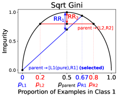
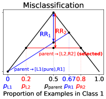
Figure 8: Left: NE loss with $\lambda=0$ ranks the split producing a pure child node above the one that does not. Right: NE loss with $\lambda=1$ gives opposite rankings.

Note that the black curve plots the impurity for a node with a class distribution $(p,1-p)$ against $p$. We use the following trick to read the risk reduction from the plot: consider a node with a class distribution $(p_{\text{parent}},1-p_{\text{parent}})$ and a split which creates two child nodes with class distributions ${\color[rgb]{0,0,1}(p_{L},1-p_{L})}$ and ${\color[rgb]{1,0,0}(p_{R},1-p_{R})}$. Let $A$ and $B$ be the two points of the impurity curve at $p_{L}$ and $p_{R}$, then the risk reduction is the gap between the impurity curve and the line segment $AB$, at $p=p_{\text{parent}}$.

References

• Audubon Society Field Guide (1987) Audubon Society Field Guide. 1987. Mushroom. UCI Machine Learning Repository. DOI: https://doi.org/10.24432/C5959T.
• Blackard (1998) Blackard, J. 1998. Covertype. UCI Machine Learning Repository. DOI: https://doi.org/10.24432/C50K5N.
• Breiman (2001) Breiman, L. 2001. Random forests. Machine learning, 45: 5–32.
• Breiman et al. (1984) Breiman, L.; Friedman, J. H.; Olshen, R. A.; and Stone, C. J. 1984. Classification and regression trees. Wadsworth statistics/probability series. Belmont, Calif.: Wadsworth International Group. ISBN 0534980538.
• Brodley, Friedl et al. (1996) Brodley, C. E.; Friedl, M. A.; et al. 1996. Identifying and eliminating mislabeled training instances. In Proceedings of the National Conference on Artificial Intelligence, 799–805.
• Chang and Lin (2011) Chang, C.-C.; and Lin, C.-J. 2011. LIBSVM: a library for support vector machines. ACM transactions on intelligent systems and technology (TIST), 2(3): 1–27.
• Collobert, Bengio, and Bengio (2001) Collobert, R.; Bengio, S.; and Bengio, Y. 2001. A parallel mixture of SVMs for very large scale problems. Advances in Neural Information Processing Systems, 14.
• Frénay and Verleysen (2013) Frénay, B.; and Verleysen, M. 2013. Classification in the presence of label noise: a survey. IEEE transactions on neural networks and learning systems, 25(5): 845–869.
• Geurts, Ernst, and Wehenkel (2006) Geurts, P.; Ernst, D.; and Wehenkel, L. 2006. Extremely randomized trees. Machine learning, 63: 3–42.
• Ghosh, Kumar, and Sastry (2017) Ghosh, A.; Kumar, H.; and Sastry, P. S. 2017. Robust Loss Functions under Label Noise for Deep Neural Networks. Proceedings of the AAAI Conference on Artificial Intelligence, 31(1).
• Ghosh, Manwani, and Sastry (2015) Ghosh, A.; Manwani, N.; and Sastry, P. 2015. Making risk minimization tolerant to label noise. Neurocomputing, 160: 93–107.
• Ghosh, Manwani, and Sastry (2017) Ghosh, A.; Manwani, N.; and Sastry, P. 2017. On the robustness of decision tree learning under label noise. In Advances in Knowledge Discovery and Data Mining: 21st Pacific-Asia Conference, PAKDD 2017, Jeju, South Korea, May 23-26, 2017, Proceedings, Part I 21, 685–697. Springer.
• Grinsztajn, Oyallon, and Varoquaux (2022) Grinsztajn, L.; Oyallon, E.; and Varoquaux, G. 2022. Why do tree-based models still outperform deep learning on typical tabular data? Advances in Neural Information Processing Systems, 35: 507–520.
• Kaggle (2021) Kaggle. 2021. State of Machine Learning and Data Science 2021.
• Kim et al. (2019) Kim, Y.; Yim, J.; Yun, J.; and Kim, J. 2019. Nlnl: Negative learning for noisy labels. In Proceedings of the IEEE/CVF international conference on computer vision, 101–110.
• Kiryo et al. (2017) Kiryo, R.; Niu, G.; Du Plessis, M. C.; and Sugiyama, M. 2017. Positive-unlabeled learning with non-negative risk estimator. Advances in neural information processing systems, 30.
• Krizhevsky (2009) Krizhevsky, A. 2009. Learning multiple layers of features from tiny images. MSc thesis, University of Toronto.
• Lang (1995) Lang, K. 1995. Newsweeder: Learning to filter netnews. In Machine learning proceedings 1995, 331–339. Elsevier.
• LeCun et al. (1998) LeCun, Y.; Bottou, L.; Bengio, Y.; and Haffner, P. 1998. Gradient-based learning applied to document recognition. Proceedings of the IEEE, 86(11): 2278–2324.
• Lukasik et al. (2020) Lukasik, M.; Bhojanapalli, S.; Menon, A.; and Kumar, S. 2020. Does label smoothing mitigate label noise? In International Conference on Machine Learning, 6448–6458. PMLR.
• Lyu and Tsang (2020) Lyu, Y.; and Tsang, I. W. 2020. Curriculum Loss: Robust Learning and Generalization against Label Corruption. In International Conference on Learning Representations.
• Ma et al. (2020) Ma, X.; Huang, H.; Wang, Y.; Romano, S.; Erfani, S.; and Bailey, J. 2020. Normalized loss functions for deep learning with noisy labels. In International conference on machine learning, 6543–6553. PMLR.
• Mantas and Abellan (2014) Mantas, C. J.; and Abellan, J. 2014. Credal-C4. 5: Decision tree based on imprecise probabilities to classify noisy data. Expert Systems with Applications, 41(10): 4625–4637.
• Manwani and Sastry (2013) Manwani, N.; and Sastry, P. 2013. Noise tolerance under risk minimization. IEEE transactions on cybernetics, 43(3): 1146–1151.
• Moustafa and Slay (2015) Moustafa, N.; and Slay, J. 2015. UNSW-NB15: a comprehensive data set for network intrusion detection systems (UNSW-NB15 network data set). In 2015 military communications and information systems conference (MilCIS), 1–6. IEEE.
• Natarajan et al. (2013) Natarajan, N.; Dhillon, I. S.; Ravikumar, P. K.; and Tewari, A. 2013. Learning with noisy labels. Advances in neural information processing systems, 26.
• Painsky and Wornell (2018) Painsky, A.; and Wornell, G. 2018. On the universality of the logistic loss function. In 2018 IEEE International Symposium on Information Theory (ISIT), 936–940. IEEE.
• Patrini et al. (2017) Patrini, G.; Rozza, A.; Krishna Menon, A.; Nock, R.; and Qu, L. 2017. Making deep neural networks robust to label noise: A loss correction approach. In Proceedings of the IEEE conference on computer vision and pattern recognition, 1944–1952.
• Pedregosa et al. (2011) Pedregosa, F.; Varoquaux, G.; Gramfort, A.; Michel, V.; Thirion, B.; Grisel, O.; Blondel, M.; Prettenhofer, P.; Weiss, R.; and Dubourg, V. 2011. Scikit-learn: Machine learning in Python. the Journal of machine Learning research, 12: 2825–2830.
• Pennington, Socher, and Manning (2014) Pennington, J.; Socher, R.; and Manning, C. D. 2014. GloVe: Global Vectors for Word Representation. In Empirical Methods in Natural Language Processing (EMNLP), 1532–1543.
• Song et al. (2022) Song, H.; Kim, M.; Park, D.; Shin, Y.; and Lee, J.-G. 2022. Learning from noisy labels with deep neural networks: A survey. IEEE Transactions on Neural Networks and Learning Systems.
• Tanno et al. (2019) Tanno, R.; Saeedi, A.; Sankaranarayanan, S.; Alexander, D. C.; and Silberman, N. 2019. Learning from noisy labels by regularized estimation of annotator confusion. In Proceedings of the IEEE/CVF conference on computer vision and pattern recognition, 11244–11253.
• Wang et al. (2019) Wang, Y.; Ma, X.; Chen, Z.; Luo, Y.; Yi, J.; and Bailey, J. 2019. Symmetric cross entropy for robust learning with noisy labels. In Proceedings of the IEEE/CVF international conference on computer vision, 322–330.
• Wilton et al. (2022) Wilton, J.; Koay, A.; Ko, R.; Xu, M.; and Ye, N. 2022. Positive-Unlabeled Learning using Random Forests via Recursive Greedy Risk Minimization. Advances in Neural Information Processing Systems, 35: 24060–24071.
• Yang, Gao, and Li (2019) Yang, B.-B.; Gao, W.; and Li, M. 2019. On the robust splitting criterion of random forest. In 2019 IEEE International Conference on Data Mining (ICDM), 1420–1425. IEEE.
• Zhang and Sabuncu (2018) Zhang, Z.; and Sabuncu, M. 2018. Generalized cross entropy loss for training deep neural networks with noisy labels. Advances in neural information processing systems, 31.
• Zhou, Ding, and Li (2019) Zhou, X.; Ding, P. L. K.; and Li, B. 2019. Improving robustness of random forest under label noise. In 2019 IEEE Winter Conference on Applications of Computer Vision (WACV), 950–958. IEEE.