Robustly Improving Bandit Algorithms with Confounded and Selection Biased Offline Data: A Causal Approach

Wen Huang, Xintao Wu
Abstract

This paper studies bandit problems where an agent has access to offline data that might be utilized to potentially improve the estimation of each arm’s reward distribution. A major obstacle in this setting is the existence of compound biases from the observational data. Ignoring these biases and blindly fitting a model with the biased data could even negatively affect the online learning phase. In this work, we formulate this problem from a causal perspective. First, we categorize the biases into confounding bias and selection bias based on the causal structure they imply. Next, we extract the causal bound for each arm that is robust towards compound biases from biased observational data. The derived bounds contain the ground truth mean reward and can effectively guide the bandit agent to learn a nearly-optimal decision policy. We also conduct regret analysis in both contextual and non-contextual bandit settings and show that prior causal bounds could help consistently reduce the asymptotic regret.

Introduction

The past decade has seen the rapid development of contextual bandit as a legit framework to model interactive decision-making scenarios, such as personalized recommendation (Li et al. 2010), online advertising (Tang et al. 2013; Avadhanula et al. 2021), and anomaly detection (Ding, Li, and Liu 2019). The key challenge in a contextual bandit problem is to select the most beneficial item (i.e. the corresponding arm or intervention) according to the observed context at each round. In practice it is common that the agent has additional access to logged data from various sources, which may provide some useful information. A key issue is how to accurately leverage offline data such that it can efficiently assist the online decision-making process. However, one inevitable problem is that there may exist compound biases in the offline dataset, probably due to the data collection process, the existence of unobserved variables, the policies implemented by the agent, and so on (Chen et al. 2023). As a consequence, blindly fitting a model without considering those biases will lead to an inaccurate estimator of the reward distribution for each arm, ending up inducing a negative impact on the online learning phase.

To overcome this limitation and make good use of the offline data for online bandit learning, we formulate our framework from a causal inference perspective. Causal inference provides a family of methods to infer the effects of actions from a combination of data and qualitative assumptions about the underlying mechanism. Based on Pearl’s structural causal model (Pearl 2009) we can derive a truncated factorization formula that expresses the target causal quantity with probability distributions from the data. Appropriately adopting that prior knowledge on the reward distribution of each arm can accelerate the learning speed and achieve lower cumulative regret for online bandit algorithms.

Previous studies along this direction (Zhang and Bareinboim 2017; Sharma et al. 2020; Tennenholtz et al. 2021) only focused on one specific bias and have not dealt with compound biases in the offline data. It was shown in (Bareinboim, Tian, and Pearl 2014) that biases could be classified into confounding bias and selection bias based on the causal structure they imply. Due to the orthogonality of confounding and selection bias, simply deconfounding and estimating causal effects in the presence of selection bias using observational data is in general impractical without further assumptions, such as strong graphical conditions (Correa and Bareinboim 2017) or the accessibility of external unbiasedly measured data (Bareinboim and Tian 2015). In this paper, we address this limitation by non-parametrically bounding the target conditional causal effect when confounding and selection biases can not be mitigated simultaneously. We propose two novel strategies to extract prior causal bounds for the reward distribution of each arm and use them to effectively guide the bandit agent to learn a nearly-optimal decision policy. We demonstrate that our approach could further reduce cumulative regret and is resistant to different levels of compound biases in offline data.

Our contributions can be summarized into three parts: 1) We derive causal bounds for conditional causal effects under confounding and selection biases based on c-component factorization and substitute intervention methods; 2) we propose a novel framework that leverages the prior causal bound obtained from biased offline data to guide the arm-picking process in bandit algorithms, thus robustly decreasing the exploration of sub-optimal arms and reducing the cumulative regret; and 3) we develop one contextual bandit algorithm (LinUCB-PCB) and one non-contextual bandit algorithm (UCB-PCB) that are enhanced with prior causal bounds. We theoretically show under mild conditions both bandit algorithms achieve lower regret than their non-causal counterparts. We also conduct an empirical evaluation to demonstrate the effectiveness of our method under the linear contextual bandit setting.

Background

Our work is based on Pearl’s structural causal model (Pearl 2009) which describes the causal mechanisms of a system as a set of structural equations.

Definition 1 (Structural Causal Model (SCM) (Pearl 2009)).

A causal model $\mathcal{M}$ is a triple $\mathcal{M}=\langle\mathbf{U},\mathbf{V},\mathbf{F}\rangle$ where 1) $\mathbf{U}$ is a set of hidden contextual variables that are determined by factors outside the model; 2) $\mathbf{V}$ is a set of observed variables that are determined by variables in $\mathbf{U}\cup\mathbf{V}$; 3) $\mathbf{F}$ is a set of equations mapping from $\mathbf{U}\times\mathbf{V}$ to $\mathbf{V}$. Specifically, for each $V\in\mathbf{V}$, there is an equation $v=f_{V}(Pa(V),\mathbf{u}_{V})$ where $Pa(V)$ is a realization of a set of observed variables called the parents of $V$, and $\mathbf{u}_{V}$ is a realization of a set of hidden variables.

Quantitatively measuring causal effects is facilitated with the $do$-operator (Pearl 2009), which simulates the physical interventions that force some variables to take certain values. Formally, the intervention that sets the value of $X$ to $x$ is denoted by $do(x)$. In a SCM, intervention $do(x)$ is defined as the substitution of equation $x=f_{X}(Pa(X),\mathbf{u}_{X})$ with constant $X=x$. The causal model $\mathcal{M}$ is associated with a causal graph $\mathcal{G}=\langle\mathcal{V},\mathcal{E}\rangle$. Each node of $\mathcal{V}$ corresponds to a variable of $\mathbf{V}$ in $\mathcal{M}$. Each edge in $\mathcal{E}$, denoted by a directed arrow $\rightarrow$, points from a node $X\in\mathbf{U}\cup\mathbf{V}$ to a different node $Y\in\mathbf{V}$ if $f_{Y}$ uses values of $X$ as input. The intervention that sets the value of a set of variables $\mathbf{X}$ to $\mathbf{x}$ is denoted by $do(\mathbf{X}=\mathbf{x})$. The post-intervention distribution of the outcome variables $P(\mathbf{y}|do(\mathbf{x}))$ can be computed by the truncated factorization formula (Pearl 2009),

$$P(\mathbf{y}|do(\mathbf{x}))=\prod_{Y\in\mathbf{Y}}P(y|Pa(Y))\delta_{\mathbf{X}=\mathbf{x}},$$ (1)

where $\delta_{\mathbf{X}=\mathbf{x}}$ means assigning attributes in $\mathbf{X}$ involved in the term ahead with the corresponding values in $\mathbf{x}$. The post intervention distribution $P(\mathbf{y}|do(\mathbf{x}))$ is identifiable if it can be uniquely computed from observational distributions $P(\mathbf{V})$.

Confounding Bias occurs when there exist hidden variables that simultaneously determine exposure variables and the outcome variable. It is well known that, in the absence of hidden confounders, all causal effects can be estimated consistently from non-experimental data. However, in the presence of hidden confounders, whether the desired causal quantity can be estimated depends on the locations of the unmeasured variables, the intervention set, and the outcome. To adjust for confounding bias, one common approach is to condition on a set of covariates that satisfy the backdoor criterion. (Shpitser, VanderWeele, and Robins 2012) further generalized the backdoor criterion to identify the causal effect $P(\mathbf{y}|do(\mathbf{x}))$ if all non-proper causal paths are blocked.

Definition 2 (Generalized Backdoor Criterion (Shpitser, VanderWeele, and Robins 2012)).

A set of variables $\mathbf{\mathbf{Z}}$ satisfies the adjustment criterion relative to $(\mathbf{X},\mathbf{Y})$ in $\mathcal{G}$ if: (i) no element in $\mathbf{Z}$ is a descendant in $\mathcal{G}_{\overline{\mathbf{X}}}$ of any $W\notin\mathbf{X}$ lying on a proper causal path from $\mathbf{X}$ to $Y$. (ii) all non-causal paths in $\mathcal{G}$ from $\mathbf{X}$ to $Y$ are blocked by $\mathbf{Z}$.

In Definition 2 $\mathcal{G}_{\overline{\mathbf{X}}}$ denotes the graph resulting from removing all incoming edges to $\mathbf{X}$ in $\mathcal{G}$, and a causal path from a node in $\mathbf{X}$ to $\mathbf{Y}$ is called proper if it does not intersect $\mathbf{X}$ except at the starting point. The causal effect can thus be computed by controlling for a set of covariates $\mathbf{Z}$.

$$P(\mathbf{y}|do(\mathbf{x}))=\sum_{\mathbf{Z}}P(\mathbf{y}|\mathbf{x},\mathbf{z})P(\mathbf{z})$$ (2)

Sample Selection Bias arises with a biased selection mechanism, e.g., choosing users based on a certain time or location. To accommodate for SCM framework, we introduce a node $S$ in a causal graph representing a binary indicator of entry into the observed data, and denote the causal graph augmented with selection node $S$ as $\mathcal{G}_{s}$. Generally speaking, the target distribution $P(\mathbf{y}|do(\mathbf{x}))$ is called s-recoverable if it can be computed from the available (biased) observational distributions $P(\mathbf{V}|S=1)$ in the augmented graph $\mathcal{G}_{s}$. To recover causal effects in the presence of confounding and sample selection bias, (Correa, Tian, and Bareinboim 2018) studied the use of generalized adjustment criteria and introduced a sufficient and necessary condition for recovering causal effects from biased distributions.

Theorem 1 (Generalized Adjustment for Causal Effect (Correa, Tian, and Bareinboim 2018)).

Given a causal diagram $\mathcal{G}$ augmented with selection variable $S$, disjoint sets of variables $\mathbf{Y},\mathbf{X},\mathbf{Z}$, for every model compatible with $\mathcal{G}$, we have

$$P(\mathbf{y}|do(\mathbf{x}))=\sum_{\mathbf{Z}}P(\mathbf{y}|\mathbf{x},\mathbf{z},S=1)P(\mathbf{z}|S=1)$$ (3)

if and only if the adjustment variable set $\mathbf{Z}$ satisfies the four criterion shown in (Correa, Tian, and Bareinboim 2018).

Instead of identifying causal effect in presence of selection bias by adjustment, (Correa, Tian, and Bareinboim 2019) proposed a parallel procedure to justify whether a causal quantity is identifiable and recoverable from selection bias using axiomatical c-components factorization (Tian and Pearl 2002). However, both techniques require strong graphical condition to obtain the unbiased estimation of the true conditional causal effect when both confounding and selection biases exist.

Basically, c-component factorization first partitions nodes in $\mathcal{G}$ into a set of c-components, then expresses the target intervention in terms of the c-factors corresponding to each c-component. Specifically, a c-component $\bm{C}$ denotes a subset of variables in $\mathcal{G}$ such that any two nodes in $\bm{C}$ are connected by a path entirely consisting of bi-directed edges. A bi-directed edge indicates there exists unobserved confounder(s) between the two connected nodes. A c-factor $Q[\bm{C}](\mathbf{v})$ is a function that demonstrates the post-intervention distribution of $\bm{C}$ after conducting interventions on the remaining variables $\mathbf{V}\backslash\bm{C}$ and is defined as

$$Q[\bm{C}](\mathbf{v})=P(\bm{c}|do(\mathbf{v}\backslash\bm{c}))=\sum_{\mathbf{U}}\prod_{V\in\bm{C}}P(v|Pa(v),\mathbf{u}_{v})P(\mathbf{u})$$

where $Pa(v)$ and $\mathbf{u}_{v}$ denote the set of observed and unobserved parents for node $V$. We explicitly denote $Q[\bm{C}](\mathbf{v})$ as $Q[\bm{C}]$ and list the factorization formula.

Theorem 2 (C-component Factorization (Tian and Pearl 2002)).

Given a causal graph $\mathcal{G}$, the target intervention $P(\mathbf{y}|do(\mathbf{x}))$ could be expressed as a product of c-factors associated with the c-components as follows:

$$P(\mathbf{y}|do(\mathbf{x}))=\sum_{\bm{C}\backslash\mathbf{Y}}Q[\bm{C}]=\sum_{\bm{C}\backslash\mathbf{Y}}\prod_{i=1}^{l}Q[\bm{C}_{i}]$$ (4)

where $\mathbf{X},\mathbf{Y}\subset\mathbf{V}$ could be arbitrary sets, $\bm{C}=An(\mathbf{Y})_{\mathcal{G}_{\mathbf{V}\backslash\mathbf{X}}}$ denotes the ancestor node set of $\mathbf{Y}$ in sub-graph $\mathcal{G}_{\mathbf{V}\backslash\mathbf{X}}$, and $\bm{C}_{1},...,\bm{C}_{l}$ are the c-components of $\mathcal{G}_{\bm{C}}$.

(Bareinboim, Tian, and Pearl 2014) showed that $P(\mathbf{y}|do(\mathbf{x}))$ is recoverable and could be computed by Equation 4 if each factor $Q[\bm{C}_{i}]$ is recoverable from the observational data. Accordingly, they developed the RC algorithm to determine the recoverability of each c-factor.

Related Works

Causal Inference under Confounding and Selection Biases. (Bareinboim, Tian, and Pearl 2014) firstly studied the use of covariate adjustment for simultaneously dealing with both confounding and selection biases based on the SCM. (Correa and Bareinboim 2017) developed a set of complete conditions to recover causal effects in two cases: when none of the covariates are measured externally, and when all of them are measured without selection bias. (Correa, Tian, and Bareinboim 2018) further studied a general case when only a subset of the covariates require external measurement. They developed adjustment-based technique that combines the partial unbiased data with the biased data to produce an estimand of the causal effect in the overall population. Different from these works that focus on recovering causal effects under certain graph conditions, our work focuses on bounding causal effects under compound biases, which is needed in various application domains.

Combining Offline Evaluation and Online Learning in Bandit Setting. Recently there are research works that focus on confounding issue in bandit setting (Bareinboim, Forney, and Pearl 2015; Tennenholtz et al. 2021). It is shown in (Bareinboim, Forney, and Pearl 2015) that in MAB problems, neglecting unobserved confounders will lead to a sub-optimal arm selection strategy. They also demonstrated that one can not simulate the optimal arm-picking strategy by a single data collection procedure, such as pure offline or online evaluation. To this end, another line of research works considers combining offline causal inference techniques and online bandit learning to approximate a nearly-optimal policy. (Tennenholtz et al. 2021) studied a linear bandit problem where the agent is provided with partially observed offline data. (Zhang and Bareinboim 2017, 2021) derived causal bounds based on structural causal model and used them to guide arm selection in online bandit algorithms. (Sharma et al. 2020) further leveraged the information provided by the lower bound of the mean reward to reduce the cumulative regret. Nevertheless, none of the bounds derived by these methods are based on a feature-level causal graph extracted from the offline data. (Li et al. 2021; Tang and Xie 2021) proposed another direction to unify offline causal inference and online bandit learning by extracting appropriate logged data and feed it to online learning phase. Their VirUCB-based framework mitigates the cold start problem and can thus boost the learning speed for a bandit algorithm without any cost on the regret. However, none of those proposed algorithms take selection bias and confounding bias simultaneously into consideration during offline evaluation phase.

Algorithm Framework

An overview of our framework is illustrated in Figure 1. Our algorithm framework leverages the observational data to derive a prior causal bound for each arm to mitigate the cold start issue in online bandit learning, thus reducing the cumulative regret. In the offline evaluation phase, we call our bounding conditional causal effect (BCE) algorithm (shown in Algorithm 1) to obtain the prior causal bound for each arm given a user’s profile. Then in the online bandit phase, we apply adapted contextual bandit algorithms with the prior causal bounds as input.
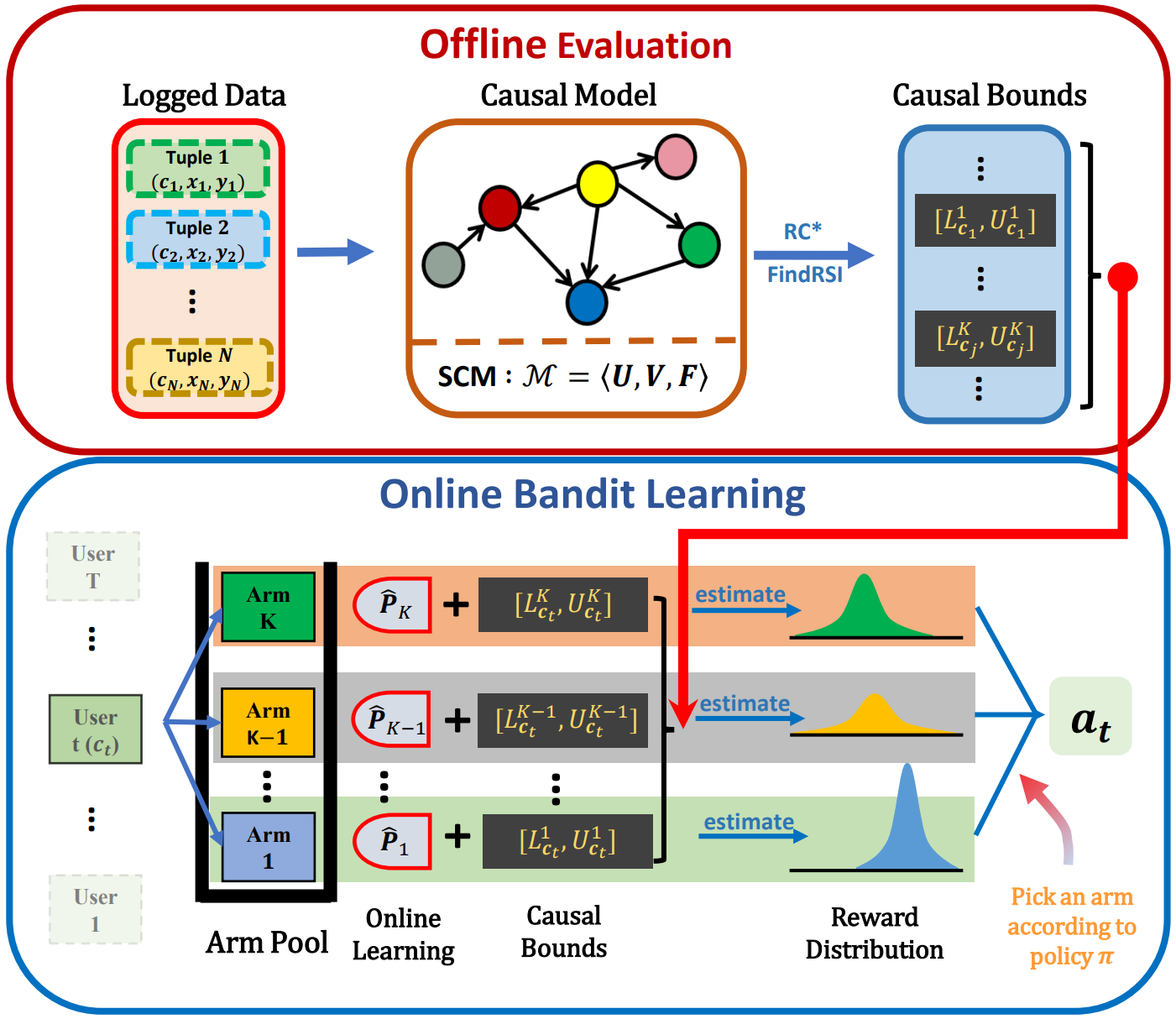
Refer to caption
Figure 1: An illustration graph of our proposed framework.

Let $\mathbf{C}\in\mathcal{C}$ denote the context vector, where $\mathcal{C}$ denotes the domain space of $\mathbf{C}$. We use $Y$ to denote the reward variable and $\mathbf{X}\in\mathcal{X}$ to denote the intervention variables. At each time $t\in[T]$, a user arrives and the user profile $\mathbf{c}_{t}$ is revealed to the agent. The agent pulls an arm $a_{t}$ with features $\mathbf{x}_{a_{t}}$ based on previous observations. The agent then receives the reward $Y_{t}$ and observes values for all non-intervened variables. We define the the expected mean reward of pulling an arm $a$ with with feature value $\mathbf{x}_{a}$ given user context $\mathbf{c}$ as the conditional causal effect shown below:

$$u_{a,\mathbf{c}}=\mathbb{E}[Y|do(\mathbf{X}=\mathbf{x}_{a}),\mathbf{c}]$$ (5)

When the offline data are available, we can leverage them as prior estimators of the reward for each arm to reduce explorations in the online phase. However, under the circumstances that the causal effect is either unidentifiable or nonrecoverable from the observational data, blindly using the observational data might even have a negative effect on the online learning phase. Our approach is to derive a causal bound for the desired causal effect from the biased observational data. We will further show even when the observational data could only lead to loose causal bounds, we can still guarantee our approach is no worse than conventional bandit algorithms.

Deriving Causal Bounds under Confounding and Selection Biases

In this section, we focus on bounding the effects of conditional interventions in the presence of confounding and sample selection biases. To tackle the identifiability issue of a conditional intervention $P(Y=y|do(\mathbf{x}),\mathbf{c})$, the cond-identify algorithm (Tian 2004) provides a complete procedure to compute conditional causal effects using observational distributions.

$$P(Y=y|do(\mathbf{x}),\mathbf{c})=P_{\mathbf{x}}(y|\mathbf{c})=\frac{P_{\mathbf{x}}(y,\mathbf{c})}{P_{\mathbf{x}}(\mathbf{c})}$$ (6)

where $P_{\mathbf{x}}(y|\mathbf{c})$ is the abbreviated form of the conditional causal effect $P(Y=y|do(\mathbf{x}),\mathbf{c})$. (Tian 2004) showed that if the numerator $P_{\mathbf{x}}(y,\mathbf{c})$ is identifiable, then $P_{\mathbf{x}}(y|\mathbf{c})$ is also identifiable. In the contextual bandit setting, because none of the variables in $\mathbf{C}$ is a descendant of variables in $\mathbf{X}$, the denominator $P_{\mathbf{x}}(\mathbf{c})$ can be reduced to $P(\mathbf{c})$ following the causal topology. Since $P(\mathbf{c})$ is always identifiable and can be accurately estimated, we do not need to consider the situation where neither $P_{\mathbf{x}}(y,\mathbf{c})$ nor $P_{\mathbf{x}}(\mathbf{c})$ is identifiable but $P_{\mathbf{x}}(y|\mathbf{c})$ is still identifiable. Thus the conditional causal effect $P_{\mathbf{x}}(y|\mathbf{c})$ in Equation 6 is identifiable if and only if $P_{\mathbf{x}}(y,\mathbf{c})$ is identifiable. However, the cond-identify algorithm (Tian 2004) is not applicable for the scenario with the presence of selection bias.

Algorithm 1 shows our algorithm framework of bounding conditional causal effects under confounding and selection biases. We develop two methods, c-component factorization and substitute intervention, and apply each to derive a bound for conditional causal effect separately. We then compare the two causal bounds and return the tighter upper/lower bound. Specifically, lines 5-10 in Algorithm 1 decompose the target causal effect following c-component factorization and recursively call our RC* algorithm (shown in Algorithm 2) to bound each c-factor. Lines 11-15 search over recoverable intervention space and find valid substitute interventions to bound the target causal effect. Lines 16-18 compare two derived causal bounds and take the tighter upper/lower bound as the output causal bounds. We also include discussions regarding the assumptions on causal graph in Appendix.

Algorithm 1 Bounding Conditional Causal Effect
1:  function BCE$(\mathbf{x},\mathbf{c},y,\mathcal{G},\mathcal{H})$
2:  Input: Intervention variables $\mathbf{X}=\mathbf{x}$, context vector $\mathbf{C}=\mathbf{c}$, outcome variable $Y=y$, causal graph $\mathcal{G}$.
3:  Output: Causal bound $[L_{\mathbf{x},\mathbf{c}},U_{\mathbf{x},\mathbf{c}}]$ of the conditional intervention $P_{\mathbf{x}}(y|\mathbf{c})$.
4:  Initialization: $[L_{q},U_{q}]=[0,1],[L_{w},U_{w}]=[0,1]$
5:  // C-component Factorization
6:  Decompose $P_{\mathbf{x}}(y,\mathbf{c})=\sum_{\mathbf{D}\backslash\{\mathbf{Y},\mathbf{C}\}}\prod_{i=1}^{l}Q[\mathbf{D}_{i}]$ following Equation 4.
7:  for each $\mathbf{D}_{i}$ do
8:     $L_{Q(\mathbf{D}_{i})},U_{Q(\mathbf{D}_{i})}=\text{RC*}(\mathbf{D}_{i},P(\mathbf{v}|S=1),\mathcal{G})$
9:  end for
10:  Update $L_{q},U_{q}$ according to Theorem 7.
11:  // Substitute Intervention
12:  $\mathcal{D}=\text{FindRSI}(\mathbf{x},\mathbf{c},y,\mathcal{G})$
13:  if $\mathcal{D}\neq\phi$ then
14:     Update $L_{w},U_{w}$ according to Theorem 10.
15:  end if
16:  // Comparing Bounds
17:  Calculate estimated values $\hat{L}_{q},\hat{L}_{w},\hat{U}_{q},\hat{U}_{w}$ based on $\mathcal{H}$.
18:  return  $L_{\mathbf{x},\mathbf{c}}=\max\{\hat{L}_{q},\hat{L}_{w}\}$, $U_{\mathbf{x},\mathbf{c}}=\min\{\hat{U}_{q},\hat{U}_{w}\}$

Bounding via C-component Factorization

To derive the causal bound based on c-component factorization, we decompose the target intervention into c-factors and call RC* algorithm to recover each c-factor. The RC* algorithm shown in Algorithm 2 is designed based on the RC algorithm in (Correa, Tian, and Bareinboim 2019) to accommodate for non-recoverable situations. When the c-factor $Q[\mathbf{E}]$ is recoverable, the RC* algorithm returns an expression of $Q[\mathbf{E}]$ using biased distribution $P(\mathbf{v}|S=1)$.

Specifically, lines 4-6 in Algorithm 2 marginalize out the non-ancestors of $\mathbf{E}\cup S$ since they do not affect the recoverability results. From Lemma 3 in (Bareinboim and Tian 2015), each c-component in line 7 is recoverable since none of them contains ancestors of $S$. Line 13 calls the Identify function proposed by (Tian and Pearl 2003) that gives a complete procedure to determine the identifiability of $Q[\mathbf{E}]$. When $Q[\mathbf{E}]$ is identifiable, $\text{Identify}(\mathbf{E},\bm{C}_{i},Q[\bm{C}_{i}])$ returns a closed form expression of $Q[\mathbf{E}]$ in terms of $Q[\bm{C}_{i}]$. In line 15, if none of the recoverable c-components $\bm{C}_{i}$ contains $\mathbf{E}$, we replace the distribution $P$ by dividing the recoverable quantity $\prod_{i}Q[\bm{C}_{i}]$ and recursively run the RC* algorithm on the graph $\mathcal{G}_{\mathbf{V}\backslash\bm{C}}$. Under certain situations where line 8 in RC* Algorithm fails ($\bm{C}=\emptyset$), the corresponding $Q[\mathbf{E}]$ can not be computed from the biased observational data in theory. These situations are referred to as nonrecoverable situations. We address this nonrecoverable challenge by non-parametrically bounding the targeted causal quantity. In this case, RC* returns a bound $[L_{Q(\mathbf{E})},U_{Q(\mathbf{E})}]$ for $Q[\mathbf{E}]$. The bound for $P_{\mathbf{x}}(y,\mathbf{c})$ is derived by summing up the estimator/bounds of those c-factors following Equation 4.

Algorithm 2 RC* Algorithm
1:  function RC*$(\mathbf{E},P,\mathcal{G})$
2:  Input: $\mathbf{E}$ a c-component, $P$ a distribution and $\mathcal{G}$ a causal graph.
3:  Output: Causal bound $[L_{Q[\mathbf{E}]},U_{Q(\mathbf{E})}]$ for $Q[\mathbf{E}]$.
4:  if $\mathbf{V}\backslash(An(\mathbf{E})\cup An(S))\neq\phi$ then
5:     return  RC*$(\mathbf{E},\sum_{\mathbf{V}\backslash(An(\mathbf{E})\cup An(S))}P,\mathcal{G}_{(An(\mathbf{E})\cup An(S))})$
6:  end if
7:  Let $\bm{C}_{1},...,\bm{C}_{k}$ be the c-components of $\mathcal{G}$ that contains no ancestors of $S$ and $\bm{C}=\cup_{i\in[k]}\bm{C}_{i}$.
8:  if $\bm{C}=\emptyset$ then
9:     Bound $Q[\mathbf{E}]$ with $U_{Q(\mathbf{E})}=1,L_{Q(\mathbf{E})}=0$.
10:     return  $L_{Q(\mathbf{E})},U_{Q(\mathbf{E})}$
11:  end if
12:  if $\mathbf{E}$ is a subset of some $\bm{C}_{i}$ and $\text{Identify}(\mathbf{E},\bm{C}_{i},Q[\bm{C}_{i}])$ does not return FAIL then
13:     return  $L_{Q(\mathbf{E})}=U_{Q(\mathbf{E})}=\text{Identify}(\mathbf{E},\bm{C}_{i},Q[\bm{C}_{i}])$
14:  end if
15:  return  RC*$(\mathbf{E},\frac{P}{\prod_{i}Q[\bm{C}_{i}]},\mathcal{G}_{\mathbf{V}\backslash\bm{C}})$

Note that in line 9 of RC* algorithm, we bound the target c-component by $[0,1]$ since under semi-Markovian models it is challenging to find a tight bound for $Q[\mathbf{E}]$ when $\bm{C}=\emptyset$. One future direction is to further apply a non-parametric bounding technique similar to (Wu, Zhang, and Wu 2019). That is, choosing certain probability distributions in the truncated formula that are the source of unrecoverability, and set specific domain values for a carefully chosen variable set to allow these distributions achieve their maximum/minimum values. Finally we list the causal bounds derived from calling RC* algorithm in the follow Theorem:

Theorem 3 (Causal Bound from RC* algorithm).

Given a conditional intervention $P_{\mathbf{x}}(y|\mathbf{c})$, the causal bounds derived by calling RC* algorithm for each c-factor are:

$$\begin{split}L_{q}=\sum_{\mathbf{D}\backslash\{\mathbf{Y},\mathbf{C}\}}\prod_{i=1}^{l}L_{Q[D_{i}]}/P_{\mathbf{x}}(\mathbf{c})\\ U_{q}=\sum_{\mathbf{D}\backslash\{\mathbf{Y},\mathbf{C}\}}\prod_{i=1}^{l}U_{Q[D_{i}]}/P_{\mathbf{x}}(\mathbf{c})\end{split}$$ (7)

Bounding via Substitute Interventions

From previous discussion we find that RC* algorithm may return a loose bound when we fail to recover most of the c-factors. In order to obtain a tight causal bound that is robust under various graph conditions, we develop another novel strategy to bound $P_{\mathbf{x}}(y,\mathbf{c})$. Our key idea is to search over the substitute recoverable interventions with a larger intervention space. Note that for a variable set $\mathbf{W}$ such that $\mathbf{W}\cap\mathbf{X}=\emptyset$ in the contextual bandit setting, we can perform marginalization on $\mathbf{W}$ and derive $P_{\mathbf{x}}(y,\mathbf{c})=\sum_{\mathbf{\mathbf{W}}}P_{\mathbf{x}}(y,\mathbf{c}|\mathbf{w})P(\mathbf{w})$. We can further bound $P_{\mathbf{x}}(y,\mathbf{c})$ by

$$\begin{split}P_{\mathbf{x}}(y,\mathbf{c})\leq\max\limits_{\mathbf{w}^{*}\in\mathbf{W}}P_{\mathbf{x}}(y,\mathbf{c}|\mathbf{w}^{*})\\ P_{\mathbf{x}}(y,\mathbf{c})\geq\min\limits_{\mathbf{w}^{*}\in\mathbf{W}}P_{\mathbf{x}}(y,\mathbf{c}|\mathbf{w}^{*})\end{split}$$ (8)

We then investigate whether the action/observation exchange rule of do-calculus (Pearl 2009) and the corresponding graph conditions could be extended in the presence of selection bias and list the results in the following lemma.

Lemma 1 (Action/Observation Rule under Selection Bias).

If the graphical condition $(\mathbf{Y}\mathchoice{\mathrel{\hbox to0.0pt{$\displaystyle\perp$\hss}\mkern 2.0mu{\displaystyle\perp}}}{\mathrel{\hbox to0.0pt{$\textstyle\perp$\hss}\mkern 2.0mu{\textstyle\perp}}}{\mathrel{\hbox to0.0pt{$\scriptstyle\perp$\hss}\mkern 2.0mu{\scriptstyle\perp}}}{\mathrel{\hbox to0.0pt{$\scriptscriptstyle\perp$\hss}\mkern 2.0mu{\scriptscriptstyle\perp}}}\mathbf{Z},S|\mathbf{X},\mathbf{W})_{\mathcal{G}_{\overline{\mathbf{X}}\overline{\mathbf{Z}(\mathbf{w})}}}$ is satisfied in $\mathcal{G}$, the following equivalence between two post-interventional distributions holds:

$$P(\mathbf{y}|do(\mathbf{x}),do(\mathbf{w}),\mathbf{z},S=1)=P(y|do(\mathbf{x}),\mathbf{W},\mathbf{z},S=1)$$ (9)

where $\mathcal{G}_{\overline{\mathbf{X}}\underline{\mathbf{Z}}}$ represents the causal graph with the deletion of both incoming and outgoing arrows of $\mathbf{X}$ and $\mathbf{Z}$ respectively. $\mathbf{Z}(\mathbf{W})$ is the set of $\mathbf{Z}$-nodes that are not ancestors of variables in $\mathbf{W}$ in $\mathcal{G}_{\overline{\mathbf{X}}}$.

Following the general action/observation exchange rules in Equation 9, if $(Y,\mathbf{C}\mathchoice{\mathrel{\hbox to0.0pt{$\displaystyle\perp$\hss}\mkern 2.0mu{\displaystyle\perp}}}{\mathrel{\hbox to0.0pt{$\textstyle\perp$\hss}\mkern 2.0mu{\textstyle\perp}}}{\mathrel{\hbox to0.0pt{$\scriptstyle\perp$\hss}\mkern 2.0mu{\scriptstyle\perp}}}{\mathrel{\hbox to0.0pt{$\scriptscriptstyle\perp$\hss}\mkern 2.0mu{\scriptscriptstyle\perp}}}\mathbf{W},S|\mathbf{X})_{\mathcal{G}_{\overline{\mathbf{X}}\underline{\mathbf{W}}}}$, we can replace $P_{\mathbf{x}}(y,\mathbf{c}|\mathbf{w}^{*})$ with $P_{\mathbf{x},\mathbf{w}^{*}}(y,\mathbf{c})$ and derive the bound for $P_{\mathbf{x}}(y,\mathbf{c})$ as shown in Theorem 10.

Theorem 4 (Causal Bound with Substitute Interventions).

Given a set of variables corresponding to recoverable substitute interventions: $\mathcal{D}=\{\mathbf{W}|P_{\mathbf{x},\mathbf{w}}(y,\mathbf{c})~{}\text{is recoverable}\}$, the target conditional intervention $P_{\mathbf{x}}(y|\mathbf{c})$ is bounded by

$$\begin{split}L_{w}=\max\limits_{\mathbf{W}\in\mathcal{D}}\min\limits_{\mathbf{w}^{*}\in\mathbf{W}}P_{\mathbf{x},\mathbf{w}^{*}}(y,\mathbf{c})/P_{\mathbf{x}}(\mathbf{c})\\ U_{w}=\min\limits_{\mathbf{W}\in\mathcal{D}}\max\limits_{\mathbf{w}^{*}\in\mathbf{W}}P_{\mathbf{x},\mathbf{w}^{*}}(y,\mathbf{c})/P_{\mathbf{x}}(\mathbf{c})\end{split}$$ (10)
Algorithm 3 Finding Recoverable Substitute Interventions
1:  function FindRSI$(\mathbf{x},\mathbf{c},y,\mathcal{G})$
2:  Input: Causal graph $\mathcal{G}$, target intervention $P_{\mathbf{x}}(y,\mathbf{c})$.
3:  Output: A valid variable set $\mathcal{D}=\{\mathbf{W}|P_{\mathbf{x},\mathbf{w}}(y,\mathbf{c})$ is recoverable and could be expressed in terms of biased observational distributions following Equation 3$\}$.
4:  Initialize: $\mathcal{D}\leftarrow\emptyset$.
5:  for all  $\mathbf{W}$ such that $\mathbf{W}\cap\mathbf{X}=\emptyset$, starting with the smallest size of $\mathbf{W}$ do
6:     if a valid adjustment set can be found according to Theorem 1 then
7:        $\mathcal{D}=\mathcal{D}\cup\{\mathbf{W}\}$
8:     end if
9:  end for

We list our procedure of finding all the recoverable substitute interventions in Algorithm 3. Basically the main function FindRSI in Algorithm 3 returns a set containing all admissible variables, each of which corresponding to a recoverable intervention with a larger intervention space.

Next, we give an illustration example on how to run our BCE algorithm to get prior causal bounds. Figure 2 shows a causal graph constructed from offline data, where nodes $U_{1},U_{2}$ and $X_{1},X_{2}$ depict user features and item features respectively, $Y$ denotes the outcome variable, $S$ denotes the selection variable, and $I_{1}$ denotes an intermediate variable. The dashed node $C_{1}$ denotes the confounder that affects both $I_{1}$ and $Y$ simultaneously. To bound the conditional causal effect $p_{x_{1},x_{2}}(y|u_{1},u_{2})$ via c-component factorization, we first identify the set $\mathbf{D}=An(\mathbf{Y})_{\mathcal{G}_{\mathbf{V}\backslash\mathbf{X}}}=\{Y,U_{1},U_{2}\}$. The target intervention could be expressed as

$$\begin{split}p_{x_{1},x_{2}}&(y|u_{1},u_{2})=p_{x_{1},x_{2}}(y,u_{1},u_{2})/p(u_{1},u_{2})\\ &\quad\;\;=(Q[Y]\cdot Q[U_{1}]\cdot Q[U_{2}])/p(u_{1},u_{2})\end{split}$$ (11)

We then call RC* algorithm to bound each c-component and return the bound for each arm according to Theorem 7. For bounding causal effects via substitute interventions, we call FindRSI to find a valid variable set $\mathcal{D}=\{I_{1}\}$. According to Theorem 10, we can obtain the bound for each arm.

$S$ $X_{1}$ $X_{2}$ $U_{1}$ $U_{2}$ $I_{1}$ $C_{1}$ $Y$
Figure 2: Causal graph for synthetic data.

Online Bandit Learning with Prior Causal Bounds

In this section we show how to incorporate our derived causal bounds to online contextual bandit algorithms. We focus on the stochastic contextual bandit setting with linear reward function. We define the concatenation of user and arm feature as $\mathbf{x}_{\mathbf{c}_{t},a}=[\mathbf{c}_{t},\mathbf{x}_{a}]\in\mathbb{R}^{d}$ when the agent picks arm $a$ based on user profile $\mathbf{c}_{t}$ at time $t\in[T]$ and use its simplified notion $\mathbf{x}_{t,a}$ to be consistent with previous work like LinUCB. Under the linear assumption, the binary reward is generated by a Bernoulli distribution $Y_{a}\sim Ber(\langle\bm{\theta},\mathbf{x}_{t,a}\rangle)$ parameterized by $\bm{\theta}$. Let $a_{t}=\operatorname*{arg\,max}_{a\in\mathcal{A}}\mathbb{E}[Y_{a}]$, the expected cumulative regret up to time $T$ is defined as:

$$\mathbb{E}[R(T)]=\sum_{t=1}^{T}\langle\bm{\theta},\mathbf{x}_{t,a^{*}}\rangle-\sum_{t=1}^{T}\mathbb{E}[Y_{a_{t}}]$$

At each round the agent pulls an arm based on the user context, observes the reward, and aims to minimize the expected cumulative regret $\mathbb{E}[R(T)]$ after $T$ rounds. We next conduct regret analysis and show our strategy could consistently reduce the long-term regret with the guide of a prior causal bound for each arm’s reward distribution.

LinUCB algorithm with Prior Causal Bounds

LinUCB (Chu et al. 2011) is one of the most widely used stochastic contextual bandit algorithms that assume the expected reward of each arm $a$ is linearly dependant on its feature vector $\mathbf{x}_{t,a}$ with an unknown coefficient $\bm{\theta}_{a}$ at time $t$. We develop the LinUCB-PCB algorithm that includes a modified arm-picking strategy, clipping the original upper confidence bounds with the prior causal bounds obtained from the offline evaluation phase. Algorithm 4 shows the pseudo-code of our LinUCB-PCB algorithm. The truncated upper confidence bound shown in line 10 of Algorithm 4 contains strong prior information about the true reward distribution implied by the prior causal bound, thus leading to a lower asymptotic regret bound. We include the proof details of Theorem 5 and 6 in Appendix.

Algorithm 4 LinUCB algorithm with Prior Causal Bounds (LinUCB-PCB)
1:  Input: Time horizon $T$, arm set $\mathcal{A}$, prior causal bounds $\{[L_{a,\mathbf{c}},U_{a,\mathbf{c}}]\}_{a,\mathbf{c}\in\{\mathcal{A},\mathcal{C}\}}$, $\alpha$ $\in$ $\mathbb{R}^{+}$.
2:  for t = 1,2,3,…,$T$ do
3:     Observe $\mathbf{x}_{t,a}\in\mathbb{R}^{d}$ for user profile $c_{t}$ and every arm $a$
4:     for $a\in\mathcal{A}$  do
5:        if $a$ is new then
6:           $A_{a}\leftarrow\mathbf{I_{d}}$, $\mathbf{b}_{a}\leftarrow\mathbf{0}_{d\times 1}$
7:        end if
8:        $\bm{\hat{\theta}}_{a}\leftarrow A^{-1}_{a}\mathbf{b}_{a}$
9:        $UCB_{a}(t)\leftarrow\hat{\bm{\theta}}_{a}^{\mathrm{T}}\mathbf{x}_{t,a}+\alpha\sqrt{\mathbf{x}_{t,a}^{\mathrm{T}}A_{a}^{-1}\mathbf{x}_{t,a}}$
10:        $\overline{UCB}_{a}(t)\leftarrow\min\big{\{}UCB_{a}(t),U_{a,\mathbf{c}_{t}}\}$
11:        //Truncated UCB
12:     end for
13:     Pull arm $a_{t}\leftarrow argmax_{a\in\mathcal{A}}\overline{UCB}_{a}(t)$, and observe a reward $r_{t,a_{t}}$
14:     $A_{a_{t}}\leftarrow A_{a_{t}}+\mathbf{x}_{t,a_{t}}\mathbf{x}^{\mathrm{T}}_{t,a_{t}}$, $\mathbf{b}_{a_{t}}\leftarrow\mathbf{b}_{a_{t}}+r_{t,a_{t}}\mathbf{x}_{t,a_{t}}$
15:  end for
Theorem 5.

Let $||\mathbf{x}||_{2}$ define the L-2 norm of a context vector $\mathbf{x}\in\mathbb{R}^{d}$ and

$$L=\max_{a,\mathbf{c}\in\{\mathcal{A},\mathcal{C}\},U_{a,\mathbf{c}}\geq\langle\bm{\theta},\mathbf{x}_{a^{*},\mathbf{c}}\rangle}||\mathbf{x}_{a,\mathbf{c}}||_{2}$$

The expected regret of LinUCB-PCB algorithm is bounded by:

$$\displaystyle\begin{split}R_{T}&\leq\sqrt{2Tdlog(1+TL^{2}/(d\lambda))}\\ &\times 2(\sqrt{\lambda}M+\sqrt{2log(1/\delta)+dlog(1+TL^{2}/(d\lambda))})\end{split}$$

where $M$ denotes the upper bound of $||\bm{\theta}_{a}||_{2}$ for all arms, $\lambda$ denotes the penalty factor corresponding to the ridge regression estimator $\bm{\hat{\theta}}_{a}$.

We follow the standard procedure of deriving the expected regret bound for linear contextual bandit algorithms in (Abbasi-Yadkori, Pál, and Szepesvári 2011) and (Lattimore and Szepesvári 2020). We next discuss the potential improvement in regret that can be achieved by applying LinUCB-PCB algorithm in comparison to original LinUCB algorithm.

Theorem 6.

If there exists an arm $a$ such that $U_{a,\mathbf{c}_{t}}<\langle\bm{\theta},\mathbf{x}_{a^{*},\mathbf{c}_{t}}\rangle$ at a round $t\in[T]$, LinUCB-PCB is guaranteed to achieve lower cumulative regret than LinUCB algorithm.

We further define the total number of sub-optimal arms implied by prior causal bounds as

$$N_{pcb}^{-}=\sum_{a,\mathbf{c}\in\{\mathcal{A},\mathcal{C}\}}\mathds{1}_{U_{a,\mathbf{c}}-\langle\bm{\theta},\mathbf{x}_{a^{*},\mathbf{c}}\rangle<0}$$

Note that the value of $N_{pcb}^{-}$ depends on the accuracy of the causal upper bound for each arm. This is because if the estimated causal bounds are more concentrated, that is, $U_{a,\mathbf{c}}$ is close to $\langle\bm{\theta},\mathbf{x}_{a,\mathbf{c}}\rangle$ for each $a,\mathbf{c}\in\{\mathcal{A},\mathcal{C}\}$, there will be more arms whose prior causal upper bound is less than the optimal mean reward, thus $N_{pcb}^{-}$ will increase accordingly. A large $N_{pcb}^{-}$ value implies less uncertainty regarding the sub-optimal arms implied by prior causal bounds. As a result there are in general less arms to be explored and the $L$ value will decrease accordingly, leading to a more significant improvement by applying LinUCB-PCB algorithm.

Extension We have also investigated leveraging the developed causal bounds to further improve one state-of-the-art contextual bandit algorithm (Hao, Lattimore, and Szepesvari 2020) and one classical non-contextual bandit algorithm (Lattimore and Szepesvári 2020). Due to page limit we defer our developed OAM-PCB and UCB-PCB algorithms as well as the corresponding regret analysis to Appendix.

Empirical Evaluation

In this section, we conduct experiments to validate our proposed methods. We use the synthetic data generated following the graph structure in Figure 2. We generate 30000 data points following the conditional probability table in Appendix to simulate the confounded and selection biased setting. After conducting the preferential exclusion indicated by the selection mechanism, there are approximately 15000 data points used for offline evaluation.

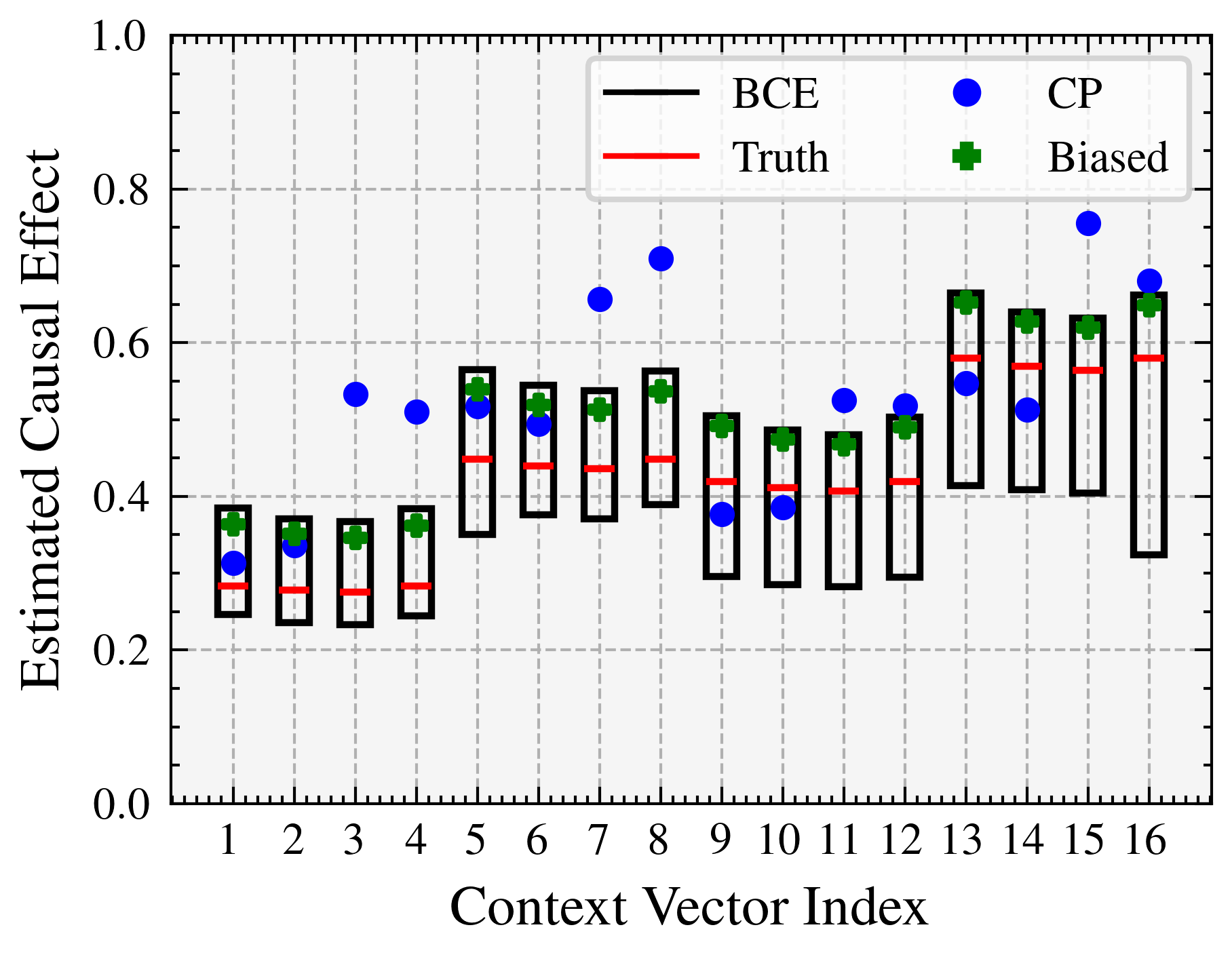
Offline Evaluation We use our BCE algorithm to obtain the bound of each arm based on the input offline data and compare the causal bound derived by the algorithm with the estimated values from two baselines: an estimate that is derived based on Equation 2 which only takes into account confounding bias (Biased), and a naive conditional probability estimate derived without considering both confounding and selection biases (CP). We further report the causal bounds and the estimated reward among 16 different values of the context vector in Figure 3. The comparison results show our BCE algorithm contains the ground-truth causal effect (denoted by the red lines in the figure) for each value of the context vector. On the contrary, the estimated values from CP and Biased baselines deviate from the true causal effect in the presence of compound biases. The experimental results reveal the fact that neglecting any bias will inevitably lead to an inaccurate estimation of the target causal effect.

Refer to caption
Figure 3: Comparison results for offline evaluation under confounding and selection biases.
Refer to caption
Figure 4: Comparison results for contextual linear bandit.

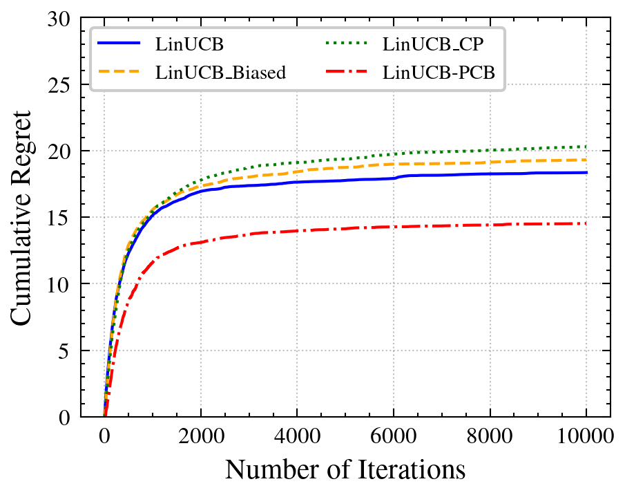
Online Bandit Learning We use 15000 samples from the generated data to simulate the online bandit learning process. In Figure 4, we compare the performance of our LinUCB-PCB algorithm regarding cumulative regret with the following baselines: LinUCB, LinUCB_Biased and LinUCB_CP, where LinUCB_Biased and LinUCB_CP are LinUCB-based algorithms initialized with the estimated reward for each value of the context vector (arm) from the Biased and CP baselines in the offline evaluation phase. Each curve denotes the regret averaged over 100 simulations to approximate the true expected regret. We find that LinUCB-PCB achieves the lowest regret compared to the baselines. Moreover, both LinUCB_Biased and LinUCB_CP perform worse than the LinUCB baseline, which is consistent with the conclusion from our theoretical analysis that blindly utilizing biased estimates from offline data could negatively impact the performance of online bandit algorithms.

Conclusion

This work studies bounding conditional causal effects in the presence of confounding and sample selection biases using causal inference techniques and utilizes the derived bounds to robustly improve online bandit algorithms. We present two novel techniques to derive causal bounds for conditional causal effects given offline data with compound biases. We develop contextual and non-contextual bandit algorithms that leverage the derived causal bounds and conduct their regret analysis. Theoretical analysis and empirical evaluation demonstrate the improved regrets of our algorithms. In future work, we will study incorporating causal bounds into advanced bandit algorithms such as state-of-the-art linear contextual bandits (Hao, Lattimore, and Szepesvari 2020), contextual bandits under non-linearity assumption (Zhou, Li, and Gu 2020), and bandits with adversarial feedback (Luo et al. 2023), to comprehensively demonstrate the generalization ability of our approach.

Acknowledgements

This work was supported in part by NSF under grants 1910284, 1940093, 1946391, 2137335, and 2147375.

Ethics Statement

Our research could benefit online recommendation system providers so that they can mitigate biases from multiple sources while conducting recommendations. Our research could also benefit users of online recommendation systems as we aim to eliminate the influence of biases and achieve accurate personalized recommendation. Since fairness could be regarded as a certain type of bias, our research could be further extended to prevent users from receiving biased recommendations, especially for those from disadvantaged groups. To the best knowledge, we do not see any negative ethical impact from our paper.

References

  • Abbasi-Yadkori, Pál, and Szepesvári (2011) Abbasi-Yadkori, Y.; Pál, D.; and Szepesvári, C. 2011. Improved algorithms for linear stochastic bandits. In Advances in Neural Information Processing Systems, 2312–2320.
  • Avadhanula et al. (2021) Avadhanula, V.; Colini Baldeschi, R.; Leonardi, S.; Sankararaman, K. A.; and Schrijvers, O. 2021. Stochastic bandits for multi-platform budget optimization in online advertising. In Proceedings of the Web Conference 2021, 2805–2817.
  • Bareinboim, Forney, and Pearl (2015) Bareinboim, E.; Forney, A.; and Pearl, J. 2015. Bandits with unobserved confounders: A causal approach. Advances in Neural Information Processing Systems, 28.
  • Bareinboim and Tian (2015) Bareinboim, E.; and Tian, J. 2015. Recovering causal effects from selection bias. In Proceedings of the AAAI Conference on Artificial Intelligence, volume 29.
  • Bareinboim, Tian, and Pearl (2014) Bareinboim, E.; Tian, J.; and Pearl, J. 2014. Recovering from selection bias in causal and statistical inference. In Twenty-Eighth AAAI Conference on Artificial Intelligence.
  • Chen et al. (2023) Chen, J.; Dong, H.; Wang, X.; Feng, F.; Wang, M.; and He, X. 2023. Bias and debias in recommender system: A survey and future directions. ACM Transactions on Information Systems, 41(3): 1–39.
  • Chu et al. (2011) Chu, W.; Li, L.; Reyzin, L.; and Schapire, R. 2011. Contextual bandits with linear payoff functions. In Proceedings of the Fourteenth International Conference on Artificial Intelligence and Statistics, 208–214.
  • Correa and Bareinboim (2017) Correa, J.; and Bareinboim, E. 2017. Causal effect identification by adjustment under confounding and selection biases. In Proceedings of the AAAI Conference on Artificial Intelligence, volume 31.
  • Correa, Tian, and Bareinboim (2018) Correa, J.; Tian, J.; and Bareinboim, E. 2018. Generalized adjustment under confounding and selection biases. In Proceedings of the AAAI Conference on Artificial Intelligence, volume 32.
  • Correa, Tian, and Bareinboim (2019) Correa, J. D.; Tian, J.; and Bareinboim, E. 2019. Identification of causal effects in the presence of selection bias. In Proceedings of the AAAI Conference on Artificial Intelligence, volume 33, 2744–2751.
  • Ding, Li, and Liu (2019) Ding, K.; Li, J.; and Liu, H. 2019. Interactive anomaly detection on attributed networks. In Proceedings of the twelfth ACM international conference on web search and data mining, 357–365.
  • Hao, Lattimore, and Szepesvari (2020) Hao, B.; Lattimore, T.; and Szepesvari, C. 2020. Adaptive exploration in linear contextual bandit. In International Conference on Artificial Intelligence and Statistics, 3536–3545. PMLR.
  • Lattimore and Szepesvári (2018) Lattimore, T.; and Szepesvári, C. 2018. Bandit algorithms. preprint, 28.
  • Lattimore and Szepesvári (2020) Lattimore, T.; and Szepesvári, C. 2020. Bandit algorithms. Cambridge University Press.
  • Lee and Bareinboim (2018) Lee, S.; and Bareinboim, E. 2018. Structural causal bandits: where to intervene? In Advances in Neural Information Processing Systems, 2568–2578.
  • Li et al. (2010) Li, L.; Chu, W.; Langford, J.; and Schapire, R. E. 2010. A contextual-bandit approach to personalized news article recommendation. In Proceedings of the 19th international conference on World wide web, 661–670.
  • Li et al. (2021) Li, Y.; Xie, H.; Lin, Y.; and Lui, J. C. 2021. Unifying offline causal inference and online bandit learning for data driven decision. In Proceedings of the Web Conference 2021, 2291–2303.
  • Lu et al. (2020) Lu, Y.; Meisami, A.; Tewari, A.; and Yan, W. 2020. Regret analysis of bandit problems with causal background knowledge. In Conference on Uncertainty in Artificial Intelligence, 141–150. PMLR.
  • Luo et al. (2023) Luo, H.; Tong, H.; Zhang, M.; and Zhang, Y. 2023. Improved High-Probability Regret for Adversarial Bandits with Time-Varying Feedback Graphs. In International Conference on Algorithmic Learning Theory, 1074–1100. PMLR.
  • Pearl (2009) Pearl, J. 2009. Causality. Cambridge university press.
  • Sharma et al. (2020) Sharma, N.; Basu, S.; Shanmugam, K.; and Shakkottai, S. 2020. Warm starting bandits with side information from confounded data. arXiv preprint arXiv:2002.08405.
  • Shpitser, VanderWeele, and Robins (2012) Shpitser, I.; VanderWeele, T.; and Robins, J. M. 2012. On the validity of covariate adjustment for estimating causal effects. arXiv preprint arXiv:1203.3515.
  • Tang et al. (2013) Tang, L.; Rosales, R.; Singh, A.; and Agarwal, D. 2013. Automatic ad format selection via contextual bandits. In Proceedings of the 22nd ACM international conference on Information & Knowledge Management, 1587–1594.
  • Tang and Xie (2021) Tang, Q.; and Xie, H. 2021. A Robust Algorithm to Unifying Offline Causal Inference and Online Multi-armed Bandit Learning. In 2021 IEEE International Conference on Data Mining (ICDM), 599–608. IEEE.
  • Tennenholtz et al. (2021) Tennenholtz, G.; Shalit, U.; Mannor, S.; and Efroni, Y. 2021. Bandits with partially observable confounded data. In Uncertainty in Artificial Intelligence, 430–439. PMLR.
  • Tian (2004) Tian, J. 2004. Identifying Conditional Causal Effects. In Chickering, D. M.; and Halpern, J. Y., eds., UAI ’04, Proceedings of the 20th Conference in Uncertainty in Artificial Intelligence, Banff, Canada, July 7-11, 2004, 561–568. AUAI Press.
  • Tian and Pearl (2002) Tian, J.; and Pearl, J. 2002. A General Identification Condition for Causal Effects. In Dechter, R.; Kearns, M. J.; and Sutton, R. S., eds., Proceedings of the Eighteenth National Conference on Artificial Intelligence and Fourteenth Conference on Innovative Applications of Artificial Intelligence, July 28 - August 1, 2002, Edmonton, Alberta, Canada, 567–573. AAAI Press / The MIT Press.
  • Tian and Pearl (2003) Tian, J.; and Pearl, J. 2003. On the identification of causal effects.
  • Wu et al. (2016) Wu, Q.; Wang, H.; Gu, Q.; and Wang, H. 2016. Contextual bandits in a collaborative environment. In Proceedings of the 39th International ACM SIGIR conference on Research and Development in Information Retrieval, 529–538.
  • Wu, Zhang, and Wu (2019) Wu, Y.; Zhang, L.; and Wu, X. 2019. Counterfactual Fairness: Unidentification, Bound and Algorithm. In IJCAI’19, 1438–1444.
  • Zhang and Bareinboim (2017) Zhang, J.; and Bareinboim, E. 2017. Transfer learning in multi-armed bandit: a causal approach. In Proceedings of the 16th Conference on Autonomous Agents and MultiAgent Systems, 1778–1780.
  • Zhang and Bareinboim (2021) Zhang, J.; and Bareinboim, E. 2021. Bounding causal effects on continuous outcome. In Proceedings of the AAAI Conference on Artificial Intelligence, volume 35.
  • Zhou, Li, and Gu (2020) Zhou, D.; Li, L.; and Gu, Q. 2020. Neural contextual bandits with ucb-based exploration. In International Conference on Machine Learning, 11492–11502. PMLR.

Appendix A Assumptions on Causal Graph, Notations and Proofs

In this paper we develop novel approaches for deriving bounds of conditional causal effects in the presence of both confounding and selection biases. Our approach allows the existence of unobserved confounders, which are denoted using dashed bi-directed arrows in the causal graph $\mathcal{G}$. We also introduce the selection node $S$ depicting the data selection mechanism in the offline evaluation phase. With slight abuse of the notation, after the background section we use $\mathcal{G}$ to denote the causal graph augmented with $S$ for simplicity. Following the common sense in this research subfield (Lu et al. 2020; Correa and Bareinboim 2017; Zhang and Bareinboim 2017; Lee and Bareinboim 2018) we assume the causal graph is accessible by the agent by adopting state-of-the-art causal discovery techniques and remains invariant through the offline evaluation phase and online learning phase.

Throughout the proofs, we use bold letters to denote a vector. We use $||\mathbf{x}||_{2}$ to define the L-2 norm of a vector $\mathbf{x}\in\mathbb{R}^{d}$. For a positive definite matrix $A\in\mathbb{R}^{d\times d}$, we define the weighted 2-norm of $\mathbf{x}\in\mathbb{R}^{d}$ to be $||\mathbf{x}||_{A}=\sqrt{\mathbf{x}^{\mathrm{T}}A\mathbf{x}}$.

Appendix B Proof of Theorem 5

To derive the regret bound of LinUCB-PCB algorithm, we follow existing research works (e.g., (Abbasi-Yadkori, Pál, and Szepesvári 2011; Wu et al. 2016)) to make four common assumptions defined as follows:

  1. 1.

    The error term $\epsilon_{t}$ follows 1-sub-Gaussian distribution for each time point.

  2. 2.

    $\{\alpha_{t}\}^{n}_{i=1}$ is a non-decreasing sequence with $\alpha_{1}\geq 1$.

  3. 3.

    $||\bm{\theta}^{*}||_{2}<M$

  4. 4.

    There exists a $\delta\in(0,1)$ such that with probability $1-\delta$, for all $t\in[T],\bm{\theta}^{*}\in\mathcal{C}_{t}$ where $\mathcal{C}_{t}$ satisfies Equation 13.

We begin the proof by introducing four technical lemmas from (Abbasi-Yadkori, Pál, and Szepesvári 2011) and (Lattimore and Szepesvári 2018) as follows:

Lemma 2.

(Theorem 2 in (Abbasi-Yadkori, Pál, and Szepesvári 2011)) Suppose the noise term is 1-sub-Gaussian distributed, let $\delta\in(0,1)$, with probability at least $1-\delta$, it holds that for all $t\in\mathbb{N^{+}}$,

$$\begin{split}||\bm{\theta}^{*}-\bm{\hat{\theta}}_{t}||_{A_{t}}\leq\sqrt{\lambda}||\bm{\theta}^{*}||_{2}+\sqrt{2log(|A_{t}|^{1/2}|\lambda I_{d}|^{-1/2}\delta^{-1})}\end{split}$$ (12)
Lemma 3.

(Lemma 11 in appendix of (Abbasi-Yadkori, Pál, and Szepesvári 2011)) If $\lambda\geq max(1,L^{2})$, the weighted L2-norm of feature vector could be bounded by :

$$\sum_{t=1}^{T}||\mathbf{x}_{t,a}||^{2}_{A^{-1}_{t}}\leq 2log\frac{|A_{t}|}{\lambda^{d}}$$
Lemma 4.

(Lemma 10 in appendix of (Abbasi-Yadkori, Pál, and Szepesvári 2011) ) The determinant $|A_{t}|$ could be bounded by: $|A_{t}|\leq(\lambda+tL^{2}/d)^{d}$.

Lemma 5.

(Theorem 20.5 in (Lattimore and Szepesvári 2018)) With probability at least $1-\delta$, for all the time point $t\in\mathbb{N}^{+}$ the true coefficient $\bm{\theta}^{*}$ lies in the set:

$$\begin{split}\mathcal{C}_{t}=\{&\bm{\theta}\in\mathbb{R}^{d}:||\bm{\hat{\theta}}_{t}-\bm{\theta}||_{A_{t}}\leq\\ &\sqrt{\lambda}M+\sqrt{2log(1/\delta)+dlog(1+TL^{2}/(d\lambda))}\}\end{split}$$ (13)

According to the arm selection strategy and OFU principle, the regret at each time $t$ is bounded by:

$$\displaystyle\begin{split}reg_{t}&=\mathbf{x}_{t,a}^{\mathrm{T}}\bm{\hat{\theta}}_{t}-\mathbf{x}^{\mathrm{T}}_{t,a}\bm{\theta}^{*}\\ &\leq\mathbf{x}_{t,a}^{\mathrm{T}}\bm{\hat{\theta}}_{t}+\alpha_{t}||\mathbf{x}_{t,a}||_{A^{-1}_{t}}-\mathbf{x}^{\mathrm{T}}_{t,a}\bm{\theta}^{*}\\ &\leq\mathbf{x}_{t,a}^{\mathrm{T}}\bm{\hat{\theta}}_{t}+\alpha_{t}||\mathbf{x}_{t,a}||_{A^{-1}_{t}}-(\mathbf{x}^{\mathrm{T}}_{t,a}\bm{\hat{\theta}_{t}}-\alpha_{t}||\mathbf{x}_{t,a}||_{A^{-1}_{t}})\\ &\leq 2\alpha_{t}||\mathbf{x}_{t,a}||_{A^{-1}_{t}}\\ \end{split}$$

Summing up the regret at each bound, with probability at least $1-\delta$ the cumulative regret up to time $T$ is bounded by:

$$\begin{split}R_{T}&=\sum_{t=1}^{T}reg_{t}\leq\sqrt{T\sum_{t=1}^{T}reg_{t}^{2}}\leq 2\alpha_{T}\sqrt{T\sum_{t=1}^{T}||\mathbf{x}_{t,a}||^{2}_{A^{-1}_{t}}}\end{split}$$ (14)

Since $\{\alpha_{t}\}^{n}_{i=1}$ is a non-decreasing sequence, we can enlarge each element $\alpha_{t}$ to $\alpha_{T}$ to obtain the inequalities in Equation 14. By applying the inequalities from Lemma 3 and 4 we could further relax the regret bound up to time $T$ to:

$$\begin{split}R_{T}&\leq 2\alpha_{T}\sqrt{2Tlog\frac{|A_{t}|}{\lambda^{d}}}\\ &\leq 2\alpha_{T}\sqrt{2Td(log(\lambda+TL^{2}/d)-log\lambda)}\\ &=2\alpha_{T}\sqrt{2Tdlog(1+TL^{2}/(d\lambda))}\end{split}$$ (15)

Following the result of Lemma 12, by loosing the determinant of $A_{t}$ according to Lemma 4, Lemma 13 provides a suitable choice for $\alpha_{T}$ up to time $T$. By plugging in the RHS from Equation 13 we derive the cumulative regret bound:

$$\displaystyle\begin{split}R_{T}&\leq\sqrt{2Tdlog(1+TL^{2}/(d\lambda))}\\ &\times 2(\sqrt{\lambda}M+\sqrt{2log(1/\delta)+dlog(1+TL^{2}/(d\lambda))})\end{split}$$

Appendix C Proof of Theorem 6

To prove Theorem 6, we first introduce a Lemma shown as follows:

Lemma 6 (Reduced Arm Exploration Set).

Given an arm $a$ with $U_{a,\mathbf{c}}<\langle\bm{\theta},\mathbf{x}_{a^{*},\mathbf{c}}\rangle$, we have $P(a_{t}=a)=0,\forall t\in[T]$.

We prove Lemma 6 by contradiction. Given an arm $a$ with $U_{a,\mathbf{c}}<\langle\bm{\theta},\mathbf{x}_{a^{*},\mathbf{c}}\rangle$ and suppose the agent pulls arm $a$ at round $t$. Based on the definition of $\overline{UCB}_{a,\mathbf{c}}=\min\big{\{}UCB_{a}(t),U_{a,\mathbf{c}}\}$ and the optimism in the face of uncertainty (OFU) principle we have $\langle\bm{\theta},\mathbf{x}_{a^{*},\mathbf{c}}\rangle<\overline{UCB}_{a^{*},\mathbf{c}}<\overline{UCB}_{a,\mathbf{c}}\leq U_{a,\mathbf{c}}$, which contradicts with the fact $U_{a,\mathbf{c}}<\langle\bm{\theta},\mathbf{x}_{a^{*},\mathbf{c}}\rangle$. Thus $\forall t\in[T]$ we have $P(a_{t}=a)=0$. Lemma 6 basically states that although the optimal reward given a user context is unknown to the agent apriori, based on the exploration strategy enhanced with the information provided by the prior causal bounds, LinUCB-PCB will not pull the sub-optimal arms implied by their upper causal bounds at each round, thus leading to a reduced exploration arm set and a lower value of $L$.

Appendix D Implementation Details of OAM-PCB Algorithm

(Hao, Lattimore, and Szepesvari 2020) recently developed one state-of-the-art contextual linear bandit algorithm based on the optimal allocation matching (OAM) policy. It alternates between exploration and exploitation based on whether or not all the arms have satisfied the approximated allocation rule. We investigate how to incorporate prior causal bounds in OAM and develop the new OAM-PCB algorithm.

As shown in Algorithm 5, at each round in both exploitation and wasted exploration scenarios, we truncate the upper confidence bound for each arm with the upper causal bound to obtain a more accurate estimated upper bound:

$$\begin{split}\widehat{UCB}_{a}(t-1)&=\min\Bigl{\{}a^{\top}\hat{\theta}_{t-1}+\sqrt{f_{n,1/s(t))^{2}}}||a||_{G^{-1}_{t-1}},U_{a,\mathbf{c}}\Bigl{\}}\\ a_{t}&=\operatorname*{arg\,max}_{a\in\mathcal{A}}\widehat{UCB}_{a}(t-1)\end{split}$$ (16)

where $G_{t}=\sum_{s=1}^{t}\mathbf{X}_{s}\mathbf{X}_{s}^{\top}$. The algorithm then explores by computing two arms:

$$\begin{split}&b_{1}=\operatorname*{arg\,min}_{a\in\mathcal{A}}\frac{N_{a}(t-1)}{\min(T_{a}^{c_{t}}(\widehat{\Delta}(t-1)),f_{n}/\widehat{\Delta}^{2}_{min}(t-1))}\\ &b_{2}=\operatorname*{arg\,min}_{a\in\mathcal{A}}N_{a}(t-1)\end{split}$$ (17)

where $f_{n,\delta}=2(1+1/log(n))log(1/\delta)+cdlog(dlog(n))$. $c$ is a constant and we denote $f_{n}=f_{n,1/n}$ for simplicity. $N_{a}(T)$ denotes the number of pulls of arm $a$ up to time $T$. For any $\tilde{\Delta}\in[0,\infty)^{|\cup_{a\in\mathcal{A}}|}$ that is an estimate of $\Delta$, $T(\tilde{\Delta})$ could be treated as an approximated allocation rule in contrast to the optimal allocation rule, which is defined as a solution to the following optimization problem:

$$\min_{(T^{c}_{a})_{a,c}\in[0,\infty]}\sum_{c=1}^{|\mathcal{C}|}\sum_{a\in\mathcal{A}}T^{c}_{a}\tilde{\Delta}^{c}_{a}$$ (18)

subject to

$$||x||^{2}_{H_{T}^{-1}}\leq\frac{\Delta_{a}^{2}}{f_{n}},\forall a\in\mathcal{A},c\in[|\mathcal{C}|]$$ (19)

and $H_{T}=\sum_{c=1}^{|\mathcal{C}|}\sum_{a\in\mathcal{A}}T^{c}_{a}aa^{\top}$ is invertible.

Algorithm 5 Optimal Allocation Matching with Prior Causal Bounds
1:  Input: Time horizon $T$, arm set $\mathcal{A}$, exploration parameter $\epsilon_{t}$, exploration counter $s(d)=0$, prior causal bounds $\{[L_{a,\mathbf{c}},U_{a,\mathbf{c}}]\}_{a,\mathbf{c}\in\{\mathcal{A},\mathcal{C}\}}$.
2:  for $t=1~{}\textbf{to}~{}T$ do
3:     Solve the optimization problem in Equation 21 based on the estimated gap $\widehat{\Delta}(t-1)$.
4:     if $||a||^{2}_{G^{-1}_{t-1}}\leq\max\{\frac{\widehat{\Delta}_{min}^{2}(t-1)}{f_{n}},\frac{(\widehat{\Delta}_{a}^{c_{t}}(t-1))^{2}}{f_{n}}\},~{}\forall a\in\mathcal{A}$then
5:        // Exploitation
6:        for Each arm $a\in\mathcal{A}$ do
7:           $\hat{\mu}_{a}(t-1)=\max\{\min\{U_{a,\mathbf{c}},a^{\top}\hat{\bm{\theta}}_{t-1}\},L_{a,\mathbf{c}}\}$
8:        end for
9:        Pull arm $a_{t}=\operatorname*{arg\,max}_{a\in\mathcal{A}}\hat{\mu}_{a}(t-1)$.
10:     else
11:        //Wasted (LinUCB) Exploration
12:        $s(t)=s(t-1)+1$
13:        if $N_{a}(t-1)\geq\min(T_{a}(\widehat{\Delta}(t-1)),f_{n}/(\widehat{\Delta}_{min}(t-1)))^{2},~{}\forall a\in\mathcal{A}$then
14:           Pull an arm following Equation 16.
15:        else
16:           Calculate $b_{1},b_{2}$ following Equation 17.
17:           if $N_{b_{2}}(t-1)\leq\epsilon_{t}s(t-1)$ then
18:              // Forced Exploration
19:              Pull arm $a_{t}=b_{2}$.
20:           else
21:              // Unwasted Exploration
22:              Pull arm $a_{t}=b_{1}$.
23:           end if
24:        end if
25:     end if
26:     Observe reward and update $\widehat{\bm{\theta}}_{t},\widehat{\Delta}_{a}^{c_{t}}(t),\widehat{\Delta}_{min}(t)$
27:  end for
Theorem 7 (Regret of OAM-PCB).

Given causal bounds $\mathbb{E}[Y_{a,\mathbf{c}}]\in[L_{a,\mathbf{c}},U_{a,\mathbf{c}}]$ over $a\in\mathcal{A}$, the asymptotic regret of optimal allocation matching policy augmented with prior causal bounds is bounded by

$$R_{\pi_{\text{oam}}}(T)\leq log(T)\cdot\mathcal{V}(\bm{\theta},\mathcal{A})$$ (20)

where $\mathcal{V}(\bm{\theta},\mathcal{A})$ denotes the optimal value of the optimization problem defined as:

$$\inf_{\alpha_{a,\mathbf{c}\in[0,\infty]}}\sum_{c=1}^{|\mathcal{C}|}\sum_{a:\mathbf{U}_{a,c}\geq\mu_{c}^{*}}\alpha_{a,c}\Delta_{a}^{c}$$ (21)

subject to the constraint that for any context $\mathbf{c}$ and suboptimal arm $a\in\mathcal{A}$,

$$a^{\top}\bigg{(}\sum_{c=1}^{|\mathcal{C}|}\sum_{a:\mathbf{U}_{a,c}\geq\mu_{c}^{*}}\alpha_{a,c}aa^{\top}\bigg{)}^{-1}a\leq\frac{(\Delta_{a}^{c})^{2}}{2}$$ (22)

In Theorem 22 $c$ indexes a domain value of the context vector $\mathbf{C}$, $\mu_{c}^{*}=\langle\bm{\theta},a^{*}_{c}\rangle$ is the mean reward of the best arm given context $c$, $\Delta_{a}^{\mathbf{c}}=\langle\bm{\theta},a_{c}^{*}-a\rangle$ is the suboptimality gap and $\Delta_{min}=\min_{\mathbf{c}\in[|\mathcal{C}|]}\min_{a\in\mathcal{A},\Delta_{a}^{\mathbf{c}}>0}\Delta_{a}^{\mathbf{c}}$. We next derive the asymptotic regret bound of OAM-PCB and show our theoretical results.

Appendix E Proof of Theorem 22

Proof.

We first define $\Delta_{max}=\max_{a,c}\Delta_{a}^{c}$ and $\mathcal{A}^{-}_{c}=\{a:U_{a,c}\geq\mu^{*}_{c}\}$. According to Lemma 3.2 in (Hao, Lattimore, and Szepesvari 2020) $G_{t}$ is guaranteed to be invertible since the arm set $\mathcal{A}$ is assumed to span $\mathbb{R}^{d}$. The regret during the initialization is at most $d\Delta_{max}\approx o(log(T))$. We can thus ignore the regret during the initialization phase in the remaining proof.

To prove the regret during the exploration-exploitation phase, we first define the event $\mathcal{B}_{t}$ as follows:

$$\mathcal{B}_{t}=\bigg{\{}\exists t\geq l,\exists a\in\mathcal{A},s.t.~{}|a^{\top}\hat{\bm{\theta}}_{t}-a^{\top}\bm{\theta}|\geq||a||_{G^{-1}_{t}}f_{n}^{1/2}\bigg{\}}$$ (23)

By choosing $\delta=1/T$, from Lemma A.2 in (Hao, Lattimore, and Szepesvari 2020) we have $P(\mathcal{B}_{t})\leq 1/T$. We thus decompose the cumulative regret by applying optimal allocation matching (oam) policy with respect to event $\mathcal{B}_{t}$ as follows:

$$\begin{split}&R_{\pi_{\text{oam}}}(T)=\mathbb{E}[\sum_{t=1}^{T}\sum_{a\in\mathcal{A}}\Delta_{a}^{c_{t}}\mathds{1}(a_{t}=a)]=\\ &\mathbb{E}[\sum_{t=1}^{T}\sum_{a\in\mathcal{A}}\Delta_{a}^{c_{t}}\mathds{1}(a_{t}=a,\mathcal{B}_{t})]+\mathbb{E}[\sum_{t=1}^{T}\sum_{a\in\mathcal{A}}\Delta_{a}^{c_{t}}\mathds{1}(a_{t}=a,\mathcal{B}^{c}_{t})]\end{split}$$ (24)

The first term of Equation 24 could be asymptotically bounded by $o(log(T))$:

$$\begin{split}&\limsup_{T\to\infty}\frac{\mathbb{E}[\sum_{t=1}^{T}\sum_{a\in\mathcal{A}}\Delta_{a}^{c_{t}}\mathds{1}(a_{t}=a,\mathcal{B}_{t})]}{log(T)}\\ =&\limsup_{T\to\infty}\frac{\mathbb{E}[\sum_{t=1}^{T}\Delta_{a_{t}}^{c_{t}}\mathds{1}(\mathcal{B}_{t})]}{log(T)}\\ \leq&\limsup_{t\to\infty}\frac{\Delta_{max}\sum_{t=1}^{T}P(\mathcal{B}_{t})}{log(T)}\leq\limsup_{T\to\infty}\frac{\Delta_{max}\sum_{t=1}^{T}1/T}{log(T)}\\ =&\limsup_{T\to\infty}\frac{\Delta_{max}}{log(T)}=0\end{split}$$ (25)

To bound the second term in Equation 24, we further define the event $\mathcal{D}_{t,c_{t}}$ by

$$\begin{split}&\mathcal{D}_{t,c_{t}}=\\ &\bigg{\{}\forall a\in\mathcal{A},||a||^{2}_{G_{t}^{-1}}\leq\max\{\frac{\widehat{\Delta}_{min}^{2}(t-1)}{f_{n}},\frac{(\widehat{\Delta}_{a}^{c_{t}}(t-1))^{2}}{f_{n}}\}\bigg{\}}\end{split}$$ (26)

At time $t$ the algorithm exploits under event $\mathcal{D}_{t,c_{t}}$. Under event $\mathcal{D}^{c}_{t,c_{t}}$ the algorithm explores at round $t$. We then further decompose the second term in Equation 24 into the sum of exploitation regret and exploration regret:

$$\begin{split}\mathbb{E}[\sum_{t=1}^{T}\sum_{a\in\mathcal{A}}\Delta_{a}^{c_{t}}&\mathds{1}(a_{t}=a,\mathcal{B}^{c}_{t})]\\ =&\underbrace{\mathbb{E}[\sum_{t=1}^{T}\sum_{a\in\mathcal{A}}\Delta_{a}^{c_{t}}\mathds{1}(a_{t}=a,\mathcal{B}^{c}_{t},\mathcal{D}_{t,c_{t}})]}_{\text{exploitation regret}}\\ +&\underbrace{\mathbb{E}[\sum_{t=1}^{T}\sum_{a\in\mathcal{A}}\Delta_{a}^{c_{t}}\mathds{1}(a_{t}=a,\mathcal{B}^{c}_{t},\mathcal{D}^{c}_{t,c_{t}})]}_{\text{exploration regret}}\end{split}$$ (27)

We then bound those two terms by Lemma 28 and Lemma 8 accordingly.

Lemma 7.

The exploitation regret satisfies

$$\limsup_{T\to\infty}\frac{\mathbb{E}[\sum_{t=1}^{T}\sum_{a\in\mathcal{A}}\Delta_{a}^{c_{t}}\mathds{1}(a_{t}=a,\mathcal{B}^{c}_{t},\mathcal{D}_{t,c_{t}})]}{log(T)}=0$$ (28)
Lemma 8.

The exploration regret satisfies

$$\limsup_{T\to\infty}\frac{\mathbb{E}[\sum_{t=1}^{T}\sum_{a\in\mathcal{A}}\Delta_{a}^{c_{t}}\mathds{1}(a_{t}=a,\mathcal{B}^{c}_{t},\mathcal{D}^{c}_{t,c_{t}})]}{log(T)}\leq\mathcal{V}(\bm{\theta},\mathcal{A})$$ (29)

where $\mathcal{V}(\bm{\theta},\mathcal{A})$ is defined in Theorem 22.

Combining the bounds of exploitation and exploration regrets leads to the results below:

$$\limsup_{T\to\infty}\frac{\mathbb{E}[\sum_{t=1}^{T}\sum_{a\in\mathcal{A}}\Delta_{a}^{c_{t}}\mathds{1}(a_{t}=a,\mathcal{B}^{c}_{t})]}{log(T)}\leq\mathcal{V}(\bm{\theta},\mathcal{A})$$ (30)

Finally, combining the results in Equation 25 leads to the asymptotic regret bound of Algorithm 5:

$$R_{\pi_{\text{oam}}}(T)\leq log(T)\cdot\mathcal{V}(\bm{\theta},\mathcal{A})$$ (31)

Proof of Lemma 28

Proof.

Under the event $\beta^{c}_{t}$ defined in Equation 23, we have

$$\max_{a\in\mathcal{A}}|\langle\hat{\bm{\theta}_{t}}-\bm{\theta},a\rangle|\leq||a||_{G_{t}^{-1}}f_{n}^{1/2}$$ (32)

We further bound $||a||_{G_{t}^{-1}}$ under event $\mathcal{D}_{t,c_{t}}$ by:

$$||a||_{G_{t}^{-1}}\leq\max\bigg{(}\frac{\widehat{\Delta}_{min}^{2}}{f_{n}},\frac{\widehat{\Delta}_{a}^{c}(t)^{2}}{f_{n}}\bigg{)}=\frac{(\widehat{\Delta}_{a}^{c}(t))^{2}}{f_{n}}$$ (33)

We further define $\tau_{a}$ for each $a\in\mathcal{A}$ as

$$\begin{split}\tau_{a}=\min\bigg{\{}N:\forall t\geq d,&\mathcal{D}_{t},c_{t}~{}\text{occurs},N_{a}(t)\geq N,\\ &\text{implies}~{}|\langle\hat{\bm{\theta}}_{t}-\bm{\theta},a\rangle|\leq\frac{\Delta_{min}}{2}\bigg{\}}\end{split}$$ (34)

and decompose the exploitation regret with respect to the event $\{N_{\hat{a}^{*}_{c}(t)}(t)\geq\tau_{\hat{a}_{c}^{*}(t)}\}$ defined in (Hao, Lattimore, and Szepesvari 2020) as follows:

$$\begin{split}&\mathbb{E}\bigg{[}\sum_{t=1}^{T}\sum_{a\in\mathcal{A}^{-}_{c_{t}}}\Delta_{a}^{c_{t}}\mathds{1}(a_{t}=a,\mathcal{B}^{c}_{t},\mathcal{D}_{t,c_{t}})\bigg{]}\\ \leq&\mathbb{E}\bigg{[}\sum_{c=1}^{|\mathcal{C}|}\sum_{t=1}^{T}\sum_{a\in\mathcal{A}^{-}_{c}}\Delta_{a}^{c}\mathds{1}(a_{t}=a,\mathcal{B}^{c}_{t},\mathcal{D}_{t,c},N_{\hat{a}^{*}_{c}(t)}(t)\geq\tau_{\hat{a}_{c}^{*}(t)})\bigg{]}\\ +&\mathbb{E}\bigg{[}\sum_{c=1}^{|\mathcal{C}|}\sum_{t=1}^{T}\sum_{a\in\mathcal{A}^{-}_{c}}\Delta_{a}^{c}\mathds{1}(a_{t}=a,\mathcal{B}^{c}_{t},\mathcal{D}_{t,c},N_{\hat{a}^{*}_{c}(t)}(t)<\tau_{\hat{a}_{c}^{*}(t)})\bigg{]}\end{split}$$ (35)

When $a^{*}_{c}=\hat{a}^{*}_{c}(t)$ the first term in Equation 35 equals 00, we next bound the second term:

$$\begin{split}&\mathbb{E}\bigg{[}\sum_{c=1}^{|\mathcal{C}|}\sum_{t=1}^{T}\sum_{a\in\mathcal{A}^{-}_{c}}\Delta_{a}^{c}\mathds{1}(a_{t}=a,\mathcal{B}^{c}_{t},\mathcal{D}_{t,c},N_{\hat{a}^{*}_{c}(t)}(t)<\tau_{\hat{a}_{c}^{*}(t)})\bigg{]}\\ \leq&\mathbb{E}\bigg{[}\sum_{c=1}^{|\mathcal{C}|}\sum_{t=1}^{T}\mathds{1}(a_{t}=a,\mathcal{B}^{c}_{t},\mathcal{D}_{t,c},N_{\hat{a}^{*}_{c}(t)}(t)<\tau_{\hat{a}_{c}^{*}(t)})\bigg{]}\Delta_{max}\\ \leq&\sum_{c=1}^{|\mathcal{C}|}\sum_{a\in\mathcal{A}}\mathbb{E}[\tau_{a}]\Delta_{max}\leq\sum_{a\in\mathcal{A}}\mathbb{E}(\tau_{a})\Delta_{max}\end{split}$$ (36)

Combining the results together leads to the desired results:

$$\begin{split}&\limsup_{T\to\infty}\frac{\mathbb{E}[\sum_{t=1}^{T}\sum_{a\in\mathcal{A}}\Delta_{a}^{c_{t}}\mathds{1}(a_{t}=a,\mathcal{B}^{c}_{t},\mathcal{D}_{t,c_{t}})]}{log(T)}\\ \leq&\limsup_{T\to\infty}\frac{|\mathcal{A}|\Delta_{max}(8(1+1/log(n))+4cdlog(dlog(n)))}{\Delta^{2}_{min}log(T)}=0\end{split}$$ (37)

Proof of Lemma 8

Proof.

Let $\mathcal{M}_{t}$ denote the set that records the index of action sets that has not been fully explored until round $t$:

$$\mathcal{M}_{t}=\bigg{\{}m:\exists a\in\mathcal{A}^{m},N_{a}(t)\leq\min\{f_{n}/\hat{\Delta}^{2}_{min}(t),T_{a}(\hat{\Delta}(t))\}\bigg{\}}$$ (38)

Under the event $\mathcal{D}^{c}_{t,c_{t}}$ we have $\mathcal{M}_{t}\neq\emptyset$. We decompose the exploration regret into two terms: regret under unwasted exploration and wasted exploration, according to whether $c_{t}$ belongs to $\mathcal{M}_{t}$.

$$\begin{split}\mathbb{E}[\sum_{t=1}^{T}\sum_{a\in\mathcal{A}}&\Delta_{a}\mathds{1}(a_{t}=a,\mathcal{B}^{c}_{t},\mathcal{D}^{c}_{t,c_{t}})]=\\ &\underbrace{\mathbb{E}[\sum_{t=1}^{T}\sum_{a\in\mathcal{A}}\Delta_{a}\mathds{1}(a_{t}=a,\mathcal{B}^{c}_{t},\mathcal{D}^{c}_{t,c_{t}},c_{t}\in\mathcal{M}_{t})]}_{\text{unwasted exploration}}\\ +&\underbrace{\mathbb{E}[\sum_{t=1}^{T}\sum_{a\in\mathcal{A}}\Delta_{a}\mathds{1}(a_{t}=a,\mathcal{B}^{c}_{t},\mathcal{D}^{c}_{t,c_{t}},c_{t}\notin\mathcal{M}_{t})]}_{\text{wasted exploration}}\end{split}$$ (39)

Following the proof procedure of Lemma B.1 and B.2 in (Hao, Lattimore, and Szepesvari 2020) by substituting with the reduced arm set $\mathcal{A}^{-}_{c}=\{a:U_{a,c}\geq\mu^{*}_{c}\}$, we show that the regret regarding the wasted explorations is bounded by $o(log(T))$, and the regret regarding to the unwasted explorations is bounded by $log(T)\cdot\mathcal{V}(\bm{\theta},\mathcal{A})$. Combing the bounds of these two terms leads to our conclusion. ∎

Appendix F Implementation Details of UCB-PCB Algorithm

Our prior causal bounds can also be incorporated into non-contextual bandits. In non-contextual bandit setting, the goal is to calculate $\mathbb{E}[Y|do(\mathbf{X}=\mathbf{x})]$ for each $\mathbf{x}$ and identify the best arm. Recall Equation 6 in the main text we have $P_{\mathbf{x}}(y|\mathbf{c})=\frac{P_{\mathbf{x}}(y,\mathbf{c})}{P_{\mathbf{x}}(\mathbf{c})}$. Simply replacing the outcome variable with $y$ and removing the term $P_{\mathbf{x}}(\mathbf{c})$ from Equation 7 and 10 in the main text leads to the causal bound for the interventional distribution $p_{\mathbf{x}}(y)$. We derive the UCB-PCB algorithm, a non-contextual UCB-based multi-arm bandit algorithm enhanced with prior causal bounds shown as follows.

Algorithm 6 UCB Algorithm with Prior Causal Bounds (UCB-PCB)
1:  Input: Time horizon $T$, arm set $\mathcal{A}$, causal Graph $\mathcal{G}$, prior causal bounds $\{[L_{a},U_{a}]\}_{a\in\mathcal{A}}$.
2:  Initialization: Values assigned to each arm $a$: $\hat{\mu}_{a}$, $N_{a}(0)=0$.
3:  for $t=1,2,3,...,T$ do
4:     for each arm $a\in\mathcal{A}$ do
5:        $UCB_{a}(t-1)=\hat{\mu}_{a}(t-1)+\sqrt{\frac{2log(1/\delta)}{N_{a}(t-1)}}$.
6:        $\widehat{UCB}_{a}(t-1)=\max\{\min\{U_{a},UCB_{a}(t-1)\},L_{a}\}$
7:     end for
8:     Pull arm $a_{t}=\operatorname*{arg\,max}_{a\in\mathcal{A}}\widehat{UCB}_{a}(t-1)$
9:     Observe $Y_{t}$ and update upper confidence bounds accordingly.
10:  end for

We also derive the regret bound of our UCB-PCB algorithm in Theorem 8 and demonstrate the potential improvement due to prior causal bounds. The derived instance dependent regret bound indicates the improvement could be significant if we obtain concentrated causal bounds from observational data and consequently exclude more arms whose causal upper bounds are less than $\mu^{*}$.

Theorem 8 (Regret of UCB-PCB algorithm).

Suppose the noise term is 1-subgaussian distributed, let $\delta=1/T^{2}$, the cumulative regret for k-arm bandit bounded by:

$$R(T)=3\sum_{a=1}^{k}\Delta_{a}+\sum_{a:\mathbf{U}_{a}\geq\mu^{*}}\frac{16log(T)}{\Delta_{a}}$$

$\Delta_{a}$ denotes the reward gap between arm $a$ and the optimal arm $a^{*}$.

Appendix G Proof of Theorem 8

We first decompose the cumulative regret up to time $T$:

$$R(T)=\sum_{a=1}^{k}\Delta_{a}\mathbb{E}[N_{a}(T)]$$ (40)

Let $E_{a}$ be the event defined by:

$$E_{a}=\bigg{\{}\mu^{*}<\min_{t\in[T]}UCB^{*}(t,\delta)\bigg{\}}\cap\bigg{\{}\hat{\mu}_{au_{a}}+\sqrt{\frac{2}{u_{a}}log(\frac{1}{\delta})}<\mu^{*}\bigg{\}}$$

where $u_{a}\in[T]$ is a constant. Since $N_{a}(T)\leq T$, we have

$$\begin{split}\mathbb{E}[N_{a}(T)]&=\mathbb{E}[\mathds{1}\{E_{a}\}N_{a}(T)]+\mathbb{E}[\mathds{1}\{E^{c}_{a}\}N_{a}(T)]\\ &\leq u_{a}+P(E^{c}_{i})T\end{split}$$ (41)

We will show that if $E_{a}$ occurs, the number of times arm $a$ is played up to time $T$ is upper bounded (Lemma 42), and the complement event $E_{a}^{c}$ occurs with low probability (Lemma 10).

Lemma 9.

If $E_{a}$ occurs, the times arm $a$ is played is bounded by:

$$\mathbb{E}[N_{a}(T)]\leq\left\{\begin{aligned} 0&,&\textit{if}~{}~{}U_{a}<\mu^{*}\\ 3+\frac{16log(T)}{\Delta_{a}^{2}}&,&\textit{otherwise}\end{aligned}\right.$$ (42)
Lemma 10.
$$P(E_{a}^{c})\leq T\delta+\text{exp}\bigg{(}-\frac{u_{a}c^{2}\Delta_{a}^{2}}{2}\bigg{)}$$

Combining the results of the two lemmas we have

$$P(E^{c}_{i})\leq T\delta+\text{exp}\bigg{(}-\frac{u_{a}c^{2}\Delta_{a}^{2}}{2}\bigg{)}$$ (43)

Then by substituting the result from the two lemmas into Equation 41, we have

$$\mathbb{E}[N_{a}(T)]\leq u_{a}+T\bigg{(}T\delta+\text{exp}\bigg{(}-\frac{u_{a}c^{2}\Delta_{a}^{2}}{2}\bigg{)}\bigg{)}$$ (44)

We next aim to choose a suitable value for $u_{a}\in[T]$. Directly solving Equation 52 and taking the minimum value in the solution space leads to a legit value of $u_{a}$:

$$u_{a}=\bigg{\lceil}\frac{2log(1/\delta)}{(1-c)^{2}\Delta_{a}^{2}}\bigg{\rceil}$$ (45)

Then we take $\delta=1/{n^{2}}$ and $u_{a}$ with the value in Equation 45 to get the following equation:

$$\begin{split}\mathbb{E}[N_{a}(T)]&\leq u_{a}+1+T^{1-2c^{2}/(1-c)^{2}}\\ &=\bigg{\lceil}\frac{2log(1/\delta)}{(1-c)^{2}\Delta_{a}^{2}}\bigg{\rceil}+1+T^{1-2c^{2}/(1-c)^{2}}\end{split}$$ (46)

By substituting $c=1/2$ in the above equation we obtain

$$\mathbb{E}[N_{a}(T)]\leq 3+\frac{16log(T)}{\Delta_{a}^{2}}$$ (47)

Finally, substituting $\mathbb{E}[N_{a}(T)]$ with the bound above for each arm $a\in\mathcal{A}$ in Equation 40 leads to the desired regret bound:

$$R(T)\leq 3\sum_{a=1}^{k}\Delta_{a}+\sum_{a:\mathbf{U}_{a}\geq\mu^{*}}\frac{16log(T)}{\Delta_{a}}$$

Proof of Lemma 42

We derive the proof by contradiction. Suppose $N_{a}(T)>u_{a}$, there would exist a round $t\in[T]$ where $N_{a}(t-1)=u_{a}$ and $a_{t}=a$. By the definition of $E_{a}$ we have

$$\begin{split}UCB_{a}(t-1,\delta)&=\hat{u}_{a}(t-1)+\sqrt{\frac{2log(1/\delta)}{N_{a}(t-1)}}\\ &=\hat{u}_{au_{a}}+\sqrt{\frac{2log(1/\delta)}{u_{a}}}<u^{*}<UCB^{*}(t-1,\delta)\end{split}$$ (48)

We thus have $a_{t}=\operatorname*{arg\,max}_{i}UCB_{i}(t-1,\delta)\neq a$, which leads to a contradiction. As a result, if $E_{a}$ occurs we have $N_{a}(T)\leq u_{a}$.

Proof of Lemma 10

According to the definition $E_{a}^{c}$ is defined as:

$$E_{a}^{c}=\underbrace{\bigg{\{}\mu^{*}\geq\min_{t\in[T]}UCB^{*}(t,\delta)\bigg{\}}}_{\text{term 1}}\cup\underbrace{\bigg{\{}\hat{\mu}_{au_{a}}+\sqrt{\frac{2log(1/\delta)}{u_{a}}}\geq\mu^{*}\bigg{\}}}_{\text{term 2}}$$ (49)

We decompose term 1 according to the definition of $UCB^{*}(t,\delta)$:

$$\begin{split}\bigg{\{}\mu^{*}\geq\min_{t\in[T]}UCB^{*}(t,\delta)\bigg{\}}\subset\bigg{\{}\mu^{*}\geq\min_{s\in[T]}\hat{u}_{1s}+\sqrt{\frac{2log(1/\delta)}{s}}\bigg{\}}\\ =\bigcup_{s\in[T]}\bigg{\{}\mu^{*}\geq\hat{u}_{1s}+\sqrt{\frac{2log(1/\delta)}{s}}\bigg{\}}\end{split}$$ (50)

We next apply corollary 5.5 in (Lattimore and Szepesvári 2020) and leverage union bound rule of independent random variables to further upper bound term 1 by $n\delta$ as follows:

$$\begin{split}&P\bigg{(}u^{*}\geq\min_{t\in{T}}UCB^{*}(t,\delta)\bigg{)}\\ \leq&P\bigg{(}\bigcup_{s\in[T]}\bigg{\{}\mu^{*}\geq\hat{u}_{1s}+\sqrt{\frac{2log(1/\delta)}{s}}\bigg{\}}\bigg{)}\\ \leq&\sum_{s=1}^{T}P\bigg{(}\mu^{*}\geq\hat{u}_{1s}+\sqrt{\frac{2log(1/\delta)}{s}}\bigg{)}\leq n\delta\end{split}$$ (51)

Next we aim to bound term 2 in Equation 49. We proceed by assuming $u_{a}$ is large enough such that

$$\Delta_{a}-\sqrt{\frac{2log(1/\delta)}{u_{a}}}\geq c\Delta_{a}$$ (52)

for some constant $c\in(0,1)$ to be chosen later. Since $u^{*}=u_{a}+\Delta_{a}$, according to corollary 5.5 in (Lattimore and Szepesvári 2020) we have

$$\begin{split}&P\bigg{(}\hat{\mu}_{au_{a}}+\sqrt{\frac{2log(1/\delta)}{u_{a}}}\geq\mu^{*}\bigg{)}\\ =&P\bigg{(}\hat{\mu}_{au_{a}}-u_{a}\geq\Delta_{a}-\sqrt{\frac{2log(1/\delta)}{u_{a}}}\bigg{)}\\ \leq&P\bigg{(}\hat{\mu}_{au_{a}}-u_{a}\geq c\Delta_{a}\bigg{)}\leq\text{exp}(-\frac{u_{a}c^{2}\Delta^{2}_{a}}{2})\end{split}$$ (53)

Appendix H Experimental Settings

Table 1 shows the comparison results in offline evaluation phase. Biased and CP denote two biased estimation baselines. lb and ub denote the lower bound and upper bound derived by our BCE algorithm for the conditional causal effect related to a value of the context vector. We report the causal bound and the estimated values among 16 different values of the context vector. Table 2 demonstrates the conditional probabilities for generating the synthetic dataset.

Table 1: Reward Estimation for the Synthetic Data.
Index CP Biased BCE Truth
lb ub
$1$ 0.313 0.364 0.246 0.385 0.283
$2$ 0.336 0.351 0.236 0.371 0.278
$3$ 0.533 0.346 0.233 0.367 0.275
$4$ 0.510 0.362 0.244 0.384 0.283
$5$ 0.517 0.539 0.350 0.565 0.448
$6$ 0.494 0.519 0.376 0.545 0.440
$7$ 0.657 0.513 0.371 0.538 0.436
$8$ 0.710 0.537 0.389 0.563 0.448
$9$ 0.377 0.492 0.296 0.505 0.419
$10$ 0.386 0.474 0.285 0.486 0.411
$11$ 0.525 0.468 0.282 0.480 0.407
$12$ 0.518 0.490 0.295 0.503 0.419
$13$ 0.547 0.652 0.414 0.665 0.580
$14$ 0.513 0.628 0.409 0.640 0.569
$15$ 0.756 0.620 0.404 0.632 0.564
$16$ 0.681 0.649 0.324 0.662 0.580
Table 2: Conditional Probability Table for Data Generation
Variable Distributions $P(V_{i}=1|Pa_{V_{i}})$
$U_{1}$ $P(U_{1}=1)=0.4$
$U_{2}$ $P(U_{2}=1)=0.6$
$X_{1}$ $P(X_{1}=1|U_{1}=u_{1})=(\mathds{1}_{\{u_{1}=1\}}+0.5)/2$
$X_{2}$ $P(X_{2}=1|U_{2}=u_{2})=(\mathds{1}_{\{u_{2}=1\}}+0.3)/2$
$I_{1}$ $P(I_{1}=1|X_{1}=x_{1},C_{1}=c_{1})=(\mathds{1}_{\{x_{1}=1\}}+\mathds{1}_{\{c_{1}=1\}})/4+0.3$
$Y$ $P(Y=1|C_{1}=c_{1},U_{1}=u_{1},X_{2}=x_{2},I_{1}=i_{1})=(\mathds{1}_{\{c_{1}=1\}}+\mathds{1}_{\{u_{1}=1\}}+\mathds{1}_{\{x_{2}=1\}}+\mathds{1}_{\{i_{1}=1\}})/6+0.1$
$C_{1}$ $P(C_{1}=1)=0.5$
S $P(S=1|I_{1}=i_{1})=0.8$ if $i_{1}=1$
$P(S=1|I_{1}=i_{1})=0.1$ if $i_{1}=0$