Anderson Accelerated Gauss-Newton-guided deep learning for nonlinear inverse problems with Application to Electrical Impedance Tomography

Abstract

Physics-guided deep learning is an important prevalent research topic in scientific machine learning, which has tremendous potential in various complex applications including science and engineering. In these applications, data is expensive to acquire and high accuracy is required for making decisions. In this work, we introduce an efficient physics-guided deep learning framework for the variational modeling of nonlinear inverse problems, which is then applied to solve an electrical impedance tomography (EIT) inverse problem. The framework is achieved by unrolling the proposed Anderson accelerated Gauss-Newton (GNAA) algorithm into an end-to-end deep learning method. Firstly, we show the convergence of the GNAA algorithm in both cases: Anderson depth is equal to one and Anderson depth is greater than one. Then, we propose three types of strategies by combining the complementary strengths of GNAA and deep learning: GNAA of learned regularization (GNAA-LRNet), where the singular values of the regularization matrix are learned by a deep neural network; GNAA of learned proximity (GNAA-LPNet), where the regularization proximal operator is learned by using a deep neural network; GNAA of plug-and-play method (GNAA-PnPNet) where the regularization proximal operator is replaced by a pre-trained deep denoisers. Lastly, we present some numerical experiments to illustrate that the proposed approaches greatly improve the convergence rate and the quality of inverse solutions.

Keywords: nonlinear inverse problem, Gauss-Newton, Anderson acceleration, deep learning, electrical impedance tomography, scientific machine learning

1 Introduction

Solving inverse problems with limited training data have received great attention in scientific machine learning. These problems involve recovering an unknown quantity of interest $x\in X\subset\mathbb{R}^{n}$ from indirect measurements $y\in Y\subset\mathbb{R}^{d}$:

$$y=F(x)+\epsilon,$$ (1)

where $F$ represents a forward measurement operator, and $\epsilon$ denotes observation noise. Recent advances in data-driven deep learning have yielded impressive results in providing fast and accurate inverse solutions [1]. Nonetheless, the success of these purely data-driven deep learning techniques depends largely on access to extensive datasets of ground truth images or pairs of ground truth images and observations, which are not always available in clinical scenarios. One such scenario is electrical impedance tomography (EIT), a non-invasive imaging modality used in various industrial and medical applications [2]. In the context of EIT, ground truth information is troublesome to obtain, since the conductivity distribution inside the human body cannot be measured directly. However, insufficient accuracy, for example in the use of EIT for managing and monitoring COVID-19 patients, could negatively impact diagnostic accuracy [3]. Thus, enhancing image reconstruction accuracy with limited training datasets is crucial for effective COVID-19 detection and other similar imaging applications.

Physics-guided deep learning, a current popular trend in deep learning for solving inverse problems, embraces more flexibility and physical principles. This method coalesces the complementary strengths of physics-based classical optimization algorithms and data-driven deep learning to create a new generation of machine learning methods. Specifically, physics-based approaches assume that the forward operator $F$ is known and aim to minimize a variational functional of the form

$$x^{*}=\underset{x\in X}{\arg\min}~{}D(F(x),y)+\alpha R(x),$$ (2)

where $D:Y\times Y\rightarrow\mathbb{R}^{+}$ is a data-fidelity term and is used to measure the discrepancy between the restoration $x$ and the measurement $y$, $R:X\rightarrow\mathbb{R}^{+}$ is a smooth regularization term, and $\alpha$ is a positive parameter balancing $R$ against $D$. Typical examples of physics-guided deep learning include physics-informed neural networks [4] , extensions of plug-and-play methods with learned denoisers [5], and deep unrolling networks [6, 7, 8]. Note that while these methods have shown their success in numerous linear or linearized inverse problems [1, 6, 9, 10, 5], their performance may be hindered in nonlinear problems.

Based on several existing works, we apply deep unrolling networks to nonlinear inverse problems. Deep unrolling networks, which were pioneered by Gregor and LeCun in 2010 [11], have obtained great empirical success in the study of inverse problems and image processing [8]. Deep unrolling networks explicitly unroll iterative optimization algorithms into learnable deep neural networks. In this way, the hyperparameters of optimization algorithms and the parameters of deep neural networks are treated as trainable parameters, while the number of iterations is fixed to enable end-to-end training. Unfortunately, the existing deep unrolling networks have three shortcomings, which undermine their applicability in nonlinear inverse problems. First, the convergence of the unrolled iterative algorithms is rarely proved. Second, the algorithms assume that they are insensitive to both initial values and network structure; In practice, however, inappropriate initial values may lead to divergence [12]. Third, the algorithms increase the number of unrolling iterations to improve their complexity, and then to guarantee their accuracy, yet too large unrolling iterations will significantly degrade the efficiency and generalization.

In this work, we propose a physics-guided deep learning framework based on the Gauss-Newton Anderson acceleration and deep neural networks. Gauss-Newton algorithm has a well-established history of effectively solving nonlinear problems due to its iterative nature and ability to incorporate regularization techniques [13, 14, 15, 16]. Nonetheless, its convergence rate could be slow, particularly in cases of highly ill-conditioned problems. To address the issue, some accelerated methods such as preconditioner [17], numerical relaxation [18], and Nesterov acceleration [19], have been proposed to improve its convergence rate. Different from these strategies, we aim to propose an Anderson accelerated Gauss-Newton (GNAA) method. Recently, Anderson accelerated (AA) has gained extensive exploration in the broader scientific computing community due to its effectiveness and has been utilized in various fields, ranging from scientific computing [20, 21] to machine learning [22, 23]. GNAA utilizes a linear combination of the most recent iterations which can significantly improve the convergence rate of the Gauss-Newton algorithm. Moreover, we can prove that the GNAA model is convergent for different Anderson depths. The idea of using AA for accelerating Newton-type algorithms has been considered in the previous literature, but these methods are different from ours because they use Newton but not Gauss-Newton algorithm. For instance, superlinear convergence is obtained in [24] of solutions of both degenerate and nondegenerate problems; convergence and acceleration theory are developed in [25] for nonlinear systems in which the Jacobian is singular at the solution point.

By unrolling the proposed GNAA algorithm, we have developed three GNAA-based deep neural networks including GNAA-LRNet, GNAA-LPNet, and GNAA-PnPNet, respectively. Specifically, the GNAA of learned regularizer (GNAA-LRNet) method exploits a deep neural network to learn the regularizer of the GNAA method from training data. The GNAA of learned proximity (GNAA-LPNet) method employs a deep neural network to learn the proximal operator, and the GNAA of plug-and-play denoiser (GNAA-PnPNet) method directly replaces the proximal operator with any state-of-the-art deep denoiser. The proposed approaches present several appealing features. Firstly, they address multiple challenges in variational optimization for solving inverse problems automatically and simultaneously, such as enabling the automatic learning of hyperparameters and a data-driven regularizer. Secondly, they incorporate physics information, namely the forward operator, allowing them to learn effectively on smaller datasets. This scheme significantly improves their generalizability compared to purely data-driven deep learning methods as in [26], which require training on extensive datasets. Finally, these methods demonstrate high accuracy and stability across different initial values, making them well-suitable to solve real-world applications.

The rest of the paper is organized as the following. In Section 2, we will introduce the Gauss-Newton Anderson acceleration (GNAA) algorithm and delve into its convergence analysis in Section 3. Section 4 details three physics-based deep learning methods based on GNAA algorithm. Finally numerical experiments of the proposed methods are performed in Section 5.

2 Anderson accelerated Gauss-Newton method

We start by providing some background on the Gauss-Newton (GN) algorithm and Anderson acceleration (AA). Subsequently, we propose GNAA, an extension of the GN algorithm that leverages previous iterations to improve the convergence rate of the GN algorithm. The convergence analysis will be discussed in the subsequent section.

2.1 Gauss-Newton method

We set the data-fidelity term in Eq.(2) to be the mean squared error, and then we obtain

$$x^{*}=\arg\min\limits_{x\in\mathrm{X}}f(x)=\frac{1}{2}\|F(x)-y\|^{2}_{2}+\alpha R(x).$$ (3)

The Gauss-Newton method is the most commonly used one for minimizing the above nonlinear least squares problem [27]. The iterative step is given by

$$x_{k+1}=x_{k}-\beta H_{k}^{-1}\nabla f(x_{k}),$$ (4)

where $\beta$ represents the step-size, and

$$\nabla f(x_{k}) =J^{T}(x_{k})(F(x_{k})-y)+\alpha\nabla R(x_{k})$$

$$H_{k} =J^{T}(x_{k})J(x_{k})+\alpha\nabla^{2}R(x_{k}),$$

where $J(x)$ is the Jocabian matrix of $F(x)$ with components $J(x)_{ij}=\frac{\partial F_{i}}{\partial x_{j}}(x)$. In fact, $H_{k}$ is an approximation of the Hessian $\nabla^{2}f(x_{k})$ by ignoring all the second-order terms of $F$:

$$\nabla^{2}f(x_{k})=J^{T}(x_{k})J(x_{k})+\sum_{k}(F(x_{k})-y)\nabla^{2}F(x_{k})+\alpha\nabla^{2}R(x_{k}).$$ (5)

This approximation can help avoid the high computational demands of computing the inverse of Hessian, especially in higher dimensional applications such as inverse imaging problems. With an appropriate initialization and step-size, it is possible to achieve convergence [27].

2.2 Anderson acceleration

Consider a fixed-point problem:

$$\text{Find}\quad x\in\mathbb{R}^{n}\quad\text{such that}\quad x=g(x),\quad g:\mathbb{R}^{n}\to\mathbb{R}^{n},$$ (6)

an easily implementable and generally effective approach for solving (6) is depicted in Algorithm 1.

Algorithm 1 Fixed-Point Iteration

0:  $x_{0}$

0:  $x^{*}$

1:  for $k=0,1,\cdots$ do

2:     set $x_{k+1}=g(x_{k})$

3:  end for

However, the convergence of fixed-point iteration can only be guaranteed if $g$ is a contraction mapping, at least locally. Besides, fixed-point iteration is usually linearly convergent in practice and undesirably slow in many cases [28].

To improve the convergence rate of fixed-point iteration, Anderson acceleration is considered [29]. Let $\{x_{i}\}_{i=0}^{k}$ be the sequence of iterates generated by Anderson acceleration up to iteration $k$, and $r_{k}=g(x_{k})-x_{k}$ the residual in the $k$th iteration. Then the next iteration is $x_{k+1}=g(\bar{x}_{k})$ with $\bar{x}_{k}=\sum_{i=0}^{m}\alpha_{i}^{k}x_{k-i}$, and the vector of coefficients $\alpha^{k}=[\alpha_{0}^{k},\cdots,\alpha_{m}^{k}]^{\top}$ is defined as follows

$$\alpha^{k}=\mathop{\arg\min}\limits_{\alpha=[\alpha_{0},\cdots,\alpha_{m}]^{\top}:\alpha^{\top}\textbf{1}=1}\left\|\sum_{i=0}^{m}\alpha_{i}g(x_{k-i})-\sum_{i=0}^{m}\alpha_{i}x_{k-i}\right\|.$$ (7)

Algorithm 2 Anderson Acceleration Algorithm

0:  $x_{0}$, $g(\cdot)$, $m\geq 0$,

0:  $x_{K}$

1:  $x_{1}=g(x_{0})$

2:  for $k=1,\cdots,K-1$ do

3:     set $m_{k}=$ min$(m,k)$

4:     set $R_{k}=[r_{k},\cdots,r_{k-m_{k}}]$ with $r_{i}=g(x_{i})-x_{i}$

5:     solve $\alpha^{k}=\mathop{\arg\min}\|R_{k}\alpha\|$   s.t.  ${\sum_{i=0}^{m_{k}}\alpha_{i}=1}$

6:     set $x_{k+1}=\sum_{i=0}^{m_{k}}\alpha_{i}^{k}g(x_{k-i})$

7:  end for

8:  return  $x_{K}$

Compared with Algorithm 1, which only uses last iterate to generate a new estimate, the idea of Algorithm 2 is to leverage past information more effectively. Specifically, Anderson acceleration tries to define the $(k+1)$-th iteration as a weighted combination of the $g(\cdot)$ values based on the previous iterations $\{x_{i}\}_{i=0}^{k}$, in which the weights are determined by minimizing the norm of an affine combination of residuals vectors.

At the $k$-th iteration, $m_{k}$ in Algorithm 2 is called the Anderson depth whose maximum is constrained by the given parameter $m$, and we often denote the Anderson acceleration method with $m$ Anderson depth as AA($m$) in this paper. If $k<m$, then the latest residual vector $r_{k}$ will be appended to the matrix $R_{k}$ on the left; If $k\geq m$, then the oldest residual vector $r_{k-m_{k}}$ will be deleted from the right of $R_{k}$ as well. The window-size of $R_{k}$ in both cases will always be $m_{k}+1$. At last, note that if $m=0$, Anderson acceleration reduces to Algorithm 1.

2.3 Gauss-Newton Anderson acceleration

Let $p_{k}=-H_{k}^{-1}\nabla f\left(x_{k}\right)$ for conciseness, it can be derived from

$$p_{k}=(J^{T}(x_{k})J(x_{k})+\alpha\nabla^{2}R(x_{k}))^{-1}\cdot[J^{T}(x_{k})(y-F(x_{k}))-\alpha\nabla R(x_{k})].$$ (8)

Setting $w_{k+1}=p_{k}$, $x_{k+1}=x_{k}+\beta w_{k+1}$ is obtained. Denote $g(x_{k})=x_{k}+\beta w_{k+1}$ and next generation is $x_{k+1}=g(\bar{x}_{k})$ with $\bar{x}_{k}=\sum_{i=0}^{m}\alpha_{i}^{k}x_{k-i}$, the coefficients $\alpha^{k}=[\alpha_{0}^{k},\cdots,\alpha_{m}^{k}]^{\top}$ is defined as in (7). In order to acquire the coefficients, the constrained least-squares problem (7) must be solved, however, this constrained least-squares problem is commonly transformed into an unconstrained least-squares problem since the constrained one is always computational demanding [29, 30]. Specifically, let $\Delta w_{i}=w_{i+1}-w_{i},i=k,\ldots,k-m+1,$ and $\mathcal{F}_{k}=(\Delta w_{k},\ldots,\Delta w_{k-m+1}),$ then the constrained least-squares problem (7) is equivalent to

$$\alpha^{k}=\mathop{\arg\min}\limits_{\alpha=[\alpha_{0},\cdots,\alpha_{m}]^{\top}:\alpha^{\top}\textbf{1}=1}\left\|\sum_{i=0}^{m}\alpha_{i}w_{k-i+1}\right\|,$$ (9)

(9) can be transformed to

$$\gamma^{k}=\mathop{\arg\min}\limits_{\gamma=[\gamma_{0},\cdots,\gamma_{m}]^{\top}\in\mathbb{R}^{m}}\left\|w_{k+1}-\sum_{i=0}^{m}\gamma_{i}\Delta w_{k-i+1}\right\|,$$ (10)

where $\alpha$ and $\gamma$ are related by

$$\alpha_{i}=\left\{\begin{array}[]{ll}1-\gamma_{0}&i=0,\\ \gamma_{i-1}-\gamma_{i}&0<i<m,\\ \gamma_{m}&i=m,\end{array}\right.$$

then (10) can be rewritten as

$$\gamma^{k}=\mathop{\arg\min}\limits_{\gamma\in\mathbb{R}^{m}}\left\|w_{k+1}-\mathcal{F}_{k}\gamma\right\|.$$ (12)

once $\gamma^{k}$ is computed, the next iteration of Gauss-Newton Anderson acceleration is generated as follows

$$x_{k+1}=g(\bar{x}_{k})=x_{k}+\beta w_{k+1}-(E_{k}+\beta\mathcal{F}_{k})\gamma^{k},$$ (13)

where $E_{k}=[(x_{k}-x_{k-1}),\cdots,(x_{k-m+1}-x_{k-m})]$. We now rewrite (13) as

$$x_{k+1}=\mathcal{G}(x_{k};y,m,\{p_{i}\}_{i=k-m+1}^{k}),$$ (14)

where the function $\mathcal{G}$ depends on the latest $m$ updated directions of the Gauss-Newton algorithm. Based on the unconstrained least-squares problem (12), a more specific version of the Gauss-Newton Anderson acceleration algorithm is depicted in Algorithm 3.

Algorithm 3 Gauss-Newton Anderson Acceleration (GNAA)

0:  $x_{0}$, $\beta\in(0,1]$, $m\geq 0$, $K\geq 1$, $y$

0:  $x_{K}$

1:  compute $w_{1}=p_{0}$ by (8)

2:  set $x_{1}=x_{0}+\beta w_{1}$

3:  for $k=1,\cdots,K-1$ do

4:     $m_{k}=$ min$(m,k)$

5:     compute $w_{k+1}=p_{k}$ by (8)

6:     set $\mathcal{F}_{k}=[(w_{k+1}-w_{k}),\cdots,(w_{k-m_{k}+2}-w_{k-m_{k}+1})]$ and $E_{k}=[(x_{k}-x_{k-1}),\cdots,(x_{k-m_{k}+1}-x_{k-m_{k}})]$

7:     compute $\gamma^{k}=\mathop{\arg\min}\limits_{\gamma\in\mathbb{R}^{m}}\|w_{k+1}-\mathcal{F}_{k}\gamma\|$

8:     set $x_{k+1}=x_{k}+\beta w_{k+1}-(E_{k}+\beta\mathcal{F}_{k})\gamma^{k}$

9:  end for

10:  return  $x_{K}$

3 Convergence analysis

In this section, we present a convergence analysis of the GNAA method. We first prove that, the error bound of the current step in GNAA is dependent on previous $m$ steps (Anderson depth), under some assumptions on the function $f$. Then, we verify that the GNAA satisfies Lemma 3.1.1 for $m=1$ and Lemma 3.2.2 for $m>1$, the convergence result can be derived. The proof combines the skills in [31] and the error boundness property ([24], Lemma 3.2.1).

3.1 Preliminaries

We first review some specific technical results that contribute significantly to the convergence analysis of the Newton-Anderson method, the details and proofs can be found in [24, 31].

The first lemma pertains specifically to the Newton-Anderson algorithm with $m=1$ (Newton-Anderson(1)), offering a straightforward and verifiable condition. This condition ensures the boundedness of the optimization coefficient $\gamma_{k}$ when $m=1$.

Lemma 3.1.1.

As long as $\cos\left\langle w_{k+1},w_{k}\right\rangle\leq\bar{\tau}$ for some $\bar{\tau}<1$ holds, the optimization coefficients $\gamma_{k}$ solved by the Newton-Anderson(1) are bounded. In detail, $\bar{\tau}=0.942$ yields $|\gamma|<2$.

In the case $m>1$, according to (12), it is clear that $\gamma^{k}=R_{k}^{-1}Q_{k}^{T}w_{k+1}$, and the next lemma gives a bound on the elements of $R^{-1}$.

Lemma 3.1.2.

Let QR be the economy QR decomposition of matrix $A\in\mathbb{R}^{n\times m}$, $n\geq m$, where A has columns $a_{1},\cdots,a_{m}$, Q has orthonormal columns $q_{1},\cdots,q_{m}$, and $R=(r_{ij})$ is an invertible upper-triangular $m\times m$ matrix, let $R^{-1}=(s_{ij})$.

Suppose there is a constant $c_{s}\in(0,1]$ such that $\left|\sin\left\langle a_{j},\mathcal{A}_{j-1}\right\rangle\right|\geq c_{s}$, $j=2,\cdots,m$, which implies another constant $c_{t}\in[0,1)$ with $\left|\cos\left\langle a_{j},q_{j}\right\rangle\right|\leq c_{t}$, $j=2,\cdots,m$ and $i=1,\cdots,j-1$. Then it holds that for $j=i+1,\cdots,m$

$$\begin{aligned} &s_{11}=\frac{1}{\left\|a_{1}\right\|},\qquad\qquad\qquad s_{ii}\leq\frac{1}{\left\|a_{i}\right\|c_{s}},\quad i=2,\ldots,m\\ &\left|s_{1j}\right|\leq\frac{c_{t}\left(c_{t}+c_{s}\right)^{j-2}}{\left\|a_{1}\right\|c_{s}^{j-1}},\quad\ \left|s_{ij}\right|\leq\frac{c_{t}\left(c_{t}+c_{s}\right)^{j-i-1}}{\left\|a_{i}\right\|c_{s}^{j-i+1}},\quad i=2,\cdots,m-1.\end{aligned}$$

3.2 Main results

Let $r(x)=F(x)-y$ be the residual error, we can then rewrite (3) as:

$$\mathop{\min}\limits_{x\in\mathbb{R}^{n}}f(x)=\frac{1}{2}r^{T}(x)\cdot r(x)+\alpha R(x).$$ (15)

The gradient and the Hessian matrix are given as follows

$$\nabla f(x,\alpha)=J^{T}(x)\cdot r(x)+\alpha\nabla R(x),$$

$$\nabla^{2}f(x,\alpha)=J^{T}(x)J(x)+\sum_{k}r_{k}(x)\nabla^{2}r_{k}(x)+\alpha\nabla^{2}R(x)\triangleq M(x)+S(x),$$

where $M(x)=J^{T}(x)J(x)+\alpha\nabla^{2}R(x)$, $S(x)=\sum_{k}r_{k}(x)\nabla^{2}r_{k}(x)$.

Assumption 3.2.1.

Given $f(x)=\frac{1}{2}r^{T}(x)\cdot r(x)+\alpha R(x)\in\textit{C}^{2}(\mathbb{R}^{n})$, there exists $\varepsilon>0$, $w>0$, such that $\|J(x)\|\leq\varepsilon$, $\|H(x)\|=\|M^{-1}(x)\|\leq w$. For all $x\in\mathbb{R}^{n}$, there exists $L>0$ such that $\|S(x)\|\leq L$, and $\beta>0$, $\gamma>0$, $\eta>0$, satisies that

$$\left\{\begin{array}[]{ll}\|J(x)-J(y)\|\leq\beta\|x-y\|&\text{ for all }x,y\in\mathbb{R}^{n},\\ \|\nabla^{2}f(x)-\nabla^{2}f(y)\|\leq\gamma\|x-y\|&\text{ for all }x,y\in\mathbb{R}^{n},\\ \|\nabla^{2}R(x)-\nabla^{2}R(y)\|\leq\eta\|x-y\|&\text{ for all }x,y\in\mathbb{R}^{n},\end{array}\right.$$

Following above assumption, we can conclude that the error sequence of GNAA is bounded, as summarized in the following lemma.

Lemma 3.2.1.

Assume Assumption 3.2.1 holds, suppose that there exists $x^{*}\in\mathbb{R}^{n}$ satisfying $\nabla f(x^{*})=0$, then the error sequence $\{e_{k+1}^{*}\}(e_{k}^{*}=x_{k}-x^{*})$ generated by Gauss-Newton Anderson acceleration with $m$ Anderson depth (GNAA(m)) satisfies

$$\|e_{k+1}^{*}\|\leq w\cdot L\cdot\bar{\gamma}_{k}\cdot\sum_{j=k-m}^{k}\big{(}\|e_{j}^{*}\|+O(\|e_{j}^{*}\|^{2})\big{)},$$ (17)

where $\bar{\gamma}_{k}=\max\{2\|\gamma_{k}\|_{\infty},1+\|\gamma_{k}\|_{\infty}\}$. Explicitly, when $m=1$, $\gamma_{k}$ is a scalar coefficient which follows

$$\|e_{k+1}^{*}\|\leq w\cdot L\cdot(|1-\gamma_{k}|\cdot(\|e_{k}^{*}\|+O(\|e_{k}^{*}\|^{2}))+|\gamma_{k}|\cdot(\|e_{k-1}^{*}\|+O(\|e_{k-1}^{*}\|^{2})).$$

Proof.

See A. ∎

Lemma 3.2.1 characterizes the convergence result of the GNAA method, depending directly on the size of the omitted portion of the Hessian matrix denoted as $S(x)$ as well as the bound of the optimization coefficients $\gamma_{k}$. Precisely, if the value of $r(x)$ is large or the nonlinearity is high, it leads to a relatively large $S(x)$, which will result in non-convergence. Additionally, the lack of boundedness in the optimization coefficients also leads to non-convergence. Under Assumption 3.2.1 and the boundedness of $\gamma_{k}$, the Gauss-Newton-AA method achieves local convergence. In this case, there exists a constant $c$ such that the following statement holds

$$\|e_{k+1}^{*}\|\leq\left(\theta+c\|e_{l}^{*}\|\right)\cdot\|e_{l}^{*}\|,$$

where $\|e_{l}^{*}\|=\max\limits_{j=k-m,\ldots,k}\{\|e_{j}^{*}\|\}$ and $m\cdot w\cdot L\cdot\bar{\gamma_{k}}\leq\theta<1$. If all points within a certain Anderson depth $m$ lie in such a neighborhood and satisfy $\theta+c\|e_{l}^{*}\|\leq\eta<1$, then the points in the next Anderson depth will also locate in the same neighborhood. By using Mathematical Induction, it can be concluded that the error sequence $\{e_{k}^{*}\}$ remains within this neighborhood and finally we can prove $\|e_{k}^{*}\|\to 0$.

3.2.1 case 1: $m=1$

The Lemma 3.1.1 can be adapted to the GNAA(1) algorithm and verifies that the optimization coefficient $\gamma_{k}$ is also bounded under the same condition.

Theorem 3.2.1.

Let Assumption 3.2.1 hold, suppose that there exists $x^{*}\in\mathbb{R}^{n}$ satisfying $\nabla f(x^{*})=0$ and a constant $\eta\in(0,1)$, such that the error sequence $\{e_{k}^{*}\}_{k\geq 1}$ generated by GNAA(1) satisfying

$$\|e_{k+1}^{*}\|\leq\eta\|e_{k}^{*}\|,\qquad\eta<1,$$

if the initial point is close to $x^{*}$ and the direction cosines between any two consecutive update steps satisfy $\cos\left\langle w_{k+1},w_{k}\right\rangle<\bar{\tau}$ for some constant $\bar{\tau}<1$.

Proof.

The result follows immediately from applying the results of Lemma 3.1.1 to Lemma 3.2.1. ∎

3.2.2 case 2: $m>1$

Analyzing the case of $m>1$ presents some complexity compared to $m=1$. When $m>1$, the columns of $\mathcal{F}_{k}=(\Delta w_{k},\ldots,\Delta w_{k-m+1})$ are typically not orthogonal, and the work by Pollock et al. [31] highlights the negative impact of this non-orthogonality on the convergence rate. To ensure self-containment of the manuscript, we proceed with the assumption of sufficient linear independence among the columns of $\mathcal{F}_{k}$ in the following discussions.

Under reasonable assumptions, the following lemma is tailored to the GNAA($m$) method and can be applied to establish the boundedness of the optimization coefficient $\gamma_{k}$.

Assumption 3.2.2.

$There\ exists\ a\ \epsilon>0$, the $j$-th iterate satisfies

$$\|\Delta w_{j}\|\leq\epsilon.$$

Lemma 3.2.2.

Let Assumption 3.2.2 hold, then there exists $C>0$, we have

$$|\gamma_{k}|=\|R_{k}^{-1}\|\cdot\|Q_{k}\|\cdot\|w_{k+1}\|\leq\frac{1}{\epsilon^{m}\cdot c_{s}^{m-1}}\cdot\|w_{k+1}\|\leq C\cdot\|w_{k+1}\|$$

where $\sin\left\langle\Delta w_{k},{\rm span}\{\Delta w_{k-1},\cdots,\Delta w_{k-m+1}\}\right\rangle\geq c_{s}$ for $0<c_{s}\leq 1$.

Proof.

Denote $\mathcal{F}_{k}=A$, the results based on Lemma 3.1.2 can be easily obtained. ∎

Theorem 3.2.2.

Let Assumption 3.2.2 hold, there exists $\delta\in(0,1)$, suppose that there exists $x^{*}\in\mathbb{R}^{n}$ satisfies $\nabla f(x^{*})=0$, then the error sequence $\{e_{k+1}^{*}\}(e_{k}^{*}=x_{k}-x^{*})$ generated by GNAA($m$) satisfies

$$\|e_{k+1}^{*}\|\leq\delta\cdot\|w_{k+1}\|\cdot\|e_{l}^{*}\|,\qquad\|e_{l}^{*}\|=\max\limits_{j=k-m,\ldots,k}\{\|e_{j}^{*}\|\},$$ (18)

where $m\cdot w\cdot L\cdot C+c\cdot\|e_{l}^{*}\|\leq\delta<1$.

Proof.

The result can be readily obtained by applying the findings of Lemma 3.2.2 to Lemma 3.2.1. ∎

4 GNAA-guided deep learning

In practice, we can easily implement GNAA with a smooth penalty term. Unfortunately, the smooth penalty function, e.g. Tikhonov-type penalties, can cause considerable over-smoothing of the inverse solution. It is well known that smooth regularizer cannot model the sparsity or sharp jumps, which are often required in many inverse problems. Thus the smooth penalty constraints are not suitable if the solution is sparse or spatially inhomogeneous.

To address this issue, we introduce a potentially nonconvex and non-smooth regularizer $g(x)$ and investigate the following problem:

$$f_{g}(x)=f(x)+\lambda g(x),$$ (19)

where $\lambda$ is a positive parameter, and $f(x)$ is defined in (3). It can be reformulated as the following composite minimization problem

$$f_{g}(x)=\frac{1}{2}\|F(x)-y\|^{2}_{2}+\alpha R(x)+\lambda g(x).$$ (20)

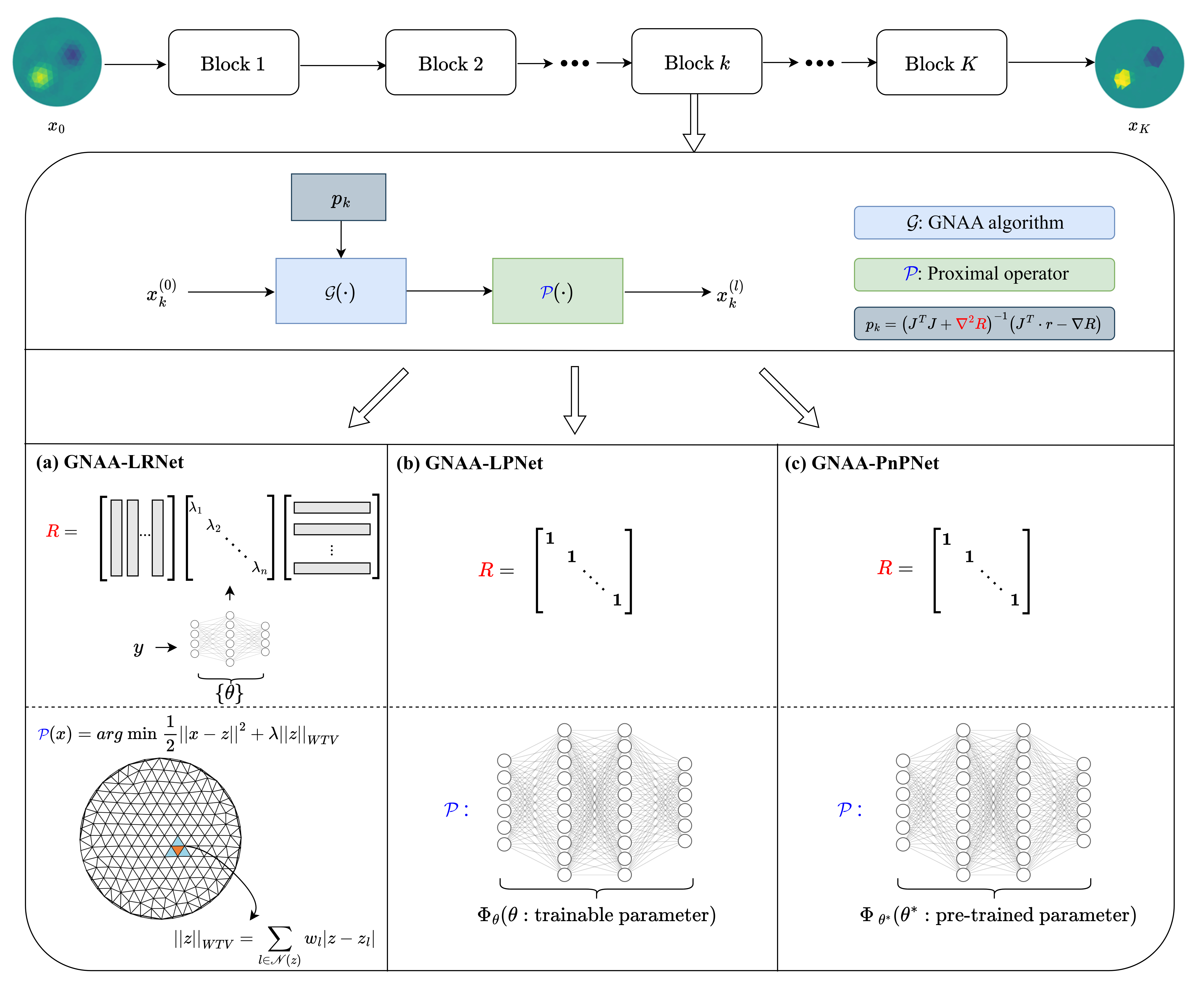
Figure 1: The three methods of GNAA-guided deep learning. (a) GNAA-LRNet: a deep neural network is used to learn the singular values of the smooth regularizer $R$, and a nonsmooth weighted total variation (WTV) is employed for the other regularizer $g$. (b) GNAA-LPNet: a Tikhonov regularizer is applied to $R$, and the proximal operator with regularizer $g$ is learned through a deep neural network. Particularly, the parameters of the network $\theta$ are trained alongside the whole network. (c) GNAA-PnPNet: also a Tikhonov regularization is employed for $R$, but differs in that the proximal operator with regularizer $g$ is directly replaced with a pre-trained deep denoiser. In this case, the parameters of the network $\theta^{*}$ are fixed.

Next we would like to consider applying the proximal Gauss-Newton method to the composite optimization, where our aim is to automatically learn the regularization parameters or even regularizer from training data. The proximal Gauss-Newton method starts from an initial value $x_{0}$, and performs the Gauss-Newton step and proximal step iteratively until convergence:

$$x^{\prime}_{k} =x_{k-1}-\beta H_{k-1}^{-1}\cdot\nabla f(x_{k-1})$$ (21a)

$$x_{k} =\mathcal{P}_{\lambda g}(x^{\prime}_{k}),$$ (21b)

where the proximal operator $\mathcal{P}_{\lambda g}(\cdot)$, dependent on the hyperparameter $\lambda$, is defined by

$$\mathcal{P}_{\lambda g}(x)=\underset{z}{\arg\min}\frac{1}{2}\|x-z\|^{2}+\lambda g\left(z\right),$$

and (21a) is the Gauss-Newton iteration. As discussed in Section 2.3, we introduce the Anderson acceleration to greatly accelerate convergence.

Finally, we propose three strategies to incorporate the GNAA algorithm into data-driven deep learning, which result in three flexible deep GNAA-Nets including GNAA-LRNet, GNAA-LPNet, and GNAA-PnPNet, as illustrated in Figure 1. GNAA of learned regularizer (GNAA-LRNet) method exploits a deep neural network to learn the regularizer of the GNAA method from training data. GNAA of learned proximity (GNAA-LPNet) method employs a deep neural network to learn the proximal operator, and GNAA of plug-and-play denoiser (GNAA-PnPNet) method directly replaces the proximal operator with any state-of-the-art deep denoiser. In the following subsections, we will discuss each approach in detail.

4.1 GNAA of learned regularizer

We are ready to present the explicit formulation of GNAA of a learned regularizer (GNAA-LRNet) model, which comprises two primary components. First, we will describe the derivation of the learned regularizer. Subsequently, we will discuss the explicit solution of a proximal operator problem with a weighted total variation (WTV).

4.1.1 Learned regularizer

To exploit the low-dimensional structure of $J$, we begin by computing its singular value decomposition, $J(x)=U\Sigma V^{T}$. Here, $U$ and $V$ are orthogonal matrices, and $\Sigma$ is a diagonal matrix with sequentially decreasing singular values. Using the columns of $V$ as a basis, we now construct the regularizer $R$ as follows:

$$R=V\Sigma_{\theta}V^{T}.$$ (22)

Here, the diagonal matrix $\Sigma_{\theta}$ will be determined through network learning. Referring to the general expression in (4) and choosing $R$ as described in (22), we derive the Gauss-Newton iteration:

$$x_{k+1}=x_{k}{\color[rgb]{0,0,0}+}\beta\tilde{p}_{k},$$ (23)

where

$$\tilde{p}_{k}=V\left(\Sigma^{2}+{\color[rgb]{0,0,0}\nabla^{2}\Sigma_{\theta}}\right)^{-1}V^{T}\left[J\left(x_{k}\right)^{T}\left({\color[rgb]{0,0,0}y}-F\left(x_{k}\right)\right){\color[rgb]{0,0,0}-}\alpha V\cdot\nabla\Sigma_{\theta}\cdot V^{T}\right].$$ (24)

As discussed in Section 2.3, the Gauss-Newton algorithm can be improved by using Anderson acceleration. To achieve this, in Algorithm 3 we can substitute $p_{k}$ in (8) with $\tilde{p}_{k}$ in (24).

4.1.2 Space-variant total variation

We adopt a class of space-variant total variation regularizers, known as the weighted total variation (WTV) [32], for the regularizer $g(x)$ in the proximal operator problem. This approach is tailored to mitigate specific shortcomings of the classical TV regularization, such as the staircasing and corner rounding effects.

Next we formulate the WTV on a two-dimensional triangular mesh. To clarify this concept, consider a planar domain $\Omega\subset\mathbb{R}^{2}$, represented by a triangulated mesh $(V,T,E)$, where $V\in\mathbb{R}^{n_{V}\times 2},V=\left\{v_{i}\right\}_{i=1}^{n_{V}}$ represents the set of vertices, $T\in\mathbb{R}^{n_{T}\times 3},T=\left\{\tau_{m}\right\}_{m=1}^{n_{T}}$ is the set of triangles and $E\in\mathbb{R}^{n_{E}\times 2},E=\left\{e_{j}\right\}_{j=1}^{n_{E}}$ is the set of edges. Then the WTV of the iteration $x_{k}$ reads as

$$\|x_{k}\|_{\text{WTV}}=\sum_{i=1}^{n_{T}}\sum_{l\in\mathcal{N}\left(\tau_{i}\right)}w_{l}\left|x_{k,i}-x_{k,l}\right|,\quad i=1,\ldots,n_{T}$$ (25)

where $\mathcal{N}\left(\tau_{i}\right)=\left\{\tau_{j}\in T:\tau_{j}\cap\tau_{i}\in V\right\}$ represents the set of the triangles $\tau_{j}\in T$ which share edges with the triangle $\tau_{i}$, and weight $w_{l}$ is associated to the triangle neighbor $\tau_{k}\in\mathcal{N}\left(\tau_{i}\right)$:

$$w_{l}=\frac{1}{\|\tau_{l}^{C}-\tau_{i}^{C}\|_{2}},$$ (26)

where $\tau_{k}^{C},\tau_{l}^{C}$ represent the centroid of the triangle $\tau_{k}$ and $\tau_{l}$, respectively. Note that when $w_{l}=1$, WTV simplifies to the classical TV regularizer. In the TV regularizer, each pixel $i=1,\ldots,N$ contributes equally to the overall regularization, rendering TV space-invariant. Therefore, TV fails to adequately represent diverse local image structures. In contrast, WTV introduces a space-variant weight $w_{i}$, allowing it to characterise local image features more effectively.

Finally, we provide a closed-form solution of the proximal operator problem with WTV regularizer, as proposed in Proposition 1 from [33].

Proposition 1.

Let $\tau$ be a generic triangle with $n$ the cardinality of $\mathcal{N}(\tau)$. Assuming $w_{k}>0$ be the weight defined in (26) and associated to $\tau_{k}\in\mathcal{N}(\tau)$, the values $x_{k}$ on $\tau_{k}\in\mathcal{N}(\tau)$ be sorted as $x_{k,1}\leq x_{k,2}\leq\ldots\leq x_{k,n}$. The minimizer of problem

$$\mathcal{P}_{\text{WTV}}(x_{k})=\underset{z}{\arg\min}\frac{1}{2}\|x_{k}-z\|^{2}+\lambda\|z\|_{\text{WTV}},$$

is given by

$$z^{*}=\operatorname{median}\left\{x_{k,1},\ldots,x_{k,n},x_{k,1}+\frac{1}{2}W_{1},\ldots,x_{k,n}+\frac{1}{2}W_{n}\right\},$$

with

$$W_{j}=-\sum_{k=1}^{j}w_{k}+\sum_{k=j+1}^{n}w_{k},\quad j=1,\cdots,n.$$

4.1.3 GNAA-LRNet

Now we summarize the complete procedure of GNAA of a learned regularizer (GNAA-LRNet) algorithm, by using the methods discussed in Sections 4.1.1 and 4.1.2. Specifically, starting from an initial $x_{0}$, the algorithm performs the following steps:

$$x^{\prime}_{k} =\mathcal{G}(x_{k-1};{\color[rgb]{0,0,0}y},m,\{{\color[rgb]{0,0,0}\tilde{p}_{i}}\}_{i=k-m+1}^{k})$$ (27a)

$$x_{k} =\mathcal{P}_{\text{WTV}}(x^{\prime}_{k}),$$ (27b)

where (27a) is specified in Algorithm 3 with the substitution of $p_{k}$ by $\tilde{p}_{k}$, and the closed-form solution of  (27b) is provided by Proposition 1.

4.2 GNAA of learned proximity

We let the smooth regularization $R(x)$ in problem (20) to be a Tikhonov regularization, which is the most popular regularization for nonlinear least squares problems. A common choice for $R(x)$ reads as

$$R(x)=\|L(x-x_{0})\|_{2}^{2},$$

where $x_{0}$ is a prior estimate of $x$, and $L$ is an appropriately chosen regularizing matrix, such as discrete differential operator, positive diagonal matrix, and simply the identity matrix. We then assume $g(x)$ to be any regularization function, we can obtain

$$f_{g}(x)=\frac{1}{2}\|y-F(x)\|_{2}^{2}+\alpha\|L(x-x_{0})\|_{2}^{2}+\lambda g(x).$$ (28)

In this setting, the gradient and the approximated Hessian matrix of the objective function in (28) are given as follows:

$$\nabla f(x_{k}) =J\left(x_{k}\right)^{T}\left({\color[rgb]{0,0,0}F\left(x_{k}\right)-y}\right)+{\color[rgb]{0,0,0}2}\alpha L^{T}L\left(x_{k}-x_{0}\right)$$

$$H_{k} =J\left(x_{k}\right)^{T}J\left(x_{k}\right)+{\color[rgb]{0,0,0}2}\alpha L^{T}L.$$

Next we follow  [7] to use parameterized neural networks $\Phi_{\theta}$ to replace the proximal operators $\mathcal{P}_{\lambda g}$. This gives the GNAA of the learned proximal operator (GNAA-LPNet) algorithm. Specifically, within each block, each inner iteration starting from an initial $x_{0}$ performs the following steps:

$$x^{\prime}_{k} =\mathcal{G}(x_{k-1};{\color[rgb]{0,0,0}y},m,\{{\color[rgb]{0,0,0}p_{i}}\}_{i=k-m+1}^{k})$$ (29a)

$$x_{k} =\Phi_{\theta}(x^{\prime}_{k}).$$ (29b)

Note that the parameterized neural networks with independent weights in different block, i.e. $\Phi_{\theta_{k}}$ has trainable parameters $\theta_{k}$ in the kth block, is another commonly used strategy [34]. In our numerical experiments we have tested this setting, and found no significant difference between the performances of sharing and independent weights. As such, we focus on sharing weights in this work.

4.3 GNAA of plug-and-play denoiser

The incorporation of the GNAA and pluy-and-play is a bit different. Instead of replacing the regularizing proximal operator with a learned deep neural network, we consider applying a deep denoiser in the proximal step. Replacing the proximal operator with a deep denoiser results in the GNAA of plug-and-play deep denoiser (GNAA-PnPNet) method. Technically speaking, a key difference between GNN-LPNet and GNAA-PnPNet is that we use a pre-trained deep denoiser so the parameters of the deep denoiser are fixed, while the paramters of the proximal learning network are trainable. Once the deep denoiser $\Phi_{\theta^{*}}$ is well trained, GNAA-PnPNet performs the following iterates until convergence:

$${x}^{\prime}_{k} =\mathcal{G}(x_{k-1};{\color[rgb]{0,0,0}y},m,\{{\color[rgb]{0,0,0}p_{i}}\}_{i=k-m+1}^{k})$$ (30a)

$$x_{k} =\Phi_{\theta^{*}}({x}^{\prime}_{k}).$$ (30b)

In our numerical experiments, we process the simulated data from the finite element method as graph data. For computational convenience, we utilize a graph U-Net (g-U-Net) [35] as the plug-and-play denoiser. It is worth noting that classical denoisers such as NLM and BM3D [36], as well as data-driven CNN-based denoisers such as DnCNN [37] and residual U-net [38] can also be utilized after converting the graph data to pixel data.

5 Numerical experiments

In this section, we evaluate the performances of the GNAA-Nets discussed so far, namely GNAA-LRNet, GNAA-LPNet, and GNAA-PnPNet in comparison with EITGN-NET [39] and GNAA as well as the regularized GN (RGN) method [40]. As an example, we will consider the electrical impedance tomography (EIT) inverse problem.

5.1 EIT inverse problems

Assume that $L$ different electrical currents are injected into the boundary of objects ($\partial\Omega$) and the resulting electrical potential should satisfy the following $L$ governing equations with different boundary conditions:

$$\left\{\begin{array}[]{ll}\nabla\cdot(\sigma\nabla u)=0&\text{ in }\Omega,\\ u+z_{l}\sigma\frac{\partial u}{\partial n}=v_{l}&\text{ on }E_{l},l=1,\ldots,L,\\ \int_{E_{l}}\sigma\frac{\partial u}{\partial n}\mathrm{~{}d}s=I_{l}&\text{ on }\Gamma,\\ \sigma\frac{\partial u}{\partial n}=0&\text{ on }\tilde{\Gamma},\end{array}\right.$$ (35)

where $\Gamma(\tilde{\Gamma})$ is the boundary of object $\partial\Omega$ with (without) electrodes, $v_{l}$ is the voltage measured by $l$-th electrode $E_{l}$ when the currents $I_{l}$ are applied, $z_{l}$ is the contact impedance, $u$ is the electric potential in the interior of the object $\Omega$, and $n$ is the normal to the object surface. Typically, the solution to the forward EIT problem involves applying the finite element method [41] to solve the boundary problem (35).

Besides, we confine the conductivities $\sigma$ to a finite-dimensional space comprising piecewise polynomials defined on a discretized domain $\Omega$, consisting of $n_{T}$ triangles. Each polynomial segment maintains a constant value for $\sigma$ within its respective triangle.

Mathematically, the EIT inverse problem involves recovering the conductivity $\sigma$ within the domain $\Omega$ based on the measurements $v$ and the nonlinear forward operator $F(\sigma)$. The purpose of the so-called absolute imaging problem is to estimate the conductivity $\sigma$ by solving the following function:

$$\hat{\sigma}\in\mathop{\arg\min}\limits_{\sigma}\frac{1}{2}\|v-F(\sigma)\|_{2}^{2}+\alpha R(\sigma)+\lambda g(\sigma),$$

where $\frac{1}{2}\|v-F(\sigma)\|_{2}^{2}$ is the data fidelity term, $R$ is a convex and smooth regularizer, $g$ is a potential nonconvex and non-smooth regularizer, and $\alpha,\lambda$ are trade-off parameters.

5.2 Simulations and Implementation Details

Within our simulated datasets, each sample represents the ground-truth conductivity denoted as $\sigma^{*}$. These samples are composed of anomalies situated within a circular tank of unitary radius. The number of anomalies in each sample ranges randomly from 1 to 4. Each anomaly is characterized by its position, which is randomly distributed within the tank, as well as its radius (ranging from 0.15 to 0.25) and magnitude (ranging from 0.2 to 2), both assigned randomly. The circular tank is divided into a mesh grid consisting of 660 triangles. Along the circular boundary, 16 electrodes are evenly spaced. The background conductivity is assumed to be homogeneous with a value of $\sigma_{0}=1.0\ \Omega m^{-1}$, and it is assumed that each anomaly is composed of a similar material. The voltage $u$ corresponding to the conductivity distribution is calculated using the Finite Element Method to simulate the real voltage measurement process. Additionally, it is assumed that this simulation process is noise-free. All the examples and measurements are simulated via pyEIT [42], a python based tools for electrical impedance tomography.

In the training, we utilized a set of 250 randomly generated examples. Out of these, 200 examples were allocated for training the models, while the remaining 50 examples were reserved to evaluate the performance of the proposed methods.

In particular, for the plug-and-play strategy, we incorporate the GU-Net-Denoiser mentioned earlier to provide prior information during training. Further details regarding its implementations can be found in B.

In our implementations, the learning rate is set to $0.01$. We find that 30 epochs were sufficiently decreased the total loss function. The training is implemented on a PC with Intel i7 CPU and 16-GB RAM with Pytorch, and Adam has been used for optimization.

5.3 Metrics

The evaluations are performed using both qualitative and quantitative assessments. Qualitatively, artifacts are visually inspected, while quantitatively, regular metrics such as mean-square error (MSE) and structural similarity (SSIM) are calculated.

Dynamic range, another vital metric used in this study to evaluate the quality of the reconstructed conductivity distribution, is defined as

$$DR=\frac{\max\sigma-\min\sigma}{\max\sigma^{*}-\min\sigma^{*}}\times 100\%,$$

a DR value closer to 100 signifies optimal reconstruction quality.

Besides, we use the electrical impedance tomography evaluation index (EIEI) to evaluate the homogeneity of anomalies in EIT. We denote $n_{1}$, $n_{2}$, and $n_{3}$ as the number of triangles occupied by backgrounds, artifacts and anomalies, respectively. The associated conductivity values are denoted by $\sigma^{(1)}$, $\sigma^{(2)}$, and $\sigma^{(3)}$. We adopt the clustering method to estimate the variances of these three clusters, as described in [39]:

$$\delta_{j}=\sum_{i=1}^{n_{j}}|\sigma_{i}^{(j)}-\bar{\sigma}^{(j)}|/n_{j},\ \ \ j=1,2,3.$$

where $\sigma_{i}^{(j)}$ represents the conductivity value associated with the $i_{th}$ triangle with a value of $\sigma^{(j)}$, and $\bar{\sigma}^{(j)}$ denotes the average conductivity value. The EIEI metric is then defined as follows:

$$EIEI=w_{1}T_{1}+w_{2}T_{2},$$

where $T_{1}=1-n_{2}/n_{T}$ is the number of artifact triangles and $T_{2}=1-(\delta_{1}n_{1}/n_{T}+\delta_{3}n_{3}/n_{T})$ iss the number of backgrounds and anomalies triangles. The weighting values $w_{1}$ and $w_{2}$ represent the certainty levels of $T_{1}$ and $T_{2}$, and are evaluated as

$$w_{1}=\sum_{i=1}^{n_{2}}\sigma_{i}^{(2)}/n_{2},\ \ w_{2}=\left(\sum_{i=1}^{n_{1}}\sigma_{i}^{(1)}+\sum_{i=1}^{n_{3}}\sigma_{i}^{(3)}\right)/(n_{1}+n_{3}).$$

This metric provides qualitative insight via an EIEI map, where yellow indicates artifacts, red indicates anomalies, and blue represents background.

These metrics are specifically designed to evaluate the effectiveness of EIT reconstructions. For detailed information on the implementation of these metrics, see [39]. In all experiments pertaining to GNAA, we manually fine-tuned the regularization parameter $\alpha$ to ensure the attainment of optimal performance in terms of MSE values.

5.4 Results and discussion

5.4.1 Benefit of AA scheme

Initially, we conducted experiments to validate the efficacy of the AA scheme. The results, as presented in Table 1, showcase the varied performance of Anderson acceleration under four different strategic frameworks. In particular, with the application of Anderson acceleration, both MSE and SSIM show considerable enhancements compared to scenarios without acceleration. For instance, under the learned-proximal strategy, Anderson acceleration leds to a 39.7$\%$ reduction in MSE and a 6.7$\%$ increase in SSIM, which demonstrates that the AA scheme significantly enhances the experimental outcomes in different frameworks.

Table 1: The performance of the reconstructions for EIT in terms of MSE, SSIM, and DR metrics by ablation study within 30 iterations, where ✘ indicates the algorithm without Anderson acceleration and ✔ indicates the algorithm with Anderson acceleration.

• Method	GN with AA	MSE	SSIM	DR
  GN	✘	4.72$\times 10^{-3}$	0.86	102
  GNAA	✔	3.90$\times 10^{-3}$	0.88	124
  GN-LR	✘	4.39$\times 10^{-3}$	0.90	102
  GNAA-LRNet	✔	2.87$\times 10^{-3}$	0.94	115
  GN-PnP	✘	3.30$\times 10^{-3}$	0.95	112
  GNAA-PnPNet	✔	2.46$\times 10^{-3}$	0.96	119
  GN-LP	✘	3.60$\times 10^{-3}$	0.90	112
  GNAA-LPNet	✔	2.17$\times 10^{-3}$	0.96	101

Figure 2 demonstrates the convergence of the iterative GNAA schemes with various Anderson depth $m$ towards the optimal solution $\sigma^{*}$ in four representative test cases. In particular, the plots report the relative errors $e_{k}$, in terms of the number $k$ of iterations

$$e_{k}=\frac{\|\sigma_{k}-\sigma^{*}\|_{2}}{\|\sigma^{*}\|_{2}}.$$ (36)

The findings depicted in Figure 2 highlight the direct impact of different values of $m$ on the reconstruction results. Specifically, as $m$ increases, the experimental performance shows a notable improvement. However, it is observed that once $m$ reaches or surpasses 5, the iterations converge, and further increases in $m$ do not yield substantial enhancements.

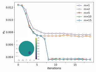
(a) 1 anomaly

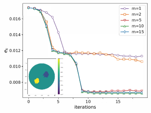
(b) 2 anomalies

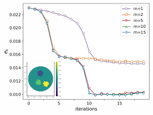
(c) 3 anomalies

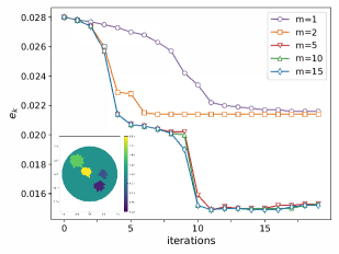
(d) 4 anomalies

Figure 2: Relative error $e_{k}$ between $\sigma^{GT}$ and the approximated solutions obtained by the algorithm GNAA with various Anderson depth $m$ for different test cases.

5.4.2 Performance comparisons

We evaluate the performance of three proposed proximal Gauss-Newton-Anderson-type frameworks, namely GNAA-LRNet, GNAA-LPNet, and GNAA-PnPNet, by comparing them with the Regularized Gauss-Newton method (RGN) which uses the pyEIT library, the original GNAA (Algorithm 3) method, and the EITGN-NET method mentioned above.

Table 2 presents a comparison of performance based on the averaged MSE, SSIM, DR metrics and time costs across a set of 50 test cases. It is evident that three GNAA-Nets, i.e. GNAA-LPNet, GNAA-LRNet, and GNAA-PnPNet, have made considerable improvements compared to the state-of-the-arts method (EITGN-NET) as well as the classical methods (GNAA, RGN) across all metrics. To be more specific, in terms of MSE, GNAA has reduced $17.4\%$ compared to traditional RGN, while GNAA-LPNet, GNAA-LRNet and GNAA-PnPNet have reduced $54.0\%$, $39.2\%$ and $47.9\%$ respectively, which not only demonstrates the effectiveness of Anderson acceleration, but also indicates the superior performance of these three learning-based frameworks.

Table 2: Performance evaluation of GNAA-LPNet, GNAA-LRNet, GNAA-PnPNet, GNAA, EITGN-NET and RGN in terms of MSE, SSIM, DR Metrics, and time costs for inference.

	GNAA-LPNet	GNAA-LRNet	GNAA-PnPNet	EITGN-NET	GNAA	RGN
MSE	2.17$\boldsymbol{\times 10^{-3}}$	2.87$\times 10^{-3}$	2.46$\times 10^{-3}$	2.94$\times 10^{-3}$	3.90$\times 10^{-3}$	4.72$\times 10^{-3}$
SSIM	0.96	0.94	0.96	0.93	0.88	0.86
DR	101	115	119	115	124	102
Time (sec)	18.63	34.53	10.60	21.15	10.13	10.29

The visual comparison can be found in Figure 3. The visual results clearly demonstrate that GNAA-LPNet, GNAA-LRNet, and GNAA-PnPNet generate reconstructions with fewer artifacts and higher fidelity compared to GNAA and RGN. Furthermore, these three frameworks effectively enhance the differentiation among anomalies. Notably, among these three frameworks, GNAA-LPNet outperforms the others with minimal artifacts and the highest EIEI values.

   a

   EIEI:

   c

   EIEI:

   e

   EIEI:

   e

   EIEI:

(a) GT

   2.15

   2.20

   2.10

   1.97

(b) GNAA-
  LPNet

   2.14

   1.95

   1.92

   1.95

(c) GNAA-
  LRNet

   2.14

   2.03

   2.07

   2.04

(d) GNAA-
  PnPNet

   2.13

   2.05

   1.95

   1.82

(e) EITGN-NET

   1.99

   1.84

   1.81

   1.73

(f) GNAA

   1.84

   1.73

   1.63

   1.59

(g) RGN

Figure 3: Visual reconstruction performance comparisons between GNAA-LPNet, GNAA-LRNet, GNAA-PnPNet, EITGN-NET, original GNAA and RGN with varying numbers of anomalies are shown in the top rows, EIEI values are reported for each case with the associated structure maps on the bottom.

5.4.3 Sensitivity analysis for initial values

For non-convex problems, both traditional iterative optimization methods and the GNAA approach are highly sensitive to the selection of initial points. Therefore, to assess the performance of our GNAA algorithm, we conducted extensive validation experiments using three different deep learning architectures and varying initial points. The initial points considered were $x_{GN}$ (obtained after 8 iterations of Gauss-Newton method), $\mathbf{1}_{660\times 660}$ (a matrix filled with ones), and randomly selected initial points generated from the random distribution.

In the error plots depicted in Figure 4, we observe the variation of the error defined in (36) over iterations and time for the methods of RGN, GNAA, GNAA-LPNet, GNAA-LRNet, and GNAA-PnPNet, with the consideration of both types of initial points for the case with 1 anomaly (as shown in Figure 2). It is obvious that, the proposed GNAA-PnPNet exhibits consistently fast convergence and superior performance across different initial points, particularly in the case of $\mathbf{1}_{660\times 660}$. GNAA-LRNet also demonstrates favorable performance across various initial points, although it needs a higher computational cost. In contrast, GNAA-LPNet tends to be more heavily dependent on the choice of initial points. Under appropriate initial point conditions, GNAA-LPNet can achieve the best performance, as illustrated in Figure 4(a). Additionally, when consider diverse initial conditions, GNAA exhibits faster convergence compared to the traditional RGN method.

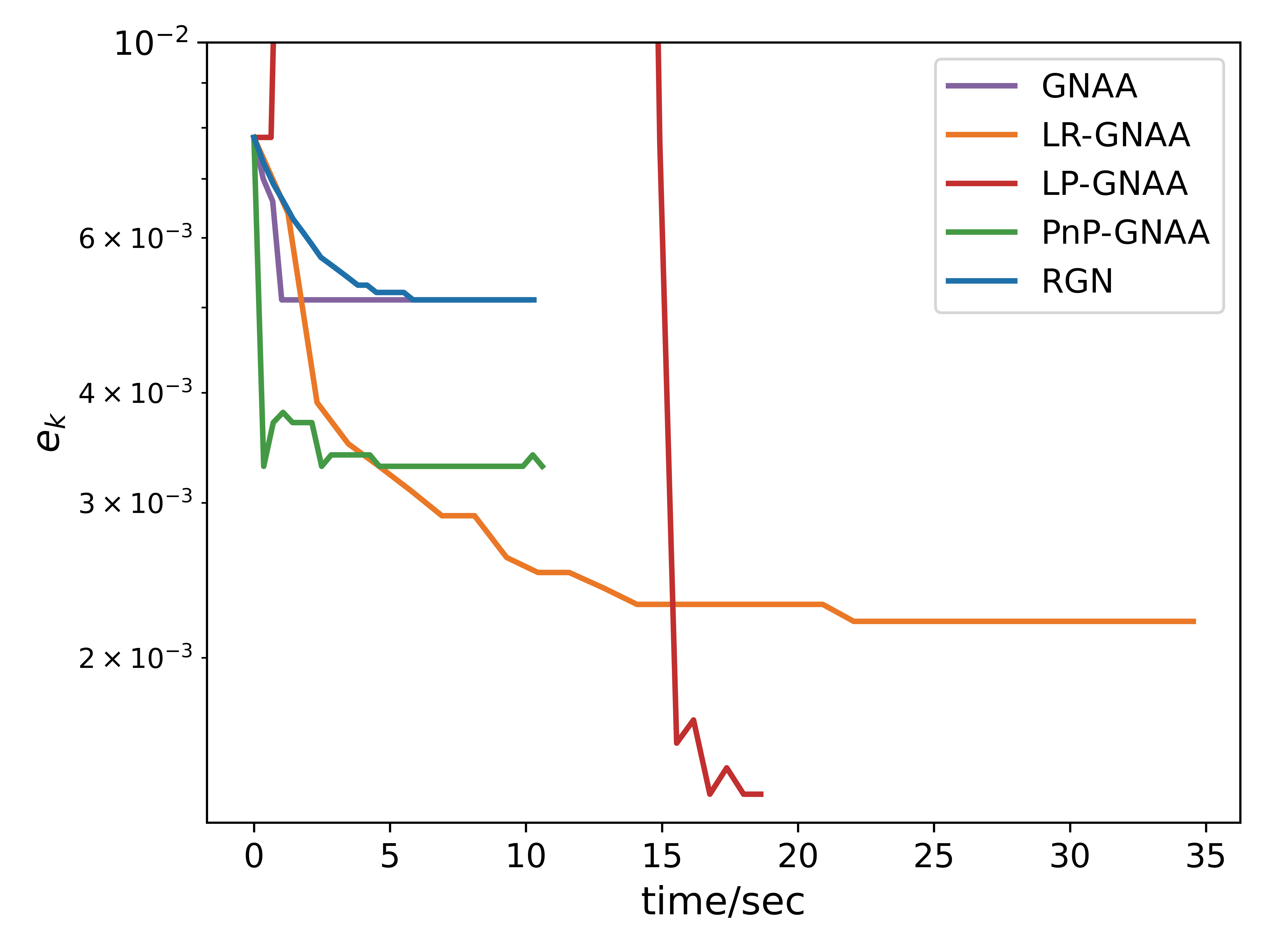
(a) $x_{0}=x_{GN}$

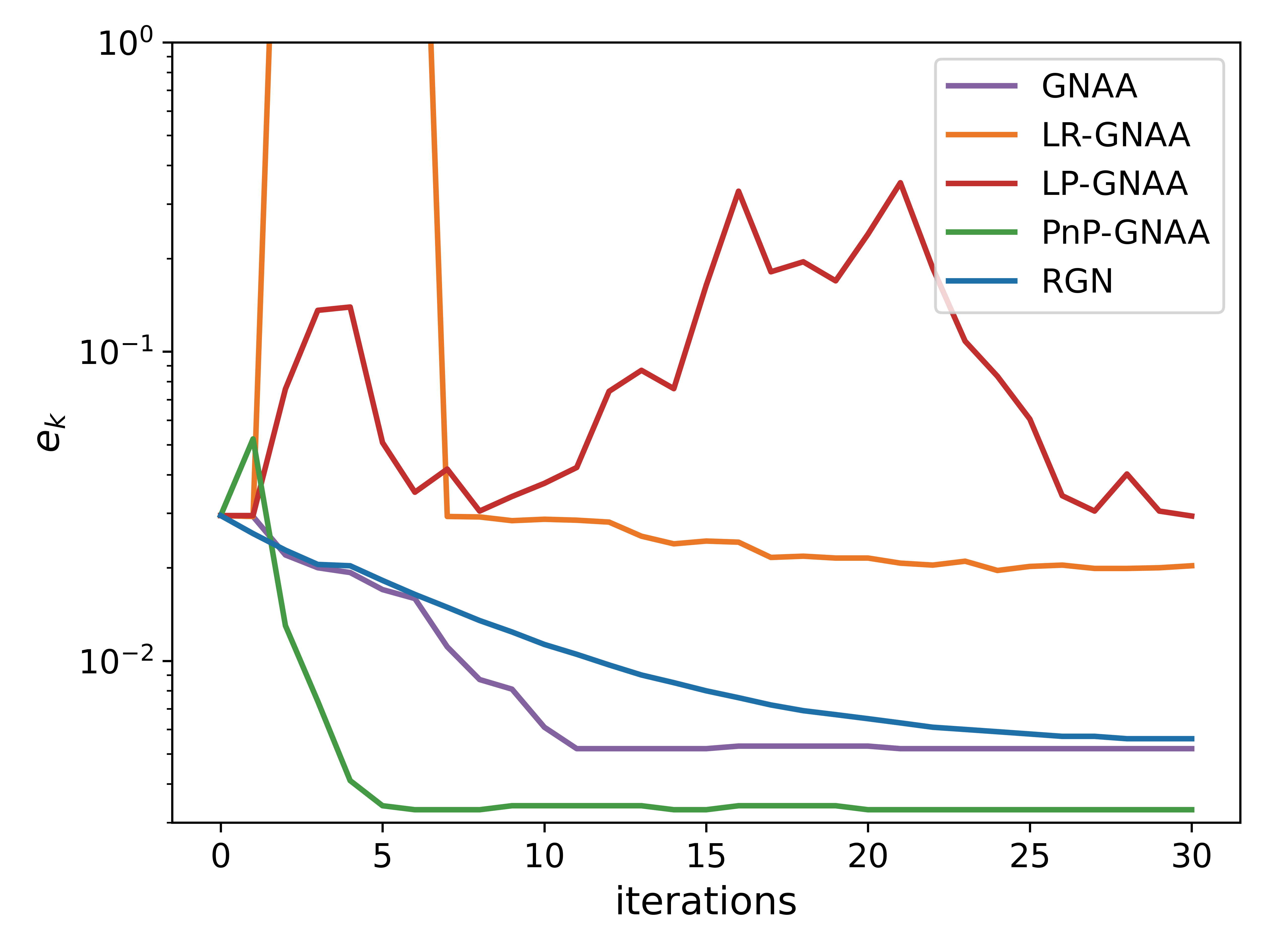
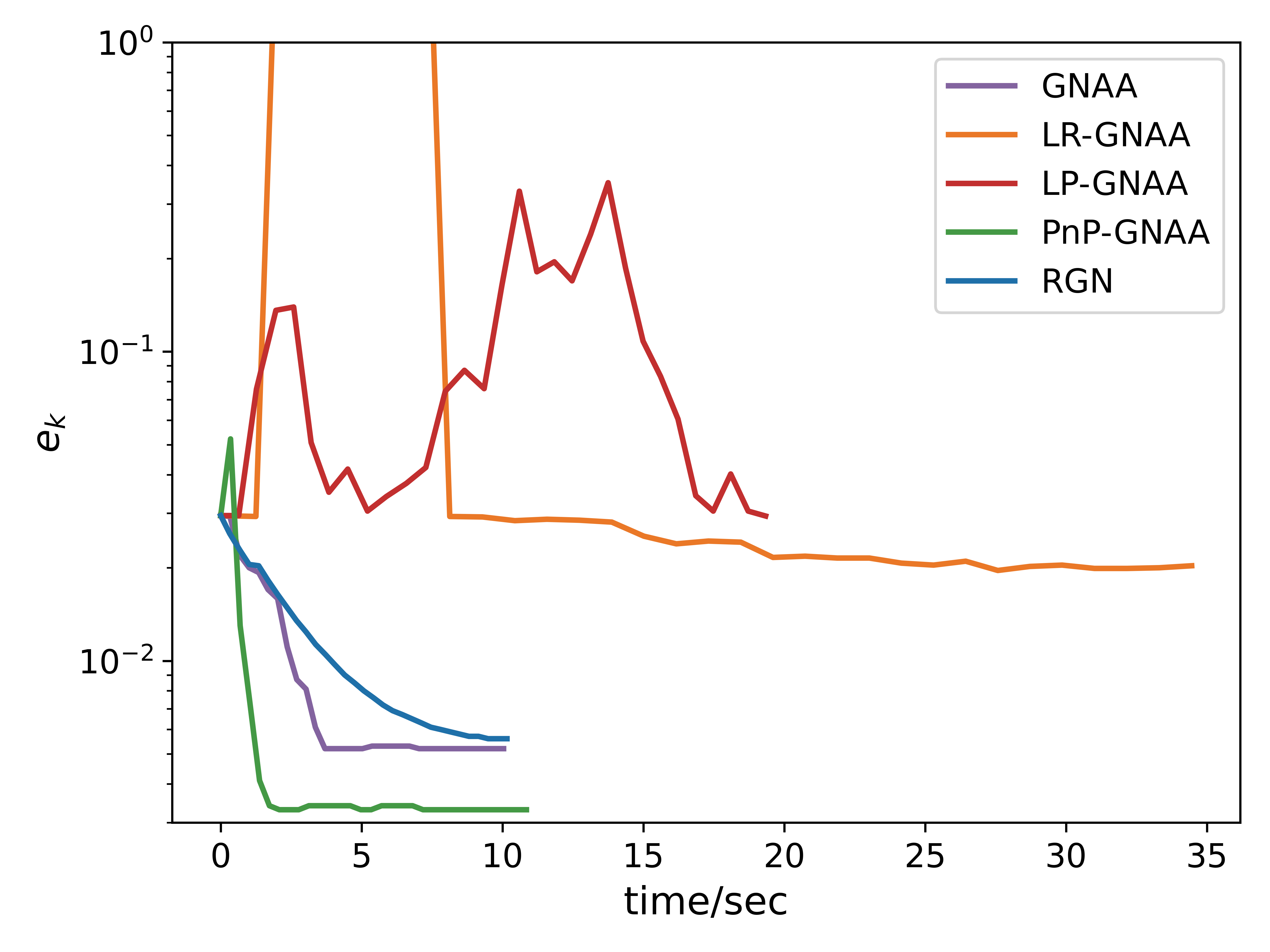
(b) $x_{0}=\mathbf{1}_{660\times 660}$

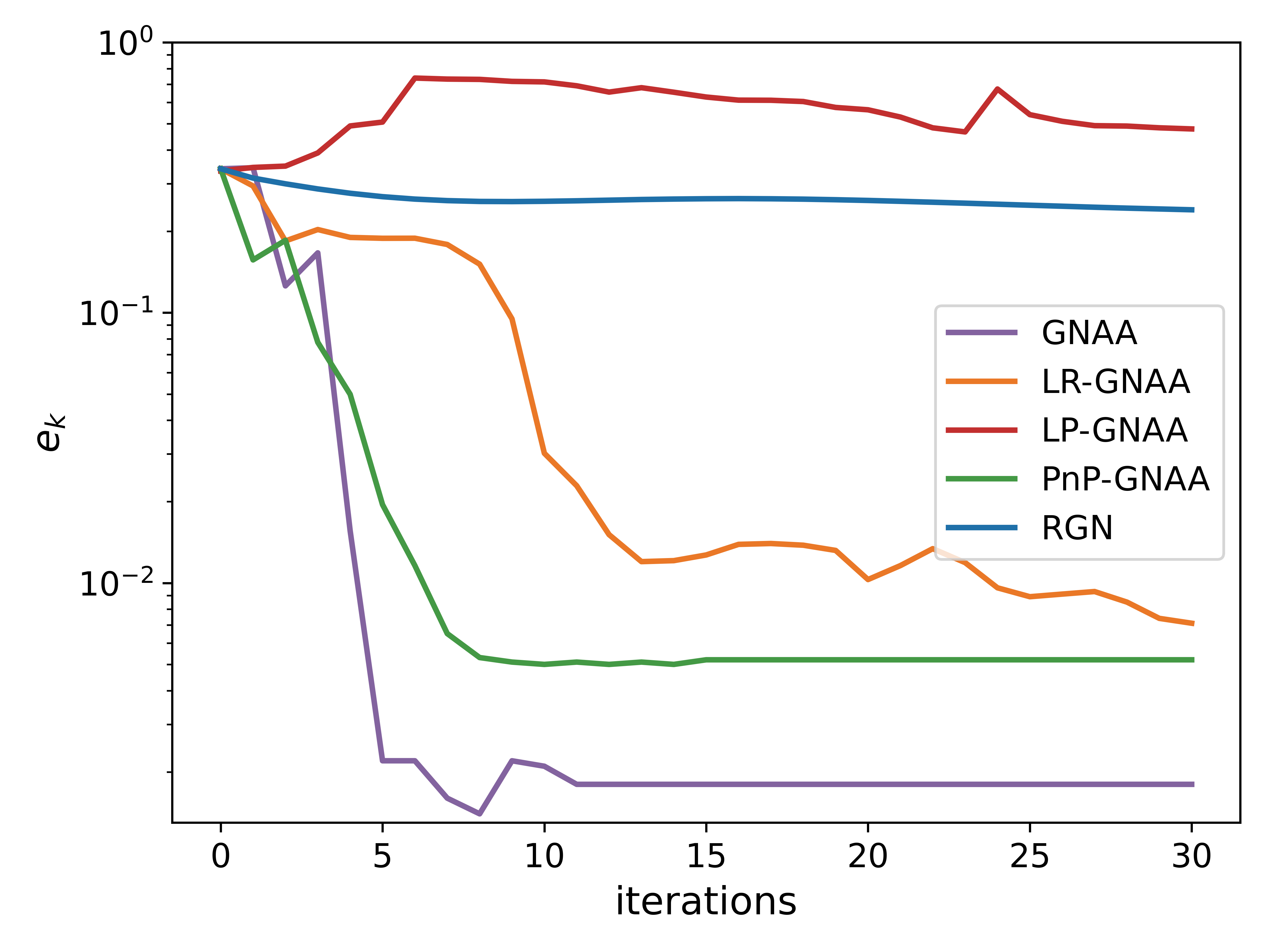
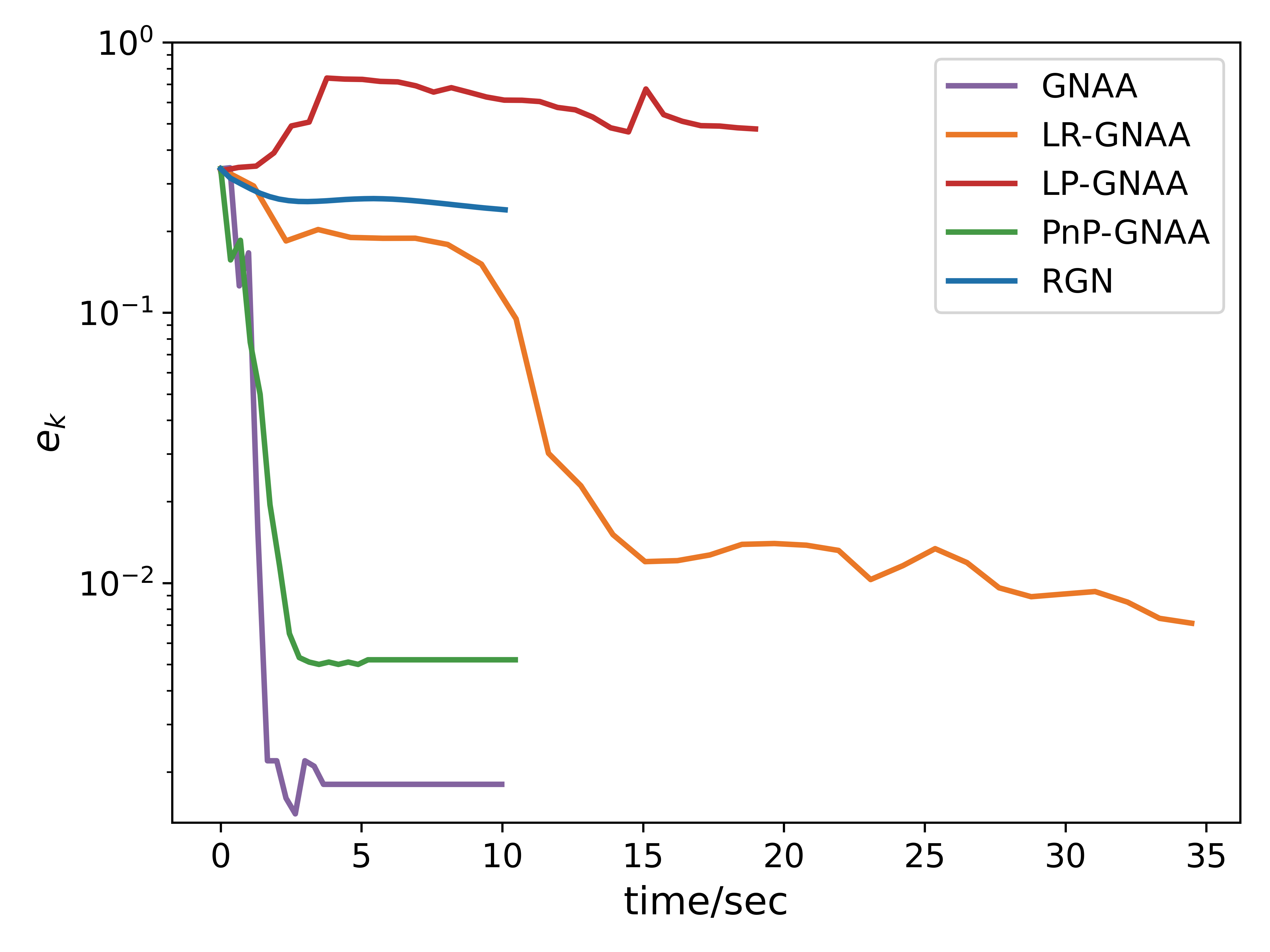
(c) $x_{0}=$random value

Figure 4: Under different initial conditions, the relative error variations and temporal changes of various proximal GNAA types methods are examined using case with 1 anomaly as test scenario within 30 iterations.

6 Conclusion

We developed three GNAA-guided deep learning methods, grounded on the provably convergent Gauss-Newton Anderson acceleration (GNAA), to solve nonlinear inverse problems. Our methods exploit the automatic determination of singular values of the regularization matrix, the data-driven regularizer, and the incorporation of the deep denoiser technique. They draw benefits from both the theoretical constraints of physical principles and the prior knowledge of training data, inverse problems are then successfully solved, including those encountered in electrical impedance tomography (EIT). Numerical experiments demonstrate the effectiveness and rapid convergence rate of the proposed method quantitatively and visually.

Appendix A Proof of Lemma 3.2.1

For all $x,y\in\mathbb{R}^{n}$, we can prove that

$$\begin{array}[]{ll}\|M(x)-M(y)\|&=\|J^{T}(x)J(x)+\alpha\nabla^{2}R(x)-J^{T}(y)J(y)-\alpha\nabla^{2}R(y)\|\\ &\leq\|J^{T}(x)J(x)-J^{T}(y)J(y)\|+\alpha\|\nabla^{2}R(x)-\nabla^{2}R(y)\|\|\\ &\leq(2\varepsilon\beta+\alpha\eta)\|x-y\|.\end{array}$$

Similarly, for $H(x)$ and $M(x)$ there are same conclusions

$$\begin{array}[]{ll}\|H(x)-H(y)\|&=\|H(x)[M(y)-M(x)]H(y)\|\leq w^{2}(2\varepsilon\beta+\alpha\eta)\|x-y\|,\\ \end{array}$$

and also

$$\begin{array}[]{ll}\|S(x)-S(y)\|&=\|\nabla^{2}f(x)-M(x)-\nabla^{2}f(y)+M(y)\|\leq(2\varepsilon\beta+\alpha\eta+\gamma)\|x-y\|.\\ \end{array}$$

Expanding $\nabla f(x^{*})$ at $x_{l}$ gives

$$0=\nabla f(x^{*})=\nabla f(x_{l})-\nabla^{2}f(x_{l})e_{l}^{*}+O(\|e_{l}^{*}\|^{2}).$$

Multiplying both sides of the above equation by $H_{l}=H(x_{l})=[M(x_{l})]^{-1}$ simultaneously gives

$$\begin{array}[]{ll}0&=[J^{T}(x_{l})J(x_{l})+\alpha\nabla^{2}R(x_{l})]^{-1}\cdot(J(x_{l})r(x_{l})+\alpha\nabla^{2}R(x_{l}))-H_{l}(H_{l}^{-1}+S_{l})e_{l}^{*}+O(\|e_{l}^{*}\|^{2})\\ \end{array}$$

which is equivalent to

$$0=-e_{l+1}^{*}-H_{l}S_{l}e_{l}^{*}+O(\|e_{l}^{*}\|^{2}),$$

thus, we have

$$\begin{array}[]{ll}e_{l+1}^{*}&=-H_{l}S_{l}e_{l}^{*}+O(\|e_{l}^{*}\|^{2})\\ &=-H(x^{*})S(x^{*})e_{l}^{*}-H_{l}(S_{l}-S(x^{*}))e_{l}^{*}-(H_{l}-H(x^{*}))S(x^{*})e_{l}^{*}+O(\|e_{l}^{*}\|^{2}),\end{array}$$

therefore,

$$\|e_{l+1}^{*}\|\leq\|H(x^{*})S(x^{*})\|\cdot\|e_{l}^{*}\|+O(\|e_{l}^{*}\|^{2}).$$

The next iteration of GNAA(m) can be represented by

$$\begin{array}[]{ll}x_{k+1}&=x_{k}+w_{k+1}-\sum_{j=k-m+1}^{k}[(x_{j}-x_{j-1})+(w_{j+1}-w_{j})]\gamma_{j}\end{array}$$

which can be transfromed into

$$x_{k+1}=(x_{k}+w_{k+1})(1-\gamma_{1})+\sum_{j=k-m+1}^{k-1}(x_{j}+w_{j+1})(\gamma_{k-j}-\gamma_{k-j+1})+(x_{k-m}+w_{k-m+1})\gamma_{m},$$

we can rewrite $x^{*}=x^{*}[(1-\gamma_{1})+(\gamma_{1}-\gamma_{2})+\cdots+(\gamma_{m-1}-\gamma_{m})+\gamma_{m}]$, and

$$\begin{array}[]{ll}x_{k+1}-x^{*}&=(x_{k}+w_{k+1}-x^{*})(1-\gamma_{1})+\sum_{j=k-m+1}^{k-1}(x_{j}+w_{j+1}-x^{*})(\gamma_{k-j}-\gamma_{k-j+1})\\ &\quad+(x_{k-m}+w_{k-m+1}-x^{*})\gamma_{m},\end{array}$$

then we have

$$\begin{array}[]{ll}\|e_{k+1}^{*}\|&\leq\|H(x^{*})S(x^{*})\|\cdot\bar{\gamma}_{k}\cdot\sum_{j=k-m}^{k}\|e_{j}^{*}\|+O(\|e_{j}^{*}\|^{2})\\ &\leq w\cdot L\cdot\bar{\gamma}_{k}\cdot\sum_{j=k-m}^{k}\big{(}\|e_{j}^{*}\|+O(\|e_{j}^{*}\|^{2})\big{)},\end{array}$$

where $\bar{\gamma}_{k}=\max\{2\|\gamma_{k}\|_{\infty},1+\|\gamma_{k}\|_{\infty}\}$.

Appendix B Training strategy of the GU-Net-Denoiser

The GU-Net-Denoiser is trained on the training dataset with an initial set of random weights. Through the training process, these weights are iteratively optimized, leading to the derivation of an optimal set of weights. This optimal set of weights is then employed in the GNAA-PnPNet method for improved performance.

The pre-trained GU-Net-Denoiser has a network depth $M=12$ (number of layers) for encoder and decoder, and the down-sampling (up-sampling) factor 0.6. More details about the network structure, see [35].

The training dataset comprises 18,000 samples, denoted as $(x^{GT},\hat{x}^{j})$, where each sample consists of 3,000 distinct conductivity configurations. For each configuration, there are six reconstructions available: the ground-truth $x^{GT}$ itself (corresponding to $j=0$), as well as $\hat{x}^{j}$ for $j=1,\cdots,5$, representing reconstructions with increasing levels of accuracy or decreasing levels of noise. The reconstructions $\hat{x}^{j},j=1,\cdots,5$ are obtained by applying the LM algorithm for 4, 5, 6, 7, and 8 iterations, respectively, starting from the corresponding collected voltages $v$.

The training process is about to minimize the following loss function over the training set of size $n_{S}$ during each epoch $k$:

$$\begin{gathered}\theta_{k}^{*}\leftarrow\operatorname{argmin}_{\theta_{k}}\frac{1}{n_{S}}\mathcal{L}\left(\theta_{k}\right),\\ \text{ where }\mathcal{L}\left(\theta_{k}\right)=(1-\gamma)\sum_{i=1}^{n_{S}}\sum_{j=0}^{5}\left\|\mathcal{G}\left(\hat{x}_{i}^{j};\theta_{k}\right)-x_{i}^{GT}\right\|_{2}^{2}+\gamma\sum_{i=1}^{n_{S}}\sum_{j=0}^{5}\left\|\mathcal{G}\left(\hat{x}_{i}^{j};\theta_{k}\right)-x_{i}^{GT}\right\|_{1},\end{gathered}$$ (38)

with $\gamma\in(0,1)$, and $\mathcal{G}(\cdot;\theta_{k})$ being the deep GU-Net denoiser. In particular, the training phase for the reported examples used $\gamma=0.2$. After the completion of 150 training epochs, we observed a substantial reduction in the overall loss function (38). This indicated that the model had converged effectively. Consequently, we determined that the weights $\theta_{150}$ obtained at the $150th$ epoch would serve as the initial parameters for the GU-Net-Denoiser during the inference phase.

For training, we utilized a learning rate of $2.5\times 10^{-3}$ and employed the standard Adam optimizer. The network implementation was done by using PyTorch and PyTorch Geometric [43] libraries. The experiments were conducted on a PC with an Intel i7 CPU, 16 GB of RAM, and an NVIDIA 3060 GPU, ensuring efficient and reliable computation.

References

References

- [1] Ge Wang, Jong Chul Ye, and Bruno De Man. Deep learning for tomographic image reconstruction. Nature Machine Intelligence, 2(12):737–748, 2020.
- [2] William RB Lionheart. EIT reconstruction algorithms: pitfalls, challenges and recent developments. Physiological measurement, 25(1):125, 2004.
- [3] Richard Bayford, Rosalind Sadleir, and Inéz Frerichs. Advances in electrical impedance tomography and bioimpedance including applications in COVID-19 diagnosis and treatment. Physiol. Meas., 43(2):020401, 2022.
- [4] George Em Karniadakis, Ioannis G Kevrekidis, Lu Lu, Paris Perdikaris, Sifan Wang, and Liu Yang. Physics-informed machine learning. Nature Reviews Physics, 3(6):422–440, 2021.
- [5] Kaixuan Wei, Angelica Aviles-Rivero, Jingwei Liang, Ying Fu, Hua Huang, and Carola-Bibiane Schönlieb. TFPNP: Tuning-free plug-and-play proximal algorithms with applications to inverse imaging problems. The Journal of Machine Learning Research, 23(1):699–746, 2022.
- [6] Jonas Adler and Ozan Öktem. Solving ill-posed inverse problems using iterative deep neural networks. Inverse Problems, 33(12):124007, 2017.
- [7] Jonas Adler and Ozan Öktem. Learned primal-dual reconstruction. IEEE transactions on medical imaging, 37(6):1322–1332, 2018.
- [8] Vishal Monga, Yuelong Li, and Yonina C Eldar. Algorithm unrolling: Interpretable, efficient deep learning for signal and image processing. IEEE Signal Processing Magazine, 38(2):18–44, 2021.
- [9] Housen Li, Johannes Schwab, Stephan Antholzer, and Markus Haltmeier. NETT: Solving inverse problems with deep neural networks. Inverse Problems, 36(6):065005, 2020.
- [10] Jinxi Xiang, Yonggui Dong, and Yunjie Yang. FISTA-Net: Learning a fast iterative shrinkage thresholding network for inverse problems in imaging. IEEE Transactions on Medical Imaging, 40(5):1329–1339, 2021.
- [11] Karol Gregor and Yann LeCun. Learning fast approximations of sparse coding. In Proceedings of the 27th international conference on international conference on machine learning, pages 399–406, 2010.
- [12] Qingping Zhou, Jiayu Qian, Junqi Tang, and Jinglai Li. Deep Unrolling Networks with Recurrent Momentum Acceleration for Nonlinear Inverse Problems. arXiv preprint arXiv:2307.16120, 2023.
- [13] Rahmi Wahidah Siregar, Marwan Ramli, et al. Analysis local convergence of gauss-newton method. In IOP Conference Series: Materials Science and Engineering, volume 300, page 012044. IOP Publishing, 2018.
- [14] Qinian Jin and Wei Wang. Analysis of the iteratively regularized Gauss–Newton method under a heuristic rule. Inverse Problems, 34(3):035001, 2018.
- [15] Alexandra Smirnova, Rosemary A Renaut, and Taufiquar Khan. Convergence and application of a modified iteratively regularized Gauss–Newton algorithm. Inverse Problems, 23(4):1547, 2007.
- [16] Barbara Kaltenbacher, Alana Kirchner, and Slobodan Veljović. Goal oriented adaptivity in the IRGNM for parameter identification in PDEs: I. reduced formulation. Inverse Problems, 30(4):045001, 2014.
- [17] Thorsten Hohage and Stefan Langer. Acceleration techniques for regularized Newton methods applied to electromagnetic inverse medium scattering problems. Inverse Problems, 26(7):074011, 2010.
- [18] Jiamin Jiang and Hamdi A Tchelepi. Nonlinear acceleration of sequential fully implicit (SFI) method for coupled flow and transport in porous media. Computer Methods in Applied Mechanics and Engineering, 352:246–275, 2019.
- [19] Haie Long, Bo Han, and Shanshan Tong. A proximal regularized Gauss-Newton-Kaczmarz method and its acceleration for nonlinear ill-posed problems. Applied Numerical Mathematics, 151:301–321, 2020.
- [20] Hengbin An, Xiaowei Jia, and Homer F Walker. Anderson acceleration and application to the three-temperature energy equations. Journal of Computational Physics, 347:1–19, 2017.
- [21] Sara Pollock, Leo G Rebholz, and Mengying Xiao. Anderson-accelerated convergence of Picard iterations for incompressible Navier–Stokes equations. SIAM Journal on Numerical Analysis, 57(2):615–637, 2019.
- [22] Vien Mai and Mikael Johansson. Anderson acceleration of proximal gradient methods. In International Conference on Machine Learning, pages 6620–6629. PMLR, 2020.
- [23] Fuchao Wei, Chenglong Bao, and Yang Liu. Stochastic Anderson mixing for nonconvex stochastic optimization. Advances in Neural Information Processing Systems, 34:22995–23008, 2021.
- [24] Sara Pollock and Hunter Schwartz. Benchmarking results for the Newton–Anderson method. Results in Applied Mathematics, 8:100095, 2020.
- [25] Matt Dallas and Sara Pollock. Newton-Anderson at Singular Points. arXiv preprint arXiv:2207.12334, 2022.
- [26] Jin Keun Seo, Kang Cheol Kim, Ariungerel Jargal, Kyounghun Lee, and Bastian Harrach. A learning-based method for solving ill-posed nonlinear inverse problems: a simulation study of lung EIT. SIAM journal on Imaging Sciences, 12(3):1275–1295, 2019.
- [27] Serge Gratton, Amos S Lawless, and Nancy K Nichols. Approximate Gauss–Newton methods for nonlinear least squares problems. SIAM Journal on Optimization, 18(1):106–132, 2007.
- [28] Jonathan M Borwein, Guoyin Li, and Matthew K Tam. Convergence rate analysis for averaged fixed point iterations in common fixed point problems. SIAM Journal on Optimization, 27(1):1–33, 2017.
- [29] Homer F Walker and Peng Ni. Anderson acceleration for fixed-point iterations. SIAM Journal on Numerical Analysis, 49(4):1715–1735, 2011.
- [30] Haw-ren Fang and Yousef Saad. Two classes of multisecant methods for nonlinear acceleration. Numerical linear algebra with applications, 16(3):197–221, 2009.
- [31] Sara Pollock and Leo G Rebholz. Anderson acceleration for contractive and noncontractive operators. IMA Journal of Numerical Analysis, 41(4):2841–2872, 2021.
- [32] Monica Pragliola, Luca Calatroni, Alessandro Lanza, and Fiorella Sgallari. On and beyond total variation regularization in imaging: the role of space variance. SIAM Review, 65(3):601–685, 2023.
- [33] Yingying Li and Stanley Osher. A new median formula with applications to PDE based denoising. Communications in Mathematical Sciences, 7(3):741–753, 2009.
- [34] Hamza Cherkaoui, Jeremias Sulam, and Thomas Moreau. Learning to solve TV regularised problems with unrolled algorithms. Advances in Neural Information Processing Systems, 33:11513–11524, 2020.
- [35] Hongyang Gao and Shuiwang Ji. Graph u-nets. In international conference on machine learning, pages 2083–2092. PMLR, 2019.
- [36] Antoni Buades, Bartomeu Coll, and Jean-Michel Morel. A review of image denoising algorithms, with a new one. Multiscale modeling & simulation, 4(2):490–530, 2005.
- [37] Kai Zhang, Wangmeng Zuo, Yunjin Chen, Deyu Meng, and Lei Zhang. Beyond a gaussian denoiser: Residual learning of deep cnn for image denoising. IEEE transactions on image processing, 26(7):3142–3155, 2017.
- [38] Olaf Ronneberger, Philipp Fischer, and Thomas Brox. U-net: Convolutional networks for biomedical image segmentation. In Medical Image Computing and Computer-Assisted Intervention–MICCAI 2015: 18th International Conference, Munich, Germany, October 5-9, 2015, Proceedings, Part III 18, pages 234–241. Springer, 2015.
- [39] Francesco Colibazzi, Damiana Lazzaro, Serena Morigi, and Andrea Samoré. Learning nonlinear electrical impedance tomography. Journal of Scientific Computing, 90(1):58, 2022.
- [40] Sanwar Ahmad, Thilo Strauss, Shyla Kupis, and Taufiquar Khan. Comparison of statistical inversion with iteratively regularized Gauss Newton method for image reconstruction in electrical impedance tomography. Applied Mathematics and Computation, 358:436–448, 2019.
- [41] Alberto P Calderón. On an inverse boundary value problem. Computational & Applied Mathematics, 25:133–138, 2006.
- [42] Benyuan Liu, Bin Yang, Canhua Xu, Junying Xia, Meng Dai, Zhenyu Ji, Fusheng You, Xiuzhen Dong, Xuetao Shi, and Feng Fu. pyEIT: A python based framework for Electrical Impedance Tomography. SoftwareX, 7:304–308, 2018.
- [43] Matthias Fey and Jan E. Lenssen. Fast graph representation learning with PyTorch Geometric. In ICLR 2019 Workshop on Representation Learning on Graphs and Manifolds, 2019.