Optimal New Physics estimation in presence of Standard Model backgrounds

Abstract

In this work, we develop a numerical technique for the optimal estimation of the new physics (NP) couplings applicable to any collider process without any simplifying assumptions. This approach also provides a way to measure the quality of the NP estimates derived using standard $\chi^{2}$ analysis, and can be used to gauge the advantages of various modalities of collider design. We illustrate the techniques and arguments by considering the pair production of heavy charged fermions at an $e^{+}e^{-}$ collider.

The search for New Physics (NP) relies to a great extent on estimating or constraining its couplings in collider observables. The best fit values of a coupling is usually obtained using a likelihood ($\chi^{2}$) function that can also be used to obtain a confidence interval for that coupling. The optimal observable technique (OOT) Diehl:1993br ; Gunion:1996vv ; Bhattacharya:2021ltd is well suited to study the quality of such confidence regions, since it can be used to determine the minimum statistical uncertainty regions for the couplings of interest Grzadkowski:1996pc ; Grzadkowski:1997cj ; Gunion:1998hm ; Grzadkowski:1998bh ; Grzadkowski:1999kx ; Grzadkowski:2000nx ; Hagiwara:2000tk ; Grzadkowski:2004iw ; Grzadkowski:2005ye ; Hioki:2007jc ; Dutta:2008bh ; Jahedi:2022duc ; Bhattacharya:2023mjr ; Jahedi:2023myu . In collider experiments (to which we restrict ourselves in this paper), a realistic comparison of the confidence regions obtained using the likelihood function and the OOT approach must include all relevant SM background contributions, which can significantly affect the outcome. The main goal of this paper is to provide such a realistic comparison, to gauge how close are the results obtained using the standard likelihood technique to the optimal ones, and to provide a tool to determine the collider parameters (such as beam polarization, luminosity etc.) that can enhance the sensitivity to a specific type of NP. Upcoming lepton ($e^{+}e^{-}$) colliders Behnke:2013xla will serve as precision machines, where the analysis is best suited. As far as we are aware no similar analysis has appeared previously in the literature.

When including background contributions, the observable cross sections of interest take the general form,

$$\frac{d\sigma}{d\phi}=\mathcal{O}(\phi)=\frac{d\sigma_{\tt sig}}{d\phi}+\frac{d\sigma_{\tt bkg}}{d\phi}=\sum_{i}g_{i}^{0}f_{i}(\phi)\,,$$ (1)

where $\phi$ denotes all phase-space variables. The signal contribution $d\sigma_{\tt sig}$ includes all NP effects, while the contribution to $d\sigma_{\tt bkg}$ are assumed known. We will be interested in measuring (or bounding) the parameters $g_{i}^{0}$, which are known functions of the coupling constants (NP and SM); the functions $f_{i}(\phi)$ are linearly-independent and also known .

In the OOT Gunion:1996vv , one defines a normalized probability density $p(\phi)=\mathcal{O}/\sigma$, where $\sigma$ is the total cross section, and observables $\gamma_{i}$ by

$$\gamma_{i}=\left(M^{-1}\right)_{ij}\frac{f_{j}}{p}\,;\quad M_{ij}=\int\frac{f_{i}(\phi)f_{j}(\phi)}{\mathcal{O}(\phi)}d\phi\;;$$ (2)

where the integration region is restricted by all experimental cuts relevant to the reaction under consideration. The average of $\gamma_{i}$ (using $p$) equals to $g_{i}^{0}$, and their correlation matrix equals $V=M^{-1}/{\mathfrak{L}}_{\tt int}$, where ${\mathfrak{L}}_{\tt int}$ denotes the integrated luminosity of the collider experiment. These observables are optimal in the sense that their statistical uncertainty is minimal, so that for another set of observables $\gamma^{\prime}_{i}$ whose average is also $g_{i}^{0}$ and have correlation matrix $V^{\prime}$, ${\bf a}^{T}V^{-1}{\bf a}\leq{\bf a}^{T}V^{\prime}{}^{-1}{\bf a}$ for all vectors a. Using $V$ we define

$$\chi^{2}_{\tt t}=\sum_{i,j}(g_{i}-g^{0}_{i})(g_{j}-g^{0}_{j})V_{ij}^{-1};\quad V=\frac{1}{{\mathfrak{L}}_{\tt int}}M^{-1}\,;$$ (3)

that can be used to determine the confidence regions in parameter space given the central, or “seed” values $g_{i}^{0}$.

The OOT has been generally used for cases where the SM background can be ignored; an analytical expression for the hard process is obtained and an efficiency factor introduced to mimic experimental cuts, and final-state effects such as branching ratios. Unfortunately this approximation is not always reliable, nor can it be systematically improved. In order to sidestep these problems we develop below a straightforward numerical procedure for calculating $V$ including all final-state effects and experimental cuts without approximation, and which can be applied to any reaction irrespective of the strength of the SM background, and in any collider environment.

We first sketch the methodology for a simple hypothetical scenario, which can be easily generalized to more complicated situations. Suppose the theory under study has two NP parameters of interest, $a,b$, and the amplitude is linear in these parameters, so that the differential cross-section of the final state event takes the form,

$$\mathcal{O}=f_{0}+af_{1}+bf_{2}+a^{2}f_{3}+abf_{4}+b^{2}f_{5}=\sum^{5}_{i=0}g^{0}_{i}f_{i},$$ (4)

where we follow the notation used in Eq. (1); the $i=0$ term with $g_{0}^{0}=1$ and $f_{0}$ represents the pure SM contribution. Now, we divide the phase space integration region into $\tt R$ bins ${\sf s}_{1},~{}{\sf s}_{2},...,{\sf s}_{\tt R}$ and define,

$$\Delta_{\tt r}=\int_{{\sf s}_{\tt r}}d\phi,~{}~{}~{}~{}n_{{\tt r}i}={\mathfrak{L}}_{\tt int}\int_{{\sf s}_{\tt r}}d\phi~{}f_{i}\,.$$ (5)

Then total number of events in ${\sf s}_{\tt r}$ is

$$N_{\tt r}={\mathfrak{L}}_{\tt int}\int_{{\sf s}_{\tt r}}d\phi~{}\mathcal{O}=\sum_{i}g^{0}_{i}n_{{\tt r}i}.$$ (6)

If the bins are small enough, $f_{i}$ will be approximately constant inside them, whence

$$\begin{split}f_{i}|_{{\sf s}_{\tt r}}\simeq\frac{1}{\Delta_{\tt r}}\int_{{\sf s}_{\tt r}}d\phi f_{i}=\frac{1}{\Delta_{\tt r}}\frac{n_{{\tt r}i}}{{\mathfrak{L}}_{\tt int}},\\ \mathcal{O}|_{{\sf s}_{\tt r}}\simeq\frac{1}{\Delta_{\tt r}}\int_{{\sf s}_{\tt r}}d\phi~{}\mathcal{O}=\frac{1}{\Delta_{\tt r}}\frac{N_{\tt r}}{{\mathfrak{L}}_{\tt int}}\,.\\ \end{split}$$ (7)

Therefore,

$$M_{ij}=\sum_{r}\int_{{\sf s}_{\tt r}}d\phi\frac{f_{i}f_{j}}{\mathcal{O}}\simeq\sum_{r}\frac{1}{{\mathfrak{L}}_{\tt int}\Delta_{\tt r}}\frac{n_{{\tt r}i}n_{{\tt r}j}}{N_{\tt r}}\,.$$ (8)

Finally, noting that $N_{\tt r}$ depends on $a,\,b$ only through the coefficients $g_{i}^{0}$ whose expressions are known, one can extract the $n_{{\tt r}i}$ from $N_{\tt r}(a,b)$ for a few values of $a,\,b$; explicitly

$$\begin{split}n_{{\tt r}0}=&N_{\tt r}(0,0)\,,\\ n_{{\tt r}1}=&\frac{1}{2}[-3N_{\tt r}(0,0)+4N_{\tt r}(1,0)-N_{\tt r}(2,0)]\,,\\ n_{{\tt r}2}=&\frac{1}{2}[-3N_{\tt r}(0,0)+4N_{\tt r}(0,1)-N_{\tt r}(0,2)]\,,\\ n_{{\tt r}3}=&\frac{1}{2}[N_{\tt r}(0,0)-2N_{\tt r}(1,0)+N_{\tt r}(2,0)]\,,\\ n_{{\tt r}4}=&N_{\tt r}(0,0)-2N_{\tt r}(0,1)-N_{\tt r}(1,0)+N_{\tt r}(1,1)\,,\\ n_{{\tt r}5}=&\frac{1}{2}[N_{\tt r}(0,0)-2N_{\tt r}(0,1)+N_{\tt r}(0,2)]\,.\\ \end{split}$$ (9)

$N_{\tt r}(a,b)$ can be obtained with all the experimental cuts implemented in event simulations, leading to a straightforward evaluation of $M$ and thus optimal $\chi^{2}_{\tt t}$ as in Eq. 3, whose accuracy increases with the number of bins used.

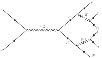
Figure 1: Pair-production of heavy charged fermions ($\psi^{+}\psi^{-}$) and their subsequent decay at an $e^{+}\,e^{-}$ collider.

We illustrate the method using a simple model where the NP consists of heavy charged and neutral fermions, $\psi^{\pm}$ and $\psi_{0}$, respectively, having $\psi_{0}\psi^{\pm}W^{\mp}$ coupling. These particles appear in extensions of the SM with a fermion isodoublet $\Psi=\left(\psi^{0},\psi^{-}\right)^{T}$ having hypercharge $Y_{\Psi}=-1$, specifically in a vector-like singlet-doublet model Bhattacharya:2015qpa , providing a viable dark matter (DM) in the form of $\psi^{0}$, when they are stabilized by a $Z_{2}$ symmetry. Here we take on a purely phenomenological approach, considering $\psi^{\pm}$ to have general chiral couplings to the $Z$ boson parameterized by two NP couplings, $a$ and $b$, but minimal coupling to photon Bhattacharya:2021ltd ,

$$\psi^{+}\psi^{-}Z:-~{}\frac{ie_{0}}{2s_{w}c_{w}}\gamma^{\mu}\left(a+b\gamma^{5}\right)\;,~{}\psi^{+}\psi^{-}\gamma:-~{}ie_{0}\gamma^{\mu}\,,$$ (10)

where $e_{0}$ is $U(1)_{\tt em}$ coupling constant, $s_{w}$ and $c_{w}$ are the cosine and sine of the weak mixing angle, respectively.

We now calculate the optimal (i.e. minimal) statistical uncertainty when measuring the NP couplings $a,\,b$ in the pair production of $\psi^{\pm}$ (with their subsequent decays) at an $e^{+}e^{-}$ collider (see Fig. 1):

$$e^{+}e^{-}\rightarrow\psi^{+}\psi^{-}\rightarrow W^{+}W^{-}\psi_{0}\bar{\psi}_{0}~{},~{}W\rightarrow\ell\nu\,,$$ (11)

with $\ell=e,\,\mu$. We assume the $\psi_{0}(\bar{\psi_{0}})$ to be stable DM candidates that escapes detection, so that the signal consists of missing energy ($\not{E}=\sqrt{s}-E_{\rm vis}$) plus opposite sign dileptons (OSL) . We include all possible 2-body and 3-body SM backgrounds: $e^{+}e^{-}\rightarrow WW,\,ZZ,\,\mu\mu,\,\tau\tau,\,WWZ,\,\ell\ell Z$, with the subsequent leptonic decays of the $W,\,Z$ and $\tau$. In order to suppress the SM backgrounds we impose thee following cuts :

• $\mathcal{C}_{1}$: $p_{T}^{\ell}>10$ GeV, $N_{\tt lep}=2$, $|m_{\ell\ell}-m_{Z}|>15$ GeV and $\Delta R_{\ell\ell}<3.0$,

• $\mathcal{C}_{2}$: $\not{E}>325$ GeV ,

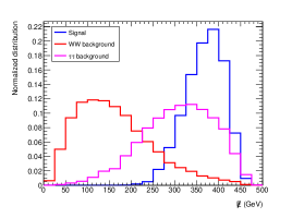
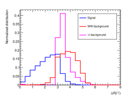
Figure 2: Normalized $\not{E}$ distribution (left) and $\Delta R(\ell^{+}\ell^{-})$ (right) for signal and dominating backgrounds of the reaction in Fig. 1; see text for details. We assumed $\sqrt{s}=500$ GeV, $m_{\psi^{\pm}}=210$ GeV (consistent with LEP bound L3:2001xsz ) and $m_{\psi_{1}}=60$ GeV.

where $N_{\tt lep}$ is the number of light charged leptons in the final state, $m_{\ell\ell}$ the invariant mass of the two final charged leptons, and $\Delta R=\sqrt{(\Delta\eta)^{2}+((\Delta\phi)^{2})}$ is the angular separation between two opposite sign leptons. $\mathcal{C}_{2}$ reduces the (dominant) $W$ background, while $\mathcal{C}_{1}$ suppresses the $Z,\,\mu$ and $\tau$ backgrounds; see Fig. 2.

We now determine the accuracy to which $a$ and $b$ can be measured, assuming these couplings have one of the following seed values: $\bullet$ $a^{0}=0$, $b^{0}=1$ (pure axial coupling), $\bullet$ $a^{0}=1$, $b^{0}=0$ (pure vector coupling), $\bullet$ $a^{0}=1$, $b^{0}=1$ (chiral coupling)  .

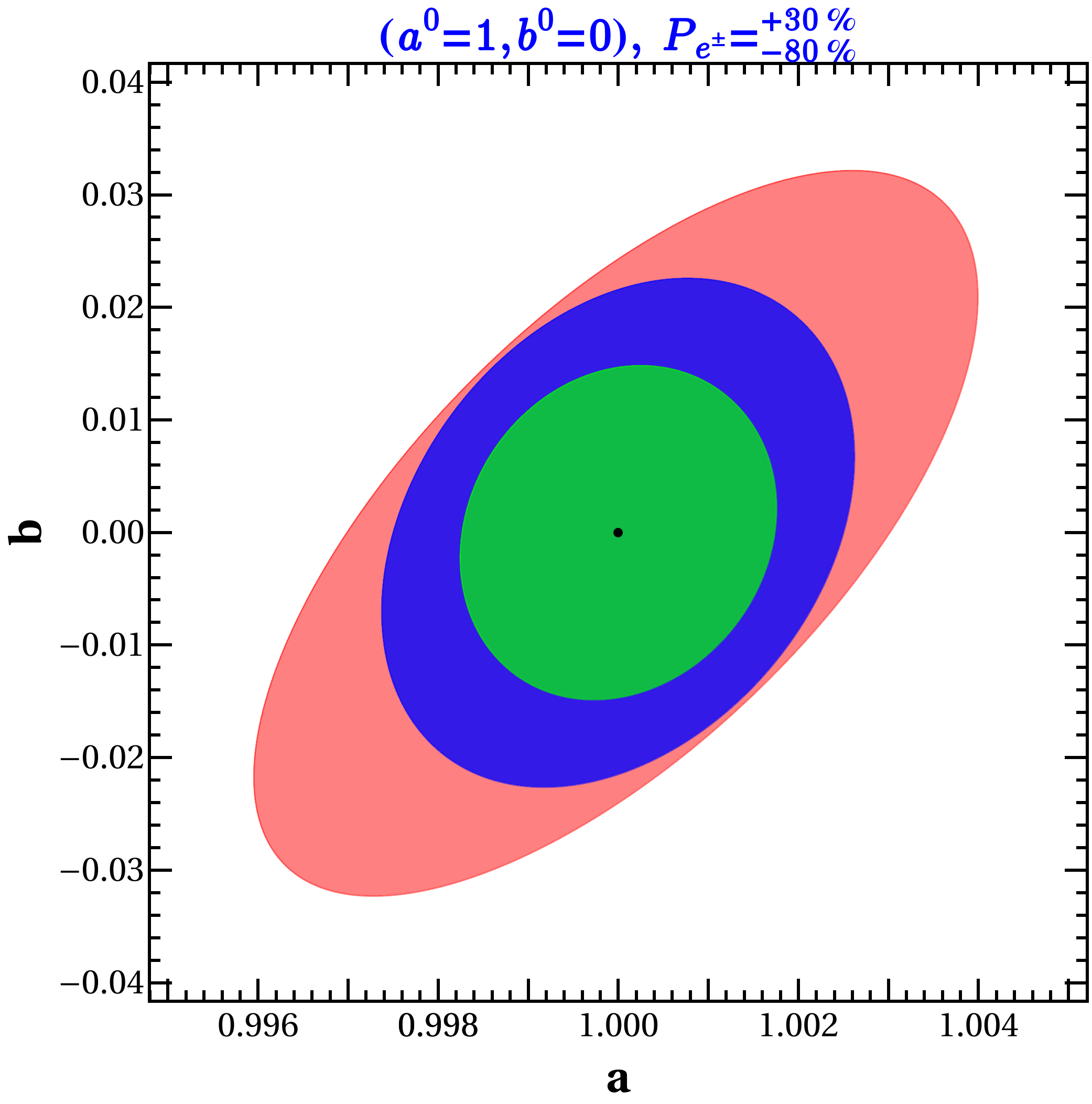
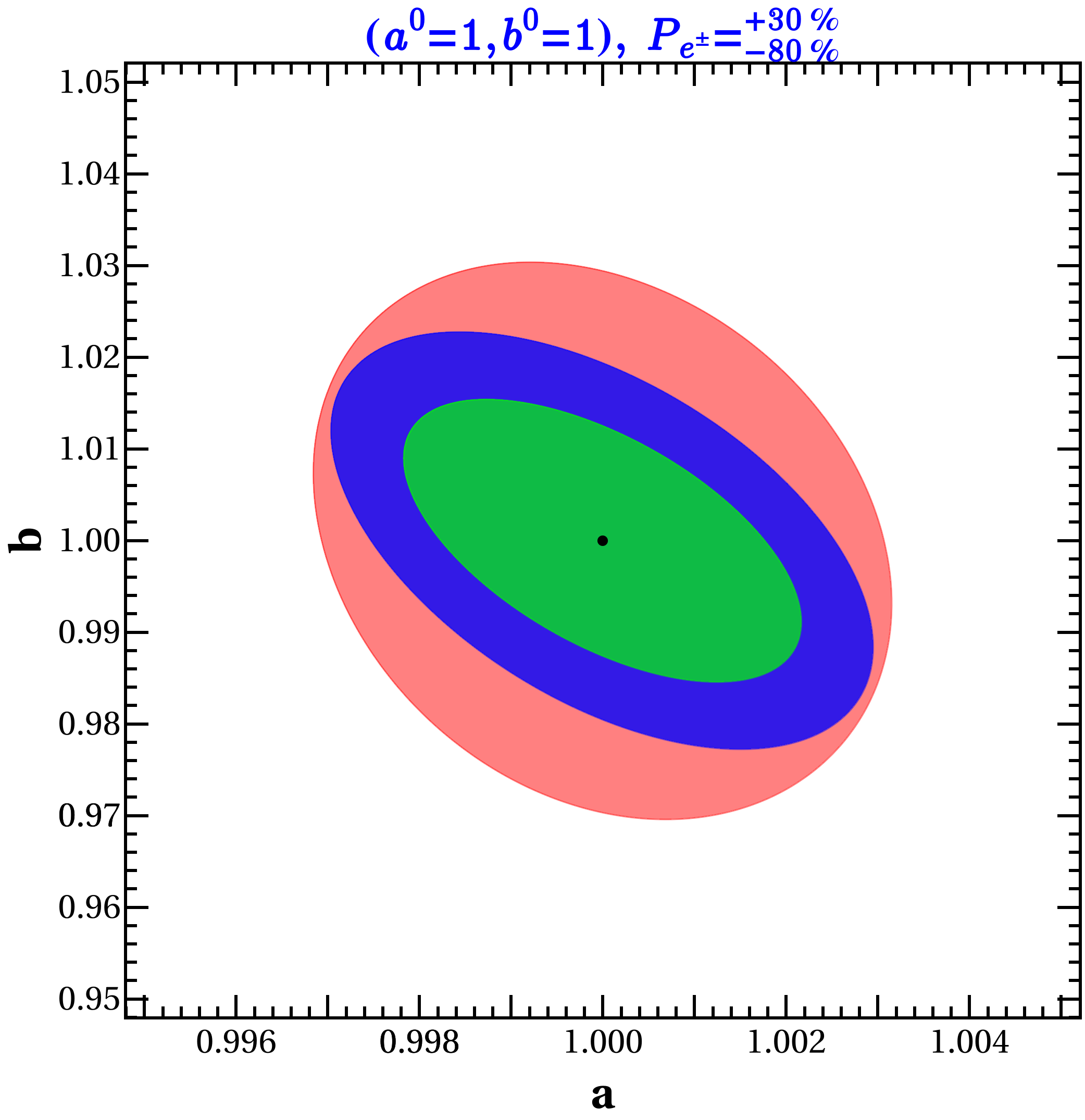
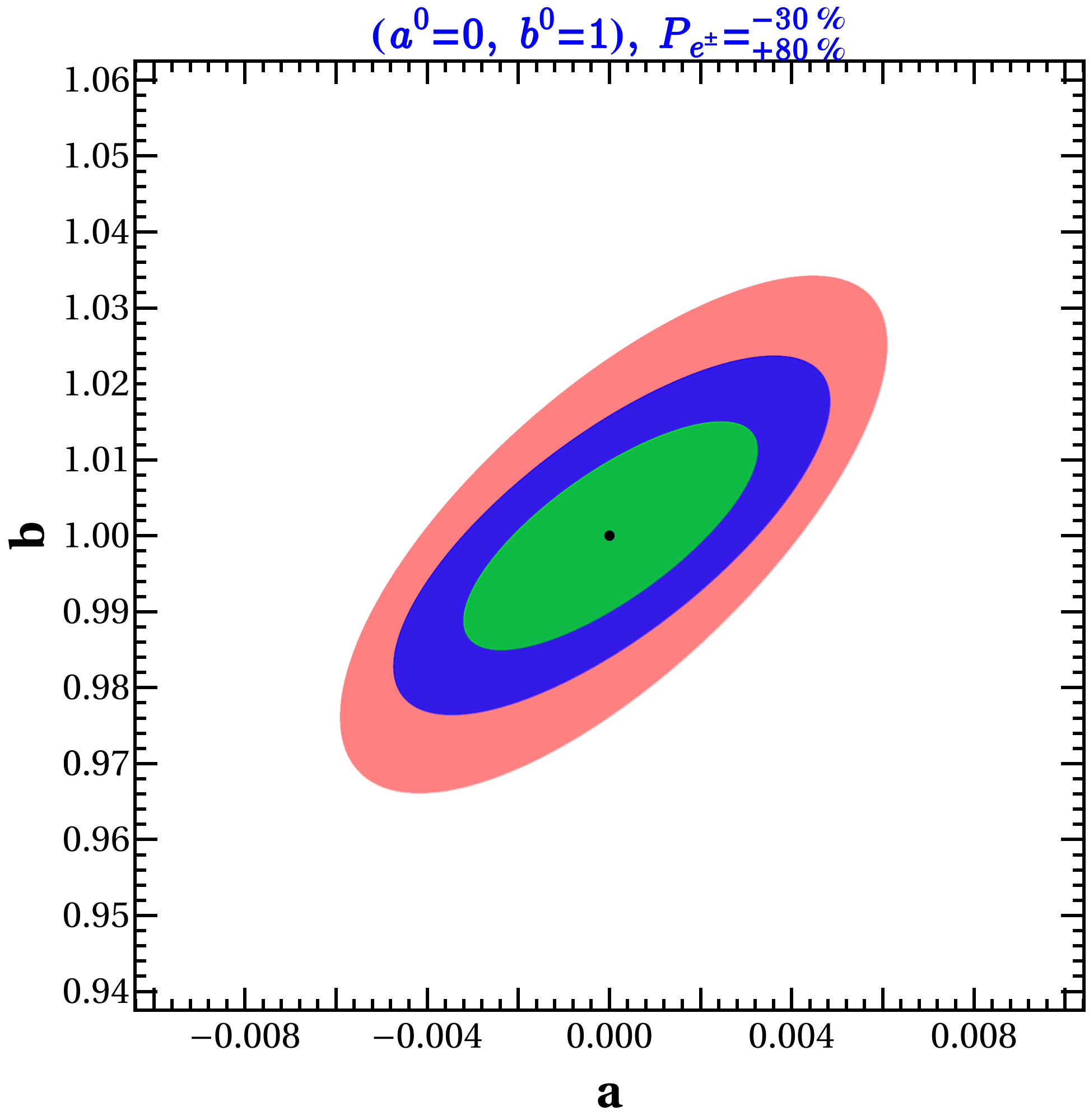
Figure 3: Effects of cuts on the 1$\sigma$ surfaces for 3 different hypotheses: signal only with $\mathcal{C}_{1}+\mathcal{C}_{2}$ applied (green); and signal+background after $\mathcal{C}_{1}$ (light read), and $\mathcal{C}_{1}+\mathcal{C}_{2}$ (blue) – see the text for details.

We list in table 1 the results for both signal and background event numbers, and the corresponding production cross sections (note that for this reaction there is no SM-DM interference); the results illustrate the effectiveness of the cuts imposed in reducing the background, and also the effects of the beam polarization. We assumed the the CM collider energy is $\sqrt{s}=500$ GeV and an integrated luminosity of ${\mathfrak{L}_{\tt int}}=2000~{}\rm{fb^{-1}}$, and took $m_{\psi^{\pm}}=210\,\text{GeV},\,m_{\psi_{0}}=60\,\text{GeV}$.

The choice of beam polarization plays a crucial role in optimizing signal to noise ratio, that in turn helps in reducing the uncertainty of the coupling estimates. For example, the choice $P_{e^{\pm}}=^{+30\%}_{-80\%}$ (consistent with the ILC design Behnke:2013xla ), increases the signal cross-section when $a^{0}=1,\,b^{0}=0$ (it also increases the $WW$ background, but this is suppressed by $\mathcal{C}_{2}$); this results in smaller uncertainties than those obtained using unpolarized beams. For $a^{0}=0,b^{0}=1$ the choice $P_{e^{\pm}}=^{-30\%}_{+80\%}$ enhances the signal cross-section, and also suppresses the $WW$ background.

Processes	Production cross-section		Number of events
	after $\mathcal{C}_{1}$ (fb)		after $\mathcal{C}_{1}$ and $\mathcal{C}_{2}$
	$P_{e^{\pm}}=^{-30\%}_{+80\%}$	$P_{e^{\pm}}=^{+30\%}_{-80\%}$	$P_{e^{\pm}}=^{-30\%}_{+80\%}$	$P_{e^{\pm}}=^{+30\%}_{-80\%}$
$a^{0}=1,b^{0}=0$	5.2	55.7	4791	50832
$a^{0}=0,b^{0}=1$	19.6	20.4	17685	18479
$a^{0}=1,b^{0}=1$	7.0	58.2	6457	53250
$WW$	51	798	1558	18030
$\tau\tau/\mu\mu$	57	68	286	360
$ZZ$	8.8	18.9	21	44
$\nu\nu Z$	3.4	50	72	1190
$\ell\ell Z$	16.5	22.4	18	4
$WWZ$	0.063	0.87	21	248

Table 1: Production cross sections with $\mathcal{C}_{1}$ imposed and final event numbers after cuts $\mathcal{C}_{1}+\mathcal{C}_{2}$, for signal and background contributions to the reaction in Fig. 1. We took CM energy $\sqrt{s}=500$ GeV, integrated luminosity ${\mathfrak{L}_{\tt int}}=2000~{}\rm{fb^{-1}}$ and two polarization choices; we assumed $m_{\psi^{\pm}}=210$ GeV and $m_{\psi_{0}}=60$ GeV.

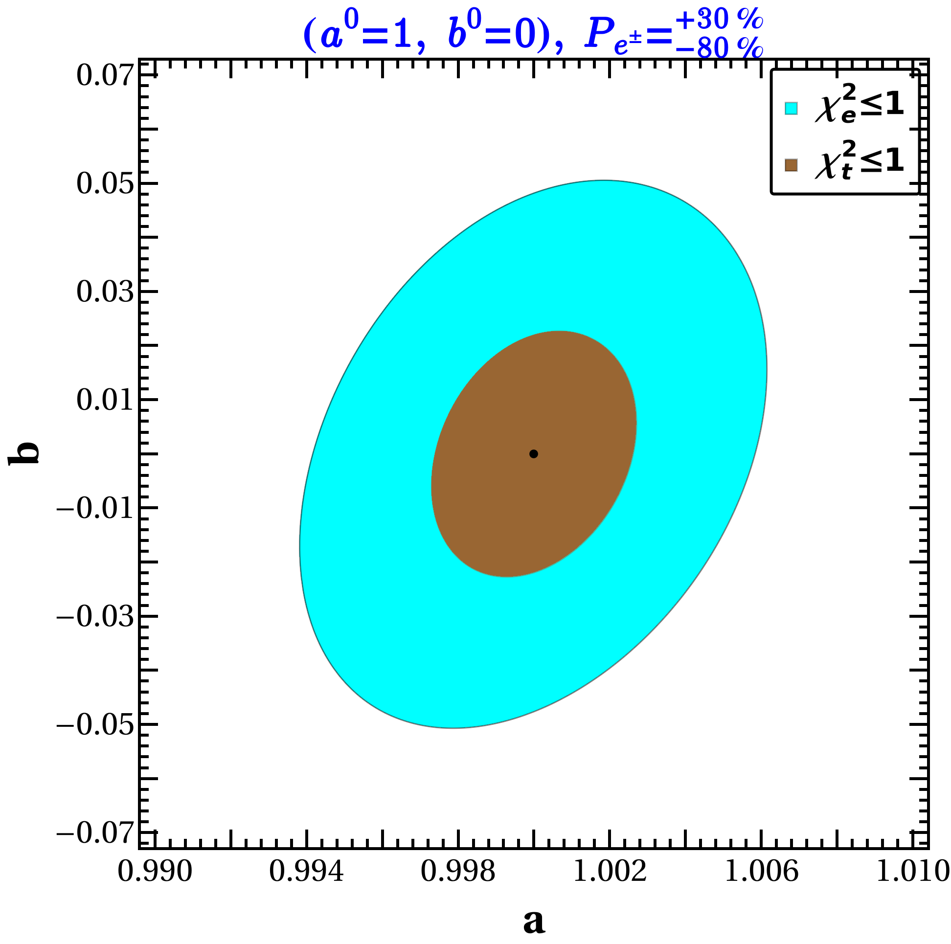
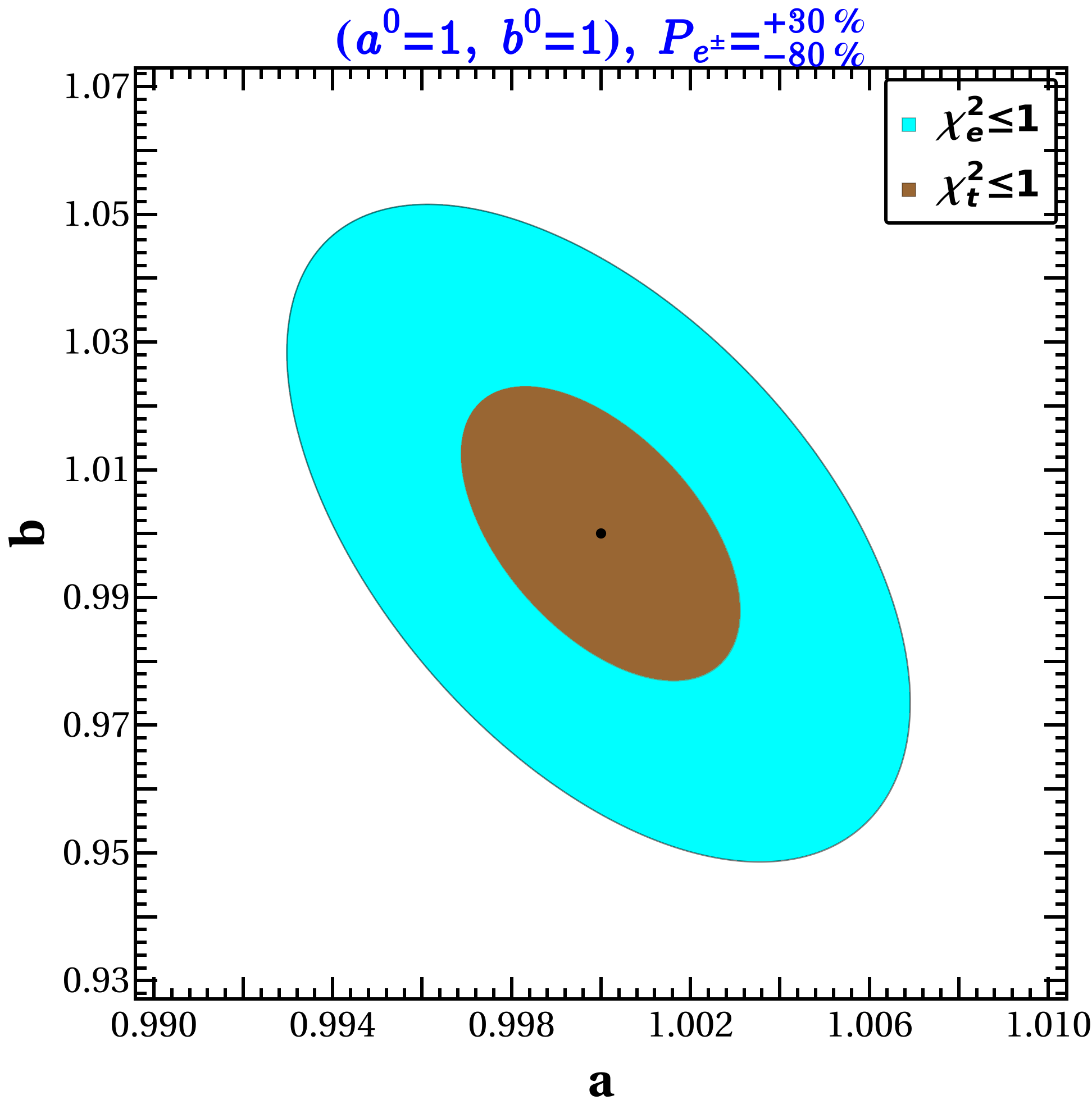
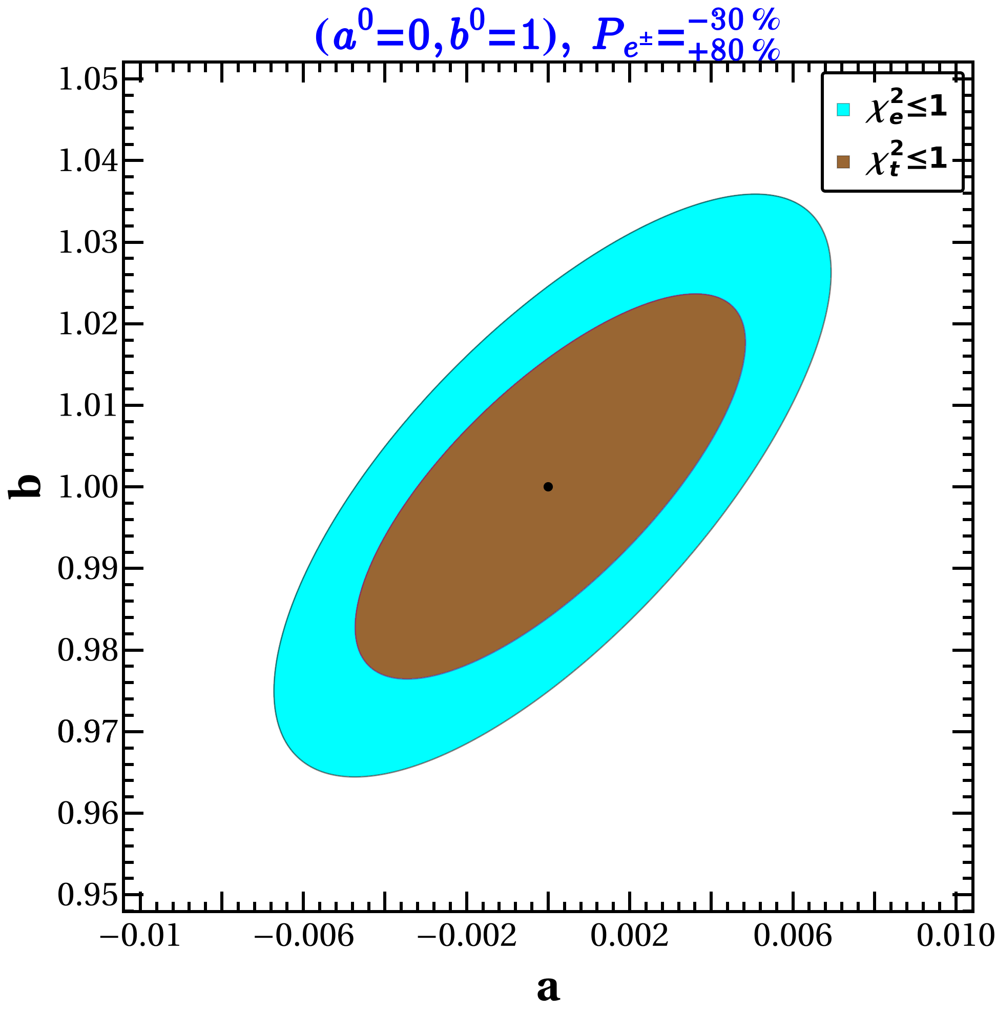
Figure 4: Comparison of 1$\sigma$ regions between standard approach (cyan) and OOT (brown) for three different hypotheses.

The 1$\sigma$ regions, defined by $\chi^{2}_{\tt t}\leq 1$ (cf. Eq. 3), for the three choices of $a^{0},\,b^{0}$ considered above, are shown in the Fig. 3, for the signal-only with $\mathcal{C}_{1}$ and $\mathcal{C}_{2}$ imposed (green), for the full signal and background after applying $\mathcal{C}_{1}$ only (light red), and for the full signal plus background after applying $\mathcal{C}_{1}$ and $\mathcal{C}_{2}$ (blue). This illustrates the degradation of the (optimal) precision to which the NP parameters can be estimated once the background is included (a feature absent in several previous analyses that used the OOT).

It should be noted that the shape and orientation of the 1$\sigma$ ellipses has a complicated dependence on the NP parameters $a^{0},\,b^{0}$, as well as on the polarization and the specific choices made for $\mathcal{C}_{1,2}$. These features cannot be mimicked using an efficiency factor multiplying the signal and background cross sections. Such a simplification is appropriate when the background is ignorable, or when the cuts reduce signal and background events without changing their phase-space correlation, which occurs in a limited number of situations. In general, it is more accurate and reliable to follow the above procedure than the efficiency approximation.

We now turn to the basic question we wish to address, namely, how close does a standard analysis of collider data come to the OOT results when extracting parameter uncertainties? This standard approach is, in general, based on the $\chi^{2}_{\tt e}$ function, defined as,

$$\chi^{2}_{\tt e}=\sum_{k}\left(\frac{N^{\text{exp}}_{k}-N^{\text{theo}}_{k}(a,b)}{\sqrt{N^{\text{exp}}_{k}}}\right)^{2}\,,$$ (12)

where $N_{k}^{\text{theo}}$ denotes the number of events in the $k^{\tt th}$ bin predicted by the model (after applying the cuts $\mathcal{C}_{1}$ and $\mathcal{C}_{2}$), and $N^{\text{exp}}$ the corresponding number of events generated by a simulation of the model with paramters $a^{0},\,b^{0}$.

In Fig. 4, we present a comparison of the the 1$\sigma$ regions from both OOT and regular $\chi^{2}_{\tt e}$ analyses for three different hypotheses listed above. The figures also provide a measure of the level of improvement needed in the regular $\chi_{\tt e}^{2}$ analysis to reach the minimal uncertainties derived using the OOT; the reason the $\chi^{2}_{\tt e}$ result is close to the optimal on for $a^{0}=0,\,b^{0}=1$ is that in this case the background is the smallest, whence the event distribution closely mimics the pure signal. This situation will repeat in all cases where the signal dominates over the background.

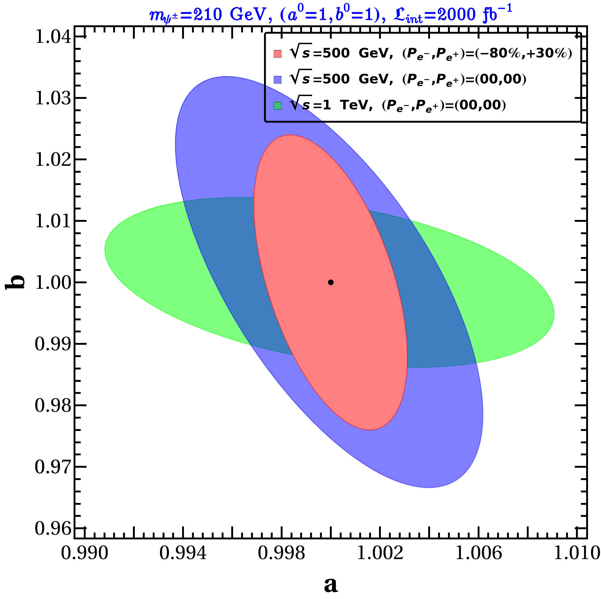
Figure 5: Comparison of 1$\sigma$ surfaces for different CM energy and beam polarization.

It is worthwhile studying how the uncertainty and correlation of NP couplings depend on the CM energy and beam polarization. An illustrative example is presented in Fig. 5, from which we can infer that the covariance matrix can be strongly dependent on $\sqrt{s}$ (for this particular case, the uncertainty in $b$ drops, while that in $a$ enhances with larger $\sqrt{s}$); while, as noted previously, the overall uncertainty can be significantly reduced by an appropriate choice of polarization. The ability of the OOT to determine the changes in precision to which NP parameters can be extracted with both polarization and CM energy provides a useful guide in selecting future collider designs.

In summary, we provide a simple and general numerical method for the application of the OOT to collider processes. This approach allows determination of the maximal statistical precision that can be reached when measuring NP parameters in any given collider process, incorporating all experimental cuts to reduce the background. The results obtained provide a useful gauge of the degree of optimization reached by standard data analysis techniques, and of the effects of collider parameters, such as CM energy and beam polarization (when available) in the precision that can be reached. This last can be used to compare different collider proposals, for example, a $\mu^{+}\mu^{-}$ collider with relatively high CM energy, but no polarized beam, against an $e^{+}e^{-}$ collider of lower energy but with polarized beams. Finally, we reiterate that the approach described here is much preferable to the “efficiency approximation” where experimental cuts and branching ratios are mimicked by multiplying the hard cross sections by a fixed factor.

Acknowledgement SB acknowledges the grant CRG/2019/004078 from DST-SERB, Govt. of India.

SUPPLEMENTAL MATERIAL

I Singlet doublet model and dark matter phenomenology

The singlet-doublet dark matter model is one of the simplest extensions of the SM consisting of two additional vector-like leptons: a $SU(2)$ doublet, $\Psi=(\psi_{1},\,\psi^{-}\,)$ of hypercharge $Y=-1$, and a singlet $\chi$ of zero hypercharge. Both $\psi$ and $\chi$ are assumed odd under a discrete $\mathbbm{Z}_{2}$ symmetry, while all the SM fields are even. Following electroweak symmetry breaking (EWSB), the $\psi\chi H$ Yukawa coupling (cf. Eq. (13) below) induces a mixing of the neutral component $\psi^{0}$ and $\chi$; the lighter mass eigenstate will serve as a viable DM candidate. The quantum numbers under SM$\times\mathbbm{Z}_{2}$ symmetry are summarized in Table 2.

field	$SU(3)_{\tt C}$	$SU(2)_{\tt L}$	$U(1)_{\tt Y}$	$\mathbbm{Z}_{2}$
$\Psi$	$1$	$2$	$-1$	$-$
$\chi$	$1$	$1$	$0$	$-$

Table 2: Quantum numbers of dark-sector fermions under ${\rm SU(3)}_{\tt C}\times{\rm SU(2)}_{\tt L}\times{\rm U(1)}_{\tt Y}\times\mathbbm{Z}_{2}$. SM fields are even under $\mathbbm{Z}_{2}$.

The Lagrangian of the model is given by

$$\mathcal{L}^{\tt VF}=\bar{\Psi}\left[i\left(\not{\partial}-i\frac{g}{2}\sigma^{a}W_{\mu}^{a}-ig^{\prime}\frac{Y}{2}B_{\mu}\right)-m_{\psi^{\pm}}\right]\Psi+\bar{\chi}\left(i\not{\partial}-m_{\chi}\right)\chi-\left(y\bar{\Psi}\widetilde{H}\chi+\text{H.c}\right)\,,$$ (13)

where $H$ is SM Higgs doublet, $B_{\mu}$ and $W_{\mu}$ are the ${\rm U(1)}_{Y}$ and ${\rm SU(2)}_{L}$ gauge fields, and $g,\,g^{\prime}$ are the corresponding gauge couplings. After EWSB, $H$ acquires a vev  $v/\sqrt{2}$, and the mass term for dark fermions can be written as,

$$-\mathcal{L}_{\tt mass}=\left(\bar{\chi},\bar{\psi}_{1}\right)\begin{pmatrix}m_{\chi}&\mu\cr\mu&m_{\psi^{\pm}}\end{pmatrix}\begin{pmatrix}\chi\cr\psi_{1}\end{pmatrix}+m_{\psi^{\pm}}{\psi^{+}}\psi^{-};\qquad\mu=\frac{yv}{\sqrt{2}}\,.$$ (14)

The mass eigenstates $\psi_{0}$ and $\psi_{0}^{{}^{\prime}}$ are then

$$\begin{pmatrix}\chi\\ \psi_{1}\end{pmatrix}=\begin{pmatrix}\cos\gamma&\sin\gamma\\ -\sin\gamma&\cos\gamma\end{pmatrix}\begin{pmatrix}\psi_{0}\\ \psi_{0}^{{}^{\prime}}\end{pmatrix};\qquad\tan 2\gamma=\frac{2\mu}{m_{\chi}-m_{\psi^{\pm}}}.$$ (15)

We will assume  $|\mu|\ll m_{\chi}<m_{\psi^{\pm}}$ such that $2\mu\ll|m_{\chi}-m_{\psi^{\pm}}|$; in this case $\gamma$ is small and

$$m_{\psi_{0}}\simeq m_{\chi}-\frac{\mu^{2}}{m_{\psi^{\pm}}-m_{\chi}}\,,\qquad m_{\psi_{0}^{{}^{\prime}}}\simeq m_{\psi^{\pm}}+\frac{\mu^{2}}{m_{\psi^{\pm}}-m_{\chi}};$$ (16)

therefore $m_{\psi_{0}^{{}^{\prime}}}>m_{\psi^{\pm}}>m_{\psi_{0}}$ and $\psi_{0}$ is the DM candidate.

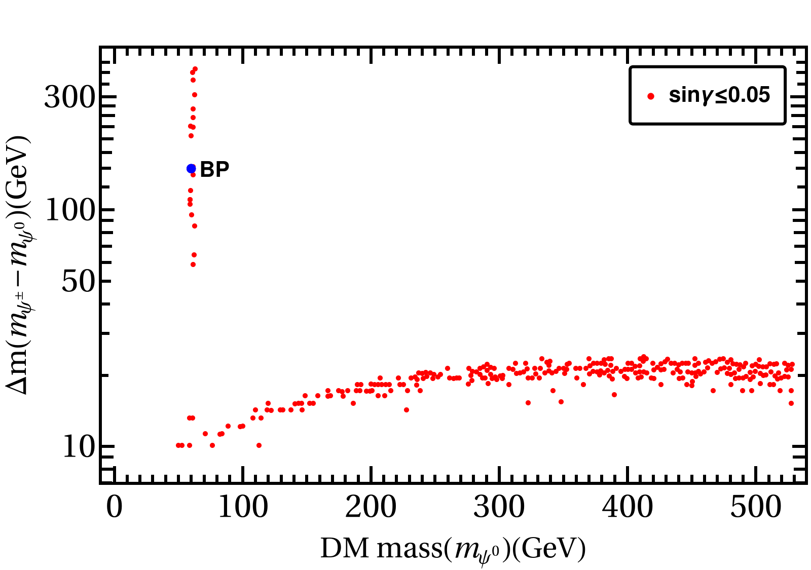
Figure 6: Relic density and direct search allowed parameter space in $\Delta m$ vs $m_{\psi_{0}}$ plane for singlet-doublet dark matter model. The choice of the benchmark point used in the main analysis is indicated.

We see that the charged heavy fermions (${\psi^{\pm}}$) have vector-like interactions with $Z$ boson (corresponding $a^{0}=c_{2\tt w}\sim 1/2,\,b^{0}=0$) which is similar to one of our hypotheses ($a^{0}\neq 0$, $b^{0}=0$) as described in the main text. $\Delta m$, $m_{\psi_{0}}$ and $\sin\gamma$ are the free parameters of the model and govern its DM phenomenology. The parameter space in the $\Delta m$ vs $m_{\psi_{0}}$ plane allowed by relic density and direct search constraints is shown in Fig. (6), along with the choice of a benchmark point that corresponds to the values of $m_{\psi^{0},\,\psi^{\pm}}$ used in the main text. The freedom in choosing $\Delta m$ around $m_{\psi_{0}}\sim m_{h}/2\sim 62.5$ GeV, is due to the effects of the Higgs resonance, while in other regions, co-annihilation dependence keeps a tight correlation between $\Delta m$ and $m_{\psi_{0}}$.

II Signal and background cross-sections for different choices of beam polarization

We now consider the reaction used in the main text: $e^{+}e^{-}\rightarrow\psi^{+}\psi^{-}$. The dependence the cross section on $\sqrt{s}$ for three different hypotheses and for different choices of beam polarization is shown in the top panel of Fig. (7). For $a=1,b=0$, $P_{e^{\pm}}=^{+30\%}_{-80\%}$ beam polarization combination, enhances the total production cross-section compared to unpolarized beams due to the effects of the vector coupling of $\psi^{\pm}$ with $Z$. For $a=1,b=1$, the enhancement in the total cross-section is comparatively modest due to the decrease in the total cross-section resulting from the axial vector current. For the purely axial-vector like case $a=0,b=1$, due to the photon mediation, total cross-section increases while axial-vector current leads to a decrease in cross-section for $P_{e^{\pm}}=^{+30\%}_{-80\%}$ polarization combination. If we flip the sign of the beam polarization, the case is reversed. This exemplifies the significance of beam polarization when studying these different models.

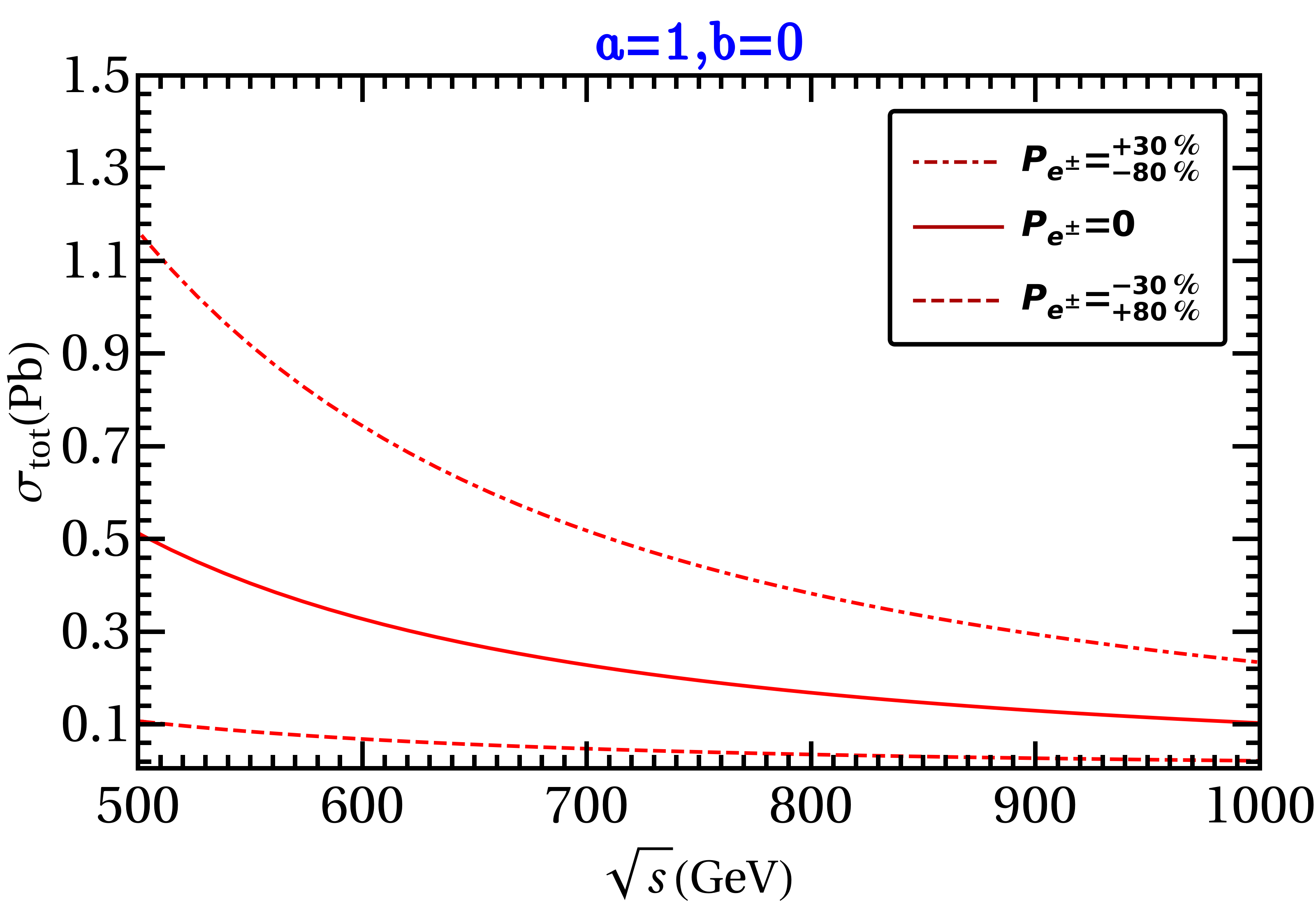
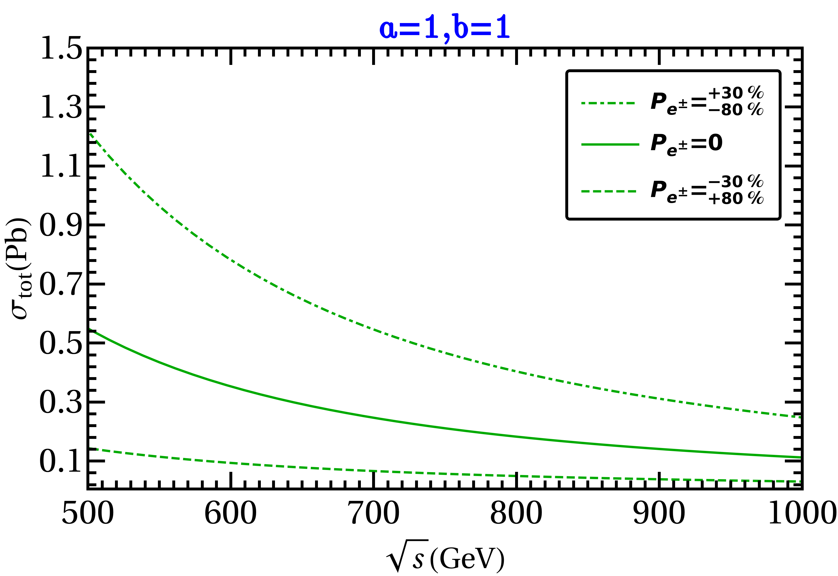
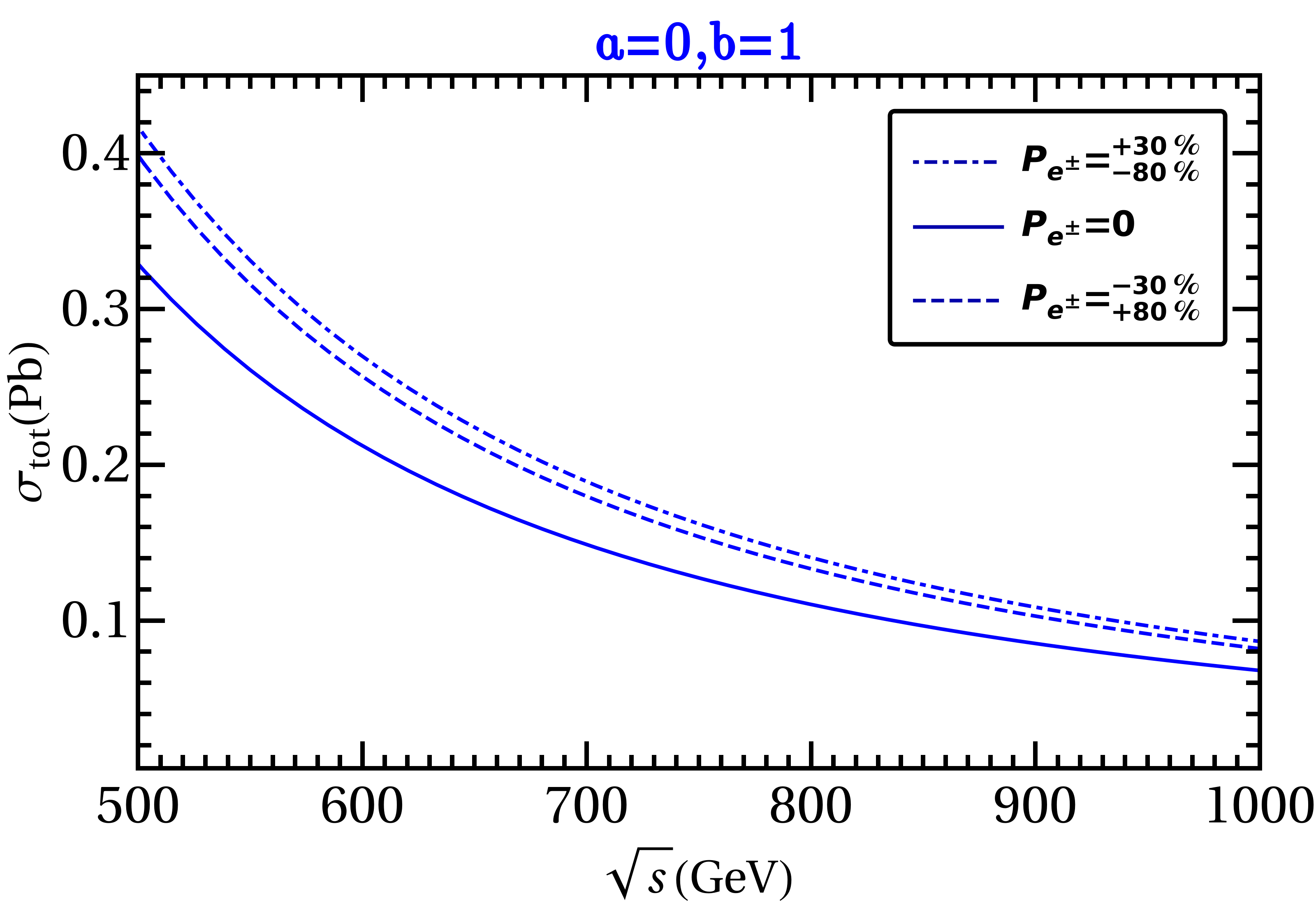
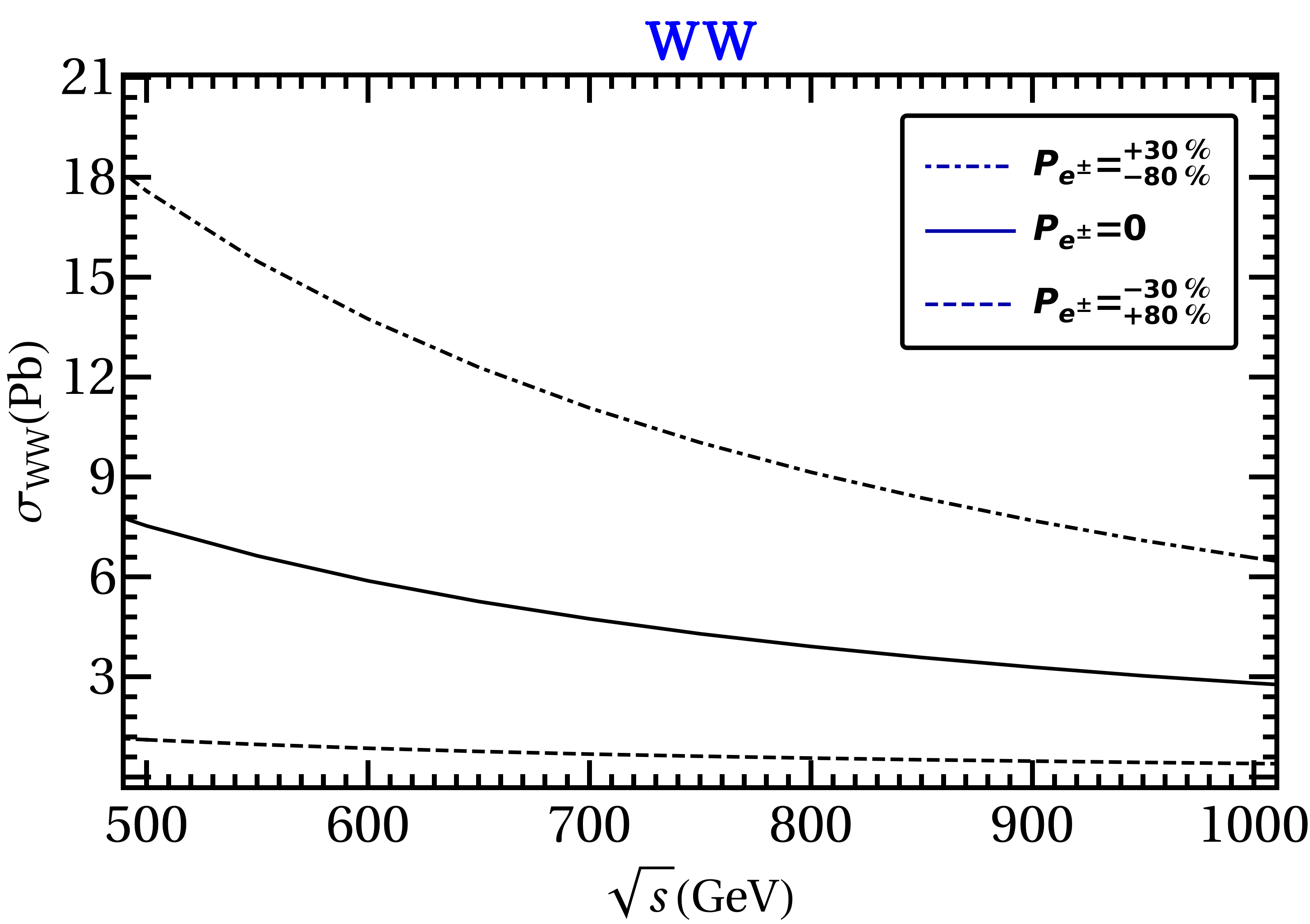
Figure 7: Top: The variation of the total cross-section for the signal with CM energy for different choices of beam polarization. Bottom: Same for the $WW$ background. Beam polarization choices are as indicated in the inset of each figure.

The major SM background contribution to the final state signal of two opposite-sign leptons+ missing energy arises from $WW$ production; in $e^{+}e^{-}$ colliders this occurs through $s$-channel photon and $Z$, and $t$-channel neutrino exchange. For $P_{e^{\pm}}=^{+30\%}_{-80\%}$ combination, the $WW$ cross-section increases compared to unpolarized beam. If we flip the polarization sign, $WW$ cross-section drops, as depicted in the bottom panel of Fig. (7).

References

- (1) M. Diehl and O. Nachtmann, Z. Phys. C 62, 397-412 (1994) doi:10.1007/BF01555899
- (2) J. F. Gunion, B. Grzadkowski and X. G. He, Phys. Rev. Lett. 77, 5172-5175 (1996) doi:10.1103/PhysRevLett.77.5172 [arXiv:hep-ph/9605326 [hep-ph]].
- (3) S. Bhattacharya, S. Jahedi and J. Wudka, JHEP 05, 009 (2022) doi:10.1007/JHEP05(2022)009 [arXiv:2106.02846 [hep-ph]].
- (4) B. Grzadkowski and Z. Hioki, Phys. Lett. B 391, 172-176 (1997) doi:10.1016/S0370-2693(96)01439-6 [arXiv:hep-ph/9608306 [hep-ph]].
- (5) B. Grzadkowski, Z. Hioki and M. Szafranski, Phys. Rev. D 58, 035002 (1998) doi:10.1103/PhysRevD.58.035002 [arXiv:hep-ph/9712357 [hep-ph]].
- (6) J. F. Gunion and J. Pliszka, Phys. Lett. B 444, 136-141 (1998) doi:10.1016/S0370-2693(98)01364-1 [arXiv:hep-ph/9809306 [hep-ph]].
- (7) B. Grzadkowski and Z. Hioki, Phys. Rev. D 61, 014013 (2000) doi:10.1103/PhysRevD.61.014013 [arXiv:hep-ph/9805318 [hep-ph]].
- (8) B. Grzadkowski and J. Pliszka, Phys. Rev. D 60, 115018 (1999) doi:10.1103/PhysRevD.60.115018 [arXiv:hep-ph/9907206 [hep-ph]].
- (9) B. Grzadkowski and Z. Hioki, Nucl. Phys. B 585, 3-27 (2000) [erratum: Nucl. Phys. B 894, 585-587 (2015)] doi:10.1016/j.nuclphysb.2015.03.020 [arXiv:hep-ph/0004223 [hep-ph]].
- (10) K. Hagiwara, S. Ishihara, J. Kamoshita and B. A. Kniehl, Eur. Phys. J. C 14, 457-468 (2000) doi:10.1007/s100520000366 [arXiv:hep-ph/0002043 [hep-ph]].
- (11) B. Grzadkowski, Z. Hioki, K. Ohkuma and J. Wudka, Phys. Lett. B 593, 189-197 (2004) doi:10.1016/j.physletb.2004.04.075 [arXiv:hep-ph/0403174 [hep-ph]].
- (12) B. Grzadkowski, Z. Hioki, K. Ohkuma and J. Wudka, JHEP 11, 029 (2005) doi:10.1088/1126-6708/2005/11/029 [arXiv:hep-ph/0508183 [hep-ph]].
- (13) Z. Hioki, T. Konishi and K. Ohkuma, JHEP 07, 082 (2007) doi:10.1088/1126-6708/2007/07/082 [arXiv:0706.4346 [hep-ph]].
- (14) S. Dutta, K. Hagiwara and Y. Matsumoto, Phys. Rev. D 78, 115016 (2008) doi:10.1103/PhysRevD.78.115016 [arXiv:0808.0477 [hep-ph]].
- (15) S. Jahedi and J. Lahiri, JHEP 04, 085 (2023) doi:10.1007/JHEP04(2023)085 [arXiv:2212.05121 [hep-ph]].
- (16) S. Bhattacharya, S. Jahedi and J. Wudka, JHEP 12 (2023), 026 doi:10.1007/JHEP12(2023)026 [arXiv:2301.07721 [hep-ph]].
- (17) S. Jahedi, JHEP 12 (2023), 031 doi:10.1007/JHEP12(2023)031 [arXiv:2305.11266 [hep-ph]].
- (18) T. Behnke, J. E. Brau, B. Foster, J. Fuster, M. Harrison, J. M. Paterson, M. Peskin, M. Stanitzki, N. Walker and H. Yamamoto, [arXiv:1306.6327 [physics.acc-ph]].
- (19) P. Achard et al. [L3], Phys. Lett. B 517, 75-85 (2001) doi:10.1016/S0370-2693(01)01005-X [arXiv:hep-ex/0107015 [hep-ex]].
- (20) S. Bhattacharya, N. Sahoo and N. Sahu, Phys. Rev. D 93, no.11, 115040 (2016) doi:10.1103/PhysRevD.93.115040 [arXiv:1510.02760 [hep-ph]].