The entanglement membrane in exactly solvable lattice models

Abstract

Entanglement membrane theory is an effective coarse-grained description of entanglement dynamics and operator growth in chaotic quantum many-body systems. The fundamental quantity characterizing the membrane is the entanglement line tension. However, determining the entanglement line tension for microscopic models is in general exponentially difficult. We compute the entanglement line tension in a recently introduced class of exactly solvable yet chaotic unitary circuits, so-called generalized dual-unitary circuits, obtaining a non-trivial form that gives rise to a hierarchy of velocity scales with $v_{E}<v_{B}$. We find that these circuits saturate certain bounds on entanglement growth that are also saturated in holographic models. Furthermore, we relate the entanglement line tension to temporal entanglement and correlation functions. We also find new methods of constructing generalized dual-unitary gates beyond qubits that display behavior unique to local dimension $\geq 3$. Our results shed light on entanglement membrane theory in microscopic Floquet lattice models and enable us to perform non-trivial checks on the validity of its predictions by comparison to exact and numerical calculations.

I Introduction

Effective descriptions form the backbone of our understanding of modern condensed matter physics [1]. Rather than considering a full microscopic description of a many-body system, which is both intractable and uninstructive, it is generally possible to identify the most relevant degrees of freedom through an effective ‘coarse-graining’. In this way the important features of the model, determining its macroscopic behavior, can be determined from a tractable theory for the emergent effective degrees of freedom. In equilibrium statistical physics these features are typically the symmetry and topology of the Hamiltonian.

Recent years have seen a substantial increase in our understanding of the universal aspects of non-equilibrium quantum dynamics [2, 3]. Somewhat surprisingly, it has turned out that even chaotic dynamics, i.e., non-integrable dynamics lacking any global symmetries, displays universal macroscopic behaviors that can be captured in a hydrodynamic description. Prime examples are the emergence of a hydrodynamics of information transport with information acting as the conserved quantity [4, 5], or the appearance of Kardar-Parisi-Zhang scaling in the fluctuations of entanglement growth in noisy systems [6].

Entanglement membrane theory (EMT) unifies the examples mentioned above and provides an effective coarse-grained description of the macroscopic aspects of chaotic quantum many-body dynamics [6, 7]. It is based on the observation that in such non-integrable dynamics entanglement is produced locally, as opposed to being transported by stable quasiparticles – as is the case in integrable dynamics. The effective theory for the “entanglement membrane” describing the dynamics is determined by the entanglement line tension (ELT). This line tension $\mathcal{E}(v)$ constitutes a local cost function for an entanglement membrane in spacetime and depends on a local velocity $v$. The leading-order behavior of entanglement dynamics and operator growth on sufficiently large length scales is then captured by the membrane configuration minimizing the total cost. In this way the quantum many-body problem can be reduced to standard statistical mechanics. This approach has been generalized to settings involving measurements, couplings to the environment, and Clifford circuits [8, 9, 10, 11]. However, determining the ELT from a microscopic model is generally hard. It has so far only been accomplished for random circuits in the large-local-Hilbert-space limit [6, 12], for certain holographic models [13, 14], and for dual-unitary circuits [12] (the only case of non-random Floquet spin models). While in the latter case the entanglement dynamics remain tractable, the ELT becomes trivial. Here we provide exact results for the ELT in a class of hierarchical dual-unitary circuits with nontrivial results, again avoiding the need for randomness or averaging.

I.1 Unitary circuits

Unitary circuits are discrete-space, discrete-time models for local unitary dynamics motivated by classical cellular automata [3]. Such circuits have gained much attention in recent years both theoretically and experimentally, since they present minimal models for many-body dynamics that can be naturally realized in current quantum computing setups [15, 16].

The basic building blocks of unitary circuits are two-site unitary gates $U$, whose matrix elements $U_{ab,cd}$ are graphically expressed as

(1)

If indices are suppressed, closed lines correspond to tensor contractions and open legs correspond to uncontracted indices (see also Ref. [3]). Moving from a two-site setting to a full one-dimensional lattice, a many-body evolution operator can be constructed by arranging the two-site unitary gates in a brickwork geometry as

$$\vbox{\hbox{\includegraphics[width=303.53267pt]{figs/diag_brickcircuit.pdf}}}\,.$$ (2)

Here discrete time runs vertically and the local degrees of freedom, e.g. qubits, are arranged horizontally, with unitary gates acting alternately on the even and odd bonds between them.

When considering entanglement properties it is often convenient to work in a “folded” space of replicated gates. For any number of replicas $\alpha$ the folded gate is graphically expressed as

$$\vbox{\hbox{\includegraphics[width=43.36464pt]{figs/folded_gate.png}}}\,=(U\otimes U^{*})^{\otimes\alpha},\quad\alpha=1,2,3,\ldots$$ (3)

We will make frequent use of the following vectors in the folded space

$$\vbox{\hbox{\includegraphics[height=12.64415pt]{figs/circle.png}}}\,=\frac{1}{q^{\frac{\alpha}{2}}}\,\overbrace{\vbox{\hbox{\includegraphics[height=12.64415pt]{figs/circle_renyi.png}}}}^{2\alpha}\,,\qquad\vbox{\hbox{\includegraphics[height=12.64415pt]{figs/square.png}}}\,=\frac{1}{q^{\frac{\alpha}{2}}}\,\overbrace{\vbox{\hbox{\includegraphics[height=12.64415pt]{figs/square_renyi.png}}}}^{2\alpha}\,.\,\,$$ (4)

Here we denote the local Hilbert space dimension by $q$, appearing as a normalization factor, and these two vectors correspond to permutations in replica space. The “circle”, , corresponds to the identity permutation and the “square”, , corresponds to the cyclic permutation.

Unitarity results in a set of graphical identities

$$\vbox{\hbox{\includegraphics[width=52.03227pt]{figs/unitarity_top.png}}}\,=\vbox{\hbox{\includegraphics[width=4.04489pt,angle={135}]{figs/circle.png}}}\,\vbox{\hbox{\includegraphics[width=4.04489pt,angle={225}]{figs/circle.png}}},\quad\vbox{\hbox{\includegraphics[width=52.03227pt]{figs/unitarity_bottom.png}}}\,=\vbox{\hbox{\includegraphics[width=4.04489pt,angle={45}]{figs/circle.png}}}\,\vbox{\hbox{\includegraphics[width=4.04489pt,angle={-45}]{figs/circle.png}}}.$$ (5)

The same equations hold when the cyclic permutation operator is used instead of the identity permutation operator . The same applies to the equations discussed in the following section.

I.2 Hierarchical generalization of dual unitarity

Dual-unitary gates [17, 18, 19, 20] satisfy an additional set of algebraic conditions that can be graphically represented as

$$\vbox{\hbox{\includegraphics[width=52.03227pt]{figs/dual_unitarity_l.png}}}\,=\begin{array}[]{c}\vbox{\hbox{\includegraphics[width=4.04489pt,angle={-45}]{figs/circle.png}}}\\ \vbox{\hbox{\includegraphics[width=4.04489pt,angle={-135}]{figs/circle.png}}}\end{array},\quad\vbox{\hbox{\includegraphics[width=52.03227pt]{figs/dual_unitarity_r.png}}}\,=\begin{array}[]{c}\vbox{\hbox{\includegraphics[width=4.04489pt,angle={45}]{figs/circle.png}}}\\ \vbox{\hbox{\includegraphics[width=4.04489pt,angle={135}]{figs/circle.png}}}\end{array}.$$ (10)

These identities result in a dynamics that is unitary not just along the discrete time direction but also along the spatial direction. Remarkably, dual-unitarity allow for the exact calculation a wide range of dynamical properties including correlation functions, operator dynamics, and entanglement growth, even though the resulting circuits are generically chaotic [19, 21, 22, 23, 24]. While most features of dual-unitary dynamics are in a sense “generic”, the operator dynamics is known to be pathological [25, 26].

The hierarchical generalization of dual unitarity is a recent attempt to find models which retain some of the solvability of dual-unitary circuits while avoiding the pathological features thereof [27]. It is also an attempt to unify models which are solvable by different means. The first level of the hierarchy, $\mathcal{L}_{1}$, is the set of dual-unitary gates. The second level of the hierarchy, $\mathcal{L}_{2}$, is defined by the algebraic conditions

$$\vbox{\hbox{\includegraphics[height=69.38078pt]{figs/L2_left_lhs.png}}}=\vbox{\hbox{\includegraphics[height=69.38078pt]{figs/L2_left_rhs.png}}},\quad\vbox{\hbox{\includegraphics[height=69.38078pt]{figs/L2_right_lhs.png}}}=\vbox{\hbox{\includegraphics[height=69.38078pt]{figs/L2_right_rhs.png}}}.$$ (11)

It encompasses the set $\mathcal{L}_{1}$, the set of product gates, and a class of gates locally equivalent to the CNOT gate (in particular also the CNOT gate itself). For qubits the above list is exhaustive, while there are also other examples for larger local Hilbert space dimension. Circuits composed out of CNOT gates have also been studied in the context of the Floquet quantum East model [28], where the above properties were used to obtain exact predictions for the thermalization and entanglement dynamics [29], and take a special place within this hierarchy since these gates are not just unitary but also T-dual: they satisfy

$$\vbox{\hbox{\includegraphics[width=52.03227pt]{figs/t_duality_l.png}}}\,=\begin{array}[]{c}\vbox{\hbox{\includegraphics[width=4.04489pt,angle={135}]{figs/circle.png}}}\\ \vbox{\hbox{\includegraphics[width=4.04489pt,angle={-45}]{figs/circle.png}}}\end{array},\quad\vbox{\hbox{\includegraphics[width=52.03227pt]{figs/t_duality_r.png}}}\,=\begin{array}[]{c}\vbox{\hbox{\includegraphics[width=4.04489pt,angle={-135}]{figs/circle.png}}}\\ \vbox{\hbox{\includegraphics[width=4.04489pt,angle={45}]{figs/circle.png}}}\end{array}.$$ (16)

This property is also satisfied by the set of product gates, i.e. two-site gates that are the direct product of two one-site unitary gates. It is an open question – which we answer in the positive – if gates that are neither dual-unitary nor T-dual exist in $\mathcal{L}_{2}$. We denote by $\bar{\mathcal{L}}_{2}$ the set of second level gates excluding dual-unitary gates. In contrast to dual-unitary circuits, whose correlations are supported exclusively on the light-cone edge, i.e. $x=vt$ with $v=1$, the correlations in $\bar{\mathcal{L}}_{2}$ circuits are also supported along the $v=0$ ray, i.e. at $x=0$. Everywhere else they vanish identically. However, for gates that are also T-dual all correlations of one-site operators along the $v=1$ ray aditionally vanish [23].

The $k$-th level of the hierarchy is defined by including $k$ gates in the algebraic condition. E.g., for $k=3$ the condition reads

$$\vbox{\hbox{\includegraphics[height=86.72267pt]{figs/L3_left_lhs.png}}}=\vbox{\hbox{\includegraphics[height=86.72267pt]{figs/L3_left_rhs.png}}}\,,\,\,\,\vbox{\hbox{\includegraphics[height=86.72267pt]{figs/L3_right_lhs.png}}}=\vbox{\hbox{\includegraphics[height=86.72267pt]{figs/L3_right_rhs.png}}}.$$ (17)

So far, due to the analytical and numerical challenges this equation poses, only few examples of $\bar{\mathcal{L}}_{3}$ gates exist, while nothing is known about $k\geq 4$. Little is known about the dynamics for $k\geq 3$.

I.3 Outline

This article is organized as follows. In Sec. II we compute the ELT in generalized dual-unitary circuits and discuss the physical implications of the result. Focusing first on $\bar{\mathcal{L}}_{2}$ circuits we extract the entanglement and butterfly velocity and discuss the relation of the particular simple form of the ELT to general bounds on entanglement growth. We show that the entanglement velocity is related to information spreading. Moreover, we discuss the relation of the ELT to influence matrices, thus providing a link to correlation functions. In this way the solvability of the $\bar{\mathcal{L}}_{2}$ circuits is related to the area-law (temporal) entanglement of the influence matrix. Finally, we generalize our results to $\bar{\mathcal{L}}_{k}$ circuits with $k\geq 3$ and show that solvability of both correlation functions and ELT is restricted to rays in spacetime with velocities $v_{*}\leq\lvert v\rvert\leq 1$. In Sec. III we verify the predictions of EMT with results extracted from probes of operator dynamics, focusing on the out-of-time-order correlator and the tripartite information. Furthermore, in Sec. IV we present numerical results on entanglement growth consistent with the predictions of EMT. Finally, in Sec. V we develop various methods to construct new $\bar{\mathcal{L}}_{2}$ gates based on constructions of gates with flat Schmidt spectrum. We explicitly construct $\bar{\mathcal{L}}_{2}$ gates which are not T-dual in local dimension $q=4$.

II Entanglement line tension

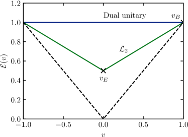
Figure 1: In $\bar{\mathcal{L}}_{2}$ circuits the ELT assumes a linear form. In constrast to dual-unitary circuits the slope is nonzero and $\bar{\mathcal{L}}_{2}$ circuits are thus characterized by an entanglement velocity $v_{E}<1$. Both $\bar{\mathcal{L}}_{2}$ and dual-unitary circuits have a maximal butterfly velocity $v_{B}=1$.

In this section we show that the ELT can be computed exactly for all velocities in $\bar{\mathcal{L}}_{2}$ circuits and for a range of velocities in higher levels of the hierarchy. Two velocities that can be directly extracted from the ELT are the entanglement velocity $v_{E}$, setting the entanglement growth, and the butterfly velocity $v_{B}$, setting the operator growth. The existence of a non-flat ELT implies a hierarchy $v_{E}<v_{B}$ between these two central velocities characterizing quantum many-body dynamics. Dual-unitary circuits exhibit a flat ELT and have both maximal entanglement velocity [21, 30] and a maximal butterfly velocity [26], $v_{E}=v_{B}=1$. Conversely, in $\bar{\mathcal{L}}_{k}$ circuits the butterfly velocity is generically maximal, $v_{B}=1$, while the entanglement velocity is smaller than one, $v_{E}<1$. We show that in $\bar{\mathcal{L}}_{2}$ circuits the ELT takes a particularly simple linear form as illustrated in Fig. 1. Due to this property $\bar{\mathcal{L}}_{2}$ circuits saturate certain general bounds on entanglement growth that are also known to be saturated in some holographic theories.

The ELT can be determined by analyzing the operator entanglement of the time-evolution operator (2) [7]. Denoting the spatial distance of the entanglement cuts between a subsystem $A$ and its complement $\bar{A}$ at initial and final time as $x$ and the total time evolution as $t$, the chosen bipartition fully determines the slope of the inserted entanglement membrane:

$$\vbox{\hbox{\includegraphics[height=195.12767pt]{figs/entanglement_cut.png}}}.$$ (18)

Using the unitarity of the underlying gates [Eq. (5)], the computation of the operator entanglement entropy directly reduces to the evaluation of the tensor network

$$Z_{\alpha}(m,n)=\,\vbox{\hbox{\includegraphics[height=208.13574pt]{figs/elt_reduction_1.png}}}.$$ (19)

The size of this tensor network is set by the coordinates of the entanglement cut as

$$n=\frac{t-x-(x\,\mathrm{mod}\,2)}{2},\quad m=\frac{t+x-(x\,\mathrm{mod}\,2)}{2}.$$ (20)

In the scaling limit $x,t\to\infty$ where the velocity $v=x/t$, acting as the slope of the cut, is kept constant the ELT follows from the leading-order behavior of $\log Z_{\alpha}$ via

$$-\frac{1}{\alpha-1}\log Z_{\alpha}(m,n)\approx\mathcal{E}_{\alpha}(v)t\,s_{\mathrm{eq}},$$ (21)

where $s_{\mathrm{eq}}=\log(q)$ is the equilibrium entanglement entropy density. We note that while the ELT is strictly speaking only meaningful in ergodic models, the operator entanglement of the time-evolution operator is a physical quantity for any model. Generally, it provides state-independent information on entanglement growth. The calculations presented in the following are hence valid independent of the degree of ergodicity of the underlying circuit.

General principles of statistical mechanics dictate that the ELT is a convex function [7]. For a quench from an infinite translationally invariant state with low entanglement, the membrane configuration minimizing the cost function in the computation of the half-chain entropy is that of a vertical membrane. Hence, the entanglement velocity is identified with $v_{E}=\mathcal{E}(0)$. The butterfly velocity $v_{B}$ defines an effective causal light cone in a many-body system. Outside of this causal light cone the action of the time-evolution operator cannot be distinguished from the identity. Thus, $v_{B}$ is determined by the equation $v_{B}=\mathcal{E}(v_{B})$, corresponding to the velocity above which the operator entanglement coincides with that of the identity. Consequently the ELT satisfies $\mathcal{E}(v)=v$ for $v\geq v_{B}$. An alternative point of view on the causal light cone is given by the Heisenberg evolution of local operators. Beyond the operator front $\lvert x\rvert=v_{B}t$, the Heisenberg evolved operator acts trivially. This is typically diagnosed using the out-of-time-ordered correlator (OTOC) [31, 32], which is accessible experimentally in current quantum simulation setups [33, 34, 35]. The curvature at $v=v_{B}$, $\mathcal{E}^{\prime\prime}(v_{B})$, determines the broadening of the operator front, as it controls the contribution of subleading fluctuation configurations of the membrane.

II.1 Entanglement line tension in $\bar{\mathcal{L}}_{2}$ circuits

II.1.1 Determination of the line tension

In the following we focus on the Rényi-2 ELT ($\alpha=2)$. The extension to integer Rényi index $\alpha>2$ is straightforward and, as we will discuss later, the ELT spectrum is flat in $\bar{\mathcal{L}}_{2}$ circuits [36] such that all presented results are independent of the Rényi index. To reduce Eq. (19) graphically we execute the following steps.

Without loss of generality we first take $m\geq n$ corresponding to $v\geq 0$. The diagram (19) can be reduced

$$Z_{2}(m,n)=$$

$$= \left(\frac{1}{q}\right)^{m-n}\,\vbox{\hbox{\includegraphics[height=182.1196pt]{figs/elt_reduction_2.png}}}$$ (22)

using the hierarchical condition (11) for the identity permutation starting from the bottom right, leading to a “staircase” structure. The prefactor appears because of the overlap $\vbox{\hbox{\includegraphics[height=5.0561pt,origin=c]{figs/perm_overlap.png}}}=q^{1-\alpha}=q^{-1}$ for $\alpha=2$. This diagram can no longer be simplified using the algebraic conditions for the identity permutation, but the hierarchical condition (11) for the cyclic permutation can now be applied to simplify the diagram starting from the top left. The final diagram factorizes and evaluates to

$$Z_{2}(m,n)= \left(\frac{1}{q}\right)^{m-n}\left(\,\vbox{\hbox{\includegraphics[width=43.36464pt]{figs/bubble.png}}}\,\right)^{n}\,.$$ (23)

For each row we get a factor of

$$B_{1}/q^{2}\equiv\vbox{\hbox{\includegraphics[width=43.36464pt]{figs/bubble.png}}}\,,$$ (24)

and for each column that exceeds the number of rows a factor of $1/q$, resulting in

$$Z_{2}(m,n)=\frac{B_{1}^{\min(m,n)}}{q^{m+n}}\,.$$ (25)

The quantity $B_{1}$ is directly related to the operator entanglement of the two-site gate. It can be expressed through the Schmidt values $\lambda_{i}$ of $U$, where

$$U=\sum_{i=1}^{q^{2}}\lambda_{i}X_{i}\otimes Y_{i},$$ (26)

with $\operatorname{tr}(X_{i}^{\dagger}X_{j})=\operatorname{tr}(Y_{i}^{\dagger}Y_{j})=\delta_{ij}$, as

$$B_{1}=\frac{1}{q^{2}}\sum_{i=1}^{q^{2}}\lambda_{i}^{4}.$$ (27)

It has been shown in Ref. [37] that a gate is dual unitary if and only if it has maximal operator entanglement $E(U)=1-B_{1}$, and this operator entanglement was also shown to be the relevant quantity when characterizing the operator growth of perturbed dual-unitary circuits through calculations of out-of-time-order correlation functions [38].

Extraction of the leading behavior of Eq. (25) in $t$ yields the entanglement line tension as

$$\mathcal{E}(v)=1-\left(1-\lvert v\rvert\right)\frac{\log B_{1}}{\log q^{2}}.$$ (28)

We find that the ELT has a nonzero slope [Fig. 1] and is determined by a single microscopic parameter, $B_{1}$, quantifying the operator entanglement. The entanglement velocity $v_{E}$ directly follows as

$$v_{E}=\mathcal{E}(0)=1-\frac{\log B_{1}}{\log q^{2}}.$$ (29)

The entanglement velocity generally satisfies $v_{E}<1$ and for the known family of two-qubit gates we find $v_{E}=1/2$. For the CNOT gate we can read off $B_{1}$ since

$$\textrm{CNOT}=\sqrt{2}\left(\frac{\lvert 0\rangle\langle 0\rvert\otimes\mathbbm{1}}{\sqrt{2}}+\frac{\lvert 1\rangle\langle 1\rvert\otimes\sigma^{x}}{\sqrt{2}}\right),$$ (30)

and $q=2$, such that $B_{1}=2$ and hence $v_{E}=1/2$. Conversely, product gates have no operator entanglement, $B_{1}=q^{2}$, and the above arguments predicts $v_{E}=0$ consistent with the absence of entangling power. That $v_{E}<1$ away from the dual-unitary point follows from the observation that $B_{1}=1$ implies a maximal operator entanglement and hence dual-unitarity, for which $v_{E}=1$ and the ELT is flat. Note that the above derivation also holds for dual-unitary models, since dual-unitarity implies the hierarchical conditions Eq. (11).

The butterfly velocity follows as a solution to $\mathcal{E}(v_{B})=v_{B}$, which is only satisfied for $v_{B}=1$, implying the maximal velocity also observed in dual-unitary circuits. Moreover, the absence of curvature at $v=v_{B}$, $\mathcal{E}^{\prime\prime}(v_{B})=0$, implies that the operator front does not broaden.

Comparison of Eq. (25) with numerical data shows excellent agreement [Fig. 2(a)]. While the final expressions only depend on the operator entanglement, we emphasize that the presented results are not expected to hold for generic gates. The importance of the $\bar{\mathcal{L}}_{2}$ property is highlighted by considering gates that differ from $\bar{\mathcal{L}}_{2}$ gates by one-site unitary transformations

$$V=\,\vbox{\hbox{\includegraphics[height=65.04034pt]{figs/dressed_gate.png}}},\qquad\vbox{\hbox{\includegraphics[height=30.35657pt]{figs/local_gate.png}}}\in\mathbb{U}(q).$$ (31)

(The local unitary transformations can all be distinct.) Two gates differing by such transformations are called locally equivalent. Even though locally equivalent gates have identical operator entanglement they may display strongly different behavior [Fig. 2(b)]. This is a reflection of the $\bar{\mathcal{L}}_{2}$ condition’s [Eq. (11)] lack of invariance under local transformations. Contrary to this the dual-unitarity condition Eq. (10) is a condition on the entanglement properties of the gate alone [37], and hence it is locally invariant. Nevertheless, local transformations may change the ergodicity properties of the resulting circuit drastically [39].

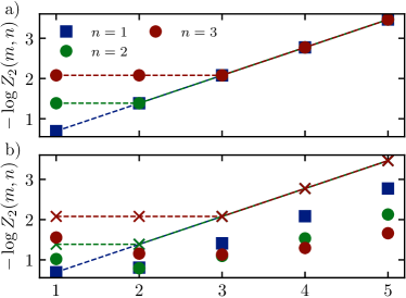
Figure 2: Comparison of the Rényi-2 operator entanglement of the time-evolution operator (solid markers) with theoretical predictions (dashed lines and crosses). (a) $\bar{\mathcal{L}}_{2}$ circuits show excellent agreement with Eq. (25). The gate is chosen randomly from the known set of qubit $\bar{\mathcal{L}}_{2}$ gates (see App. A). (b) A circuit made of gates locally equivalent to those of (a) but without the $\bar{\mathcal{L}}_{2}$ property. Despite the gate having the same operator entanglement, the properties of the global time evolution operator differ drastically. This distinction highlights the importance of the local structure of $\bar{\mathcal{L}}_{k}$ gates.

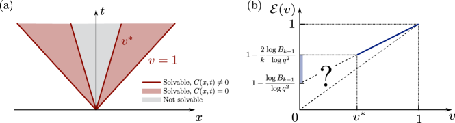
Figure 3: (a) In $\bar{\mathcal{L}}_{k\geq 3}$ circuits the correlations are solvable above a threshold velocity $v_{*}=(k-2)/k$. Inside this range the correlations vanish exactly. Non-vanishing but solvable correlations occur on the boundaries of the solvable region for $\lvert v\rvert=v_{*}$ and $\lvert v\rvert=1$. (b) The ELT is solvable in the same velocity range and takes a linear form there. The partial knowledge of the ELT can be used to infer bounds on the entanglement velocity $v_{E}$ indicated on the vertical axis.

II.1.2 Maximal butterfly velocity and information recovery

The ELT contains two crucial pieces of physical information. First, the butterfly velocity $v_{B}$ is determined by $\mathcal{E}(v_{B})=v_{B}$. For all entangling $\bar{\mathcal{L}}_{2}$ circuits ($B_{1}<q^{2}$) the only solution to this equation is $v_{B}=1$. Therefore, in all entangling $\bar{\mathcal{L}}_{2}$ circuits information spreads at the maximal speed allowed by causality. This shows that dual-unitary circuits are in fact not the only chaotic models with maximal butterfly velocity, as previously conjectured in Ref. [26].

The conclusion that $v_{B}=1$ can also be reached in a more direct manner by relating the operator entanglement to the Hayden-Preskill protocol. This protocol is concerned with the question of recovering quantum information from a small subsystem of a thermodynamically large quantum system following unitary evolution [40]. The information is injected in subsystem $A$ and is supposed to be recovered from $D$ at a later time . Here we consider the setup where the subsystems $A$ and $D$ are connected by a light ray at distance $\ell$. Additionally, we assume that $A$ and $D$ are both composed of a single qudit, resulting in a setup of the form

$$\vbox{\hbox{\includegraphics[height=216.81pt]{figs/hp_hierarchical.png}}}.$$ (32)

As recently discussed in Ref. [42], the fidelity of information recovery is related to the operator purity of the diagonal composition of $\ell-1$ gates as given by

$$B_{\ell-1}\equiv q^{\ell}\,\underbrace{\vbox{\hbox{\includegraphics[width=238.49231pt]{figs/op_purity.png}}}}_{\ell-1}.$$ (33)

While for generic gates this quantity tends to the same value that non-entangling gates take as $\ell\rightarrow\infty$, indicating generic operator spreading with a non-maximal butterfly velocity, the $\bar{\mathcal{L}}_{2}$ property implies that the operator purity remains non-trivial for $\ell\rightarrow\infty$. This signifies that $\bar{\mathcal{L}}_{2}$ circuits transport a finite fraction of information along the light-like direction, directly implying a maximal butterfly velocity. As the entanglement velocity is also determined by the operator entanglement of the gate, this point of view provides a link between the dynamics along the light cone and the local entanglement production. This thought experiment also enables a crucial distinction between dual-unitary and $\bar{\mathcal{L}}_{2}$ circuits: dual-unitary circuits transport the complete amount of information along the light cone, while for $\bar{\mathcal{L}}_{2}$ circuits only a finite fraction of information is transported along the light cone.

II.1.3 Entanglement growth

The second important piece of information is the entanglement velocity as given by $v_{E}=\mathcal{E}(0)$. In $\bar{\mathcal{L}}_{2}$ circuits the entanglement velocity is smaller than $v_{B}$ and it is determined only by the operator entanglement of the gate. As we will discuss in more detail in Sec. V, $\bar{\mathcal{L}}_{2}$ gates have a flat Schmidt spectrum, i.e. all nonzero Schmidt values $\lambda_{i}$ from Eq. (26) are equal. Together with the normalization condition $\sum_{i}\lambda_{i}^{2}=q^{2}$, this result implies that the entanglement velocity can only take a discrete set of possible values for a given local Hilbert space dimension $q$. Fixing the total number of nonzero Schmidt values as the Schmidt rank $\mathcal{R}$, these nonzero Schmidt values necessary equal $\lambda_{i}=q/\sqrt{\mathcal{R}},i=1\dots\mathcal{R}$, resulting in $B_{1}=q^{2}/\mathcal{R}$. Eq. (29) then reduces to

$$v_{E}=\frac{\log\mathcal{R}}{\log q^{2}}\,.$$ (34)

For bipartite unitary gates acting on $\mathbb{C}^{q}\otimes\mathbb{C}^{q}$ all Schmidt ranks from $1$ to $q^{2}$ are possible except for $q=2$ [43, 44]. For qubits the only possible values are $\mathcal{R}=1,2,4$ leading to possible entanglement velocities $v_{E}=0$ (non-entangling), $v_{E}=1$ (dual-unitary), and $v_{E}=1/2$. The latter is realized by CNOT gates, illustrating the general result that bipartite unitaries having Schmidt rank 2 and 3 can be written as controlled unitaries [45, 46].

The form of the ELT in $\bar{\mathcal{L}}_{2}$ circuits is particularly simple as it has no curvature. It is thus extremal in the sense that it takes the maximal values allowed by convexity given $v_{E}$ and $v_{B}$. Interestingly, this piecewise linear form saturates two general bounds on entanglement growth that were conjectured by Mezei and Stanford [47]. It was first remarked in Ref. [48] that such a piecewise linear ELT implies the saturation of these bounds. The first bound, originally formulated in Ref. [49], is

$$S_{A}(t)\leq s_{\mathrm{eq}}\mathrm{vol}(\mathrm{tsunami}(t)),$$ (35)

where $\mathrm{vol}(\mathrm{tsunami}(t))$ is the volume of the region that is causally connected to $A$, called the “entanglement tsunami” [50, 51, 52, 53]. The causal speed can be taken to be $v_{B}$. This bound states that entanglement growth is limited by causality, i.e., entanglement cannot be produced between causally disconnected regions. The second bound concerns the growth rate of the entropy

$$\frac{\mathrm{d}S_{A}(t)}{\mathrm{d}t}\leq v_{E}\lvert\partial A\rvert s_{\mathrm{eq}}.$$ (36)

This bound contains the insight that entanglement is only produced at the boundary between subsystems. These bounds were found to be saturated in certain holographic theories [54]. It is somewhat surprising that this is also the case in unrelated lattice models with finite local Hilbert space dimension. However, we note that $\bar{\mathcal{L}}_{2}$ circuits share a curious feature with the operator spreading picture invoked in Ref. [47] to explain the saturation of the bounds: the entanglement velocity is directly related to the amount of information passed along the light cone. $\bar{\mathcal{L}}_{2}$ circuits provide a natural setting in which this physics is realized.

As most interesting physical consequences of the Mezei-Stanford bounds occur in spatial dimensions $d>1$, where entanglement growth depends on the geometric shape of the bipartition [47], it would be interesting to find higher-dimensional generalizations of $\bar{\mathcal{L}}_{2}$ circuits.

II.2 Connection to temporal entanglement and correlation functions

What lies behind the solvability of the $\bar{\mathcal{L}}_{2}$ circuits? It turns out that the influence matrix (IM) [55, 56, 57], an object that encodes the back action of a system on its local subsystems, is area-law entangled and can be explicitly constructed – taking a simple multi-site product state form. The influence matrix can be generalized to arbitrary time-like surfaces with slope $0\leq v\leq 1$ [58]. Such a generalized IM can then be used to compute dynamical two-point correlations along rays with velocity $v$ in space-time. We focus on influence matrices for correlations at infinite temperature here, which can be be directly related to the ELT. For a quench from an initial state it is not guaranteed that the IM follows the area law, unless the state satisfies a solvability condition (see Ref. [27]).

For $\bar{\mathcal{L}}_{2}$ circuits the IM follows an area law for all $v$. For $v=0$ we can consider, e.g., the right influence matrix

$$\vbox{\hbox{\includegraphics[width=130.08731pt]{figs/influence_lhs.png}}}\,=\,\vbox{\hbox{\includegraphics[width=56.37271pt]{figs/influence_rhs.png}}}.$$ (37)

Here the left-hand side is the definition of the influence matrix, as illustrated for six discrete time steps, and we have applied the hierarchical conditions to reduce the general expression on the left to the final result on the right. Crucially, while the IM on the left generally exhibits volume-law entanglement, the expression on the right can clearly be decomposed in a product of two-site operators and has area-law entanglement. For general $v$ the definition of the IM has a nonzero slope $v$ and a similar decomposition follows using a similar algorithm as in the computation of $Z_{\alpha}$.

The IM can be used to extract the ELT along $v$, as we explain now. Consider $Z_{\alpha}$ for integer $\alpha\geq 2$ and notice that it can be broken up into parts such as

$$\vbox{\hbox{\includegraphics[width=325.215pt]{figs/elt_decomposition.png}}}.$$ (38)

These parts can be identified with tensor products of influence matrices with corresponding slope $v$, as

$$Z_{\alpha}(x,y)=\langle L_{v}\rvert^{\otimes\alpha}\mathcal{S}T_{v}\lvert R_{v}\rangle^{\otimes\alpha},$$ (39)

where $\mathcal{S}$ is a cyclic permutation in replica space and $T_{v}$ is a dual transfer matrix. $\lvert R_{v}\rangle$ and $\langle L_{v}\rvert$ denote right and left IMs, respectively. This decomposition is not unique, but for a coarse grained description only the slope $v$ is relevant. Clearly, if the IM follows an area law the ELT can be computed efficiently. We see that the ELT is solvable if and only if the dynamical two-point correlator is solvable.

The above construction establishes a direct link between the ELT and dynamical correlation functions by showing that both quantities originate from the same fundamental object, the infinite temperature IM. It remains an interesting question if this link can lead to further insight on the connections between these quantities. In the case of $\bar{\mathcal{L}}_{2}$ circuits the IM not only follows an area law, it takes the form of a product state of, in general, dimers and monomers. This property lies behind the vanishing of correlation functions, since – loosely speaking – the lack of temporal entanglement between sites at the initial and final time leads the correlation to vanish. (This argument fails only when the correlation is produced by the dual-transfer matrix carrying the operators, as is the case at $v=0$ and $v=\pm 1$.) On the other hand, the factorization of the IM also leads to the linear form of the ELT.

The area-law IM also gives some insight into the operator spreading picture of correlations. In the language of Ref. [48] it implies that there are no operators contracting to a point for $0<\lvert v\rvert<1$ and that the operator trajectories contributing to the correlator for $v=0,\pm 1$ are “thin” (see Ref. [48] for details).

II.3 Higher levels of the hierarchy

The ideas developed in the above sections can be applied, with minor modifications, to higher levels of the hierarchy. However, there is a crucial difference. While for $\bar{\mathcal{L}}_{2}$ circuits the ELT and correlations are solvable in the full spacetime, for higher levels the solvability is constrained to a range of velocities $v_{*}\leq\lvert v\rvert\leq 1$, as schematically depicted in Fig. 3. In this range, the ELT is linear and the correlations vanish exactly (apart from the edge rays $\lvert v\rvert=v_{*}$ and $\lvert v\rvert=1$), but outside of this range their evaluation is in general exponentially hard. We show that generally $\bar{\mathcal{L}}_{k}$ circuits have maximal butterfly velocity and we provide bounds on the entanglement velocity.

Consider now an $\bar{\mathcal{L}}_{k}$ circuit with $k>2$. The ELT is computed using the same algorithm as outlined above. However, the diagram only factorizes if its width and height satisfy the inequality

$$m\geq(k-1)n\iff v\geq v_{*}\equiv\frac{k-2}{k}.$$ (40)

If this inequality is met we find

$$\mathcal{E}(v)=1-(1-\lvert v\rvert)\frac{\log B_{k-1}}{\log q^{2}},\quad\lvert v\rvert\geq v_{*}.$$ (41)

We can again conclude that for all levels of the hierarchy the butterfly velocity is maximal, $v_{B}=1$, unless $B_{k-1}=q^{2}$ in which the gates are nonentangling. As $\mathcal{E}(v)$ is inaccessible for $v=0$ we cannot compute the entanglement velocity $v_{E}$ exactly. However, convexity of the ELT implies a lower bound on $v_{E}$

$$v_{E}\geq 1-\frac{\log B_{k-1}}{\log q^{2}},\quad U\in\bar{\mathcal{L}}_{k}.$$ (42)

Under the further assumption that $\mathcal{E}^{\prime}(v)\geq 0$ for all $v>0$, i.e., that $\mathcal{E}(v)$ is monotonically increasing, we also obtain an upper bound

$$v_{E}\leq\mathcal{E}(v_{*})=1-\frac{2}{k}\frac{\log B_{k-1}}{\log q^{2}},\quad U\in\bar{\mathcal{L}}_{k}.$$ (43)

This assumption holds in all parity symmetric unitary circuits, where $\mathcal{E}(-v)=\mathcal{E}(v)$, and thus $v=0$ is always a minimum. We expect this assumption to extend to all unitary circuits. It is known to be violated in quantum cellular automata with a finite topological index, where it is associated to a background entanglement current [59]. The bounds are indicated in Fig. 3(b).

The same arguments as above lead to the conclusion that the infinite-temperature IM factorizes for $v_{*}\leq\lvert v\rvert\leq 1$. The correlations thus vanish identically in the range $v_{*}<\lvert v\rvert<1$, and they are solvable but non-trivial for $\lvert v\rvert=v_{*}$ and $\lvert v\rvert=1$.

III Operator growth

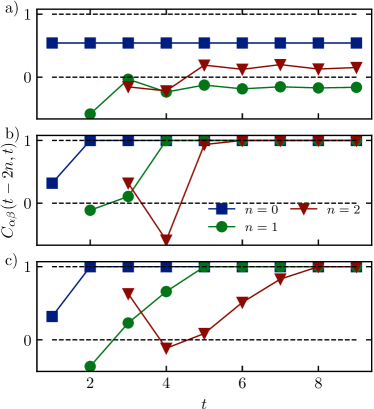
Figure 4: OTOC in qubit $\bar{\mathcal{L}}_{k}$ circuits for randomly selected gates of the given parametrizations. (a) In $\bar{\mathcal{L}}_{2}$ circuits the OTOC does not relax to the trivial value $C=1$, indicating $v_{B}=1$. (b) In the class of $\bar{\mathcal{L}}_{3}$ circuits defined by Eq. (108) the OTOC relaxes to the trivial value exactly for $x\geq 2$. This indicates $v_{B}=0$. (c) Dressing one leg of the gate used in (b) changes its dynamical properties drastically. Now, the OTOC relaxes exactly for $x=(t+4)/3$ indicating $v_{B}=1/3$.

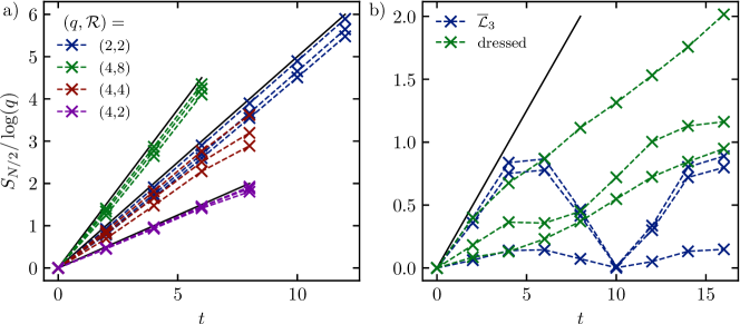
Figure 5: Growth of the half-chain entanglement entropy from random translationally invariant product states. The numerics are performed on chains of $N=24$ qubits and $N=12$ ququads, respectively. (a) The possible values of $v_{E}$ in $\bar{\mathcal{L}}_{2}$ circuits with $q=2$ and $q=4$ are illustrated. The qubit $\bar{\mathcal{L}}_{2}$ gate is randomly selected from the known parametrization. The ququad gates used are: Eq. (63) for $\mathcal{R}=2$, Eq. (65) for $\mathcal{R}=4$, and Eq. (101) for $\mathcal{R}=8$. The solid lines are guides to the eye. (b) An $\bar{\mathcal{L}}_{3}$ gate randomly selected from the known parametrization shows saturation of the entanglement followed by oscillations indicating non-ergodicity. Upon dressing one leg with a randomly selected generic unitary entanglement growth is observed, with a rate satisfying the upper bound $v_{E}\leq 1/3$ imposed by EMT.

As was shown in section II, EMT predicts that operators in $\bar{\mathcal{L}}_{k}$ circuits grow at maximal speed, and that due to the absence of curvature of the ELT there is no diffusive broadening of the operator front. Independently, an argument for maximal operator spreading based on certain quantum-information theoretic properties of $\bar{\mathcal{L}}_{k}$ gates was given. In this section we substantiate these results with more traditional calculations of the OTOC.

Given a basis of orthonormal local operators $\{\sigma_{\alpha},\alpha=0,\ldots,q^{2}-1\}$ satisfying $\operatorname{tr}[\sigma_{\alpha}\sigma_{\beta}]=q\delta_{\alpha\beta}$, $\operatorname{tr}[\sigma_{\alpha}]=\delta_{\alpha 0}$, the OTOC is defined as

$$C_{\alpha\beta}(x,t) =\langle\sigma_{\alpha}(0,t)\sigma_{\beta}(x,0)\sigma_{\alpha}(0,t)\sigma_{\beta}(x,0)\rangle.$$ (44)

Here $\sigma_{\alpha}(0,t)=U(t)\sigma_{\alpha}(x)U(t)^{\dagger}$ and $\sigma_{\alpha}(x)$ acts nontrivially as $\sigma_{\alpha}$ on site $x$ and as the identity everywhere else. The OTOC can again be represented as a tensor network (see Ref. [26]):

$$C_{\alpha\beta}(x,t)=q^{m+n}\,\vbox{\hbox{\includegraphics[width=251.50038pt]{figs/otoc.png}}}$$ (45)

with light-cone coordinates

$$n=\frac{t-x+2}{2},\,\, m=\frac{t+x}{2},\qquad t-x\in 2\mathbb{Z},$$ (46a)

$$n=\frac{t-x+1}{2},\,\, m=\frac{t+x+1}{2},\,\, t-x\in 2\mathbb{Z}+1.$$ (46b)

In the limit $t+x\rightarrow\infty$ the problem of its evaluation reduces to the determination of the leading eigenspace of the light-cone transfer matrix (LCTM) [25, 26]

$$T_{n}=\frac{1}{q}\,\underbrace{\vbox{\hbox{\includegraphics[height=25.29604pt]{figs/transfer_mat_rotated.png}}}}_{n}\,.$$ (47)

In generic unitary circuits, there is a unique leading eigenvector determined purely by unitarity. The absence of further leading eigenvectors reflects a non-maximal butterfly velocity, and an analysis of the subleading eigenvectors is needed to determine the behavior of the OTOC [38, 60]. On the other hand, if the leading eigenspace is degenerate the butterfly velocity is maximal since it leads to a nontrivial OTOC along the light ray $|x|=t$, and the asymptotic profile of the OTOC is determined by the projection of the boundaries of the tensor network on the leading eigenspace. This scenario occurs in dual-unitary circuits, where additional leading eigenvectors can be determined from dual-unitarity, resulting in a set of leading eigenvectors known as a “maximally chaotic subspace” [25, 26].

In $\bar{\mathcal{L}}_{k}$ circuits a set of leading eigenvectors of the LCTM can be constructed analytically, generalizing the maximally chaotic subspace of dual-unitary circuits. Absent any further symmetries we expect this set to be exhaustive. There are however two key differences to DUCs: (i) the left and right leading eigenstates are not the transposed of each other, (ii) the leading eigenstates are in general highly entangled. The latter point implies that even though the leading eigenstates can be constructed, the OTOC cannot be computed exactly beyond small values of $t-x$, as the computation of the overlap with the boundary conditions is exponentially hard.

First, we show how to construct the non-trivial leading eigenvectors for the case of $\bar{\mathcal{L}}_{2}$ circuits. It is easy to check that the staircase vector $\lvert s_{n})$ (shown here for $n=1$ and $n=2$)

$$\lvert s_{1})=\vbox{\hbox{\includegraphics[width=65.04034pt]{figs/staircase1.png}}},\quad\lvert s_{2})=\vbox{\hbox{\includegraphics[width=108.405pt]{figs/staircase2.png}}}.$$ (48)

is a leading eigenvector of the LCTM of width $n$. The remaining leading eigenvectors can be obtained from smaller staircases by forming a tensor product with the trivial leading eigenvector, e.g.,

$$\lvert\Box_{n-1}s_{1})=\,\vbox{\hbox{\includegraphics[width=173.44534pt]{figs/padded_staircase.png}}}.$$ (49)

That this is an eigenvector can be directly checked only using unitarity. This construction provides in total $n+1$ leading eigenvectors, as in the dual-unitary case. The left eigenvectors are constructed in an analogous manner

$$(\tilde{s}_{1}\rvert=\vbox{\hbox{\includegraphics[width=65.04034pt]{figs/left_staircase_1.png}}},\quad(\tilde{s}_{2}\rvert=\vbox{\hbox{\includegraphics[width=108.405pt]{figs/left_staircase_2.png}}}.$$ (50)

Note that the right and left eigenvectors are not the mutual transposed of each other.

To construct the projector on the leading eigenspace the overlap of the eigenvectors is needed. We denote $\lvert r_{k}):=\lvert\Box_{n-k}s_{k})$ and $(\ell_{k}\rvert:=(\tilde{s}_{k}\circ_{n-k}\rvert$. As is shown in Appendix B the overlap matrix (for a channel of width $n$) takes the general form

$$(\ell_{i}|r_{j})=\frac{1}{q^{n}}\begin{pmatrix}1&1&\ldots&&1\\ 1&&&1&b_{1}\\ \vdots&&1&b_{1}&b_{1}^{2}\\ \vdots&\iddots&\iddots&\iddots&\vdots\\ 1&b_{1}&b_{1}^{2}&\ldots&b_{1}^{n}\end{pmatrix},$$ (51)

where $b_{1}:=B_{1}/q^{2}$. This matrix can be identified as a Hankel matrix. We see immediately that it becomes rank deficient if and only if $b_{1}=1$ and hence $B_{1}=q^{2}$, i.e., only for non-entangling gates. In this case the staircase vectors are not linearly independent and thus do not provide any additional leading eigenvectors beyond the trivial one.

The last missing ingredient for the calculation of the asymptotic profile of the OTOC is the overlap with the boundary conditions. Unfortunately, the overlaps between the staircase vectors and the boundary conditions cannot be simplified to an efficiently computable form. Generically, the staircase vectors are volume-law entangled, in contrast to dual-unitary circuits, where they reduce to product states.

To gain information about the behavior of operator dynamics deep inside the light cone, we instead focus on the tripartite information [61, 62, 63], a quantity that is amenable to exact calculation in ergodic $\bar{\mathcal{L}}_{2}$ circuits. Details of the calculation are presented in App. C. We find

$$I^{(3)}(x,t)\approx(t-x)\log(b_{1}),\quad t+x\gg 1.$$ (52)

For $x<t$ the tripartite information is negative and large, indicating scrambling. Moreover, the front defined by $x=t$ is sharp, it does not broaden diffusively.

For the higher levels of the hierarchy the construction is analogous, merely the height of the steps changes,

$$\lvert s_{1})=\vbox{\hbox{\includegraphics[width=65.04034pt]{figs/staircase_l3_1.png}}},\quad\lvert s_{2})=\vbox{\hbox{\includegraphics[width=108.405pt]{figs/staircase_l3_2.png}}}.$$ (53)

Analysis of the overlaps shows that the Hankel matrix structure is preserved and the condition for linear dependence becomes $B_{k-1}=q^{2}$ for gates from $\bar{\mathcal{L}}_{k}$. This implies that for $k\geq 3$ there can be $\bar{\mathcal{L}}_{k}$ circuits which are not product gates, but still have $v_{B}<1$. In this case, for ergodic circuits the ELT gives the upper bound $v_{B}\leq v_{*}$. The $\bar{\mathcal{L}}_{3}$ gates known so far all have the property $B_{2}=q^{2}$, thus a non-maximal butterfly velocity is expected. The parametrization of qubit $\bar{\mathcal{L}}_{3}$ gates is reviewed in App. A. For these circuits, our numerical results are consistent with a vanishing butterfly velocity, $v_{B}=0$, indicating strong non-ergodicity [Fig. 4(b)]. In fact, it can be shown that they display localized behavior by a slight modification of the argument presented in Ref. [64]. Ergodic gates retaining some of the solvability can be constructed starting from this class of gates by dressing only one of the legs with a generic local unitary transformation. This preserves the $\bar{\mathcal{L}}_{3}$ property along one of the light-cone directions but breaks it along the other. As a result the solvability is preserved only for positive (negative) velocities. Along the remaining solvable direction the $\bar{\mathcal{L}}_{3}$ structure enforces the bound $v_{B}\leq 1/3$. Our numerical results are consistent with $v_{B}=1/3$ [Fig. 4(c)]. Curiously, this class of gates seem to have a non-zero butterfly velocity even though all subleading eigenvalues of the LCTM vanish, contrary to expectations. This is possible if the largest Jordan block grows fast enough with the width of the LCTM. Details on this mechanism are provided in App. D.

IV Entanglement growth

In this section we check the prediction of the entanglement velocity provided by EMT. We present numerical results supporting the EMT picture for entanglement growth in $\bar{\mathcal{L}}_{2}$ and $\bar{\mathcal{L}}_{3}$ circuits in Fig. 5. We consider random translation invariant product states as initial states. Analytical calculations from special solvable states supporting the EMT picture were presented in Ref. [36].

In $\bar{\mathcal{L}}_{2}$ circuits, for a given local Hilbert space dimension only a discrete set of entanglement velocities, corresponding to allowed Schmidt ranks $\mathcal{R}$ are possible. E.g., for qubits the only non-trivial possibility is $v_{E}=1/2$ ($\mathcal{R}=2$). For ququads ($q=4$) the possible values are $v_{E}=1/4$ ($\mathcal{R}=2$), $v_{E}=1/2$ ($\mathcal{R}=4$), and $v_{E}=3/4$ ($\mathcal{R}=8$). The gates constructed in Sec. V provide the first examples of $\bar{\mathcal{L}}_{2}$ gates falling into the classes $(q,\mathcal{R})=(4,2)$ and $(q,\mathcal{R})=(4,8)$. Unfortunately they are non-ergodic, but it is likely that locally equivalent ergodic gates exist. Despite their non-ergodicity, the entanglement growth from generic states is consistent with the predictions of ELT [Fig. 5(a)]. This result reflects that the operator entanglement of the time-evolution operator encodes generic aspects of entanglement growth.

The strong non-ergodicity of the qubit $\bar{\mathcal{L}}_{3}$ circuits is reflected in the rapid saturation of the half-chain entanglement to an $\mathcal{O}(1)$ value. On the other hand, the one-sided dressing induces a finite entanglement velocity consistent with the bound $v_{E}<1/3$ [Fig. 5(b)].

V Existence and construction of $\bar{\mathcal{L}}_{2}$ gates

In this section we detail some of the properties of the Schmidt spectrum (26) of $\bar{\mathcal{L}}_{2}$ gates and use these as a guiding principle to obtain construction of $\bar{\mathcal{L}}_{2}$ gates for systems with arbitrary dimension of the local Hilbert space. In the two-qubit case an exhaustive parametrization exists of both dual-unitary gates and $\bar{\mathcal{L}}_{2}$ gates, but going to larger Hilbert spaces can allow for a phenomenology inaccessible in qubits (see e.g. Ref. [23] for dual-unitary gates). Here we discuss new constructions of $\bar{\mathcal{L}}_{2}$ for higher local Hilbert space dimensions by taking insights from several existing constructions of dual-unitary gates, which will allow us to e.g. generalize the CNOT construction for qubits to larger Hilbert spaces in various ways. These results are meant to be an initial exploration, showing how different Schmidt ranks and hence different entanglement velocities can be obtained, and will be expanded on in later works.

The $\bar{\mathcal{L}}_{2}$ conditions strongly restrict the Schmidt spectrum: all such gates have a non-maximal Schmidt rank, i.e. $\mathcal{R}<q^{2}$, and the Schmidt spectrum is flat, i.e. all nonzero Schmidt values are equal.

The first property can be directly shown by noting that a maximal Schmidt rank implies that the inverse of $\tilde{U}$ exists, where $\tilde{U}$ is the space-time dual of $U$ defined as $\tilde{U}_{ab,cd}=U_{ac,bd}$. Representing this (folded) inverse as a green tensor, we can contract the hierarchical condition (11) with this inverse acting on the two lowest Hilbert spaces in the diagram to obtain

$$\vbox{\hbox{\includegraphics[height=69.38078pt]{figs/full_rank_deriv_2.png}}}\,=\,\vbox{\hbox{\includegraphics[height=69.38078pt]{figs/full_rank_deriv_1.png}}}\,=\,\vbox{\hbox{\includegraphics[height=69.38078pt]{figs/full_rank_deriv_3.png}}}\,=\,\vbox{\hbox{\includegraphics[height=69.38078pt]{figs/full_rank_deriv_4.png}}}.$$ (54)

The above equation factorizes and is satisfied if and only if $U$ is dual unitary. Therefore, any unitary gate $U$ on $\mathbb{C}^{q}\otimes\mathbb{C}^{q}$ with full Schmidt rank satisfies the $\mathcal{L}_{2}$ conditions if and only if it is a dual unitary. As such, all $\bar{\mathcal{L}}_{2}$ gates have Schmidt rank less than $q^{2}$.

The flatness of the Schmidt spectrum was proven in Ref. [36]. A defining property of dual-unitary gates is that these have a flat Schmidt spectrum with maximal rank i.e., $\lambda_{i}=1$ for all $i=1\dots q^{2}$. For hierarchical $\bar{\mathcal{L}}_{2}$ gates we conversely find that these gates satisfy $\lambda_{i}=q/\sqrt{\mathcal{R}}$ for all $i=1,\dots\mathcal{R}<q^{2}$, with a nonzero amount of vanishing Schmidt values. The maximal rank $\mathcal{R}=q^{2}$ corresponds to dual-unitaries and the opposite limit of $\mathcal{R}=1$ corresponds to unentangled products of one-site unitaries. While this is a necessary condition for $\bar{\mathcal{L}}_{2}$, it turns out to not be a sufficient condition. In the remainder of this section we will present systematic constructions of gates with a flat Schmidt spectrum with non-maximal rank and identify the gates that satisfy the $\bar{\mathcal{L}}_{2}$ condition.

V.1 $\bar{\mathcal{L}}_{2}$ gates with Schmidt rank $q$

Consider a controlled unitary gate on $\mathbb{C}^{q}\otimes\mathbb{C}^{q}$ given by

$$U=\sum_{i=1}^{q}\lvert i\rangle\langle i\rvert\otimes u_{i},$$ (55)

where $u_{i}\in\mathbb{U}(q)$. By choosing the unitary gates to satisfy $\operatorname{tr}(u_{i}^{\dagger}u_{j})=\delta_{ij}$ it can be directly checked that these gates have a flat Schmidt spectrum with rank $\mathcal{R}$. The CNOT gate can be extended to arbitrary $q$ by choosing $u_{i}=X^{i}$, where $X\lvert k\rangle=\lvert k\oplus 1\rangle$ is the shift operator ($\oplus$ denotes addition $\bmod\,q$). The resulting generalized CNOT gates are well known and given by

$$U_{\text{CNOT}}=\sum_{i=1}^{q}\,\lvert i\rangle\langle i\rvert\otimes X^{i-1}.$$ (56)

These have Schmidt rank $\mathcal{R}=q$ and satisfy the $\bar{\mathcal{L}}_{2}$ properties for arbitrary $q$, as also observed in Ref. [27]. This result can be checked by direct calculation. Furthermore, for all such controlled unitary gates the $\bar{\mathcal{L}}_{2}$ property is invariant under local multiplication with enphased permutation gates. For a possible permutation $P$ of the $i$ basis elements and a set of phases $\phi_{i},i=1\dots 1$ we can define an enphased permutation gate $u_{P}$ as

$$\langle a\rvert u_{P}\lvert b\rangle=e^{i\phi_{a}}\delta_{b,P(a)}.$$ (57)

A set of $\bar{\mathcal{L}}_{2}$ gates can then be obtained as

$$(u_{P_{1}}\otimes u_{P_{2}})U_{\text{CNOT}},$$ (58)

where both the two permutations $P_{1}$ and $P_{2}$ and the two corresponding sets of phases can be chosen independently. That this parametrization returns an $\bar{\mathcal{L}}_{2}$ gate can be understood by explicitly rewriting the hierarchical conditions (11) for a controlled gate. Controlled gates of the form (55) can be graphically represented as

$$\vbox{\hbox{\includegraphics[width=130.08731pt]{figs/CNOT}}}\,.$$ (59)

The hierarchical condition (11) reads

$$\vbox{\hbox{\includegraphics[width=195.12767pt]{figs/CNOT_1}}}\,\,,$$ (60)

where the folded gates now correspond to $U\otimes U^{*}$ (and hence $\alpha=1$). It can be easily checked that a sufficient condition for this equation to hold is that

$$\vbox{\hbox{\includegraphics[width=95.39693pt]{figs/CNOT_2}}}\,,\qquad\forall j=1\dots q\,,$$ (61)

where $(j,j)$ denotes the folded version of $\lvert j\rangle\langle j\rvert$. Expressing the folded diagram algebraically, this equation corresponds to

$$\sum_{i=1}^{q}u_{i}\lvert j\rangle\langle j\rvert u_{i}^{\dagger}=\mathbbm{1},\qquad\forall j=1\dots q.$$ (62)

This equation is satisfied whenever $\{u_{i}\lvert j\rangle,i=1\dots q\}$ forms a complete basis for each choice of $j$, as can be directly checked to be the case for the above construction.

The CNOT example for $q=2$ can be extended to higher $q$ in a different way for even local Hilbert space dimension by consider the controlled $X$ gate as given by

$$CX=\sum_{i=1}^{q}\lvert i\rangle\langle i\rvert\otimes W_{i},$$ (63)

where $W_{i}=\mathbbm{1}_{q}$ for $i\bmod 2=0$ and $W_{i}=X$ otherwise. This permutation gate now has Schmidt rank $\mathcal{R}=2$ with $\lambda_{0}=\lambda_{1}=q/\sqrt{2}$ and again satisfies the $\bar{\mathcal{L}}_{2}$ constraints. This construction can again be generalized by considering two permutations $P$ and $Q$, where $P$ preserves the parity, $P(i)=i\bmod 2$ and $Q$ switches the parity, $Q(i)=i+1\bmod 2$. The resulting gates can again be enphased, where we define $U_{a,b}=e^{i\phi_{a}}\delta_{b,P(a)}$ and $V_{a,b}=e^{i\psi_{a}}\delta_{b,Q(a)}$, resulting in a $\bar{\mathcal{L}}_{2}$ gate

$$U=\sum_{i=1}^{q}\lvert i\rangle\langle i\rvert\otimes W,$$ (64)

where $W_{i}=U$ for $i\bmod 2=0$ and $W_{i}=V$ otherwise.

We note that all $\bar{\mathcal{L}}_{2}$ gates in local dimension $q=2$ are T-dual and satisfy Eq. (16). For local dimensions $q\geq 4$, there exist $\bar{\mathcal{L}}_{2}$ gates that are not T-dual. For example, in local dimension $q=4$ consider the following permutation gate satisfies the $\bar{\mathcal{L}}_{2}$ condition:

$$\mathcal{P}=(CX)S(CX)S,$$ (65)

where $CX$ is given by Eq. (63) and $S$ is the SWAP gate. The resulting permutation gate $\mathcal{P}$ has Schmidt rank $\mathcal{R}=4$ with $\lambda_{0}=\cdots=\lambda_{3}=2$, but direct calculation shows that it is not T-dual.

V.2 $\bar{\mathcal{L}}_{2}$ gates with Schmidt rank two

In the previous subsection, we explicitly showed how $\bar{\mathcal{L}}_{2}$ gates with Schmidt rank two can be systematically constructed for an even local Hilbert space dimension. It is a natural question to ask if this construction can be extended to odd local Hilbert space dimension. Here we will show that unitary gates with flat Schmidt spectrum and Schmidt rank two do not exist for odd local Hilbert space dimensions. Consequently, $\bar{\mathcal{L}}_{2}$ gates with Schmidt rank two do not exist in this case.

The proof of the above result relies on the fact that every bipartite unitary gate with $\mathcal{R}=2$ is locally equivalent to a controlled unitary [45]. Local equivalence does not change the Schmidt spectrum, so we can consider the Schmidt spectrum of

$$U=\sum_{i=1}^{q}\lvert i\rangle\langle i\rvert\otimes u_{i},$$ (66)

where $u_{i}\in\mathbb{U}(q)$. For Schmidt rank two there are only two linearly independent $u_{i}$’s and, without loss of generality, we assume there are only two distinct blocks. Among these two distinct blocks one of the blocks can always be chosen to be the identity matrix by a local change of basis. As we are interested in unitary gates with a flat Schmidt spectrum this implies that the other (orthonormal) unitary must be traceless. Therefore, we can express the above controlled unitary as

$$U=\left(\sum_{j=1}^{q_{1}}\lvert j\rangle\langle j\rvert\right)\otimes\mathbbm{1}_{q}+\left(\mathbbm{1}_{q}-\sum_{j=1}^{q_{1}}\lvert j\rangle\langle j\rvert\right)\otimes u,\quad 1<q_{1}<q,$$ (67)

where we have separated the terms based on whether the action on second qudit is trivial or not. From the above equation we write the Schmidt decomposition as follows,

$$U=\sqrt{q\,q_{1}}\,\left(M\otimes\frac{\mathbbm{1}_{q}}{\sqrt{q}}\right)+\sqrt{q\,(q-q_{1})}\,\left(M^{\perp}\otimes\frac{u}{\sqrt{q}}\right),$$ (68)

where

$$M=\frac{1}{\sqrt{q_{1}}}\sum_{j=1}^{q_{1}}\lvert j\rangle\langle j\rvert,\qquad M^{\perp}=\frac{\mathbbm{1}_{q}-\sqrt{q_{1}}\,M}{\sqrt{q-q_{1}}},$$ (69)

are properly normalized. The Schmidt coefficients can be read off as $\lambda_{1}=\sqrt{q\,(q-q_{1})}$ and $\lambda_{2}=\sqrt{q\,q_{1}}$. The condition for flat Schmidt spectrum $\lambda_{1}=\lambda_{2}$ then leads to

$$\sqrt{q\,(q-q_{1})} =\sqrt{q\,q_{1}}\quad\implies\quad q_{1}=\frac{q}{2}.$$ (70)

Therefore, $\lambda_{1}=\lambda_{2}$ is possible only when $q$ is divisible by 2 since $q_{1}$ is an integer dimension.

V.3 $\bar{\mathcal{L}}_{2}$ gates with larger Schmidt ranks in non-prime dimensions

Here we discuss the construction of $\bar{\mathcal{L}}_{2}$ gates using block-diagonal unitaries for non-prime local dimension; $q=p_{1}p_{2}$, where $p_{1}$, $p_{2}$ are prime, such that $\mathbb{C}^{q}\otimes\mathbb{C}^{q}\sim\mathbb{C}^{p_{1}}\otimes\mathbb{C}^{qp_{2}}\sim\mathbb{C}^{p_{2}}\otimes\mathbb{C}^{qp_{1}}$. Consider a block-diagonal unitary on $\mathbb{C}^{p_{1}}\otimes\mathbb{C}^{qp_{2}}$ constructed out of a set of $p_{1}$ one-site unitary matrices $V_{k}\in\mathbb{U}(qp_{2})$ as

$$U =\sum_{k=1}^{p_{1}}\lvert k\rangle\langle k\rvert\otimes V_{k}=\left(\begin{array}[]{c|c|c|c}V_{1}&\cdots&\cdots&\cdots\\ \hline\cr\cdots&V_{2}&\cdots&\cdots\\ \hline\cr\cdots&\cdots&\cdots&\cdots\\ \hline\cr\cdots&\cdots&\cdots&V_{p_{1}}\\ \end{array}\right).$$ (75)

As we are interested in unitary matrices for which the Schmidt spectrum is flat, this requires that the unitary matrices $V_{k}$ acting on $\mathbb{C}^{p_{2}}\otimes\mathbb{C}^{q}$ are maximally entangled. Therefore, the construction of block-diagonal unitaries of the form given in Eq. (75) which have a flat Schmidt spectrum reduces to finding maximally entangled unitary gates in $\mathbb{C}^{p_{2}}\otimes\mathbb{C}^{q}$. Similarly, the construction of block-diagonal unitary gates on $\mathbb{C}^{q_{2}}\otimes\mathbb{C}^{p_{1}q}$ with flat Schmidt spectrum reduces to finding maximally entangled unitary gates in $\mathbb{C}^{p_{1}}\otimes\mathbb{C}^{q}$.

A well-known example of a maximally entangled operator on $\mathbb{C}^{q_{1}}\otimes\mathbb{C}^{q_{2}}$ is the quantum Fourier transform or Fourier gate [65]. The Fourier gate $F_{q_{1}\times q_{2}}:\mathbb{C}^{q_{1}}\otimes\mathbb{C}^{q_{2}}\mapsto\mathbb{C}^{q_{1}}\otimes\mathbb{C}^{q_{2}}$ is defined as

$$\langle m,n\rvert F_{q_{1}\times q_{2}}\lvert m^{\prime},n^{\prime}\rangle=\frac{1}{\sqrt{q_{1}q_{2}}}\omega^{((m-1)q_{2}+n-1)((m^{\prime}-1)q_{2}+n^{\prime}-1)},$$ (76)

where $\omega=\exp({2\pi i}/{(q_{1}q_{2})})$ and $m,m^{\prime}$ take values from 1 to $q_{1}$ and $n,n^{\prime}$ take values from 1 to $q_{2}$. If $q_{1}\leq q_{2}$, then $F_{q_{1}\times q_{2}}$ is maximally entangled if $q_{1}$ divides $q_{2}$ i.e., $q_{2}\mod q_{1}=0$ [65]. Using maximally entangled unitaries such as the Fourier gate defined above, we illustrate the above construction of $\bar{\mathcal{L}}_{2}$ gates in local dimension $q=4$ below.

V.3.1 Illustration of the construction for $q=4$

For local dimension $q=4=2\times 2$, consider the following unitary gate

$$U =\sum_{k=1}^{2}\lvert k\rangle\langle k\rvert\otimes F_{2\times 4}=\left(\begin{array}[]{c|c}F_{2\times 4}&{\bf 0}\\ \hline\cr{\bf 0}&F_{2\times 4}\end{array}\right).$$ (79)

As $F_{2\times 4}$ is a maximally entangled unitary on $\mathbb{C}^{2}\otimes\mathbb{C}^{4}$, it has four orthonormal $4\times 4$ blocks. Therefore the above unitary has Schmidt rank $\mathcal{R}=4$ and has a flat Schmidt spectrum. It can again be checked by direct calculation that this presents an $\bar{\mathcal{L}}_{2}$ gate. One can obtain an $\bar{\mathcal{L}}_{2}$ gate with Schmidt rank eight by permuting the rows and columns of one of the $F_{2\times 3}$ blocks appearing in above equation in such a way that the resultant $8\times 8$ unitary matrix has orthonormal blocks with that of $F_{2\times 4}$. One of the examples is the following gate

$$U^{\prime}=\left(\begin{array}[]{c|c}F_{2\times 4}&{\bf 0}\\ \hline\cr{\bf 0}&F_{2\times 4}^{\prime}\end{array}\right),$$ (80)

where $F_{2\times 4}^{\prime}=X^{2}F_{2\times 4}X^{2}$ and $X$ is the shift operator on $\mathbb{C}^{8}$; $X\lvert k\rangle=\lvert(k+1)\bmod 8\rangle$. The unitary $U^{\prime}$ has Schmidt rank $\mathcal{R}=8$ with flat Schmidt spectrum, $\lambda_{1}=\lambda_{2}=\cdots=\lambda_{8}=\sqrt{2}$, and also satisfies the $\bar{\mathcal{L}}_{2}$ conditions.

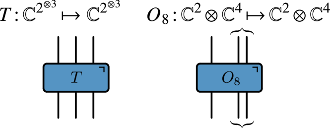
Figure 6: A three-qubit perfect tensor $T$ with three input and three output legs is reshaped into a tensor $O_{8}$ which has two input and two output legs, where two legs of $T$ can be combined to return a composite Hilbert space with dimension $4$.

Another way to obtain maximally entangled unitaries on $\mathbb{C}^{2}\otimes\mathbb{C}^{4}$ is using the six-qubit perfect tensor. By definition, a perfect tensor [66] defines an isometry under arbitrary partitioning of its indices into two disjoint sets. The six-qubit perfect tensor defines a special pure state of six qubits that has maximal entanglement with respect to all bipartitions [67, 66]. Such states, also known as absolutely maximally entangled (AME) states, have useful applications in quantum error correction, quantum teleportation, and quantum secret sharing [68]. A six-qubit AME state can be obtained by the superposition of the logical states of the well-known five-qubit error correcting code [69]. A convenient representation of the six-qubit perfect tensor exists in terms of a real Hadamard matrix of size 8 given by [67]

$$O_{8}=\frac{1}{\sqrt{8}}\left(\begin{array}[]{cccc|cccc}-&-&-&+&-&+&+&+\\ -&-&-&+&+&-&-&-\\ -&-&+&-&-&+&-&-\\ +&+&-&+&-&+&-&-\\ \hline\cr-&+&-&-&-&-&+&-\\ +&-&+&+&-&-&+&-\\ +&-&-&-&+&+&+&-\\ +&-&-&-&-&-&-&+\end{array}\right),$$ (81)

where $+$ denotes $+1$ and $-$ denotes $-1$. The above representation is given in the three-qubit computational basis, e.g. $\langle 000\rvert O_{8}\lvert 000\rangle=-1/\sqrt{8},\langle 000\rvert O_{8}\lvert 001\rangle=-1/\sqrt{8},\cdots,\langle 111\rvert O_{8}\lvert 111\rangle=1/\sqrt{8}$.

We now consider the mapping $O_{8}:\mathbb{C}^{2}\otimes\mathbb{C}^{4}\mapsto\mathbb{C}^{2}\otimes\mathbb{C}^{4}$, as indicated by partitioning the $O_{8}$ matrix into $4\times 4$ blocks. This is also illustrated in Fig. 6 in which we group together a pair of both input and output legs of a six-qubit perfect tensor resulting into a bipartite unitary on $\mathbb{C}^{2}\otimes\mathbb{C}^{4}$. One can easily check that the four $4\times 4$ blocks in $O_{8}$ are orthonormal and its Schmidt spectrum is flat; $\lambda_{1}=\lambda_{3}=\lambda_{3}=\lambda_{4}=\sqrt{2}$.

In order to obtain $\bar{\mathcal{L}}_{2}$ gates using the $O_{8}$ matrix, we consider the block-diagonal unitary $U\in\mathbb{U}(16)$ given by

$$U =O_{8}\oplus O_{8}=\frac{1}{\sqrt{8}}\left(\begin{array}[]{cccc|cccc|cccc|cccc}-&-&-&+&-&+&+&+&.&.&.&.&.&.&.&.\\ -&-&-&+&+&-&-&-&.&.&.&.&.&.&.&.\\ -&-&+&-&-&+&-&-&.&.&.&.&.&.&.&.\\ +&+&-&+&-&+&-&-&.&.&.&.&.&.&.&.\\ \hline\cr-&+&-&-&-&-&+&-&.&.&.&.&.&.&.&.\\ +&-&+&+&-&-&+&-&.&.&.&.&.&.&.&.\\ +&-&-&-&+&+&+&-&.&.&.&.&.&.&.&.\\ +&-&-&-&-&-&-&+&.&.&.&.&.&.&.&.\\ \hline\cr.&.&.&.&.&.&.&.&-&-&-&+&-&+&+&+\\ .&.&.&.&.&.&.&.&-&-&-&+&+&-&-&-\\ .&.&.&.&.&.&.&.&-&-&+&-&-&+&-&-\\ .&.&.&.&.&.&.&.&+&+&-&+&-&+&-&-\\ \hline\cr.&.&.&.&.&.&.&.&-&+&-&-&-&-&+&-\\ .&.&.&.&.&.&.&.&+&-&+&+&-&-&+&-\\ .&.&.&.&.&.&.&.&+&-&-&-&+&+&+&-\\ .&.&.&.&.&.&.&.&+&-&-&-&-&-&-&+\end{array}\right).$$ (98)

This unitary gate clearly has Schmidt rank four and has flat Schmidt spectrum; $\lambda_{1}=\cdots=\lambda_{4}=2$. The maximal Schmidt rank possible for a block-diagonal unitary matrix consisting of two $8\times 8$ unitary matrices is eight. In order to obtain Schmidt rank eight, we permute the rows of $O_{8}$ in such a way that the four $4\times 4$ blocks of the resultant orthogonal matrix are orthonormal to those of $O_{8}$. One of the examples of such Schmidt rank eight unitary matrices is given by

$$U^{\prime} =\left(\begin{array}[]{c|c}O_{8}&{\bf 0}\\ \hline\cr{\bf 0}&O_{8}^{\prime}\end{array}\right),$$ (101)

where $O_{8}^{\prime}=X^{2}O_{8}$ and $X$ is the shift operator on $\mathbb{C}^{8}$; $X\lvert k\rangle=\lvert(k+1)\mod 8\rangle$. This unitary gate has eight orthonormal $4\times 4$ blocks and consequently has Schmidt rank eight with $\lambda_{1}=\lambda_{2}=\cdots=\lambda_{8}=\sqrt{2}$. Both unitary gates obtained from $O_{8}$ above belong to $\bar{\mathcal{L}}_{2}$.

V.4 Schmidt decomposition of $\mathcal{L}_{2}$ gates

To conclude this section, we note an additional restriction on the Schmidt decomposition of general $\mathcal{L}_{2}$ gates implicit in the results of Ref. [36]. While we have already discussed the flatness of the Schmidt spectrum, the results of Ref. [36] additionally imply that all matrices $X_{i}$ and $Y_{i}$ can be chosen to be (proportional to) unitary matrices, such that we can write

$$U=\frac{q}{\sqrt{\mathcal{R}}}\sum_{i=1}^{\mathcal{R}}X_{i}\otimes Y_{i},$$ (102)

with both $X_{i}$ and $Y_{i}\in\mathbb{U}(q)$ (up to an overall prefactor $\sqrt{q}$). Note however that, due to the degenerate Schmidt spectrum, this decomposition is not unique. From the Schmidt decomposition of $U$, it follows that

$$\tilde{U}\tilde{U}^{\dagger}=\frac{q^{2}}{\mathcal{R}}\sum_{i=1}^{\mathcal{R}}\lvert X_{i}\rangle\langle X_{i}^{*}\rvert,$$ (103)

where $\lvert X_{i}\rangle\in\mathbb{C}^{q}\otimes\mathbb{C}^{q}$ is vectorization of the operator basis; $\lvert X_{i}\rangle=\sum_{k,l=1}^{q}\langle k\rvert X_{i}\lvert l\rangle\;\lvert l\rangle\otimes\lvert k\rangle$, and ‘*’ denotes the complex conjugation in the computational basis. As shown in Ref. [36], the corresponding orthogonal projectors satisfy

$$\operatorname{tr}_{2}(\lvert X_{i}\rangle\langle X_{i}^{*}\rvert)=\operatorname{tr}_{1}(\lvert X_{i}\rangle\langle X_{i}^{*}\rvert)=\frac{1}{q}\mathbbm{1}_{q},$$ (104)

where $\operatorname{tr}_{i}$ denotes the partial trace with respect to the $i$-th qudit. From the above equation we infer that bipartite pure states $\lvert X_{i}\rangle$ have maximally mixed single-qudit marginals or, equivalently, $\lvert X_{i}\rangle$ are maximally entangled states. As maximally entangled states are isomorphic to unitary matrices [70] this means that the basis operators $X_{i}$ appearing in the Schmidt decompositon of $\mathcal{L}_{2}$ gates can always chosen to be unitary (up to an overall constant). This argument directly extends to the set of $Y_{i}$ matrices. A similar result for a particular class of dual unitaries obtained from diagonal unitaries was shown in Ref. [71], for which both operator bases can be chosen to be unitary.

VI Conclusion and Outlook

We have investigated entanglement and operator growth in a class of solvable models of chaotic dynamics by two complementary means. First, by recourse to an effective coarse-grained description, EMT, for whose central quantity, the ELT, we give an exact expression. Second, by direct investigation of the characteristic dynamical probes. Our results reveal the rich physics of hierarchically generalized dual-unitary circuits, displaying behavior expected from generic systems, such as non-maximal entanglement growth and information scrambling, while retaining some of the pathologies of dual-unitary circuits, such as maximum-velocity information transport. $\bar{\mathcal{L}}_{2}$ circuits also saturate general bounds on entanglement growth further indicating their special place in many-body dynamics. We link this saturation to the observation that in these models the local entanglement production is directly related to the information transport.

The exact result for the ELT enabled us to perform non-trivial checks on the validity of EMT in a class of microscopic Floquet lattice models, confirming the predictions of the effective theory. It would be desirable to shed further light on the connection between the ELT and microscopics, as well as to have efficient means of extracting the information from numerics or experiment – where the considered probes of entanglement and operator dynamics are directly accessible in current quantum computing setups. The connection between hierarchical dual-unitary gates and kinetically constrained models, e.g. the quantum East model, would also be interesting to explore further.

Many open questions remain concerning the physics of higher levels of the hierarchy of generalized dual-unitary circuits. We have shown that these retain exact solvability above a threshold velocity, but the dynamics below this threshold calls for the application of different techniques. It seems conceivable that the higher the level of the hierarchy the more generic the possible behavior, however it is not yet clear which restrictions the hierarchical conditions place on the dynamics in the inaccessible region. A major obstruction towards the (numerical) investigation of these models lies in the scarcity of constructions of appropriate gates. A possible remedy, utilized in the present work, is to relax the hierarchical condition to a single light-cone direction, reducing the area of solvability but increasing the space of gates. Nevertheless, examples of $\bar{\mathcal{L}}_{k\geq 3}$ gates with non-pathological properties would be desirable. A natural question is also to ask which local unitary transformations leave the $\bar{\mathcal{L}}_{2}$ properties of our presented constructions invariant, which would further extend the known constructions of $\bar{\mathcal{L}}_{2}$ gates.

In the final stages of this work, Ref. [36] appeared online, which similarly calculates the entanglement line tension and discusses entanglement growth and operator spreading in hierarchical dual-unitary circuits. Where our works overlap they agree. Additionally, Ref. [36] presents a proof of the flatness of the Schmidt spectrum of $\bar{\mathcal{L}}_{2}$ gates, a result we independently conjectured based on numerical observations and use throughout this work.

Appendix A Parametrization of two-qubit gates

In this Appendix we collect the parametrizations of $\bar{\mathcal{L}}_{2}$ and $\bar{\mathcal{L}}_{3}$ gates in local dimension $q=2$. These parametrizations are derived in Ref. [27]. Non-trivial qubit $\bar{\mathcal{L}}_{2}$ gates are of the form

$$U=(u_{1}\otimes u_{2})e^{i\frac{\pi}{4}ZZ},$$ (105)

where the local gates $u_{i}$ are parametrized as

$$u_{i}=\exp\left(ir_{i}(\sin\theta_{i}\cos\phi_{i}\sigma_{x}+\sin\theta_{i}\sin\phi_{i}\sigma_{y}+\cos\theta_{i}\sigma_{z})\right),$$ (106)

and the parameters satisfy the relation

$$\sqrt{2}\sin r_{i}\sin\theta_{i}=\pm 1.$$ (107)

Qubit $\bar{\mathcal{L}}_{3}$ gates are of the form

$$U =(v_{1}\otimes v_{2})e^{-iJ_{z}ZZ}, v_{i} =\cos\phi_{i}X+\sin\phi_{i}Y,$$ (108)

$$J_{z} \in\left[0,\frac{\pi}{4}\right], \phi_{i} \in[0,2\pi].$$

Appendix B Overlaps of leading eigenvectors

In the following we present the computation of the overlaps of the leading eigenvectors of the LCTM for $\bar{\mathcal{L}}_{2}$ circuits. We prove that the overlap matrix is a Hankel matrix. The arguments can be generalized to $\bar{\mathcal{L}}_{k}$ circuits in a straightforward manner.

Unitarity enables the computation of the overlap between a staircase vector and the trivial leading eigenvector

$$(\circ_{n}|s_{n})=(\tilde{s}_{n}|\Box_{n})=\vbox{\hbox{\includegraphics[width=130.08731pt]{figs/overlap_st_tr.png}}}=\frac{1}{q^{n}}.$$ (109)

Consider now the general overlap $(\ell_{i}|r_{j})=(\tilde{s}_{i}\circ_{n-i}|\Box_{n-j}s_{j})$ and take $i\leq j$ without loss of generality. For $i+j\leq n$ the overlaps factorize

$$(\ell_{i}|r_{j})=(\tilde{s}_{i}|\Box_{i})(\circ_{n-i-j}|\Box_{n-i-j})(\circ_{j}|s_{j})=\frac{1}{q^{n}}.$$ (110)

To treat the case $i+j>n$ where the staircases overlap, we proceed in two steps. First, the entries of the last column of the overlap matrix are computed, before the Hankel property, that fixes all remaining entries, is proved. The entries of the last column are

$$(\ell_{k}|r_{n})=\vbox{\hbox{\includegraphics[width=130.08731pt]{figs/overlap_lastcol.png}}}=\frac{b_{1}^{k}}{q^{n}}.$$ (111)

The Hankel property is expressed as

$$(\ell_{i}|r_{j})=(\ell_{i+r}|r_{j-r}),\quad k\leq j,\quad r\leq j-k.$$ (112)

Consider any $(\ell_{i}|r_{j})$ where $i+j>n$. Unitarity enables the reduction to a diagram of the following form

$$(\ell_{i}|r_{j})=\frac{1}{q^{n}}\,\vbox{\hbox{\includegraphics[width=130.08731pt]{figs/overlap_core.png}}}=\frac{b_{1}^{w}}{q^{n}}$$ (113)

Due to the $\bar{\mathcal{L}}_{2}$ property, its value depends only on the width $w$ of the diagram. Inspection of the diagram reveals $w=i+j-n$. Hence, the width is invariant under the transformation $i\rightarrow i+r,j\rightarrow j-r$. This proves the Hankel property.

Appendix C Tripartite information

The tripartite information $I^{(3)}$ is a quantity derived from the time-evolution operator to quantify information scrambling in quantum many-body systems. Hereby, $-I^{(3)}$ corresponds to the amount of information that cannot be recovered from local measurements on the output subsystem [61]. The Rényi-2 tripartite information is represented diagrammatically through Eq. (19) and through [63]

$$\tilde{Z}_{2}(m,n)=\vbox{\hbox{\includegraphics[height=173.44534pt]{figs/ti_diag.png}}},$$ (114)

as

$$I^{(3)}(x,t)=\log\left(q^{m+n}Z_{2}(m,n)\right)+\log\left(\tilde{Z}_{2}(m,n)\right).$$ (115)

For chaotic $\bar{\mathcal{L}}_{2}$ circuits we assume that the transfer matrix generating Eq. (114) possesses no leading eigenvectors beyond the trivial one fixed by unitarity. Focusing on the right light-cone edge this implies

$$\lim_{m\rightarrow\infty}\tilde{Z}_{2}(m,n)=q^{-2n}.$$ (116)

This result, together with Eq. (25), yields Eq. (52).

Appendix D Finite butterfly velocity with vanishing subleading eigenvalues

In the following we argue that it is possible to have a circuit with non-zero finite butterfly velocity $v_{B}>0$ where all non-trivial eigenvalues of the LCTM are zero. The necessary condition is that the size of the largest Jordan block grows sufficiently fast with $n$. Assume the largest Jordan block grows linearly with the width $n$ of the LCTM, $m\sim\alpha n$. Asymptotically we have

$$v_{B}=\lim_{n\rightarrow\infty}\frac{m-n}{m+n}=\frac{\alpha-1}{\alpha+1}.$$ (117)

Hence, if $\alpha>1$ the butterfly velocity is non-zero.

For the class of qubit $\bar{\mathcal{L}}_{3}$ gates defined by Eq. (108) we numerically observe $m=n+1$ leading to $v_{B}=0$. Upon dressing one of the legs with a generic unitary, we observe $m=2n$ consistent with $v_{B}=1/3$.

References

- Anderson [1984] P. W. Anderson, Basic notions of condensed matter physics (Benjamin/Cummings Pub. Co., Advanced Book Program, 1984).
- D’Alessio et al. [2016] L. D’Alessio, Y. Kafri, A. Polkovnikov, and M. Rigol, From quantum chaos and eigenstate thermalization to statistical mechanics and thermodynamics, Adv. Phys. 65, 239 (2016).
- Fisher et al. [2023] M. P. Fisher, V. Khemani, A. Nahum, and S. Vijay, Random quantum circuits, Annu. Rev. Condens. Matter Phys. 14, 335 (2023).
- von Keyserlingk et al. [2018] C. von Keyserlingk, T. Rakovszky, F. Pollmann, and S. Sondhi, Operator hydrodynamics, OTOCs, and entanglement growth in systems without conservation laws, Phys. Rev. X 8, 021013 (2018).
- Nahum et al. [2018] A. Nahum, S. Vijay, and J. Haah, Operator spreading in random unitary circuits, Phys. Rev. X 8, 021014 (2018).
- Nahum et al. [2017] A. Nahum, J. Ruhman, S. Vijay, and J. Haah, Quantum entanglement growth under random unitary dynamics, Phys. Rev. X 7, 031016 (2017).
- Jonay et al. [2018] C. Jonay, D. A. Huse, and A. Nahum, Coarse-grained dynamics of operator and state entanglement, arXiv:1803.00089 (2018).
- Li and Fisher [2021] Y. Li and M. P. A. Fisher, Statistical mechanics of quantum error correcting codes, Phys. Rev. B 103, 104306 (2021).
- Li et al. [2023] Y. Li, S. Vijay, and M. P. Fisher, Entanglement domain walls in monitored quantum circuits and the directed polymer in a random environment, PRX Quantum 4, 010331 (2023).
- Lovas et al. [2023] I. Lovas, U. Agrawal, and S. Vijay, Quantum coding transitions in the presence of boundary dissipation, arXiv:2304.02664 (2023).
- Sierant et al. [2023] P. Sierant, M. Schirò, M. Lewenstein, and X. Turkeshi, Entanglement growth and minimal membranes in random unitary circuits, arXiv:2306.04764 (2023).
- Zhou and Nahum [2020] T. Zhou and A. Nahum, Entanglement membrane in chaotic many-body systems, Phys. Rev. X 10, 031066 (2020).
- Mezei [2018] M. Mezei, Membrane theory of entanglement dynamics from holography, Phys. Rev. D 98, 106025 (2018).
- Mezei and Virrueta [2020] M. Mezei and J. Virrueta, Exploring the membrane theory of entanglement dynamics, J. High Energy Phys. 2020 (2).
- Georgescu et al. [2014] I. Georgescu, S. Ashhab, and F. Nori, Quantum simulation, Rev. Mod. Phys. 86, 153 (2014).
- Preskill [2018] J. Preskill, Quantum computing in the NISQ era and beyond, Quantum 2, 79 (2018).
- Akila et al. [2016] M. Akila, D. Waltner, B. Gutkin, and T. Guhr, Particle-time duality in the kicked Ising spin chain, J. Phys. Math. Theor. 49, 375101 (2016).
- Bertini et al. [2018] B. Bertini, P. Kos, and T. Prosen, Exact spectral form factor in a minimal model of many-body quantum chaos, Phys. Rev. Lett. 121, 264101 (2018).
- Bertini et al. [2019] B. Bertini, P. Kos, and T. Prosen, Exact correlation functions for dual-unitary lattice models in dimensions, Phys. Rev. Lett. 123, 210601 (2019).
- Gopalakrishnan and Lamacraft [2019] S. Gopalakrishnan and A. Lamacraft, Unitary circuits of finite depth and infinite width from quantum channels, Phys. Rev. B 100, 064309 (2019).
- Piroli et al. [2020] L. Piroli, B. Bertini, J. I. Cirac, and T. Prosen, Exact dynamics in dual-unitary quantum circuits, Phys. Rev. B 101, 094304 (2020).
- Fritzsch and Prosen [2021] F. Fritzsch and T. Prosen, Eigenstate thermalization in dual-unitary quantum circuits: Asymptotics of spectral functions, Phys. Rev. E 103, 062133 (2021).
- Aravinda et al. [2021] S. Aravinda, S. A. Rather, and A. Lakshminarayan, From dual-unitary to quantum bernoulli circuits: Role of the entangling power in constructing a quantum ergodic hierarchy, Phys. Rev. Research 3, 043034 (2021).
- Suzuki et al. [2022] R. Suzuki, K. Mitarai, and K. Fujii, Computational power of one- and two-dimensional dual-unitary quantum circuits, Quantum 6, 631 (2022).
- Bertini et al. [2020] B. Bertini, P. Kos, and T. Prosen, Operator entanglement in local quantum circuits i: Chaotic dual-unitary circuits, SciPost Phys. 8 (2020).
- Claeys and Lamacraft [2020] P. W. Claeys and A. Lamacraft, Maximum velocity quantum circuits, Phys. Rev. Research 2, 033032 (2020).
- Yu et al. [2023] X.-H. Yu, Z. Wang, and P. Kos, Hierarchical generalization of dual unitarity, arXiv:2307.03138 (2023).
- Bertini et al. [2023a] B. Bertini, P. Kos, and T. Prosen, Localised dynamics in the floquet quantum east model, arXiv:2306.12467 (2023a).
- Bertini et al. [2023b] B. Bertini, C. De Fazio, J. P. Garrahan, and K. Klobas, Exact quench dynamics of the floquet quantum east model at the deterministic point, arXiv:2310.06128 (2023b).
- Zhou and Harrow [2022] T. Zhou and A. W. Harrow, Maximal entanglement velocity implies dual unitarity, Phys. Rev. B 106, l201104 (2022).
- Larkin and Ovchinnikov [1969] A. Larkin and Y. N. Ovchinnikov, Quasiclassical method in the theory of superconductivity, Sov. Phys. JETP 28, 1200 (1969).
- Shenker and Stanford [2014] S. H. Shenker and D. Stanford, Black holes and the butterfly effect, J. High Energy Phys. 2014 (3).
- Gärttner et al. [2017] M. Gärttner, J. G. Bohnet, A. Safavi-Naini, M. L. Wall, J. J. Bollinger, and A. M. Rey, Measuring out-of-time-order correlations and multiple quantum spectra in a trapped-ion quantum magnet, Nat. Phys. 13, 781 (2017).
- Vermersch et al. [2019] B. Vermersch, A. Elben, L. M. Sieberer, N. Y. Yao, and P. Zoller, Probing scrambling using statistical correlations between randomized measurements, Phys. Rev. X 9, 021061 (2019).
- Mi et al. [2021] X. Mi, P. Roushan, C. Quintana, S. Mandra, J. Marshall, C. Neill, F. Arute, K. Arya, J. Atalaya, R. Babbush, et al., Information scrambling in quantum circuits, Science 374, 1479 (2021).
- Foligno et al. [2023a] A. Foligno, P. Kos, and B. Bertini, Quantum information spreading in generalised dual-unitary circuits, arXiv:2312.02940 (2023a).
- Rather et al. [2020] S. A. Rather, S. Aravinda, and A. Lakshminarayan, Creating ensembles of dual unitary and maximally entangling quantum evolutions, Phys. Rev. Lett. 125, 070501 (2020).
- Rampp et al. [2023] M. A. Rampp, R. Moessner, and P. W. Claeys, From dual unitarity to generic quantum operator spreading, Phys. Rev. Lett. 130, 130402 (2023).
- Claeys and Lamacraft [2021] P. W. Claeys and A. Lamacraft, Ergodic and nonergodic dual-unitary quantum circuits with arbitrary local Hilbert space dimension, Phys. Rev. Lett. 126, 100603 (2021).
- Hayden and Preskill [2007] P. Hayden and J. Preskill, Black holes as mirrors: quantum information in random subsystems, J. High Energy Phys. 2007 (09), 120.
- Note [1] The special feature of the Hayden-Preskill protocol is that the recovery is assisted by entanglement with the initial state in the complement of .
- Rampp and Claeys [2023] M. A. Rampp and P. W. Claeys, Hayden-Preskill recovery in chaotic and integrable unitary circuit dynamics, arXiv:2312.03838 (2023).
- Dür et al. [2002] W. Dür, G. Vidal, and J. I. Cirac, Optimal conversion of nonlocal unitary operations, Phys. Rev. Lett. 89, 057901 (2002).
- Müller-Hermes and Nechita [2018] A. Müller-Hermes and I. Nechita, Operator Schmidt ranks of bipartite unitary matrices, Linear Algebra and its Applications 557, 174 (2018).
- Cohen and Yu [2013] S. M. Cohen and L. Yu, All unitaries having operator Schmidt rank 2 are controlled unitaries, Phys. Rev. A 87, 022329 (2013).
- Chen and Yu [2014] L. Chen and L. Yu, Nonlocal and controlled unitary operators of Schmidt rank three, Phys. Rev. A 89, 062326 (2014).
- Mezei [2017] M. Mezei, On entanglement spreading from holography, J. High Energy Phys. 2017 (5).
- Nahum et al. [2022] A. Nahum, S. Roy, S. Vijay, and T. Zhou, Real-time correlators in chaotic quantum many-body systems, Phys. Rev. B 106, 224310 (2022).
- Hartman and Afkhami-Jeddi [2015] T. Hartman and N. Afkhami-Jeddi, Speed limits for entanglement, arXiv:1512.02695 (2015).
- Hartman and Maldacena [2013] T. Hartman and J. Maldacena, Time evolution of entanglement entropy from black hole interiors, J. High Energy Phys. 2013 (5).
- Liu and Suh [2014a] H. Liu and S. J. Suh, Entanglement tsunami: Universal scaling in holographic thermalization, Phys. Rev. Lett. 112, 011601 (2014a).
- Liu and Suh [2014b] H. Liu and S. J. Suh, Entanglement growth during thermalization in holographic systems, Phys. Rev. D 89, 066012 (2014b).
- Leichenauer and Moosa [2015] S. Leichenauer and M. Moosa, Entanglement tsunami in (1+1)-dimensions, Phys. Rev. D 92, 126004 (2015).
- Mezei and Stanford [2017] M. Mezei and D. Stanford, On entanglement spreading in chaotic systems, J. High Energy Phys. 2017 (5).
- Lerose et al. [2021] A. Lerose, M. Sonner, and D. A. Abanin, Influence matrix approach to many-body Floquet dynamics, Phys. Rev. X 11, 021040 (2021).
- Sonner et al. [2021] M. Sonner, A. Lerose, and D. A. Abanin, Influence functional of many-body systems: Temporal entanglement and matrix-product state representation, Ann. Phys. (NY) 435, 168677 (2021).
- Giudice et al. [2022] G. Giudice, G. Giudici, M. Sonner, J. Thoenniss, A. Lerose, D. A. Abanin, and L. Piroli, Temporal entanglement, quasiparticles, and the role of interactions, Phys. Rev. Lett. 128, 220401 (2022).
- Foligno et al. [2023b] A. Foligno, T. Zhou, and B. Bertini, Temporal entanglement in chaotic quantum circuits, Phys. Rev. X 13, 041008 (2023b).
- Gong et al. [2022] Z. Gong, A. Nahum, and L. Piroli, Coarse-grained entanglement and operator growth in anomalous dynamics, Phys. Rev. Lett. 128, 080602 (2022).
- Huang et al. [2023] K. Huang, X. Li, D. A. Huse, and A. Chan, Out-of-time-order correlator, many-body quantum chaos, light-like generators, and singular values, arXiv:2308.16179 (2023).
- Hosur et al. [2016] P. Hosur, X.-L. Qi, D. A. Roberts, and B. Yoshida, Chaos in quantum channels, J. High Energy Phys. 2016 (2).
- Schnaack et al. [2019] O. Schnaack, N. Bölter, S. Paeckel, S. R. Manmana, S. Kehrein, and M. Schmitt, Tripartite information, scrambling, and the role of Hilbert space partitioning in quantum lattice models, Phys. Rev. B 100, 224302 (2019).
- Bertini and Piroli [2020] B. Bertini and L. Piroli, Scrambling in random unitary circuits: Exact results, Phys. Rev. B 102, 064305 (2020).
- Bertini et al. [2022] B. Bertini, P. Kos, and T. Prosen, Exact spectral statistics in strongly localized circuits, Phys. Rev. B 105, 165142 (2022).
- Tyson [2003] J. E. Tyson, Operator-Schmidt decompositions and the Fourier transform, with applications to the operator-Schmidt numbers of unitaries, J. Phys. A 36, 10101 (2003).
- Pastawski et al. [2015] F. Pastawski, B. Yoshida, D. Harlow, and J. Preskill, Holographic quantum error-correcting codes: toy models for the bulk/boundary correspondence, J. High Energy Phys. 2015 (6).
- Goyeneche et al. [2015] D. Goyeneche, D. Alsina, J. I. Latorre, A. Riera, and K. Życzkowski, Absolutely maximally entangled states, combinatorial designs, and multiunitary matrices, Phys. Rev. A 92, 032316 (2015).
- Helwig et al. [2012] W. Helwig, W. Cui, J. I. Latorre, A. Riera, and H.-K. Lo, Absolute maximal entanglement and quantum secret sharing, Phys. Rev. A 86, 052335 (2012).
- Laflamme et al. [1996] R. Laflamme, C. Miquel, J. P. Paz, and W. H. Zurek, Perfect quantum error correcting code, Phys. Rev. Lett. 77, 198 (1996).
- Zanardi [2001] P. Zanardi, Entanglement of quantum evolutions, Phys. Rev. A 63, 040304 (2001).
- Brahmachari et al. [2022] S. Brahmachari, R. N. Rajmohan, S. A. Rather, and A. Lakshminarayan, Dual unitaries as maximizers of the distance to local product gates, arXiv:2210.13307 (2022).
- Fishman et al. [2022] M. Fishman, S. R. White, and E. M. Stoudenmire, The ITensor Software Library for Tensor Network Calculations, SciPost Phys. Codebases , 4 (2022).