Towards an End-to-End Artificial Intelligence Driven Global Weather Forecasting System
Abstract
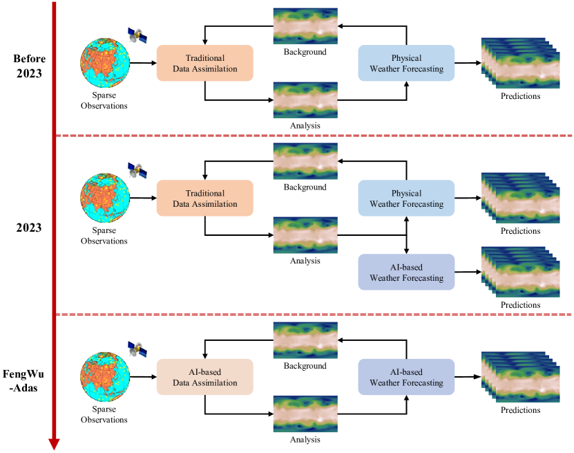
The weather forecasting system is important for science and society, and significant achievements have been made in applying artificial intelligence (AI) to medium-range weather forecasting. However, existing AI-based weather forecasting models still rely on analysis or reanalysis products from the traditional numerical weather prediction (NWP) systems as initial conditions for making predictions, preventing them from being fully independent systems. As a crucial component of an end-to-end global weather forecasting system, data assimilation is vital in generating initial states for forecasting. In this paper, we present an AI-based data assimilation model, i.e., Adas, for global weather variables, which learns to generate the analysis from the background and sparse observations. Different from existing assimilation methods, Adas employs the gated convolution module to handle sparse observations and the gated cross-attention module for capturing the interactions between observations and background efficiently, which are guided by the confidence matrix to represent the availability and quality of observations. Then, we combine Adas with the advanced AI-based weather forecasting model (i.e., FengWu) and construct the first end-to-end AI-based global weather forecasting system: FengWu-Adas. Experiments demonstrate that Adas can assimilate the simulated global observations with the AI-generated background through a one-year simulation and generate high-quality analysis stably in a cyclic manner. Based on the generated analysis, FengWu-Adas exhibits skillful performance and outperforms the Integrated Forecasting System (IFS) in weather forecasting over seven days.
Keywords Data Assimilation Artificial Intelligence Medium-range Weather Forecast Deep Learning
1 Introduction
Driven by the advancements and maturity of AI, particularly deep learning techniques, scientific intelligence has been rapidly evolving with the aim of leveraging AI to promote scientific research and discovery. Within the field of atmospheric science, AI has achieved remarkable achievements in various areas, such as post-processing and bias correction (Yang et al., 2023; Mouatadid et al., 2023; Agrawal et al., 2023; Singh et al., 2022), downscaling (Harder et al., 2022; Chen et al., 2022), precipitation nowcasting (Ravuri et al., 2021; Gao et al., 2022; Zhang et al., 2023), climate forecasting (Ling et al., 2022), and medium-range weather forecasting (Pathak et al., 2022; Bi et al., 2023; Lam et al., 2022; Chen et al., 2023a, b). Some AI-based models have demonstrated highly competitive forecasts compared to the deterministic forecasts of the state-of-the-art NWP system, i.e., the IFS from the European Centre for Medium-Range Weather Forecasts (ECMWF). These models are usually trained on reanalysis dataset (e.g., ERA5 (Hersbach et al., 2020) from ECMWF) and allow much lower computational costs and easier deployment for operational forecasting. Despite drawbacks such as forecast smoothness and bias drift (Ben-Bouallegue et al., 2023), AI approaches have shown the immense potential of data-driven modeling in weather prediction, offering a new paradigm for meteorological forecasting.
Despite the fact that significant progress has been made, the AI-based weather forecasting models mentioned earlier still require analysis products generated through the process of data assimilation in the traditional NWP system for making predictions. Specifically, data assimilation aims to obtain the best estimate of the true state of the Earth system (known as the analysis) and provide an accurate initial state for weather prediction, thereby improving the forecast performance. In a self-sustaining global weather forecasting system, data assimilation is a critical component to ensure the long-term stability of the system. Observations serve as crucial sources of information for data assimilation since they are the closest representation of the true state of the atmosphere. For example, the earliest initial conditions were obtained by interpolating observations onto the grid points of the state space (Richardson, 1922). Modern data assimilation techniques are usually achieved by integrating observations with the short-range forecasts (i.e., the background), primarily including two categories: Kalman filters and variational methods (Asch et al., 2016; Rabier and Liu, 2003). The main motivation for introducing the background, or the first guess, lies in the incomplete nature of observations. The sparsity of observations leads to a much lower dimensionality compared to the state vector, resulting in low-quality interpolation analysis. Besides, not all state variables can be observed directly.
Currently, AI methods have primarily been integrated into specific processes within data assimilation to address the limitations of traditional data assimilation techniques (Buizza et al., 2022; Cheng et al., 2023b). For instance, implicit neural representations (INRs) (Li et al., 2023) and various autoencoders (AEs) (Peyron et al., 2021; Melinc and Zaplotnik, 2023; Amendola et al., 2021) have been employed as reduced-order-models (ROMs) to tackle high-dimensional challenges. These methods replace classical linear models such as Proper Orthogonal Decomposition (POD) (Cheng et al., 2023a; Pawar and San, 2022) in latent assimilation, providing an efficient framework for the representation and reconstruction of state variables in the latent space. Neural networks have also been utilized to derive tangent-linear and adjoint models in 4D variational (4D-Var) data assimilation (Hatfield et al., 2021), provide localization functions for ensemble Kalman filters (EnKF) (Wang et al., 2023) and estimate error covariance matrix (Cheng and Qiu, 2022; Penny et al., 2022). Moreover, there exist strong mathematical similarities between machine learning and data assimilation, particularly the variational data assimilation (Geer, 2021), which enables the optimization of the cost function in variational data assimilation using auto-differentiation (Melinc and Zaplotnik, 2023). However, these studies have not involved altering the algorithms of data assimilation.
While traditional data assimilation techniques are underpinned by rigorous mathematical theory and physical priors, they inevitably rely on certain assumptions as prerequisites. In practical operational applications, they often face constraints due to high computational costs, necessitating various approximations for solution (Carrassi et al., 2018). In situations where supervised information is available, neural networks are expected to automatically capture the correlations among data during the assimilation (Fablet et al., 2021). While some efforts (de Almeida et al., 2022; Wu et al., 2021) have been made, they simply feed the data into networks without any specialized design, such as addressing the sparsity of observations. Instead of mapping the state space to the observation space through the observation operator to reduce dimension, the lower computational costs of neural networks allow data assimilation to be performed on the grid points of the state space, making it a promising direction for developing AI-based data assimilation methods (Kadow et al., 2020).
In this study, we present Adas, a novel neural network model designed for the data assimilation of global weather variables. Inspired by the gating mask in gated convolution (Yu et al., 2019) and the error covariance matrix in traditional data assimilation techniques, we introduce the confidence matrix to evaluate the availability and quality of observations during the data assimilation. Adas employs the gated convolution module to handle sparse observations and the gated cross-attention module for capturing the interactions between the background and observations efficiently. The prediction of the advanced AI-based weather forecasting model, FengWu (Chen et al., 2023a), is used to generate the background for data assimilation. In return, the analysis of Adas is then used as the initial state of FengWu for making predictions at the next time step, thus forming the first end-to-end AI-based global weather forecasting system: FengWu-Adas. Experiments demonstrate that Adas can capture the distribution patterns of the background error and assimilate the simulated global observations with the background effectively. Based on the generated high-quality analysis, FengWu-Adas runs stably in a cyclic and self-contained manner through a one-year simulation. The system outperforms the IFS in weather forecasting over seven days. In addition, ablation studies with fixed observation locations and random initialization have demonstrated skillful assimilation ability and robustness of the system.
2 Methods
In this section, we describe the framework and techniques of our method. Section 2.1 formulates the problem and shows the framework of our end-to-end global weather forecasting system. Section 2.2 elaborates on the designs of our network and details of customized modules for data assimilation. Finally, section 2.3 gives the loss function to supervise the neural network training.
2.1 Problem Formulation
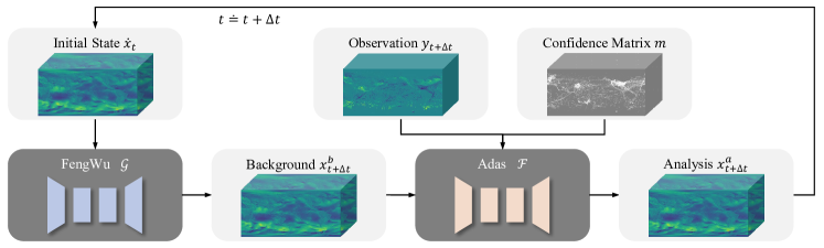
Our objective is to construct an AI-based end-to-end global weather forecasting system, FengWu-Adas, whose framework is shown in Figure 2. The short-range forecast (i.e., 6 hours) of FengWu is used as the background for data assimilation, and Adas produces the analysis from the background and sparse observations. Then, the generated analysis is used as the initial state of FengWu at the next time step in a cyclic manner. Once the observations are available, the system can operate stably for long term and generate high-quality analysis. For the given initial state denoted as at time , FengWu can make multi-step predictions , , …, at time , , …, in an auto-regressive manner, where denotes the time index and is the temporal spacing of single-step prediction. Considering that the accuracy of the background will directly affect the quality of the analysis, the single-step prediction of FengWu, which is denoted as , is used as the background , i.e.,
| (1) |
After obtaining the observations at the corresponding time, confidence levels ranging from 0 to 1 can be assigned to each datum based on the availability and quality of the observation source, thereby generating the confidence matrix. The confidence matrix , serving as supplementary information, is then sent into Adas along with observations for assimilation. Denote Adas as , then the process of data assimilation to generate the analysis at time can be expressed as
| (2) |
Subsequently, the analysis of Adas will be the next initial state, or the input of FengWu at next time, i.e.,
| (3) |
and so on, in a cyclic manner. By minimizing the loss function between the analysis and ground truth , we optimize the trainable parameters of Adas in a supervised fashion. During training, the parameters of FengWu are frozen and do not participate in iterations and updates. The initialization of the system, i.e., the initial state for forecasting at the first time step, can be arbitrary. In section 3.2, we will demonstrate that even with a completely random initial state to start, our system can rapidly stabilize and maintain long-term operation without performance degradation.
2.2 Network Architecture
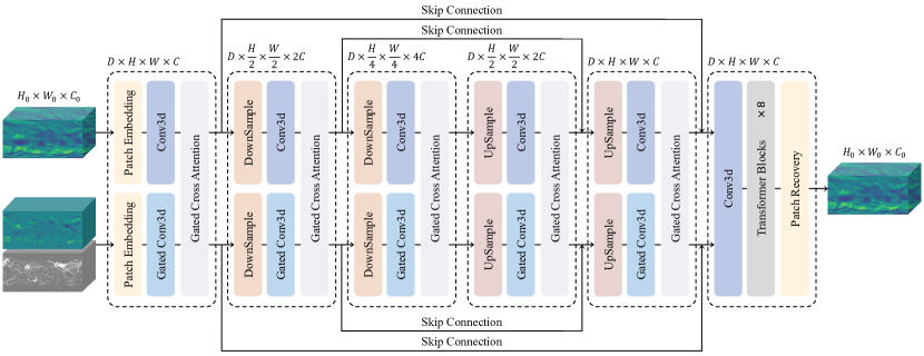
Adas takes the background, observations, and the confidence matrix as inputs and outputs the corresponding analysis as illustrated in Figure 3. All the inputs with a shape of are converted into a unified latent shape of through the patch embedding module so that the network can capture their spatial relationships in the 3D mesh. and represent the number of grid points in the latitude and longitude directions, respectively, and the channel represents the number of variables. The 3D atmospheric variables and 2D surface variables are embedded into the latent space independently and then concatenated together, where the information at each grid point is represented by a -dimensional vector. and correspond to the number of grid points in the latitude and longitude directions after embedding, and represents the number of levels in the vertical direction. Subsequently, the hierarchical UNet (Ronneberger et al., 2015) extracts features from inputs with normal convolution and gated convolution, along with efficient information interactions through the gated cross-attention module. Both the gated convolution and the gated cross-attention are guided by the confidence matrix, which is updated together with the features to represent the availability and quality of observations. The UNet structure can extract multi-scale features through down- and up-sampling and skip connections. After feature fusion through a convolutional layer, the features are sent into a series of Transformer (Vaswani et al., 2017; Dosovitskiy et al., 2020) blocks and then recovered to the original size. The convolutional operation can bring inductive bias of locality, and the attention mechanism enables the model to capture long-range dependencies. Below, we describe the technical details of the gated convolution module and the gated cross-attention module.
Gated Convolution.
Gated convolution (Yu et al., 2019) is a convoluional operation based on soft-gating, which employs continuous masks ranging between 0 and 1 to represent the degree of validity for each pixel. Originally, the gating mask in gated convolution was learned automatically from data at each layer, and the output features were weighted by it. In Adas, the confidence matrix of our method can serve as the gating mask. By using the confidence matrix as input for each layer and updating it explicitly, we propose an improved form of gated convolution to provide a more complete representation for sparse observations. The guidance of the confidence matrix can help the network extract features more effectively and capture the interactions between the background and observations more efficiently in the gated cross-attention module. Specifically, each value in the confidence matrix signifies the degree of confidence associated with corresponding observation values, and the confidence matrix is dynamically updated to guide the varying confidence levels of different layers. Let the subscript and represent the input and output of each layer, respectively, then the gated convolution and the update rule of the confidence matrix can be formulated as
| (4) |
| (5) |
where represents element-wise multiplication. The activation ensures that the values of the confidence matrix are between 0 and 1, and the activation funtion for features can be arbitrary. We use the activation here, which has been proven to be a better choice than (Hendrycks and Gimpel, 2016; Elfwing et al., 2018; Ramachandran et al., 2017). The gated convolution module can provide a more complete representation for observations and improve the quality of feature fusion.
Gated Cross-Attention.
The cross-attention mechanism is introduced to capture the interactions between the background and observations, but treating observations at different locations with different confidence levels equally is clearly unreasonable. Especially for observations with low confidence levels, directly calculating cross-attention may have negative guidance on the background. To address this issue, we propose the gated cross-attention module, which is also guided by the confidence matrix. Specifically, when the observations are used as the condition of cross-attention, the background is aligned with them at first, ensuring that observations influence the background in proportion to the confidence levels. After calculating the cross-attention, the remaining proportion of the background that does not participate in the operation will be added back. Conversely, the background fully influences observations since all values in the background have high confidence levels generally, which can correct the observations with low confidence levels. Therefore, the confidence matrix needs to be updated accordingly, which is also implemented through a convolutional layer with activation. The process of gated cross-attention can be expressed as
| (6) |
| (7) |
| (8) |
where the inputs of correspond to query (), key () and value (), respectively. The gated cross-attention module utilizes information for interactions selectively based on confidence levels, which can effectively avoid the negative impact of low-quality data.
2.3 Training Loss
The Mean Absolute Error (MAE) loss, also known as L1 loss, is employed to supervise the training of the neural network. In multivariate optimization, an issue of imbalanced optimization arises when there are significant differences in the magnitudes of losses for different variables. Therefore, it is necessary to weigh the losses for different variables. Instead of setting the weights manually, the losses for each variable (i.e., each channel) are automatically weighted to have the same magnitude in our training. The weights of each channel and the final loss can be expressed as
| (9) |
where and respectively represent the weight and loss of the -th channel, .
3 Results
We conduct long-term forecasting-assimilation experiments and multi-step weather forecasting experiments to evaluate the stability and performance of our system. In this section, we show the experimental setup and results to prove the effectiveness of the proposed method. Section 3.1 introduces the data used to carry out the experiments and provides the hyperparameters for model training and metrics for evaluation. Section 3.2 displays the metrics and visual analysis of the cyclic forecasting-assimilation experiments, and ablation studies are also shown to demonstrate the robustness and stability of our system. Section 3.3 gives the comparison of forecasting skills between the IFS and FengWu-Adas, further confirming the superior performance of our system.
3.1 Experimental Setup
To have sufficient data for model training, ERA5 is used as the ground truth and source of the simulated observations. ERA5 is a global atmospheric reanalysis archive containing hourly weather variables such as temperature, geopotential, wind speed, humidity, etc. A subset of ECMWF’s ERA5 dataset for 40 years, from 1979 to 2018, is chosen to train and evaluate the model. We choose to conduct experiments on a total of 68 variables at a resolution of 1.40525° ( grid points), including five atmospheric variables with 13 pressure levels (i.e., 50hPa, 100hPa, 150hPa, 200hPa, 250hPa, 300hPa, 400hPa, 500hPa, 600hPa, 700hPa, 850hPa, 925hPa, and 1000hPa), and four surface variables. Specifically, the atmospheric variables are geopotential (z), temperature (t), relative humidity (r), zonal component of wind (u) and meridional component of wind (v), whose 13 sub-variables at different vertical level are presented by abbreviating their short name and pressure levels (e.g., z500 denotes the geopotential at a pressure level of 500 hPa), and the surface variables are 10-meter zonal component of wind (u10), 10-meter meridional component of wind (v10), and 2-meter temperature (t2m). Following a common protocol demonstrated by FengWu (Chen et al., 2023a), the data from 1979-2015 are used for training, 2016-2017 for validation, and 2018 for testing.
The simulated observations are obtained by adding random Gaussian noise to the ground truth and then masking it, and the mask is used as the simulated confidence matrix for data assimilation. To improve the robustness of observation locations, the masks are generated randomly, with a mask ratio of 85%. The patch size of Adas in the experiments is set to 2, which means and , and the dimension is 96. The model is trained for 50 epochs using the AdamW optimizer (Loshchilov and Hutter, 2018) and OneCycleLR scheduler (Smith and Topin, 2019). The learning rate starts from 5e-6, warms to a maximum value of 5e-4 for ten epochs, and then decays gradually to 5e-8. After training, Adas can perform data assimilation directly on a single GPU in only about 0.055 seconds. Below, we introduce the metrics used for evaluation in the experiments.
RMSE represents the latitude-weighted root mean square error, which is a statistical metric widely used in geospatial analysis and climate science to assess the accuracy of a model’s forecasts or estimates of variables across different latitudes. Latitude weighting is a common strategy to account for the varying area represented by different latitudes on a spherical Earth. Given the estimate and its ground truth for the -th channel at time , the RMSE is defined as
| (10) |
where and denote the indices for each grid along the latitude and longitude indices, respectively, and is the latitude of point . For the forecast and its ground truth for the -th channel with lead time , the RMSE is defined as
| (11) |
where is the total number of test time slots.
Bias represents the latitude-weighted mean error (Ben-Bouallegue et al., 2023), a statistical metric to assess the bias of a model’s forecasts or estimates of variables across different latitudes. An ideal system should have a bias close to 0. Given the estimate and its ground truth for the -th channel at time , the Bias is defined as
| (12) |
In addition, ACC (the latitude-weighted anomaly correlation coefficient) is also a widely used statistical metric that reflects the model’s ability to capture anomalies (departures from the long-term averaged climatology). Owing to the phenomenon that lower RMSE is usually accompanied by higher ACC, it is omitted in this study.
3.2 Cyclic Forecasting-Assimilation Experiments
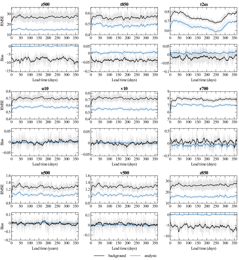
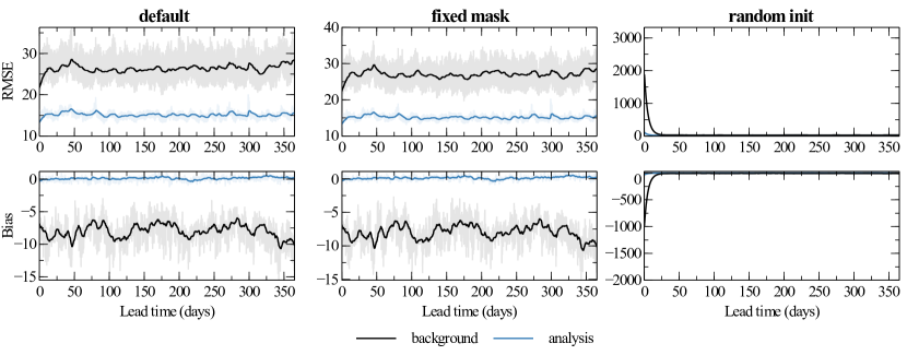
Firstly, a year-long cycle of the forecasting-assimilation experiment is conducted on the 2018 test set. The system is initialized using the ERA5 data at the first time step, which serves as the initial state for the first-step forecasting. The experiment proceeds with alternating weather forecasting and data assimilation steps: the single-step forecast provides the background for data assimilation, and the analysis is used as the initial state for the next forecasting step. Once the system is initialized, ERA5 data is invisible throughout the whole year, except for generating simulated observations. Figure 4 illustrates the variations in RMSE and Bias for the main variables of the system over the year. The background and the analysis are represented by black and blue colors, respectively. To enhance clarity, the original data is presented with reduced opacity, while the solid lines indicate the smoothed values after the exponential moving average (EMA) with a smoothing factor of 95%. Both the background error and the analysis error are always maintained at a low level, showing the long-term stability of the system and the ability to generate accurate analysis based on Adas. As expected, the analysis exhibits lower RMSE compared to the background. It is worth noting that the Bias of the analysis for all variables remains stable at around 0, revealing the system’s potential to eliminate bias drift of AI-based forecasting models and maintain conservation. Furthermore, the RMSE and Bias of the analysis demonstrate better stability than the background, characterized by smaller error fluctuations (as shown by the transparent original data).
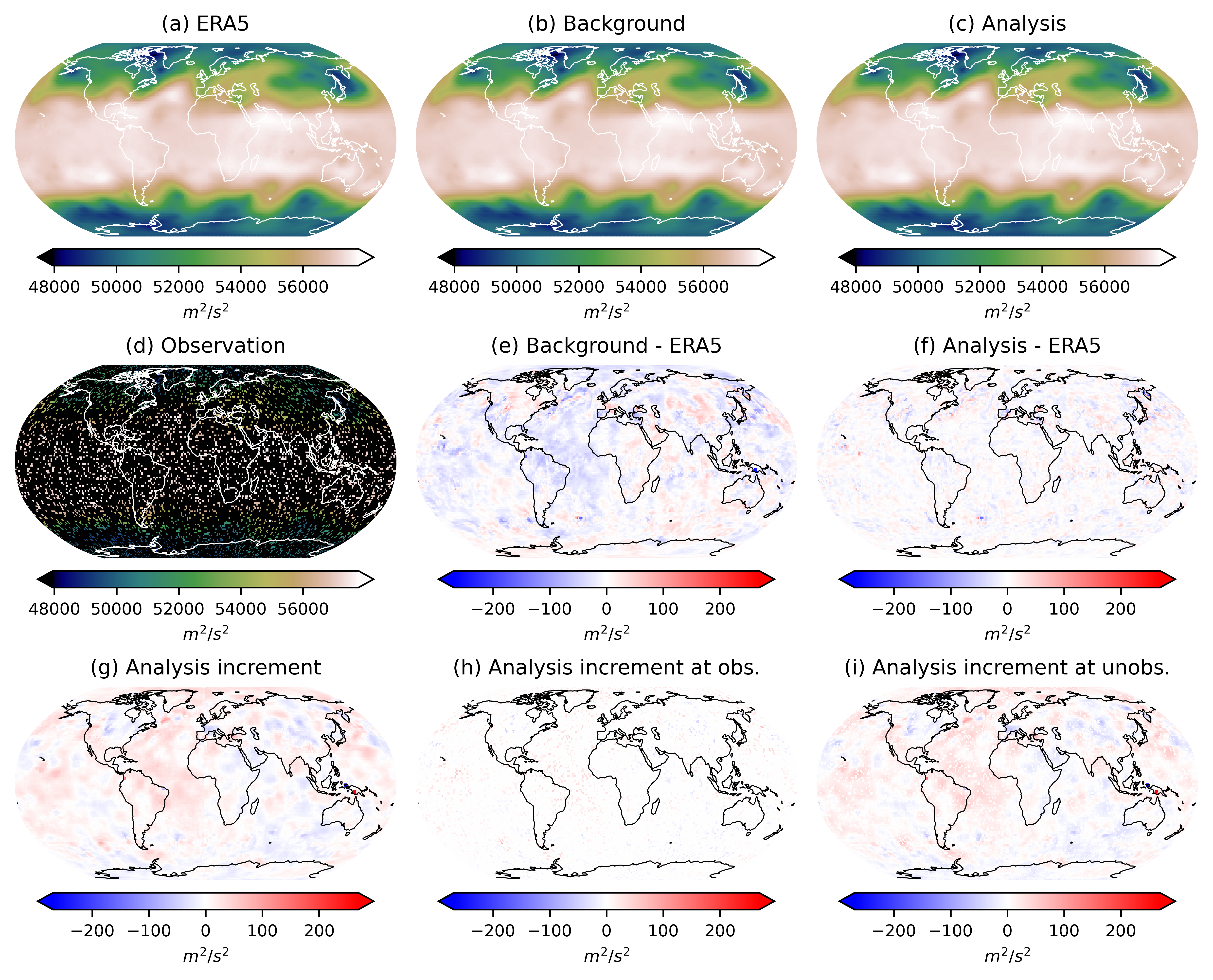
The visualizations for z500 in the data assimilation, along with the error distributions and analysis increments, are presented in Figure 5. z500 is a widely reported variable in previous data assimilation studies. The visualization date-time is randomly selected at 2018-01-26 06:00UTC, where the background is obtained from FengWu by performing single-step forecasting of the analysis at 2018-01-26 00:00UTC. Panels (a)-(c) display the visualizations of ERA5 (i.e., the ground truth), the background, and the analysis, respectively, and the visual differences between them are very small. Panel (d) shows the randomly generated simulated observations corresponding to the given time. Panels (e) and (f) depict the error distributions of the background and the analysis relative to ERA5, respectively, while panel (g) represents the analysis increments (i.e., the analysis minus the background). It can be observed that the errors of the analysis are significantly reduced after assimilation, and their distribution becomes more erratic and irregular. The analysis increments exhibit a distribution similar to the background errors but appear more continuous and smooth, indicating that Adas captures the error distribution of the background effectively. Panels (h) and (i) present the analysis increments at observed and unobserved locations, respectively, with no significant difference in magnitude between them. This indicates that skillful assimilation results can be achieved even at unobserved locations, further validating the effectiveness of our approach.
Most observation locations are generally fixed in real-world scenarios. Using a completely random mask for testing not only deviates from reality but also poses potential issues in the cyclic experiments. Specifically, a random mask implies that any position has the probability of being observed. When the number of steps in the cyclic experiments is sufficiently large, the observation positions would approximately cover the whole world, which is clearly unrealistic. To address this concern, an experiment with the fixed mask is conducted, and the corresponding RMSE and Bias for z500 are shown in the second column of Figure 6. Compared to the first column with default settings (i.e., random mask), there is almost no visible difference. This indicates that even when observations are absent from the majority of locations, our system performs equally well. The proposed method propagates sparse observation information to other regions effectively, providing high-confidence information for both observed and unobserved locations, which is consistent with the results presented in panels (h) and (i) of Figure 5. This not only proves the skillful assimilation ability of our system but also reflects the robustness to different observation situations to some extent.
Furthermore, a completely random initial state is used to initialize the system to evaluate the stability of FengWu-Adas based on the fixed mask experiment. The last column in Figure 6 shows the corresponding RMSE and Bias for z500. As can be observed, the first-step forecast after random initialization produces a terrible performance, with RMSE and Bias reaching 3332.19 and -1981.11, respectively. However, the corresponding values decrease to 160.579 and -39.7953 only after one step of data assimilation. After one day (i.e., four steps), the errors quickly converge to a stable state with the same levels of stable metrics as the default settings. Please note that the solid lines represent the smoothed values, and the transparent original data remains consistently low throughout the year due to fast convergence, making it almost imperceptible in the graph. This indicates that in situations where the confidence level of the background is very low or even completely untrustworthy, an acceptable analysis can be obtained after data assimilation. Even if the system encounters a malfunction that leads to complete derailment of the forecast, it can correct back to a stable state in a short period of time without affecting subsequent operations.
3.3 Multi-step Weather Forecasting Experiment
An important role of data assimilation is to provide initial states for forecasting. After the above cyclic forecasting-assimilation experiments, the analyses for 2018 can be generated. In order to further evaluate the quality of data assimilation and the performance of our system, the analyses are used as the initial states for multi-step weather forecasting. Figure 7 shows the comparison of RMSE skill over seven days for the main variables of our system and the IFS. The red and blue lines represent the IFS and our system, respectively. Throughout all 28 steps within seven days, our system consistently outperforms the IFS in terms of forecasting accuracy for all variables. The normalized RMSE difference between model A and baseline B is calculated by . For the 2-meter temperature (t2m), our normalized RMSE differences are nearly 30% lower than IFS at early lead times, while the majority of other variables are between 10-30%. Both systems use their own analyses as the initial states and compute RMSE against ERA5, which avoids the unfairness of comparison to some extent.
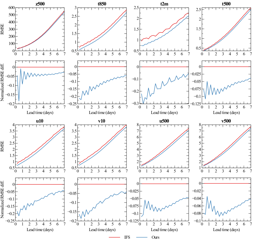
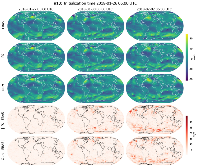
Figure 8 illustrates the visualizations for u10 and the absolute errors of our system and IFS at different lead times. The initialization date-time is set at 2018-01-26 06:00 UTC, which is the same as Figure 5, and the columns are three lead times, 1, 4, and 7 days, with the date-times indicated in the column headers. The top three rows depict the visualizations of ERA5 (i.e., ground truth), the forecasts of IFS, and the forecasts of our system, while the bottom two rows correspond to the absolute errors between ERA5 and the forecasts of both systems. In comparison with skill metrics, the visualizations provide a more intuitive representation of the forecasts and error distributions. Similar to most AI-based weather forecasting studies, our system exhibits error patterns that resemble those of IFS, but the absolute values of the forecasting errors are reduced to varying degrees across most locations.
4 Discussion
This paper presents Adas, a novel AI-based data assimilation model for global weather variables, which learns to generate the analysis from the background and sparse observations. Drawing inspiration from the gating mask in gated convolution and the error covariance matrix in traditional data assimilation techniques, the confidence matrix is introduced to represent the availability and quality of observations. Adas employs the gated convolution module to handle sparse observations and the gated cross-attention module to efficiently capture the interactions between observations and background, which are guided by the confidence matrix. By integrating Adas with the advanced AI-based weather forecasting model, FengWu, we establish the first end-to-end AI-based global weather forecasting system: FengWu-Adas. Simulated experiments demonstrate that Adas can capture the background error distribution patterns and generate high-quality analysis from the AI-generated background and global observations. Furthermore, FengWu-Adas exhibits skillful performance and stability and outperforms the IFS in weather forecasting over seven days.
Due to the unavailability of sufficient real observational data for model training, the experiments are conducted using simulated observations generated from ERA5, making it impossible to achieve a fully fair and realistic comparison with the IFS. This serves as the primary limitation of this study and a major direction for our future exploration. A potential solution could involve utilizing the paradigm based on pre-training with reanalysis and fine-tuning with real observational data (Scholz et al., 2023). Nevertheless, the method proposed in this study is universal and can be directly extended to the assimilation of real observational data theoretically. The reanalysis dataset remains important for scientific research and practical applications, thus developing physical models is still crucial. Therefore, our purpose is not to replace the traditional NWP systems but to demonstrate AI methods’ potential in tackling real-world challenges. Both physical techniques and AI methods have their own strengths and limitations, and they should be treated equally and considered as powerful tools for benefiting science and society. We believe that this is a meaningful exploration and look forward to the deployment and implementation of AI methods in operational systems in the future.
Acknowledgements
We acknowledge the ECMWF for their great efforts in storing and providing the invaluable datasets, which is very important for this work and the research community. We acknowledge the research team and service team in the Shanghai AI Laboratory for the provision of computational resources and infrastructure. We would also like to express our appreciation to Mr. Huihang Sun and Prof. Jiayuan Fan for their suggestion and valuable discussions during the conduction of this research.
References
- Agrawal et al. [2023] Shreya Agrawal, Rob Carver, Cenk Gazen, Eric Maddy, Vladimir Krasnopolsky, Carla Bromberg, Zack Ontiveros, Tyler Russell, Jason Hickey, and Sid Boukabara. A machine learning outlook: Post-processing of global medium-range forecasts. arXiv preprint arXiv:2303.16301, 2023.
- Amendola et al. [2021] Maddalena Amendola, Rossella Arcucci, Laetitia Mottet, César Quilodrán Casas, Shiwei Fan, Christopher Pain, Paul Linden, and Yi-Ke Guo. Data assimilation in the latent space of a convolutional autoencoder. In International Conference on Computational Science, pages 373–386. Springer, 2021.
- Asch et al. [2016] Mark Asch, Marc Bocquet, and Maëlle Nodet. Data assimilation: methods, algorithms, and applications. SIAM, 2016.
- Ben-Bouallegue et al. [2023] Zied Ben-Bouallegue, Mariana CA Clare, Linus Magnusson, Estibaliz Gascon, Michael Maier-Gerber, Martin Janousek, Mark Rodwell, Florian Pinault, Jesper S Dramsch, Simon TK Lang, et al. The rise of data-driven weather forecasting. arXiv preprint arXiv:2307.10128, 2023.
- Bi et al. [2023] Kaifeng Bi, Lingxi Xie, Hengheng Zhang, Xin Chen, Xiaotao Gu, and Qi Tian. Accurate medium-range global weather forecasting with 3d neural networks. Nature, pages 1–6, 2023.
- Buizza et al. [2022] Caterina Buizza, César Quilodrán Casas, Philip Nadler, Julian Mack, Stefano Marrone, Zainab Titus, Clémence Le Cornec, Evelyn Heylen, Tolga Dur, Luis Baca Ruiz, et al. Data learning: Integrating data assimilation and machine learning. Journal of Computational Science, 58:101525, 2022.
- Carrassi et al. [2018] Alberto Carrassi, Marc Bocquet, Laurent Bertino, and Geir Evensen. Data assimilation in the geosciences: An overview of methods, issues, and perspectives. Wiley Interdisciplinary Reviews: Climate Change, 9(5):e535, 2018.
- Chen et al. [2023a] Kang Chen, Tao Han, Junchao Gong, Lei Bai, Fenghua Ling, Jing-Jia Luo, Xi Chen, Leiming Ma, Tianning Zhang, Rui Su, et al. Fengwu: Pushing the skillful global medium-range weather forecast beyond 10 days lead. arXiv preprint arXiv:2304.02948, 2023a.
- Chen et al. [2023b] Lei Chen, Xiaohui Zhong, Feng Zhang, Yuan Cheng, Yinghui Xu, Yuan Qi, and Hao Li. Fuxi: A cascade machine learning forecasting system for 15-day global weather forecast. arXiv preprint arXiv:2306.12873, 2023b.
- Chen et al. [2022] Xuanhong Chen, Kairui Feng, Naiyuan Liu, Bingbing Ni, Yifan Lu, Zhengyan Tong, and Ziang Liu. Rainnet: A large-scale imagery dataset and benchmark for spatial precipitation downscaling. Advances in Neural Information Processing Systems, 35:9797–9812, 2022.
- Cheng and Qiu [2022] Sibo Cheng and Mingming Qiu. Observation error covariance specification in dynamical systems for data assimilation using recurrent neural networks. Neural Computing and Applications, 34(16):13149–13167, 2022.
- Cheng et al. [2023a] Sibo Cheng, Jianhua Chen, Charitos Anastasiou, Panagiota Angeli, Omar K Matar, Yi-Ke Guo, Christopher C Pain, and Rossella Arcucci. Generalised latent assimilation in heterogeneous reduced spaces with machine learning surrogate models. Journal of Scientific Computing, 94(1):11, 2023a.
- Cheng et al. [2023b] Sibo Cheng, César Quilodrán-Casas, Said Ouala, Alban Farchi, Che Liu, Pierre Tandeo, Ronan Fablet, Didier Lucor, Bertrand Iooss, Julien Brajard, et al. Machine learning with data assimilation and uncertainty quantification for dynamical systems: a review. IEEE/CAA Journal of Automatica Sinica, 10(6):1361–1387, 2023b.
- de Almeida et al. [2022] Vinícius Albuquerque de Almeida, Haroldo Fraga de Campos Velho, Gutemberg Borges França, and Nelson Francisco Favilla Ebecken. Neural networks for data assimilation of surface and upper-air data in rio de janeiro. Geoscientific Model Development Discussions, pages 1–23, 2022.
- Dosovitskiy et al. [2020] Alexey Dosovitskiy, Lucas Beyer, Alexander Kolesnikov, Dirk Weissenborn, Xiaohua Zhai, Thomas Unterthiner, Mostafa Dehghani, Matthias Minderer, Georg Heigold, Sylvain Gelly, et al. An image is worth 16x16 words: Transformers for image recognition at scale. arXiv preprint arXiv:2010.11929, 2020.
- Elfwing et al. [2018] Stefan Elfwing, Eiji Uchibe, and Kenji Doya. Sigmoid-weighted linear units for neural network function approximation in reinforcement learning. Neural networks, 107:3–11, 2018.
- Fablet et al. [2021] Ronan Fablet, Bertrand Chapron, Lucas Drumetz, Etienne Mémin, Olivier Pannekoucke, and François Rousseau. Learning variational data assimilation models and solvers. Journal of Advances in Modeling Earth Systems, 13(10):e2021MS002572, 2021.
- Gao et al. [2022] Zhihan Gao, Xingjian Shi, Hao Wang, Yi Zhu, Yuyang Bernie Wang, Mu Li, and Dit-Yan Yeung. Earthformer: Exploring space-time transformers for earth system forecasting. Advances in Neural Information Processing Systems, 35:25390–25403, 2022.
- Geer [2021] Alan J Geer. Learning earth system models from observations: machine learning or data assimilation? Philosophical Transactions of the Royal Society A, 379(2194):20200089, 2021.
- Harder et al. [2022] Paula Harder, Qidong Yang, Venkatesh Ramesh, Prasanna Sattigeri, Alex Hernandez-Garcia, Campbell Watson, Daniela Szwarcman, and David Rolnick. Generating physically-consistent high-resolution climate data with hard-constrained neural networks. arXiv preprint arXiv:2208.05424, 2022.
- Hatfield et al. [2021] Sam Hatfield, Matthew Chantry, Peter Dueben, Philippe Lopez, Alan Geer, and Tim Palmer. Building tangent-linear and adjoint models for data assimilation with neural networks. Journal of Advances in Modeling Earth Systems, 13(9):e2021MS002521, 2021.
- Hendrycks and Gimpel [2016] Dan Hendrycks and Kevin Gimpel. Gaussian error linear units (gelus). arXiv preprint arXiv:1606.08415, 2016.
- Hersbach et al. [2020] Hans Hersbach, Bill Bell, Paul Berrisford, Shoji Hirahara, András Horányi, Joaquín Muñoz-Sabater, Julien Nicolas, Carole Peubey, Raluca Radu, Dinand Schepers, et al. The era5 global reanalysis. Quarterly Journal of the Royal Meteorological Society, 146(730):1999–2049, 2020.
- Kadow et al. [2020] Christopher Kadow, David Matthew Hall, and Uwe Ulbrich. Artificial intelligence reconstructs missing climate information. Nature Geoscience, 13(6):408–413, 2020.
- Lam et al. [2022] Remi Lam, Alvaro Sanchez-Gonzalez, Matthew Willson, Peter Wirnsberger, Meire Fortunato, Alexander Pritzel, Suman Ravuri, Timo Ewalds, Ferran Alet, Zach Eaton-Rosen, et al. Graphcast: Learning skillful medium-range global weather forecasting. arXiv preprint arXiv:2212.12794, 2022.
- Li et al. [2023] Zhuoyuan Li, Bin Dong, and Pingwen Zhang. Latent assimilation with implicit neural representations for unknown dynamics. arXiv preprint arXiv:2309.09574, 2023.
- Ling et al. [2022] Fenghua Ling, Jing-Jia Luo, Yue Li, Tao Tang, Lei Bai, Wanli Ouyang, and Toshio Yamagata. Multi-task machine learning improves multi-seasonal prediction of the indian ocean dipole. Nature Communications, 13(1):7681, 2022.
- Loshchilov and Hutter [2018] Ilya Loshchilov and Frank Hutter. Fixing weight decay regularization in adam. 2018.
- Melinc and Zaplotnik [2023] Boštjan Melinc and Žiga Zaplotnik. Neural-network data assimilation using variational autoencoder. arXiv preprint arXiv:2308.16073, 2023.
- Mouatadid et al. [2023] Soukayna Mouatadid, Paulo Orenstein, Genevieve Flaspohler, Judah Cohen, Miruna Oprescu, Ernest Fraenkel, and Lester Mackey. Adaptive bias correction for improved subseasonal forecasting. Nature Communications, 14(1):3482, 2023.
- Pathak et al. [2022] Jaideep Pathak, Shashank Subramanian, Peter Harrington, Sanjeev Raja, Ashesh Chattopadhyay, Morteza Mardani, Thorsten Kurth, David Hall, Zongyi Li, Kamyar Azizzadenesheli, et al. Fourcastnet: A global data-driven high-resolution weather model using adaptive fourier neural operators. arXiv preprint arXiv:2202.11214, 2022.
- Pawar and San [2022] Suraj Pawar and Omer San. Equation-free surrogate modeling of geophysical flows at the intersection of machine learning and data assimilation. Journal of Advances in Modeling Earth Systems, 14(11):e2022MS003170, 2022.
- Penny et al. [2022] Stephen G Penny, Timothy A Smith, T-C Chen, Jason A Platt, H-Y Lin, Michael Goodliff, and Henry DI Abarbanel. Integrating recurrent neural networks with data assimilation for scalable data-driven state estimation. Journal of Advances in Modeling Earth Systems, 14(3):e2021MS002843, 2022.
- Peyron et al. [2021] Mathis Peyron, Anthony Fillion, Selime Gürol, Victor Marchais, Serge Gratton, Pierre Boudier, and Gael Goret. Latent space data assimilation by using deep learning. Quarterly Journal of the Royal Meteorological Society, 147(740):3759–3777, 2021.
- Rabier and Liu [2003] Florence Rabier and Zhiquan Liu. Variational data assimilation: theory and overview. In Proc. ECMWF Seminar on Recent Developments in Data Assimilation for Atmosphere and Ocean, Reading, UK, September 8–12, pages 29–43, 2003.
- Ramachandran et al. [2017] Prajit Ramachandran, Barret Zoph, and Quoc V Le. Searching for activation functions. arXiv preprint arXiv:1710.05941, 2017.
- Ravuri et al. [2021] Suman Ravuri, Karel Lenc, Matthew Willson, Dmitry Kangin, Remi Lam, Piotr Mirowski, Megan Fitzsimons, Maria Athanassiadou, Sheleem Kashem, Sam Madge, et al. Skilful precipitation nowcasting using deep generative models of radar. Nature, 597(7878):672–677, 2021.
- Richardson [1922] Lewis F Richardson. Weather prediction by numerical process. University Press, 1922.
- Ronneberger et al. [2015] Olaf Ronneberger, Philipp Fischer, and Thomas Brox. U-net: Convolutional networks for biomedical image segmentation. In Medical Image Computing and Computer-Assisted Intervention–MICCAI 2015: 18th International Conference, Munich, Germany, October 5-9, 2015, Proceedings, Part III 18, pages 234–241. Springer, 2015.
- Scholz et al. [2023] Jonas Scholz, Tom R Andersson, Anna Vaughan, James Requeima, and Richard E Turner. Sim2real for environmental neural processes. arXiv preprint arXiv:2310.19932, 2023.
- Singh et al. [2022] Manmeet Singh, Nachiketa Acharya, Aditya Grover, Suryachandra A Rao, Bipin Kumar, Zong-Liang Yang, Dev Niyogi, et al. Short-range forecasts of global precipitation using deep learning-augmented numerical weather prediction. arXiv e-prints, pages arXiv–2206, 2022.
- Smith and Topin [2019] Leslie N Smith and Nicholay Topin. Super-convergence: Very fast training of neural networks using large learning rates. In Artificial intelligence and machine learning for multi-domain operations applications, volume 11006, pages 369–386. SPIE, 2019.
- Vaswani et al. [2017] Ashish Vaswani, Noam Shazeer, Niki Parmar, Jakob Uszkoreit, Llion Jones, Aidan N Gomez, Łukasz Kaiser, and Illia Polosukhin. Attention is all you need. Advances in neural information processing systems, 30, 2017.
- Wang et al. [2023] Zhongrui Wang, Lili Lei, Jeffrey L Anderson, Zhe-Min Tan, and Yi Zhang. Convolutional neural network-based adaptive localization for an ensemble kalman filter. Journal of Advances in Modeling Earth Systems, 15(10):e2023MS003642, 2023.
- Wu et al. [2021] Pin Wu, Xuting Chang, Wenyan Yuan, Junwu Sun, Wenjie Zhang, Rossella Arcucci, and Yike Guo. Fast data assimilation (fda): Data assimilation by machine learning for faster optimize model state. Journal of Computational Science, 51:101323, 2021.
- Yang et al. [2023] Song Yang, Fenghua Ling, Lei Bai, and Jing-Jia Luo. Improving seasonal forecast of summer precipitation in southeastern china using cyclegan deep learning bias correction. Submitted to: Geophysical Research Letters. doi, 10, 2023.
- Yu et al. [2019] Jiahui Yu, Zhe Lin, Jimei Yang, Xiaohui Shen, Xin Lu, and Thomas S Huang. Free-form image inpainting with gated convolution. In Proceedings of the IEEE/CVF international conference on computer vision, pages 4471–4480, 2019.
- Zhang et al. [2023] Yuchen Zhang, Mingsheng Long, Kaiyuan Chen, Lanxiang Xing, Ronghua Jin, Michael I Jordan, and Jianmin Wang. Skilful nowcasting of extreme precipitation with nowcastnet. Nature, pages 1–7, 2023.