Topological complexity of spiked random polynomials and finite-rank spherical integrals

Abstract.

We study the annealed complexity of a random Gaussian homogeneous polynomial on the $N$-dimensional unit sphere in the presence of deterministic polynomials that depend on fixed unit vectors and external parameters. In particular, we establish variational formulas for the exponential asymptotics of the average number of total critical points and of local maxima. This is obtained through the Kac-Rice formula and the determinant asymptotics of a finite-rank perturbation of a Gaussian Wigner matrix. More precisely, the determinant analysis is based on recent advances on finite-rank spherical integrals by Guionnet-Husson [24] to study the large deviations of multi-rank spiked Gaussian Wigner matrices. The analysis of the variational problem identifies a topological phase transition. There is an exact threshold for the external parameters such that, once exceeded, the complexity function vanishes into new regions in which the critical points are close to the given vectors. Interestingly, these regions also include those where critical points are close to multiple vectors.

1. Introduction

In this paper, we study the complexity of finite-rank spiked random polynomials on the $N$-dimensional unit sphere $\mathbb{S}^{N-1}$. Specifically, we consider a random smooth function $f_{N}\colon\mathbb{S}^{N-1}\to\mathbb{R}$ of the form $f_{N}(\bm{\sigma})=m(\bm{\sigma})+H_{N}(\bm{\sigma})$, where the mean function $m$ is a sum of deterministic polynomials of finite degree and $H_{N}$ is an isotropic Gaussian random field on $\mathbb{S}^{N-1}$. Our goal is to analyze the exponential asymptotic behavior of the average number of total critical points and of local maxima of the random function $f_{N}$.

1.1. Model and results

We assume that the Hamiltonian $H_{N}$ is an homogeneous polynomial of degree $p\geq 3$, which we parametrize here as

$$H_{N}(\bm{\sigma})=\sum_{1\leq i_{1},\ldots,i_{p}\leq N}W_{i_{1},\ldots,i_{p}}\sigma_{i_{1}}\cdots\sigma_{i_{p}},$$ (1.1)

where $\bm{\sigma}=(\sigma_{1},\ldots,\sigma_{N})\in\mathbb{S}^{N-1}$ and $\bm{W}=(W_{i_{1},\ldots,i_{p}})_{1\leq i_{1},\ldots,i_{p}\leq N}\in(\mathbb{R}^{N})^{\otimes p}$ is a Gaussian symmetric tensor with independent entries up to symmetry. In particular, the couplings $W_{i_{1},\ldots,i_{p}}$ are given by

$$W_{i_{1},\ldots,i_{p}}\stackrel{{\scriptstyle d}}{{=}}\frac{1}{\sqrt{2N}}\frac{1}{p!}\sum_{\pi\in\mathfrak{S}_{p}}G^{\pi}_{i_{1},\ldots,i_{p}},$$

where $\bm{G}\in(\mathbb{R}^{N})^{\otimes p}$ is an order-$p$ tensor with i.i.d. standard Gaussian random variables $G_{i_{1},\ldots,i_{p}}$ and for a permutation $\pi\in\mathfrak{S}_{p}$ over $p$ elements, we let $G^{\pi}_{i_{1},\ldots,i_{p}}$ denote $G^{\pi}_{i_{1},\ldots,i_{p}}=G_{\pi(i_{1}),\ldots,\pi(i_{p})}$. Hence, $H_{N}$ is a centered Gaussian process on $\mathbb{S}^{N-1}$ whose covariance function is given by

$$\mathbf{E}\left[H_{N}(\bm{\sigma})H_{N}(\bm{\sigma^{\prime}})\right]=\frac{\langle\bm{\sigma},\bm{\sigma^{\prime}}\rangle^{p}}{2N}.$$

The Hamiltonian $H_{N}$ is referred to in physics as the spherical pure $p$-spin model. Given $r$ deterministic vectors $\bm{u}_{1}^{\ast},\ldots,\bm{u}_{r}^{\ast}\in\mathbb{S}^{N-1}$, where $r\geq 1$ is a finite integer number, we then define the random function $f_{N}\colon\mathbb{S}^{N-1}\to\mathbb{R}$ by

$$f_{N}(\bm{\sigma})=\sum_{i=1}^{r}\lambda_{i}\langle\bm{u}_{i}^{\ast},\bm{\sigma}\rangle^{k_{i}}+\sum_{1\leq i_{1},\ldots,i_{p}\leq N}W_{i_{1},\ldots,i_{p}}\sigma_{i_{1}}\cdots\sigma_{i_{p}}.$$ (1.2)

Here, $k_{1},\ldots,k_{r}\geq 3$ and $\lambda_{1}\geq\cdots\geq\lambda_{r}\geq 0$.

Our goal is to characterize the annealed complexity of the high-dimensional random function $f_{N}$. More precisely, if for any open set $B\subset\mathbb{R}$ we let $\text{Crt}_{N}^{\text{tot}}(B)$ denote the number of total critical points of $f_{N}$ at which $f_{N}\in B$ and $\text{Crt}_{N}^{\text{max}}(B)$ the number of such local maxima, we wish to understand the large-$N$ asymptotics of the expected number of total critical points and of local maxima of $f_{N}$, i.e.,

$$\lim_{N\to\infty}\frac{1}{N}\log\mathbf{E}\left[\text{Crt}_{N}^{\text{tot}}(B)\right]\quad\text{and}\quad\lim_{N\to\infty}\frac{1}{N}\log\mathbf{E}\left[\text{Crt}_{N}^{\text{max}}(B)\right].$$

Early research into the complexity of random polynomials of the form (1.2) was conducted in physics by Crisanti-Sommers [18] for $\lambda_{1}=\ldots=\lambda_{r}=0$, that is, in the case of spherical pure spin glasses. A mathematically rigorous computation of the annealed complexity of the same pure noise model was provided by Auffinger-Ben Arous-C̆erný [6]. Further work [22] by Fyodorov analyzed the complexity of the spherical pure spin glass model in a random magnetic field whose Hamiltonian corresponds to (1.2) with $r=k=1$. When $r=1$ and $k=p$ the random function $f_{N}$ corresponds to the spiked tensor model, introduced in [34] in the context of high-dimensional statistical inference and whose complexity was studied by Ben Arous-Mei-Montanari-Nica [15]. More generally, when $r=1$, the model (1.2) is known as the “$(p,k)$ spiked tensor model” [5].

Our main result is the following. We show that there exists an upper semi-continuous function $\Sigma^{\text{tot}}$, called the total complexity function, such that

$$-\inf_{x\in B^{\circ}}-\Sigma^{\text{tot}}(x)\leq\liminf_{N\to\infty}\frac{1}{N}\log\mathbf{E}\left[\text{Crt}_{N}^{\text{tot}}(B)\right]\leq\limsup_{N\to\infty}\frac{1}{N}\log\mathbf{E}\left[\text{Crt}_{N}^{\text{tot}}(B)\right]\leq-\inf_{x\in\overline{B}}-\Sigma^{\text{tot}}(x).$$ (1.3)

That is, we establish a weak large deviation principle (LDP) in the speed $N$ and with good rate function $-\Sigma^{\text{tot}}$. We obtain a similar result for local maxima. The strategy of proof relies first on the Kac-Rice formula that reduces the complexity of the landscape to the study of the determinant of a multi-rank spiked Gaussian Wigner matrix and then on the determinant asymptotics of such large random matrix. The determinant analysis in the case of a finite-rank perturbation requires technical challenges. To this end, recent advances on finite-dimensional spherical integrals obtained by Guionnet-Husson [24] are needed to tackle the large deviations of Gaussian Wigner matrices in the presence of a finite-rank perturbation. As a consequence of this variational problem, we identify the regions where the complexity function $\Sigma^{\text{tot}}$ vanishes and where the number of critical point is therefore sub-exponential. Moreover, we show that, as the parameters cross an exact threshold, there are new regions of zero complexity in which the critical points are very close to the given vectors $\bm{u}_{1}^{\ast},\ldots,\bm{u}_{r}^{\ast}$. Interestingly, these regions include both those where the critical points are close to a single spike and those where the critical points are close to more than one spike. We refer the reader to the next subsections for more details on the strategy of proof and the related literature.

1.2. Motivation

The topological complexity of isotropic Gaussian random polynomials was initiated by Auffinger-Ben Arous-C̆erný [6] and by Auffinger-Ben Arous [4] on spherical spin glass models. This was followed by further work on the complexity of spiked random polynomials, in which a deterministic term that depends on a fixed vector is added to the Hamiltonian of spherical spin glasses. When the added term is linear, the deterministic part represents the external magnetic field aligned with the given direction and the complexity of this model was studied in [22, 9]. When the deterministic term is a polynomial of degree $p$, then it is the spiked tensor model that emerges from a statistical estimation problem [34] and whose complexity was analyzed in [15, 35]. In this paper, we focus on the spherical pure $p$-spin model in the presence of a deterministic term which favors all vectors that are close to $\bm{u}_{1}^{\ast},\ldots,\bm{u}_{r}^{\ast}\in\mathbb{S}^{N-1}$. The choice of our model is therefore natural within this framework. Although the function $f_{N}$ generalizes the spiked tensor model [15] for $r=1$ and $k=p$, our model is not directly related to an inference problem. However, we believe that studying the complexity of $f_{N}$ is relevant to understanding estimation problems that arise naturally in high-dimensional statistics, such as the multi-rank spiked tensor model that we present below. We consider the following inference task: we wish to recover the unknown signal vectors $\bm{u}_{1}^{\ast},\ldots,\bm{u}_{r}^{\ast}\in\mathbb{S}^{N-1}$ from a noisy observation of a tensor $\bm{Y}\in(\mathbb{R}^{N})^{\otimes p}$ of the form

$$\bm{Y}=\sum_{i=1}^{r}\lambda_{i}(\bm{u}_{i}^{\ast})^{\otimes p}+\bm{W}.$$ (1.4)

Here, $\bm{W}\in(\mathbb{R}^{N})^{\otimes p}$ is an order-$p$ Gaussian symmetric tensor and the parameters $\lambda_{1},\ldots,\lambda_{r}\geq 0$ are the signal-to-noise ratios. A natural estimator for the spikes $\bm{u}_{1}^{\ast},\ldots,\bm{u}_{r}^{\ast}$ is given by the maximum likelihood estimator (MLE). In the special case $r=1$, the MLE corresponds to the argmax of the random function $f_{N}$ with $k=p$ [34, 15]. Otherwise, the MLE is given by the argmax of the random function $F_{N}\colon\left(\mathbb{S}^{N-1}\right)^{r}\to\mathbb{R}$ defined by

$$F_{N}(\bm{\sigma}_{1},\ldots,\bm{\sigma}_{r})=\sum_{i=1}^{r}\lambda_{i}f_{N}(\bm{\sigma}_{i})-\sum_{1\leq i<j\leq r}\lambda_{i}\lambda_{j}\langle\bm{\sigma}_{i},\bm{\sigma}_{j}\rangle^{p},$$

where $f_{N}$ corresponds to (1.2) with $k_{i}=p$ for all $1\leq i\leq r$. Understanding the complexity of such landscapes requires additional efforts, especially with regard to the number of local maxima. Indeed, via the Kac-Rice formula, the problem reduces to the study of the large-$N$ limit of the determinant of a full-rank deformation of a large block matrix with dependent Gaussian blocks. This determinant analysis involves challenging techniques, such as the asymptotics of spherical integrals, to derive large deviations principles for the largest eigenvalue of such large random matrix. The study of the complexity of the multi-rank spiked tensor model therefore requires further effort and will be the subject of future work.

1.3. Related work

As mentioned above, early work on the complexity of high-dimensional landscapes was carried out in statistics and physics in the context of mean-field glasses and spin glasses [16, 30, 18, 17]. In the mathematical literature, the breakthrough paper was proposed by Fyodorov [21] on the model known as the “zero-dimensional elastic manifold”. Since then, the landscape properties have been studied for many different models. Of interest here, for instance, are the works on spherical spin glasses [6, 4, 39, 40] and in the presence of a deterministic term, e.g. [22, 15, 35, 37, 38, 9, 5]. The classical approach for counting the total number of such points is the Kac-Rice formula, which relates the average number of critical points to conditional averages of random matrix determinants. In most of the models studied so far, the random matrices appearing in the Kac-Rice formula are related to the Gaussian Orthogonal Ensemble (GOE). Recently, [11, 12] studied landscapes models with few distributional symmetries whose conditioned Hessian is a large random matrix with a non-invariant distribution.

In addition to the topological complexity question, models that depend on external parameters also provide a characterization of the landscape by identifying a topology trivialization transition when tuning the parameters. Specifically, there is an exact threshold between regimes where the complexity is positive and regimes where the complexity vanishes. Understanding these phase transitions can be useful in predicting the dynamics of optimization on the landscape. When complexity is non-positive and the number of critical points is thus sub-exponential, optimization should be easier, while conversely, when complexity is positive, optimization should be more difficult, since the number of critical points is exponentially large and algorithms can get trapped in a large number of critical points.

Optimization in high-dimensional landscapes is actually computationally hard. For the special case $p=2$, the model (1.2) reduces to the spiked matrix model introduced in [28]. This model exhibits a phase transition, known as the BBP transition [8], where there exists an order $1$ critical threshold $\lambda_{c}$ such that below $\lambda_{c}$, it is information-theoretical impossible to detect the signal vectors, and above $\lambda_{c}$, it is possible to detect the spikes by Principal Component analysis. The same phenomenon has been observed for the spiked tensor model. In particular, in the high-dimensional asymptotic regime, there is an order $1$ critical threshold $\lambda_{c}$ (depending on the order $p$), below which it is information-theoretical impossible to detect the spikes, and above, the MLE is known to be a good, consistent estimator. Computing the MLE is however NP-hard and finding a good algorithm to compute it quickly still remains a challenge (this phenomenon is known as a computational-to-statistical gap). For the rank-one case, it was shown heuristically in [34] that for the tensor power iteration method, it is possible to recover the spike provided $\lambda\gtrsim N^{\frac{p-2}{2}}$. This conjecture was rigorously proved in [26]. The same threshold was obtained for Langevin dynamics and gradient descent in [13]. Moreover, [14] investigated the tensor unfolding algorithm and proved that it is possible to recover successively the spike provided $\lambda\gtrsim N^{\frac{p-2}{4}}$, as conjectured in [34]. The sharp threshold $\lambda\gtrsim N^{\frac{p-2}{4}}$ was also achieved using Sum-of-Squares algorithms in [25].

We wish to emphasize that we address here the question of the average number of critical points, which in general may not be close to its typical value. A more representative quantity of the typical number of critical points is given by the quenched complexity, which corresponds to the large-$N$ asymptotics of the average of the logarithm of the number of critical points. In most of the models, the random variable $\text{Crt}^{\text{tot}}_{N}$ does not concentrate about its expectation, and quenched and annealed complexity differ from each other even at leading order, as in the case of the spiked tensor model [35]. The computation of the quenched complexity is a challenging problem and is usually based on a non-rigorous but exact approach involving the Kac-Rice formula and the replica theory from statistical physics (see e.g. [35, 32]). In the case of spherical pure spin glasses, it has been proved by means of a second moment analysis that the number of local minima and of critical points concentrates around its expectation [39, 40].

For a more complete review on the characterization of high-dimensional random landscapes we direct the reader to [36] and the references therein.

1.4. Outline of the proof

In the first part of the paper, we derive the variational formula (1.3) using the strategy developed by Auffinger-Ben Arous-C̆erný [6] and Auffinger-Ben Arous [4] for the Hamiltonian of spherical spin glasses and by Ben Arous-Mei-Montanari-Nica [15] for the spiked tensor model. In particular, the common approach for computing $\mathbf{E}\left[\text{Crt}^{\text{tot}}_{N}(B)\right]$ is the Kac-Rice formula which, in our case, reads

$$\mathbf{E}\left[\text{Crt}^{\text{tot}}_{N}(B)\right]=\int_{\mathbb{S}^{N-1}}\mathbf{E}\left[|\det(\text{Hess}\,f_{N}(\bm{\sigma}))|\cdot\mathbf{1}_{\{f_{N}(\bm{\sigma})\in B\}}\Big{|}\text{grad}\,f_{N}(\bm{\sigma})=0\right]\varphi_{\text{grad}\,f_{N}}(\bm{0})\text{d}\bm{\sigma}.$$

Here, $\text{grad}\,f_{N}$ and $\text{Hess}\,f_{N}$ denote the spherical gradient and Hessian of $f_{N}$ and $\varphi_{\text{grad}\,f_{N}}(\bm{0})$ is the density of $\text{grad}\,f_{N}$ at $\bm{0}$. Given the conditioned Hessian $H_{N}$ that appears in the Kac-Rice formula, the next step is to study the exponential asymptotics of the determinant of this random matrix, i.e., $\lim_{N\to\infty}\frac{1}{N}\log\mathbf{E}\left[\det(H_{N})\right]$. The difficulty in computing the annealed complexity therefore lies in the determinant asymptotics. In our case, the random matrix $H_{N}$ is a deformation of rank $r$ of a GOE matrix shifted by a term proportional to the identity, that is, $H_{N}$ is distributed as $\textnormal{GOE}(N)+\sum_{i=1}^{r}\gamma_{i}\bm{e}_{i}\bm{e}_{i}^{\top}-tI_{N}$. If $\rho_{\text{sc}}$ denotes the semicircle density on $[-2,2]$, for every compact $\mathcal{T}\subset\mathbb{R}$ we then show that

$$\lim_{N\to\infty}\sup_{t\in\,\mathcal{T}}\left|\frac{1}{N}\log\mathbf{E}\left[|\det(H_{N})|\right]-\int_{\mathbb{R}}\log|\lambda-t|\rho_{\text{sc}}(\lambda)\text{d}\lambda\right|=0,$$

which may be intuitive since the spectrum of a spiked Wigner matrix concentrates about the semicircle law. The proof relies on Theorem 1.2 of Ben Arous-Bourgade-McKenna [11]. We also wish to compute the annealed complexity of local maxima, for which the analogue is to study the large-$N$ limit of $\frac{1}{N}\log\mathbf{E}\left[\det(H_{N})\mathbf{1}_{\{H_{N}\preceq 0\}}\right]$. Here, the main challenge is to understand the asymptotic behavior of

$$\frac{1}{N}\log\mathbf{P}\left(\lambda_{\textnormal{max}}\left(\textnormal{GOE}(N)+\sum_{i=1}^{r}\gamma_{i}\bm{e}_{i}\bm{e}_{i}^{\top}\right)\leq t\right).$$

More precisely, we need the large deviations for the extreme eigenvalues of multi-rank spiked GOE matrices. The LDP for the largest eigenvalue when the deterministic perturbation is a rank-one matrix was provided by Maïda [31] and later applied in [15] to derive the complexity of local maxima for the spiked tensor model. When the perturbation is of finite rank, the difficulty lies in the asymptotics of finite-rank spherical integrals, also known as Harish-Chandra/Itzykson/Zuber integrals, defined by

$$\mathbf{E}_{e}\left[e^{\frac{N}{2}\sum_{i=1}^{k}\theta_{i}\langle e,X_{N}e\rangle}\right],$$

where $X_{N}$ is an $N\times N$ symmetric matrix, $\theta_{1}\geq\cdots\geq\theta_{k}\geq 0$, and the integration $\mathbf{E}_{e}$ is over vectors $e$ uniform on the unit sphere $\mathbb{S}^{N-1}$. Recently, Guionnet-Husson [24] showed that finite-rank spherical integrals are asymptotically equivalent to the product of rank-one spherical integrals. This then allowed to establish a LDP for the joint law of the $k$ largest eigenvalues of Gaussian Wigner matrices in the presence of multiple spikes (see Proposition 2.7 of [24]). We then combine this LDP result with classical techniques to obtain the LDP for the largest eigenvalue, thus generalizing the result of [31]. We specify that the result we present is actually more detailed and delicate to obtain since we express the random variables $\text{Crt}^{\text{tot}}_{N}$ and $\text{Crt}^{\text{max}}_{N}$ also as a function of the scalar product with $\bm{u}_{1}^{\ast},\ldots,\bm{u}_{r}^{\ast}$.

In the second part of the paper, we analyze the variational problem (1.3) and identify the regions where the complexity function vanishes and where the number of critical points is therefore sub-exponential. In particular, we identify a topological phase transition. We find an exact threshold for the parameters $\lambda_{1},\ldots,\lambda_{r}$ such that, crossing it, there are new regions of zero complexity where critical points are close to the given vectors. Interestingly, we find regions where critical points are close to more than one given vector. This generalizes the global picture observed in [15] in the presence of a single spike, by adding new regions of vanishing complexity where critical points are close to multiple spikes. Numerical evidence in the case $r=2$ suggests that local maxima with a large scalar product with the given vectors are located in those regions where critical points are close to a single spike.

1.5. Overview

An outline of the paper is given as follows. In Section 2 we state our main results on the landscape complexity of the random function $f_{N}$. In Section 3 we present our intermediate results, namely we compute the random matrix arising from the Kac-Rice formula and we derive the large deviation principle for the largest eigenvalue of a finite-rank spiked GOE matrix. The proofs of the main theorems are then provided in Section 4. Finally, in Section 5 we analyze the variational problem for the total complexity function and identify a topological phase transition.

Acknowledgements. I am grateful to my advisors Alice Guionnet and Gérard Ben Arous for proposing this subject, for invaluable discussions, and for many insightful inputs throughout this project. I also wish to thank Ben McKenna for early discussions on the project and Justin Ko and Slim Kammoun for their helpful comments. This work is supported by the ERC Advanced Grant LDRAM No. 884584. I also thank Gérard Ben Arous for welcoming me at the Courant Institute of Mathematical Sciences (NYU) during October 2022.

2. Main results

Our main results are exponential asymptotics of the average number of critical points and local maxima of the function $f_{N}$ introduced in (1.2). We first introduce the main object of our work. In the following, we let $\nabla_{\mathbb{S}^{N-1}}\,f_{N}(\bm{\sigma})$ and $\nabla^{2}_{\mathbb{S}^{N-1}}\,f_{N}(\bm{\sigma})$ denote the Riemannian gradient and Hessian at $\bm{\sigma}$ with respect to the standard metric on $\mathbb{S}^{N-1}$. Moreover, for a set $S\subset\mathbb{R}$, we let $\overline{S}$ and $S^{\circ}$ denote its closure and interior, respectively.

Definition 2.1.

Given Borel sets $M_{1},\ldots,M_{r}\subset[-1,1]$ and $B\subset\mathbb{R}$, we define the (random) total number $\textnormal{Crt}_{N}^{\textnormal{tot}}((M_{i})_{1\leq i\leq r},B)$ of critical points of the function $f_{N}$ that have overlap with $\bm{u}_{i}^{\ast}$ in $M_{i}$, for all $1\leq i\leq r$, and whose critical values are in $B$ by

$$\textnormal{Crt}_{N}^{\textnormal{tot}}((M_{i})_{1\leq i\leq r},B)\coloneqq\sum_{\begin{subarray}{c}\bm{\sigma}\in\mathbb{S}^{N-1}\colon\\ \nabla_{\mathbb{S}^{N-1}}\,f_{N}(\bm{\sigma})=0\end{subarray}}\mathbf{1}_{\{\langle\bm{\sigma},\bm{u}_{i}^{\ast}\rangle\in M_{i},\,1\leq i\leq r\}}\cdot\mathbf{1}_{\{f_{N}(\bm{\sigma})\in B\}},$$ (2.1)

and the corresponding number of critical points of index $\ell\in\{0,\ldots,N-1\}$ by

$$\textnormal{Crt}_{N}^{\ell}((M_{i})_{1\leq i\leq r},B)\coloneqq\sum_{\begin{subarray}{c}\bm{\sigma}\in\mathbb{S}^{N-1}\colon\\ \nabla_{\mathbb{S}^{N-1}}\,f_{N}(\bm{\sigma})=0\end{subarray}}\mathbf{1}_{\{\langle\bm{\sigma},\bm{u}_{i}^{\ast}\rangle\in M_{i},\,1\leq i\leq r\}}\cdot\mathbf{1}_{\{f_{N}(\bm{\sigma})\in B\}}\cdot\mathbf{1}_{\{i(\nabla^{2}_{\mathbb{S}^{N-1}}f_{N}(\bm{\sigma}))=\ell\}}.$$ (2.2)

Here, the index $i(\cdot)$ is the number of negative eigenvalues of $\nabla^{2}_{\mathbb{S}^{N-1}}\,f_{N}(\bm{\sigma})$. When $\ell=N-1$, the random variable $\textnormal{Crt}_{N}^{\textnormal{max}}((M_{i})_{1\leq i\leq r},B)$ denotes the number of local maxima that have overlap with $\bm{u}_{i}^{\ast}$ in $M_{i}$ and whose function values are in $B$. Similarly, when $\ell=0$, the random variable $\textnormal{Crt}_{N}^{\textnormal{min}}((M_{i})_{1\leq i\leq r},B)$ gives the number of local minima.

We next provide variational formulas for the large-$N$ asymptotics of the logarithm of the expectation $\mathbf{E}\left[\textnormal{Crt}_{N}^{\textnormal{tot}}((M_{i})_{1\leq i\leq r},B)\right]$ (resp. $\mathbf{E}\left[\textnormal{Crt}_{N}^{\textnormal{max}}((M_{i})_{1\leq i\leq r},B)\right]$) divided by $N$.

2.1. Annealed complexity of total critical points

Here we state our first annealed result on the total number of critical points. We first introduce the total complexity function.

Definition 2.2.

For Borel sets $M_{1},\ldots,M_{r}\subset[-1,1]$, we let $M=M_{1}\times\cdots\times M_{r}$ denote the Cartesian product and $D_{\Sigma}$ denote

$$D_{\Sigma}=\left\{\bm{m}=(m_{1},\ldots,m_{r})\in M\colon\sum_{i=1}^{r}m_{i}^{2}\in(0,1)\right\}\subseteq M.$$

For $(\bm{m},x)\in D_{\Sigma}\times\mathbb{R}$, we define

$$\begin{split}\Sigma(\bm{m},x)&=\frac{1}{2}(\log(p-1)+1)+\frac{1}{2}\log\left(1-\sum_{i=1}^{r}m_{i}^{2}\right)-\frac{1}{p}\sum_{i=1}^{r}\lambda_{i}^{2}k_{i}^{2}m_{i}^{2k_{i}-2}(1-m_{i}^{2})\\ &\quad+\frac{2}{p}\sum_{1\leq i<j\leq r}\lambda_{i}\lambda_{j}k_{i}k_{j}m_{i}^{k_{i}}m_{j}^{k_{j}}-\left(x-\frac{1}{p}\sum_{i=1}^{r}\lambda_{i}k_{i}m_{i}^{k_{i}}\right)^{2}+\Phi_{\ast}\left(\sqrt{\frac{2p}{p-1}}x\right),\end{split}$$

where $\Phi_{\ast}$ denotes the $\log$-potential of the semicircle distribution which is given by

$$\Phi_{\ast}(x)=\int_{\mathbb{R}}\log|\lambda-x|\rho_{\textnormal{sc}}(\textnormal{d}\lambda)=\begin{cases}\frac{x^{2}}{4}-\frac{1}{2}&\text{if}\>|x|\leq 2\\ \frac{x^{2}}{4}-\frac{1}{2}-\left(\frac{|x|}{4}\sqrt{x^{2}-4}-\log\left(\frac{|x|+\sqrt{x^{2}-4}}{2}\right)\right)&\text{if}\>|x|>2\end{cases}.$$ (2.3)

We then define the total complexity function $\Sigma^{\textnormal{tot}}\colon[-1,1]^{r}\times\mathbb{R}\to(\mathbb{R}\cup\{-\infty,+\infty\})$ by setting

$$\Sigma^{\textnormal{tot}}(\bm{m},x)=\begin{cases}\Sigma(\bm{m},y(\bm{m},x))&\text{if}\enspace\bm{m}\in D_{\Sigma}\\ -\infty&\text{if}\enspace\bm{m}\in D_{\Sigma}^{\text{c}}\end{cases},$$

where

$$y(\bm{m},x)=x-\sum_{i=1}^{r}\lambda_{i}(1-k_{i}/p)m_{i}^{k_{i}}.$$ (2.4)

The main result on the annealed complexity of total critical points is the following.

Theorem 2.3.

For any Borel sets $M_{1},\ldots,M_{r}\subset[-1,1]$ and $B\subset\mathbb{R}$, we have that

$$\limsup_{N\to\infty}\frac{1}{N}\log\mathbf{E}\left[\textnormal{Crt}_{N}^{\textnormal{tot}}((M_{i})_{1\leq i\leq r},B)\right] \leq\sup_{(\bm{m},x)\in\overline{M}\times\overline{B}}\Sigma^{\textnormal{tot}}(\bm{m},x),$$ (2.5)

$$\liminf_{N\to\infty}\frac{1}{N}\log\mathbf{E}\left[\textnormal{Crt}_{N}^{\textnormal{tot}}((M_{i})_{1\leq i\leq r},B)\right] \geq\sup_{(\bm{m},x)\in M^{\circ}\times B^{\circ}}\Sigma^{\textnormal{tot}}(\bm{m},x).$$ (2.6)

This gives a weak LDP in the speed $N$ and with good rate function $-\Sigma^{\textnormal{tot}}$.

As mentioned in the introduction, when $r=1$, the objective function $f_{N}$ reduces to

$$f_{N}(\bm{\sigma})=\lambda\langle\bm{u}^{\ast},\bm{\sigma}\rangle^{k}+\sum_{1\leq i_{1},\ldots,i_{p}\leq N}W_{i_{1},\ldots,i_{p}}\sigma_{i_{1}}\cdots\sigma_{i_{p}}.$$

This model is known as the $(p,k)$ spiked tensor model and was introduced in [5] to study the sharp asymptotics for the average number of local maxima. When $k=p$, the argmax of $f_{N}$ corresponds the MLE for the signal vector $\bm{u}^{\ast}$ and the complexity of this model was studied in [15]. In particular, Theorem 2.3 reduces to Theorem 1 of [15] in the special case $r=1$ and $k=p$.

2.2. Annealed complexity of local maxima

Next we present our second annealed result. We first introduce some important definitions, which will describe the asymptotic complexity of local maxima.

Definition 2.4.

For a sequence $\bm{\gamma}=(\gamma_{1},\ldots,\gamma_{r})\in\mathbb{R}^{r}$ arranged in descending order, $\gamma_{1}\geq\cdots\geq\gamma_{r}$, and $t\in\mathbb{R}$, we let $L(\bm{\gamma},t)$ denote the function given by

$$L(\bm{\gamma},t)=\sum_{\ell=1}^{r}I_{\ell}^{\bm{\gamma}}(t)\mathbf{1}_{\{\ell=\min\{i\colon\gamma_{i}\geq 1\}\}},$$ (2.7)

where $I_{\ell}^{\bm{\gamma}}\colon\mathbb{R}\to(\mathbb{R}\cup\{-\infty,+\infty\})$ is given by

$$I_{\ell}^{\bm{\gamma}}(t)=\begin{cases}\sum_{i=1}^{j}I_{\gamma_{i}}(t)&\text{if}\enspace\gamma_{j+1}+\frac{1}{\gamma_{j+1}}\leq t<\gamma_{j}+\frac{1}{\gamma_{j}}\enspace\text{for all}\enspace j\in\{1,\ldots,\ell-1\}\\ \sum_{i=1}^{\ell}I_{\gamma_{i}}(t)&\text{if}\enspace 2\leq t<\gamma_{\ell}+\frac{1}{\gamma_{\ell}}\\ +\infty&\text{if}\enspace t<2\\ 0&\text{otherwise}\end{cases},$$ (2.8)

and for any $\gamma\geq 1$ the function $I_{\gamma}\colon[2,\+\infty)\to\mathbb{R}$ is given by

$$I_{\gamma}(x)=\frac{1}{4}\int^{x}_{\gamma+\frac{1}{\gamma}}\sqrt{y^{2}-4}\,\textnormal{d}y-\frac{1}{2}\gamma\left(x-\left(\gamma+\frac{1}{\gamma}\right)\right)+\frac{1}{8}\left(x^{2}-\left(\gamma+\frac{1}{\gamma}\right)^{2}\right).$$ (2.9)

Definition 2.5.

We let $P_{N-1}=P_{N-1}(\bm{m})$ denote the $(N-1)$-dimensional square matrix given by

$$P_{N-1}(\bm{m})=\sum_{i=1}^{r}\theta_{i}(m_{i})\bm{v}_{i}(\bm{m})\bm{v}_{i}(\bm{m})^{\top},$$

where for all $1\leq i\leq r$, the function $\theta_{i}\colon[-1,1]\to\mathbb{R}$ is given by

$$\theta_{i}(m_{i})=\sqrt{\frac{2}{p(p-1)}}k_{i}(k_{i}-1)\lambda_{i}m_{i}^{k_{i}-2}(1-m_{i}^{2}),$$ (2.10)

and $\bm{v}_{i}(\bm{m})\in\mathbb{S}^{N-2}$ satisfy

$$\langle\bm{v}_{i}(\bm{m}),\bm{v}_{j}(\bm{m})\rangle=\begin{cases}1&\text{if}\enspace i=j\\ -\frac{m_{i}m_{j}}{\sqrt{1-m_{i}^{2}}\sqrt{1-m_{j}^{2}}}&\text{if}\enspace i\neq j\end{cases}.$$ (2.11)

According to [29, Section 2.5.7], there exist $r$ continuous functions $\gamma_{1}(\bm{m})\geq\cdots\geq\gamma_{r}(\bm{m})$ which constitute a parametrization of the ordered eigenvalues of the matrix-valued function $P_{N-1}(\bm{m})$.

We now define the complexity function specifically of local maxima.

Definition 2.6.

We define the function $\Sigma^{\textnormal{max}}\colon[-1,1]^{r}\times\mathbb{R}\to(\mathbb{R}\cup\{-\infty,+\infty\})$ by

$$\Sigma^{\textnormal{max}}(\bm{m},x)=\Sigma^{\textnormal{tot}}(\bm{m},x)-L\left(\bm{\gamma}(\bm{m}),t(\bm{m},x)\right),$$

where the functions $\Sigma^{\textnormal{tot}}$ and $L$ are given by Definition 2.2 and Definition 2.4, respectively, $\bm{\gamma}(\bm{m})=(\gamma_{1}(\bm{m}),\ldots,\gamma_{r}(\bm{m}))$ with $\gamma_{1}(\bm{m})\geq\cdots\geq\gamma_{r}(\bm{m})$ as in Definition 2.5, and $t(\bm{m},x)$ is defined by

$$t(\bm{m},x)=\sqrt{\frac{2p}{p-1}}y(\bm{m},x)=\sqrt{\frac{2p}{p-1}}\left(x-\sum_{i=1}^{r}\lambda_{i}\left(1-\frac{k_{i}}{p}\right)m_{i}^{k_{i}}\right).$$ (2.12)

The main result on the annealed complexity of local maxima is the following.

Theorem 2.7.

For any Borel sets $M_{1},\ldots,M_{r}\subset[-1,1]$ and $B\subset\mathbb{R}$, we have that

$$\limsup_{N\to\infty}\frac{1}{N}\log\mathbf{E}\left[\textnormal{Crt}_{N}^{\textnormal{max}}((M_{i})_{1\leq i\leq r},B)\right] \leq\sup_{(\bm{m},x)\in\overline{M}\times\overline{B}}\Sigma^{\textnormal{max}}(\bm{m},x),$$ (2.13)

$$\liminf_{N\to\infty}\frac{1}{N}\log\mathbf{E}\left[\textnormal{Crt}_{N}^{\textnormal{max}}((M_{i})_{1\leq i\leq r},B)\right] \geq\sup_{(\bm{m},x)\in M^{\circ}\times B^{\circ}}\Sigma^{\textnormal{max}}(\bm{m},x).$$ (2.14)

This gives a weak LDP in the speed $N$ and with good rate function $-\Sigma^{\textnormal{max}}$.

2.3. analyzing the variational formulas

In this subsection, we study the variational problems of Theorem 2.3 and Theorem 2.7. In particular, we analyze the complexity functions $\Sigma^{\text{tot}}(\bm{m})=\max_{x}\Sigma^{\text{tot}}(\bm{m},x)$ and $\Sigma^{\text{max}}(\bm{m})=\max_{x}\Sigma^{\text{max}}(\bm{m},x)$ which give the exponential growth rate of the number of critical points (resp. of local maxima) with scalar product $\langle\bm{\sigma},\bm{u}^{\ast}_{i}\rangle=m_{i}\in[0,1]$ for every $1\leq i\leq r$. For simplicity, we consider the case where $k_{i}=k$ for all $1\leq i\leq r$.

First we analyze the variational formula for total complexity. In Section 5 we provide a characterization of $\Sigma^{\text{tot}}(\bm{m})$ by identifying the regimes in which the complexity function is positive, zero, and negative. Moreover, we show that the landscape $f_{N}$ undergoes a topological phase transition when tuning the parameters $\lambda_{1},\ldots,\lambda_{r}$, as stated below in Theorem 2.8. In particular, for small values of $\lambda_{1},\ldots,\lambda_{r}$, the complexity $\Sigma^{\text{tot}}(\bm{m})$ is positive in a rather large region around zero and negative outside (see Figure 1(a)), whereas when $\lambda_{1},\ldots,\lambda_{r}$ are sufficiently large, then the complexity remains positive in a small region around zero and becomes non-positive for larger values, but then increases and eventually vanishes (see Figure 1(b)).

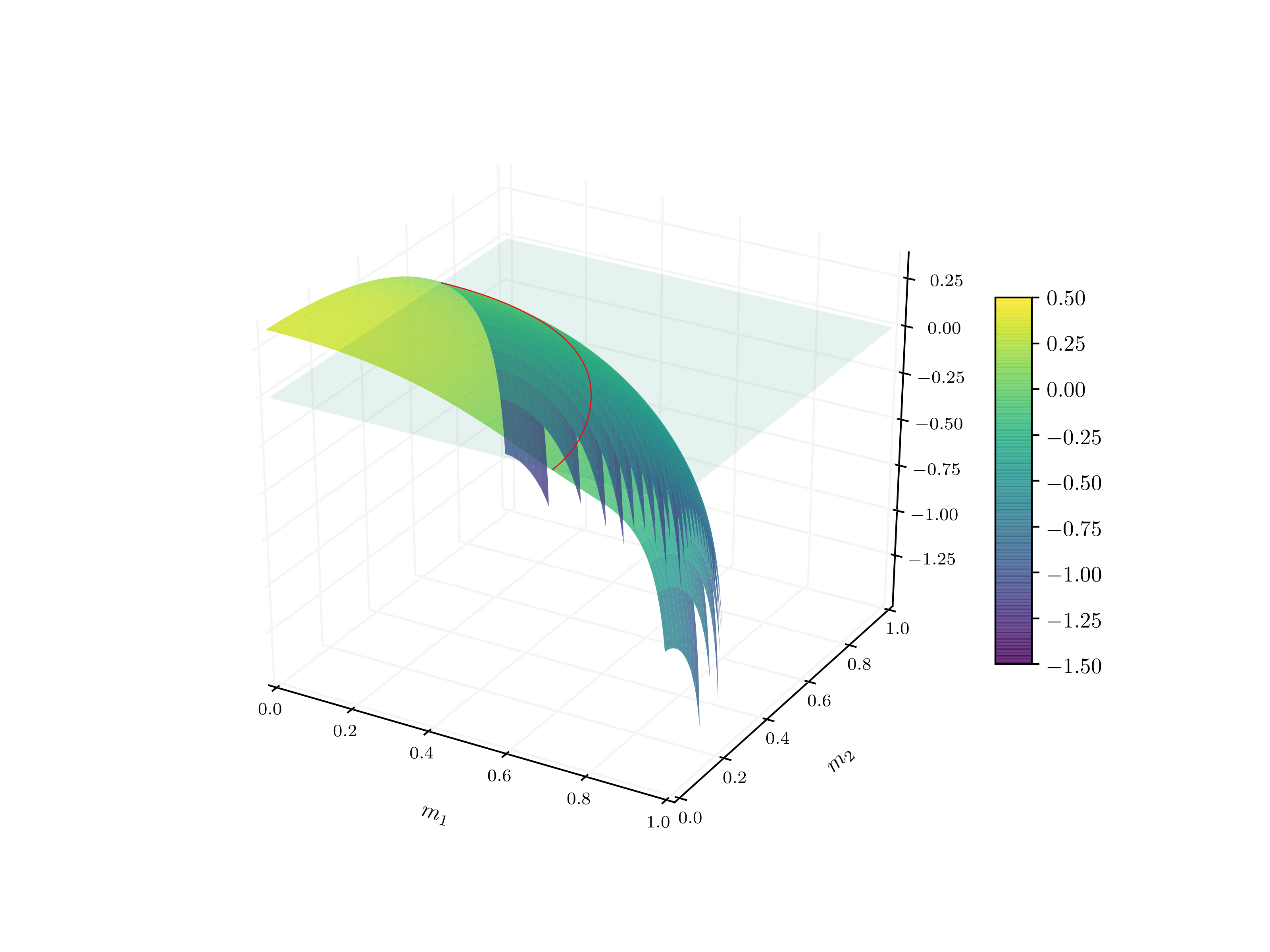
(a) $\lambda_{1}=0.5$ and $\lambda_{2}=0.2$.

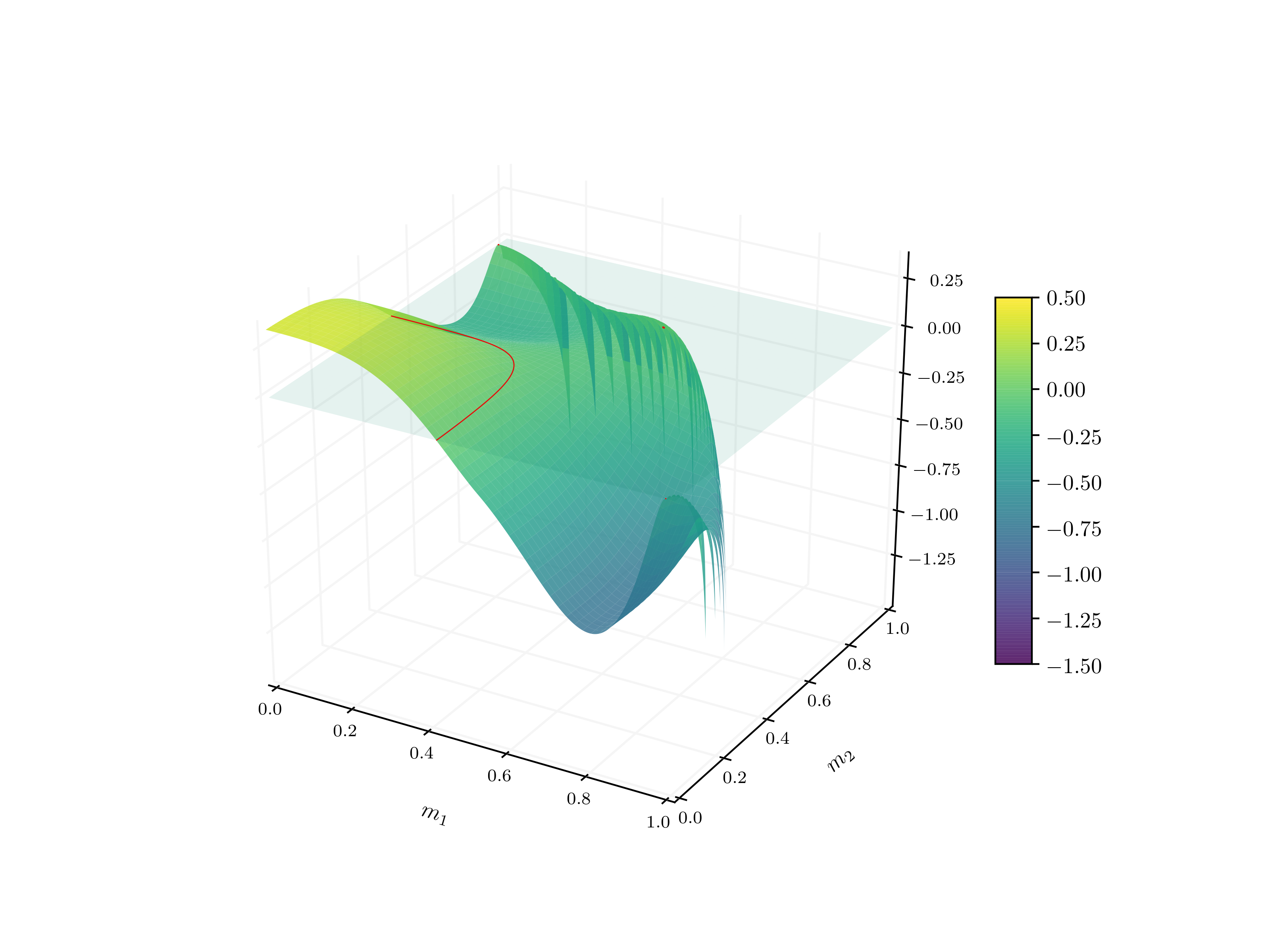
(b) $\lambda_{1}=2$ and $\lambda_{2}=1.5$.

Figure 1. 3D plots of $\Sigma^{\text{tot}}(\bm{m})$ when $r=2$ and $k=p=3$ for different values of $\lambda_{1}$ and $\lambda_{2}$. The regions where $\Sigma^{\text{tot}}(\bm{m})$ vanishes are in red. For sufficiently large values of $m_{1}$ and $m_{2}$, complexity is negative on the left, while on the right, complexity vanishes for $(m_{1},m_{2})\approx(1,0)$, $(m_{1},m_{2})\approx(0,1)$, and for large values of both $m_{1},m_{2}$ such that $m_{2}\geq m_{1}>0$.

The next result identifies the topological phase transition for large values of $m_{1},\ldots,m_{r}$.

Theorem 2.8.

We assume that $k_{i}=k$ for all $1\leq i\leq r$ and that $\bm{m}=(m_{1},\ldots,m_{r})\in D_{\Sigma}$ with $D_{\Sigma}\subset[0,1]^{r}$. We introduce the parameters $\tau(\bm{m}),\eta(\bm{m})$ and the critical values $\tau_{\textnormal{c}},\eta_{\textnormal{c}}$ by

$$\tau(\bm{m})\coloneqq\frac{k}{p}\sum_{i=1}^{r}\lambda_{i}m_{i}^{k}\quad\text{and}\quad\tau_{\textnormal{c}}\coloneqq\frac{p-2}{\sqrt{2p(p-1)}},$$

and

$$\eta(\bm{m})\coloneqq\sum_{i=1}^{r}\lambda_{i}^{-\frac{2}{k-2}}\mathbf{1}_{\{m_{i}\neq 0\}}\quad\text{and}\quad\eta_{\textnormal{c}}\coloneqq(k-2)\left(\frac{2k^{2}}{p(k-1)^{(k-1)}}\right)^{\frac{1}{k-2}},$$

respectively. Then, for $\tau(\bm{m})\geq\tau_{\textnormal{c}}$, the complexity function $\Sigma^{\text{tot}}(\bm{m})$ admits a continuous phase transition in $\eta(\bm{m})$:

• if $\eta(\bm{m})>\eta_{\textnormal{c}}$, then $\Sigma^{\text{tot}}(\bm{m})<0$,

• if $\eta(\bm{m})\leq\eta_{\textnormal{c}}$, then $\Sigma^{\text{tot}}(\bm{m})\leq 0$ and vanishes whenever $\bm{m}$ satisfies

  $$\lambda_{i}m_{i}^{k-2}=\lambda_{j}m_{j}^{k-2}\quad\text{for all}\enspace 1\leq i,j\leq r\enspace\text{such that}\enspace m_{i},m_{j}\neq 0,$$ (2.15)

  and

  $$\frac{k}{p}\sum_{i=1}^{r}\lambda_{i}m_{i}^{k}=\frac{1}{\sqrt{2p}}\frac{\sum_{i=1}^{r}m_{i}^{2}}{\sqrt{1-\sum_{i=1}^{r}m_{i}^{2}}}.$$ (2.16)

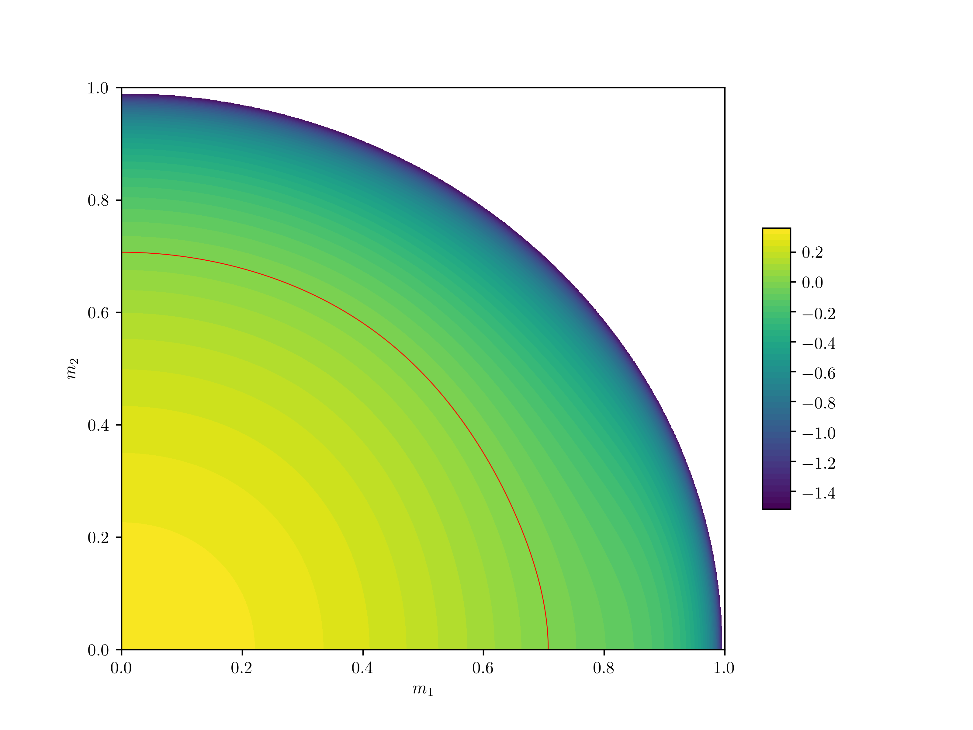
(a) $\lambda_{1}=0.5$ and $\lambda_{2}=0.2$.

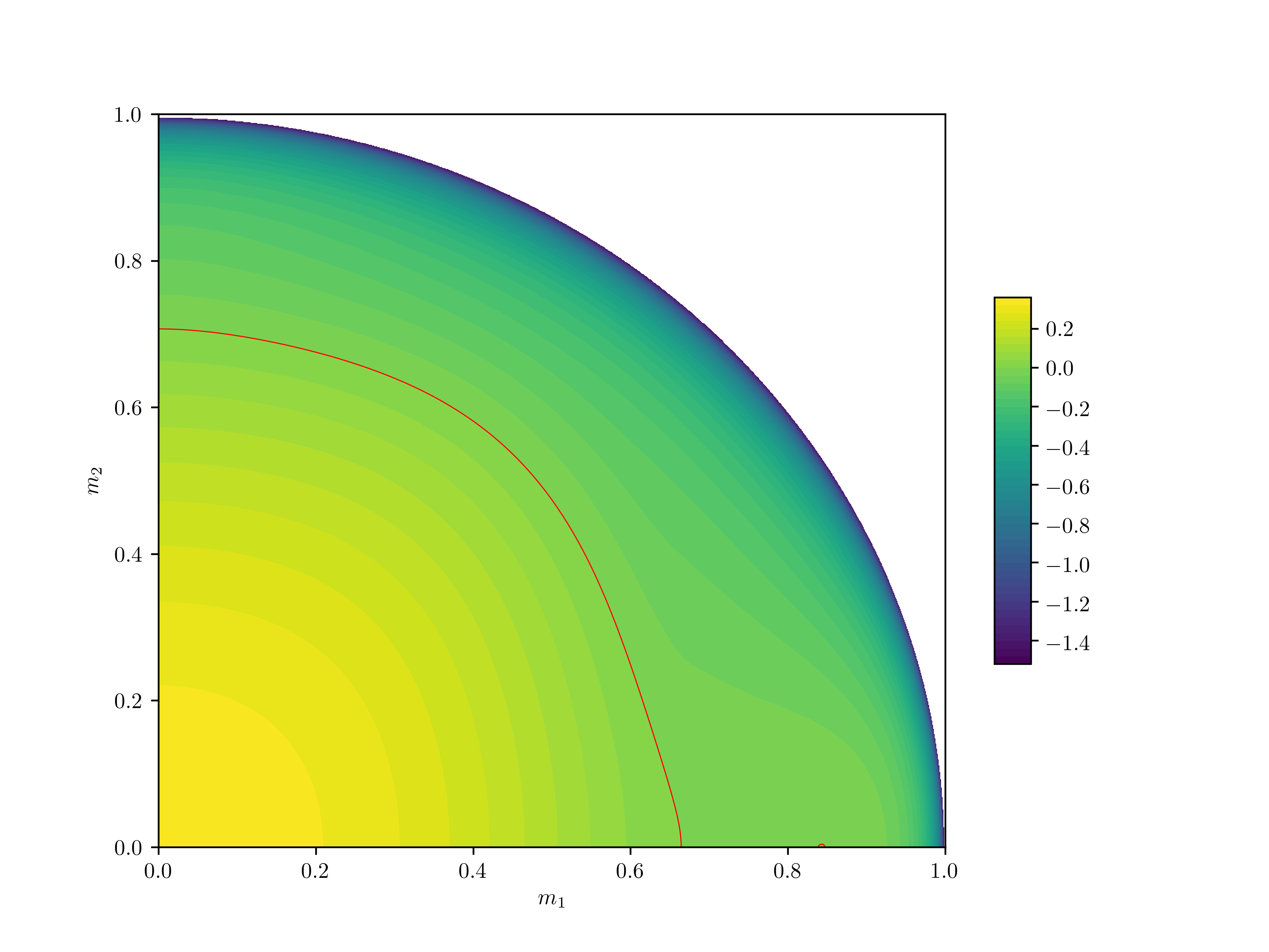
(b) $\lambda_{1}=0.9$ and $\lambda_{2}=0.5$.

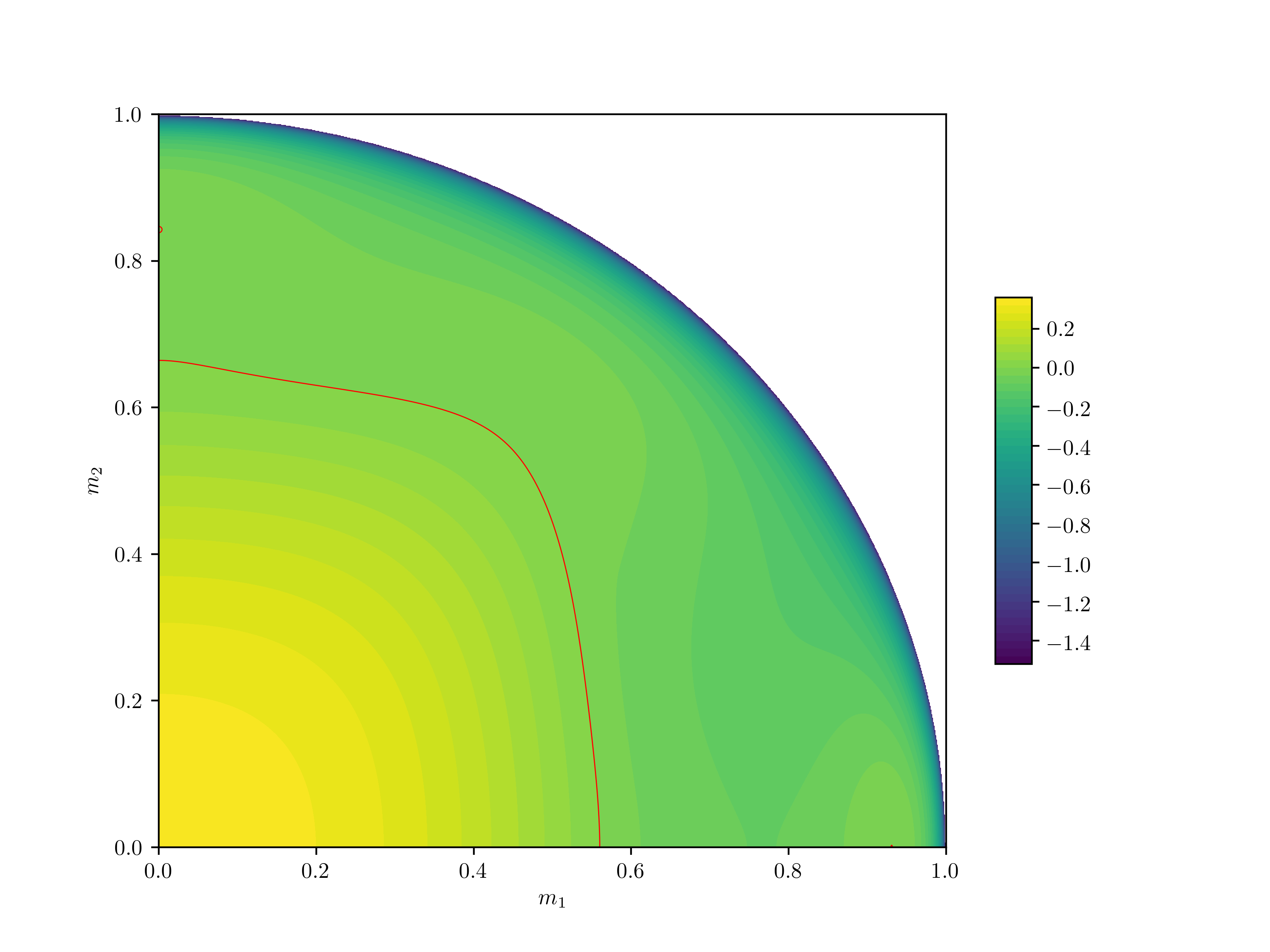
(c) $\lambda_{1}=1.2$ and $\lambda_{2}=0.9$.

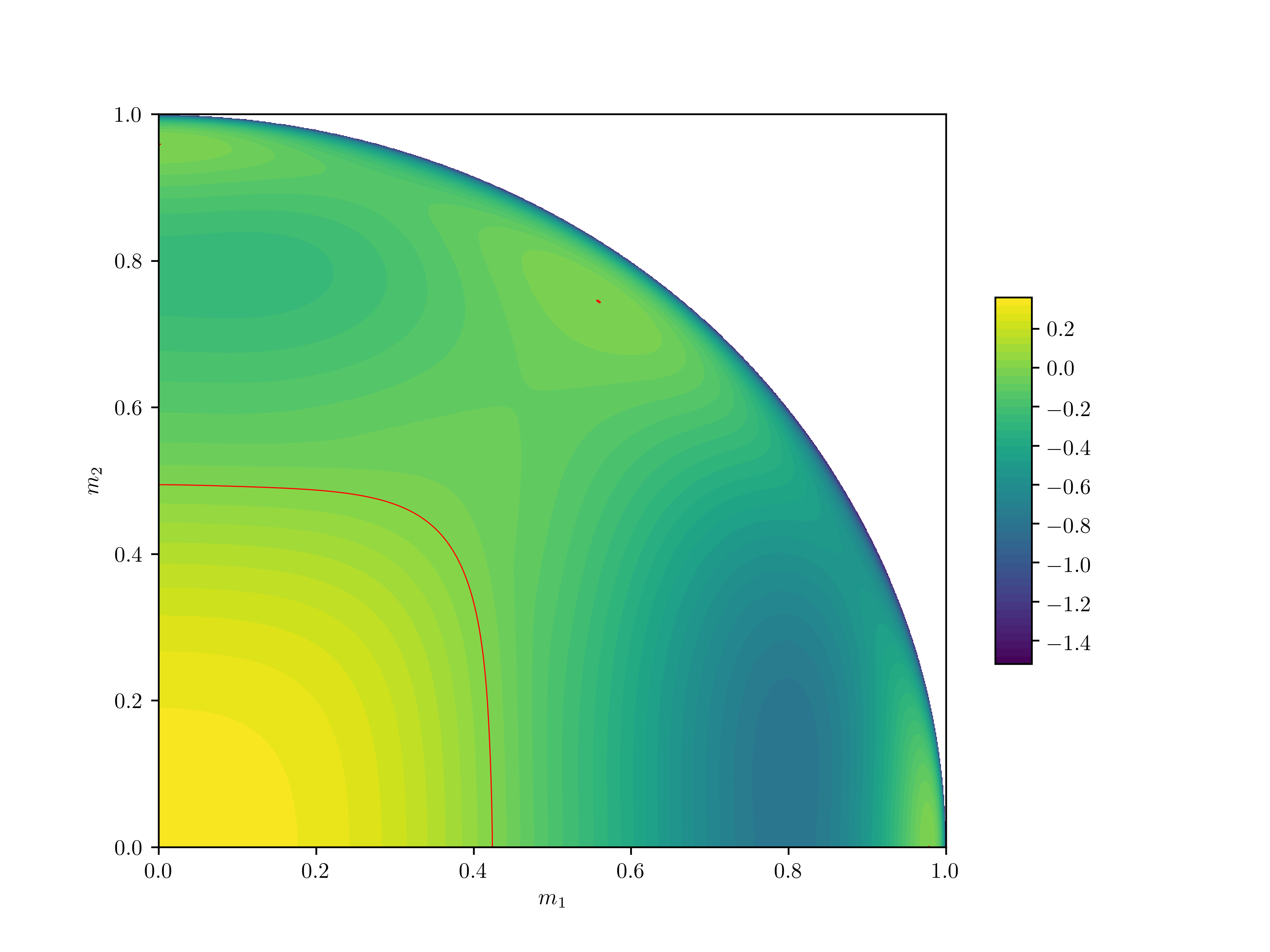
(d) $\lambda_{1}=2$ and $\lambda_{2}=1.5$.

Figure 2. Contour plots of $\Sigma^{\textnormal{tot}}(\bm{m})$ when $r=2$ and $k=p=3$ for different values of $\lambda_{1}$ and $\lambda_{2}$. The regions where $\Sigma^{\text{tot}}(\bm{m})$ vanishes are in red.

The proof of Theorem 2.8 is given in Section 5. Theorem 2.8 reduces to Proposition 2 of [15] in the case of the spiked tensor model. In particular, when $r=1$ and $k=p$, there is a critical value $\lambda_{c}$,

$$\lambda_{\text{c}}=\sqrt{\frac{1}{2p}\frac{(p-1)^{(p-1)}}{(p-2)^{(p-2)}}},$$

such that when $\lambda<\lambda_{c}$, most critical values are uninformative since they have a small scalar product with the true signal $\bm{u}^{\ast}$, while when $\lambda>\lambda_{c}$, it is possible to identify good critical points that are close to the given vector. According to Theorem 2.8, we find a similar qualitative picture when $r\geq 2$ that we describe in the following for $r=2$ (this can be generalized for $r\geq 3$).

1. When $\lambda_{\text{c}}>\lambda_{1}\geq\lambda_{2}$, there is a band with a sub-exponential number of critical points which have small values of $m_{1},m_{2}$, as shown in Figures 1(a) and 2(a).

2. When $\lambda_{1}>\lambda_{\text{c}}>\lambda_{2}$, there is a new region where complexity vanishes, characterized by $m_{2}\approx 0$ and $m_{1}$ large (see Figure 2(b)). The critical points of this new region have large scalar product with the vector $\bm{u}^{\ast}_{1}$.

3. When $\lambda_{1}\geq\lambda_{2}>\lambda_{\text{c}}$ and $\lambda_{1}^{-2/(k-2)}+\lambda_{2}^{-2/(k-2)}>\eta_{\text{c}}$, we identify a new region of zero complexity, characterized by $m_{1}\approx 0$ and $m_{2}$ large (see Figure 2(c)). In this regime, we find critical points that are close either to $\bm{u}^{\ast}_{1}$ or to $\bm{u}^{\ast}_{2}$.

4. When $\lambda_{1}\geq\lambda_{2}>\lambda_{\text{c}}$ and $\lambda_{1}^{-2/(k-2)}+\lambda_{2}^{-2/(k-2)}\leq\eta_{\text{c}}$, as illustrated in Figures 1(b) and 2(d), we find an additional region where complexity vanishes. Here, the critical points are close to both vectors $\bm{u}^{\ast}_{1}$ and $\bm{u}^{\ast}_{2}$.

Our main finding concerns regions of zero complexity in which critical points have a large scalar product with multiple spikes, as described by (4), and generalizes the phenomenon observed in [15] in the case of a single spike. These new regions are characterized by large values of $m_{1},\ldots,m_{r}$ such that $m_{r}\geq\cdots\geq m_{2}\geq m_{1}$. Indeed, by Theorem 2.8, for $m_{1},\ldots,m_{r}\neq 0$ we have that $\Sigma^{\textnormal{tot}}(\bm{m})=0$ whenever $\lambda_{1}m_{1}^{p-2}=\lambda_{2}m_{2}^{p-2}=\ldots=\lambda_{r}m_{r}^{p-2}$, and since by assumption $\lambda_{1}\geq\lambda_{2}\geq\cdots\geq\lambda_{r}$, it then follows that $0<m_{1}\leq m_{2}\leq\cdots\leq m_{r}$.

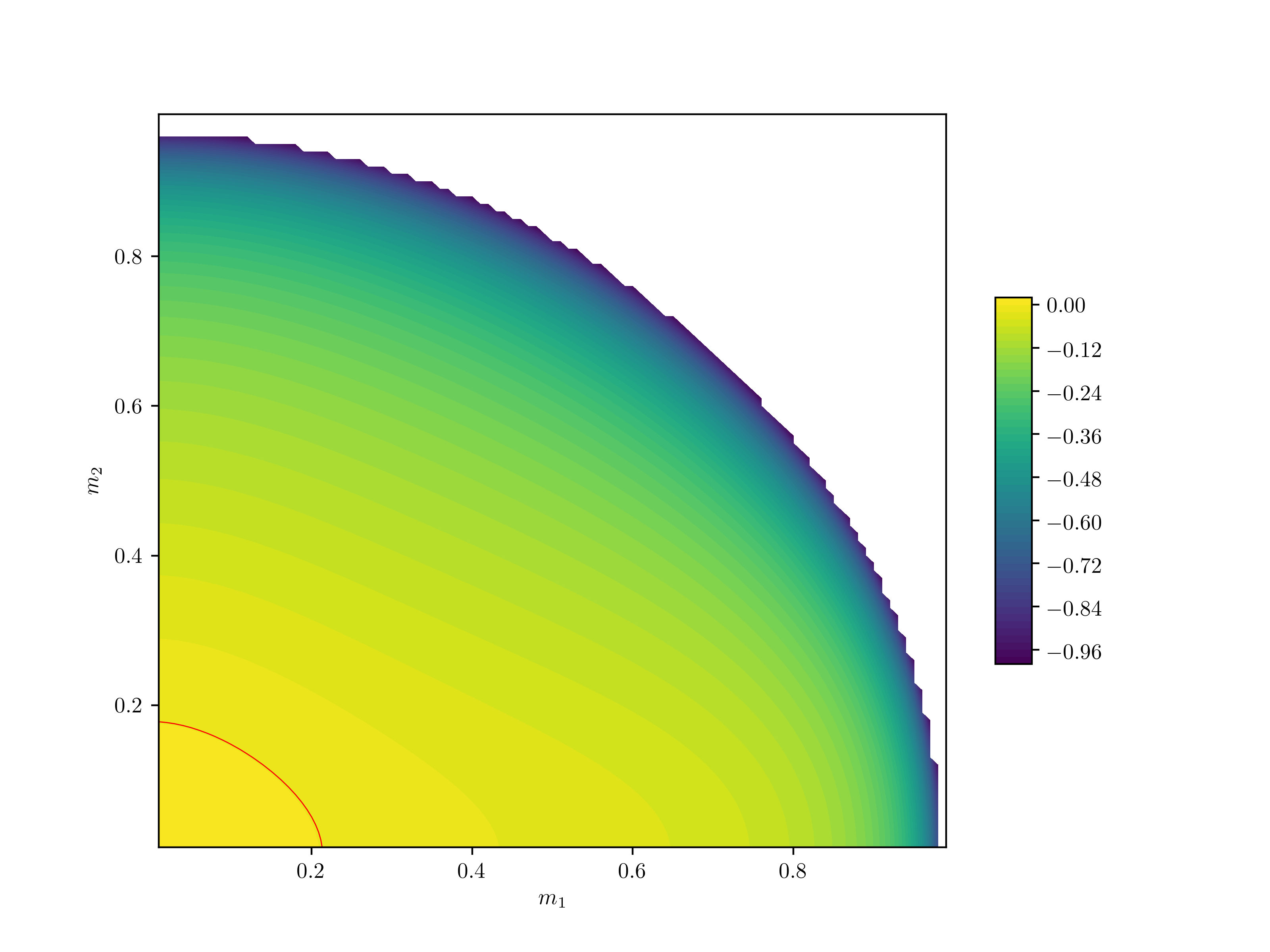
(a) $\lambda_{1}=0.5$ and $\lambda_{2}=0.2$.

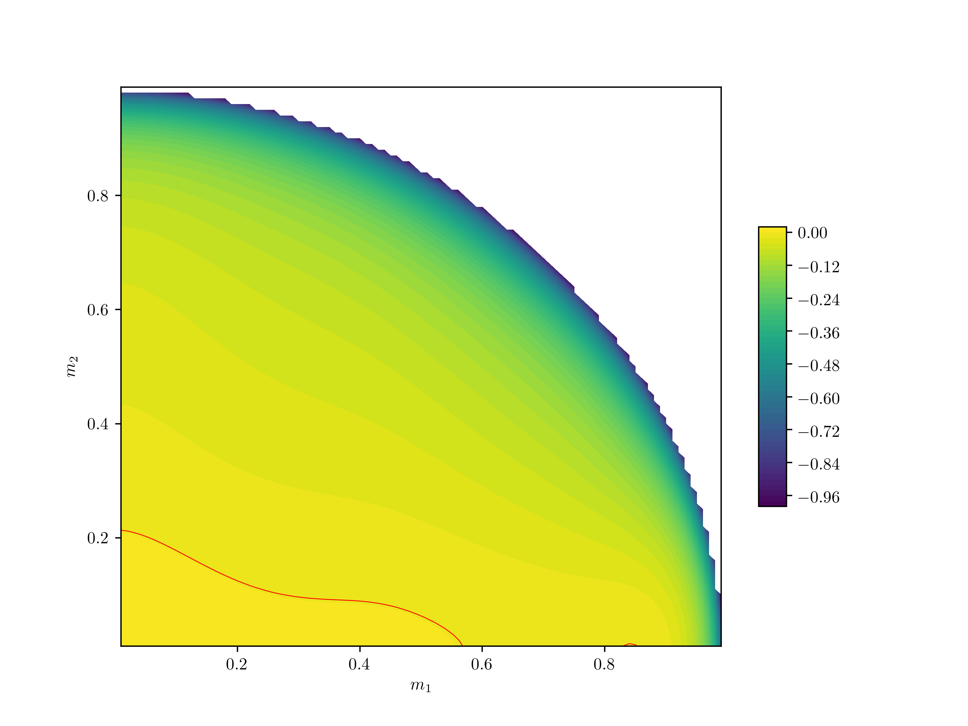
(b) $\lambda_{1}=0.9$ and $\lambda_{2}=0.5$.

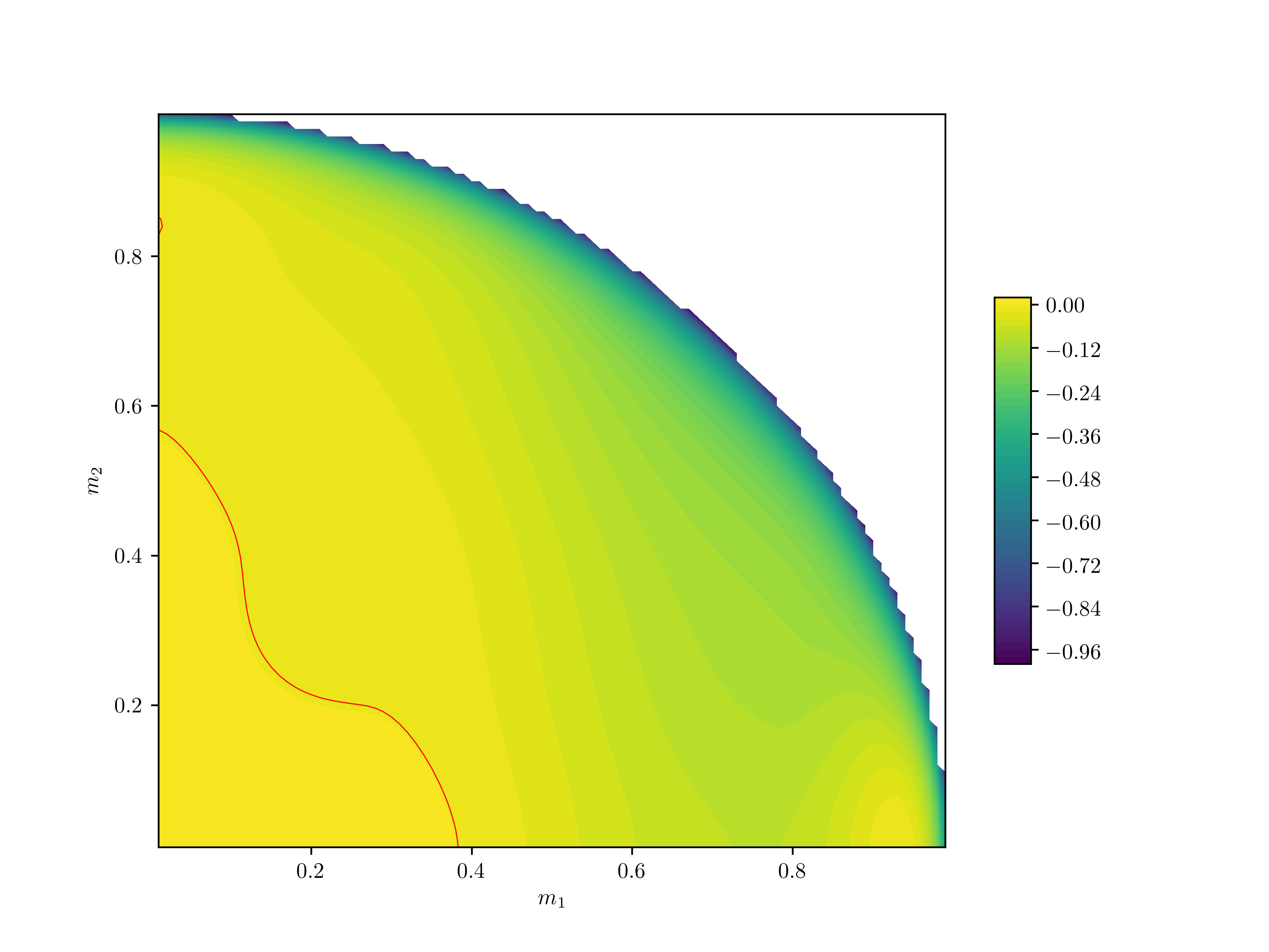
(c) $\lambda_{1}=1.2$ and $\lambda_{2}=0.9$.

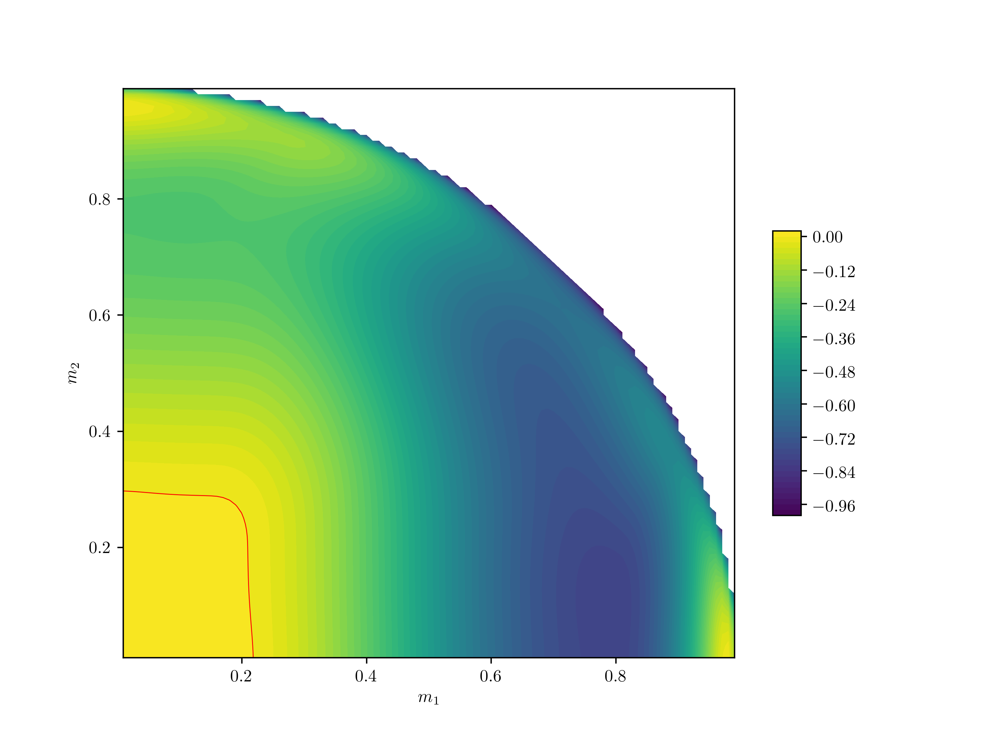
(d) $\lambda_{1}=2$ and $\lambda_{2}=1.5$.

Figure 3. Contour plots of $\Sigma^{\textnormal{tot}}(\bm{m})$ when $r=2$ and $k=p=3$ for different values of $\lambda_{1}$ and $\lambda_{2}$. The regions where $\Sigma^{\text{tot}}(\bm{m})$ vanishes are in red.

Next we focus on the variational problem of Theorem 2.7 and we consider the complexity function $\Sigma^{\textnormal{max}}(\bm{m})$ with $\bm{m}\in D_{\Sigma}\subset[0,1]^{r}$. We numerically characterize $\Sigma^{\textnormal{max}}(\bm{m})$ for $r=2$ and we find a qualitative picture similar to that of critical points. In this case, the non-zero eigenvalues $\gamma_{1}(\bm{m})$ and $\gamma_{2}(\bm{m})$ of $P_{N-1}(\bm{m})$ are given by

$$\gamma_{1,2}(\bm{m})=\frac{1}{2}\left(\theta_{1}(m_{1})+\theta_{2}(m_{2})\pm\sqrt{(\theta_{1}(m_{1})-\theta_{2}(m_{2}))^{2}+4\theta_{1}(m_{1})\theta_{2}(m_{2})\langle v_{1}(\bm{m}),v_{2}(\bm{m})\rangle^{2}}\right),$$

where $\theta_{1}(m_{1})$ and $\theta_{2}(m_{2})$ are defined by (2.10) and $\langle v_{1}(\bm{m}),v_{2}(\bm{m})\rangle$ by (2.11). Since we consider here $D_{\Sigma}\subset[0,1]^{r}$, we have that $P_{N-1}=VD_{\theta}V^{\top}$ is a positive semi-definite matrix so that $\gamma_{1}(\bm{m})\geq\gamma_{2}(\bm{m})\geq 0$ for any values of $\bm{m}\in D_{\Sigma}$. As illustrated in Figure 3, when $\lambda_{1}>\lambda_{\text{c}}>\lambda_{2}$, we find a new region where complexity vanishes, characterized by $m_{2}\approx 0$ and $m_{1}$ very large. The local maxima of this region are therefore close to $\bm{u}_{1}^{\ast}$. Similarly, as $\lambda_{2}$ crosses the critical threshold $\lambda_{\text{c}}$, then complexity also vanishes for $m_{1}\approx 0$ and $m_{2}$ very large. These local maxima are close to $\bm{u}_{2}^{\ast}$. Unlike in the case of total critical points, it is worth noting that the region of zero complexity characterized by critical points that are close with both spikes $\bm{u}_{1}^{\ast}$ and $\bm{u}_{2}^{\ast}$ is not observed in the case of local maxima. This suggests that critical points which are close to more than one given vector are probably saddle points.

3. Background

In this section, we state all the preliminary results that will be used throughout the paper. In particular, in Subsection 3.1 we characterize the complexity of the landscape for all integers $N$ via the Kac-Rice formula and in Subsection 3.2 we provide the large deviations for the largest eigenvalue of a finite-rank spiked GOE matrix. We recall that an $N\times N$ matrix $W_{N}$ in the Gaussian Orthogonal Ensemble (GOE), $W_{N}\sim\text{GOE}(N)$, is a real symmetric matrix, whose entries are independent up to symmetry, with Gaussian distribution of mean zero and variance $\mathbf{E}\left[(W_{N})_{ij}^{2}\right]=\frac{1+\delta_{ij}}{2N}$.

3.1. Kac-Rice formula and landscape complexity

The Kac-Rice formula is the classical technique to compute the average number of critical points of a real-valued Gaussian random function on $\mathbb{R}^{N}$. In particular, we apply here Theorem 12.1.1 and Corollary 12.1.2 of [1] to the random function $f_{N}$ introduced in (1.2). We refer the reader to [1, 7] for a broader introduction on the Kac-Rice method.

Lemma 3.1 (Kac-Rice formula [1]).

For every Borel sets $M_{1},\ldots,M_{r}\subset[-1,1]$, $B\subset\mathbb{R}$ and for all $N$, it holds that

$$\begin{split}\mathbf{E}\left[\textnormal{Crt}_{N}^{\textnormal{tot}}((M_{i})_{i=1}^{r},B)\right]&=\int_{\{\bm{\sigma}\colon\langle\bm{\sigma},\bm{u}_{i}^{\ast}\rangle\in M_{i},\,\forall\,1\leq i\leq r\}}\textnormal{d}\bm{\sigma}\,\varphi_{\nabla_{\mathbb{S}^{N-1}}f_{N}(\bm{\sigma})}(\bm{0})\\ &\quad\times\mathbf{E}\left[\left|\det\left(\nabla_{\mathbb{S}^{N-1}}^{2}f_{N}(\bm{\sigma})\right)\right|\cdot\mathbf{1}_{\{f_{N}(\bm{\sigma})\in B\}}|\nabla_{\mathbb{S}^{N-1}}f_{N}(\bm{\sigma})=\bm{0}\right],\end{split}$$ (3.1)

and for every $0\leq\ell\leq N-1$,

$$\begin{split}\mathbf{E}\left[\textnormal{Crt}_{N}^{\ell}((M_{i})_{i=1}^{r},B)\right]&=\int_{\{\bm{\sigma}\colon\langle\bm{\sigma},\bm{u}_{i}^{\ast}\rangle\in M_{i},\,\forall\,1\leq i\leq r\}}\textnormal{d}\bm{\sigma}\,\varphi_{\nabla_{\mathbb{S}^{N-1}}f_{N}(\bm{\sigma})}(\bm{0})\\ &\quad\times\mathbf{E}\left[\left|\det\left(\nabla_{\mathbb{S}^{N-1}}^{2}f_{N}(\bm{\sigma})\right)\right|\cdot\mathbf{1}_{\left\{i(\nabla_{\mathbb{S}^{N-1}}^{2}f_{N}(\bm{\sigma}))=\ell,\,f_{N}(\bm{\sigma})\in B\right\}}|\nabla_{\mathbb{S}^{N-1}}f_{N}(\bm{\sigma})=\bm{0}\right],\end{split}$$ (3.2)

where $\text{d}\bm{\sigma}$ denotes the usual surface measure on $\mathbb{S}^{N-1}$, and $\varphi_{\nabla_{\mathbb{S}^{N-1}}f_{N}(\bm{\sigma})}(\bm{0})$ denotes the density of $\nabla_{\mathbb{S}^{N-1}}f_{N}(\bm{\sigma})$ evaluated at $\bm{0}$.

Given Borel sets $M_{1},\ldots,M_{r}\subset[-1,1]$, we let $M=M_{1}\times\cdots\times M_{r}$. In the following, to simplify notation, we write $\textnormal{Crt}_{N}^{\textnormal{tot}}(M,B)$ and $\textnormal{Crt}_{N}^{\ell}(M,B)$ for the random variables given by (2.1) and (2.2), respectively. We recall the definition of the set $D_{\Sigma}=\left\{\bm{m}=(m_{1},\ldots,m_{r})\in M\colon\sum_{i=1}^{r}m_{i}^{2}<1\right\}\subset[-1,1]^{r}$. We next introduce the function $S(\bm{m},x)$, which is $-\infty$ in $D_{\Sigma}^{\text{c}}\times\mathbb{R}$, and in $D_{\Sigma}\times\mathbb{R}$ is given by

$$\begin{split}S(\bm{m},x)&=\frac{1}{2}(\log(p-1)+1)+\frac{1}{2}\log\left(1-\sum_{i=1}^{r}m_{i}^{2}\right)-\frac{1}{p}\sum_{i=1}^{r}\lambda_{i}^{2}k_{i}^{2}m_{i}^{2k_{i}-2}(1-m_{i}^{2})\\ &\quad+\frac{2}{p}\sum_{1\leq i<j\leq r}\lambda_{i}\lambda_{j}k_{i}k_{j}m_{i}^{k_{i}}m_{j}^{k_{j}}-\left(x-\sum_{i=1}^{r}\lambda_{i}m_{i}^{k_{i}}\right)^{2}.\end{split}$$ (3.3)

The following result provides the characterization of the landscape complexity for all integers $N$.

Proposition 3.2 (Landscape complexity).

For every Borel sets $M_{1},\ldots,M_{r}\subset[-1,1]$, $B\subset\mathbb{R}$ and for all $N$, it holds that

$$\begin{split}&\mathbf{E}\left[\textnormal{Crt}_{N}^{\textnormal{tot}}(M,B)\right]\\ &=C_{N}\int_{B}\textnormal{d}x\int_{M_{1}}\textnormal{d}m_{1}\,\dots\int_{M_{r}}\textnormal{d}m_{r}\,\left(1-\sum_{i=1}^{r}m_{i}^{2}\right)^{-\frac{r+2}{2}}\exp\{NS(\bm{m},x)\}\mathbf{E}\left[|\det H_{N-1}(\bm{m},x)|\right],\end{split}$$ (3.4)

and for every $0\leq\ell\leq N-1$,

$$\begin{split}\mathbf{E}\left[\textnormal{Crt}_{N}^{\ell}(M,B)\right]&=C_{N}\int_{B}\textnormal{d}x\int_{M_{1}}\textnormal{d}m_{1}\,\dots\int_{M_{r}}\textnormal{d}m_{r}\,\left(1-\sum_{i=1}^{r}m_{i}^{2}\right)^{-\frac{r+2}{2}}\exp\{NS(\bm{m},x)\}\\ &\quad\times\mathbf{E}\left[|\det H_{N-1}(\bm{m},x)|\cdot\mathbf{1}_{\{i(H_{N-1}(\bm{m},x))=\ell\}}\right].\end{split}$$ (3.5)

Here, $H_{N-1}(\bm{m},x)$ is an $(N-1)$-dimensional square random matrix distributed as

$$H_{N-1}(\bm{m},x)\stackrel{{\scriptstyle d}}{{=}}W_{N-1}+\sqrt{\frac{N}{N-1}}P_{N-1}(\bm{m})-\sqrt{\frac{N}{N-1}}t(\bm{m},x)I_{N-1},$$ (3.6)

where $W_{N-1}\sim\textnormal{GOE}(N-1)$, $P_{N-1}(\bm{m})$ is given by Definition 2.5 and the function $t(\bm{m},x)$ by (2.12). Moreover, the constant $C_{N}=C(N,r,p)$ is exponentially trivial, meaning that $\lim_{N\to\infty}\frac{1}{N}\log C_{N}=0$.

We prove Proposition 3.2 using the Kac-Rice formula (see Lemma 3.1) and the following result which provides the joint law of the Gaussian random variables $(f_{N}(\bm{\sigma}),\nabla_{\mathbb{S}^{N-1}}f_{N}(\bm{\sigma}),\nabla_{\mathbb{S}^{N-1}}^{2}f_{N}(\bm{\sigma}))$.

Lemma 3.3.

For every Borel sets $M_{1},\ldots,M_{r}\subset[-1,1]$, $B\subset\mathbb{R}$ and for all $N$, it holds that

$$\begin{split}\mathbf{E}\left[\textnormal{Crt}_{N}^{\textnormal{tot}}(M,B)\right]&=\omega_{N-r}\int_{M_{1}}\textnormal{d}m_{1}\,\dots\int_{M_{r}}\textnormal{d}m_{r}\,\varphi_{\nabla_{\mathbb{S}^{N-1}}f_{N}(\bm{\sigma})}(\bm{0})\left(1-\sum_{i=1}^{r}m_{i}^{2}\right)^{\frac{N-r-2}{2}}\\ &\quad\times\mathbf{E}\left[|\det\nabla_{\mathbb{S}^{N-1}}^{2}f_{N}(\bm{\sigma})|\cdot\mathbf{1}_{\{f_{N}(\bm{\sigma})\in B\}}\right],\end{split}$$ (3.7)

and for every $0\leq\ell\leq N-1$,

$$\begin{split}\mathbf{E}\left[\textnormal{Crt}_{N}^{\ell}(M,B)\right]&=\omega_{N-r}\int_{M_{1}}\textnormal{d}m_{1}\,\dots\int_{M_{r}}\textnormal{d}m_{r}\,\varphi_{\nabla_{\mathbb{S}^{N-1}}f_{N}(\bm{\sigma})}(\bm{0})\left(1-\sum_{i=1}^{r}m_{i}^{2}\right)^{\frac{N-r-2}{2}}\\ &\quad\times\mathbf{E}\left[|\det\nabla_{\mathbb{S}^{N-1}}^{2}f_{N}(\bm{\sigma})|\cdot\mathbf{1}_{\left\{i(\nabla_{\mathbb{S}^{N-1}}^{2}f_{N}(\bm{\sigma}))=\ell\right\}}\cdot\mathbf{1}_{\{f_{N}(\bm{\sigma})\in B\}}\right],\end{split}$$ (3.8)

where $\omega_{N}=\frac{2\pi^{N/2}}{\Gamma(N/2)}$ is the volume of the $(N-1)$-dimensional unit sphere. Further, the joint distribution of $f_{N}(\bm{\sigma})\in\mathbb{R}$, $\nabla_{\mathbb{S}^{N-1}}f_{N}(\bm{\sigma})\in\mathbb{R}^{N-1}$ and $\nabla_{\mathbb{S}^{N-1}}^{2}f_{N}(\bm{\sigma})\in\mathbb{R}^{(N-1)\times(N-1)}$ is given by

$$\begin{split}f_{N}(\bm{\sigma})&\stackrel{{\scriptstyle d}}{{=}}\sum_{i=1}^{r}\lambda_{i}m_{i}^{k_{i}}+\frac{1}{\sqrt{2N}}Z,\\ \nabla_{\mathbb{S}^{N-1}}f_{N}(\bm{\sigma})&\stackrel{{\scriptstyle d}}{{=}}\sum_{i=1}^{r}\lambda_{i}k_{i}m_{i}^{k_{i}-1}\sqrt{1-m_{i}^{2}}\bm{v}_{i}(\bm{m})+\sqrt{\frac{p}{2N}}\bm{g}_{N-1},\\ \nabla_{\mathbb{S}^{N-1}}^{2}f_{N}(\bm{\sigma})&\stackrel{{\scriptstyle d}}{{=}}\sum_{i=1}^{r}\lambda_{i}k_{i}(k_{i}-1)m_{i}^{k_{i}-2}(1-m_{i}^{2})\bm{v}_{i}(\bm{m})\bm{v}_{i}(\bm{m})^{\top}+\sqrt{\frac{p(p-1)(N-1)}{2N}}W_{N-1}\\ &\quad-\left(\sum_{i=1}^{r}\lambda_{i}k_{i}m_{i}^{k_{i}}+\frac{p}{\sqrt{2N}}Z\right)I_{N-1},\end{split}$$ (3.9)

where $Z\sim\mathcal{N}(0,1)$, $\bm{g}_{N-1}\sim\mathcal{N}(0,I_{N-1})$, $W_{N-1}\sim\textnormal{GOE}(N-1)$ are independent, and for each $1\leq i\leq r$, the vector-valued function $\bm{v}_{i}(\bm{m})\in\mathbb{S}^{N-2}$ is defined by (2.11). Here, we identified the tangent space $\text{T}_{\bm{\sigma}}\mathbb{S}^{N-1}$ with $\mathbb{R}^{N-1}$.

Having Lemma 3.3 at hand, we turn to the proof of Proposition 3.2.

Proof of Proposition 3.2.

According to (3.9), we have that $f_{N}$ is distributed as a Gaussian random variable with mean $\sum_{i=1}^{r}\lambda_{i}m_{i}^{k_{i}}$ and variance $\frac{1}{2N}$, hence the density function $p_{f_{N}}$ is given by

$$p_{f_{N}}(x)=\sqrt{\frac{N}{\pi}}\exp\left\{-N\left(x-\sum_{i=1}^{r}\lambda_{i}m_{i}^{k_{i}}\right)^{2}\right\}.$$ (3.10)

Therefore, the inner expectation in (3.8) can be expanded as

$$\begin{split}&\mathbf{E}\left[|\det\nabla_{\mathbb{S}^{N-1}}^{2}f_{N}(\bm{\sigma})|\cdot\mathbf{1}_{\left\{i(\nabla_{\mathbb{S}^{N-1}}^{2}f_{N}(\bm{\sigma}))=\ell\right\}}\cdot\mathbf{1}_{\{f_{N}(\bm{\sigma})\in B\}}\right]\\ &=\left(\frac{p(p-1)(N-1)}{2N}\right)^{\frac{N-1}{2}}\int_{B}\mathbf{E}\left[|\det H_{N-1}(\bm{m},x)|\cdot\mathbf{1}_{\{i(H_{N-1}(\bm{m},x))=\ell\}}\right]p_{f_{N}}(x)\text{d}x,\end{split}$$ (3.11)

where the matrix $H_{N-1}(\bm{m},x)$ is distributed as in (3.6). Further, the random vector $\nabla_{\mathbb{S}^{N-1}}f_{N}(\bm{\sigma})$ is Gaussian with mean $\sum_{i=1}^{r}\lambda_{i}k_{i}m_{i}^{k_{i}-1}\sqrt{1-m_{i}^{2}}\bm{v}_{i}(\bm{m})$ and covariance matrix $\frac{p}{2N}I_{N-1}$, thus its density function at $\bm{0}$ is given by

$$\varphi_{\nabla_{\mathbb{S}^{N-1}}f_{N}(\bm{\sigma})}(\bm{0})=\left(\frac{N}{\pi p}\right)^{\frac{N-1}{2}}\exp\left\{-\frac{N}{p}\sum_{i=1}^{r}\lambda_{i}^{2}k_{i}^{2}m_{i}^{2k_{i}-2}(1-m_{i}^{2})+\frac{2N}{p}\sum_{1\leq i<j\leq r}\lambda_{i}\lambda_{j}k_{i}k_{j}m_{i}^{k_{i}}m_{j}^{k_{j}}\right\}.$$ (3.12)

Plugging (3.10)-(3.12) into (3.8), we obtain that

$$\begin{split}&\mathbf{E}\left[\textnormal{Crt}_{N}^{\ell}(M,B)\right]\\ &=\left(\frac{p(p-1)(N-1)}{2N}\right)^{\frac{N-1}{2}}\omega_{N-r}\int_{M_{1}}\text{d}m_{1}\,\ldots\int_{M_{r}}\text{d}m_{r}\,\varphi_{\nabla_{\mathbb{S}^{N-1}}f_{N}(\bm{\sigma})}(\bm{0})\left(1-\sum_{i=1}^{r}m_{i}^{2}\right)^{\frac{N-r-2}{2}}\\ &\quad\times\int_{B}\text{d}x\,\mathbf{E}\left[|\det{H}_{N-1(\bm{m},x)}|\cdot\mathbf{1}_{\{i(H_{N-1}(\bm{m},x))=\ell\}}\right]p_{f_{N}}(x)\\ &=C_{N}\int_{B}\text{d}x\int_{M_{1}}\text{d}m_{1}\,\dots\int_{M_{r}}\text{d}m_{r}\,\left(1-\sum_{i=1}^{r}m_{i}^{2}\right)^{-\frac{r+2}{2}}\\ &\quad\times\mathbf{E}\left[|\det H_{N-1}(\bm{m},x)|\cdot\mathbf{1}_{\{i(H_{N-1}(\bm{m},x))=\ell\}}\right]\exp\{NS(\bm{m},x)\},\end{split}$$

where $C_{N}=C(N,r,p)$ is given by

$$C(N,r,p)=2\left(\frac{N-1}{2e}\right)^{\frac{N-1}{2}}\Gamma\left(\frac{N-r}{2}\right)^{-1}\pi^{-\frac{r-1}{2}}\left(\frac{N}{(p-1)e\pi}\right)^{1/2}.$$

This proves (3.5). Identity (3.4) follows in the same way. It is straightforward to show that $C_{N}$ is exponentially trivial by expanding the function $\Gamma$ using the Stirling’s formula. ∎

It remains to derive the random matrices appearing in the Kac-Rice formula by proving Lemma 3.3.

Proof of Lemma 3.3.

We recall the definition of $f_{N}$ given by (1.2), i.e.,

$$f_{N}(\bm{\sigma})=\sum_{i=1}^{r}\lambda_{i}\langle\bm{u}_{i}^{\ast},\bm{\sigma}\rangle^{k_{i}}+H_{N}(\bm{\sigma}),$$

where $H_{N}(\bm{\sigma})$ denotes the Hamiltonian (1.1), i.e.,

$$H_{N}(\bm{\sigma})=\frac{1}{\sqrt{2N}}\frac{1}{p!}\sum_{1\leq i_{1},\ldots,i_{p}\leq N}\sum_{\pi\in\mathfrak{S}_{p}}G^{\pi}_{i_{1},\ldots,i_{p}}\sigma_{i_{1}}\cdots\sigma_{i_{p}}.$$

We denote by $\nabla$ and $\nabla^{2}$ the Euclidean gradient and Hessian, respectively. We then have that

$$\begin{split}\nabla f_{N}(\bm{\sigma})&=\sum_{i=1}^{r}\lambda_{i}k_{i}\langle\bm{u}_{i}^{\ast},\bm{\sigma}\rangle^{k_{i}-1}\bm{u}_{i}^{\ast}+\nabla H_{N}(\bm{\sigma}),\\ \nabla^{2}f_{N}(\bm{\sigma})&=\sum_{i=1}^{r}\lambda_{i}k_{i}(k_{i}-1)\langle\bm{u}_{i}^{\ast},\bm{\sigma}\rangle^{k_{i}-2}\bm{u}_{i}^{\ast}\left(\bm{u}_{i}^{\ast}\right)^{\top}+\nabla^{2}H_{N}(\bm{\sigma}),\end{split}$$

where for any $k,\ell\in\{1,\ldots,N\}$,

$$\begin{split}\left(\nabla H_{N}(\bm{\sigma})\right)_{k}&=\frac{p}{\sqrt{2N}}\frac{1}{p!}\sum_{i_{1},\ldots,i_{p-1}}\sum_{\pi\in\mathfrak{S}_{p}}G^{\pi}_{k,i_{1},\ldots,i_{p-1}}\sigma_{i_{1}}\cdots\sigma_{i_{p-1}},\\ (\nabla^{2}H_{N}(\bm{\sigma}))_{k\ell}&=\frac{p(p-1)}{\sqrt{2N}}\frac{1}{p!}\sum_{i_{1},\ldots,i_{p-2}}\sum_{\pi\in\mathfrak{S}_{p}}G^{\pi}_{k,\ell,i_{1},\ldots,i_{p-2}}\sigma_{i_{1}}\cdots\sigma_{i_{p-2}}.\end{split}$$

The Riemannian gradient and Hessian of $f_{N}$ are then given by

$$\nabla_{\mathbb{S}^{N-1}}f_{N}(\bm{\sigma})=\text{P}^{\bot}_{\bm{\sigma}}\nabla f_{N}(\bm{\sigma}),$$

and

$$\nabla_{\mathbb{S}^{N-1}}^{2}f_{N}(\bm{\sigma})=\text{P}^{\bot}_{\bm{\sigma}}\nabla^{2}f_{N}(\bm{\sigma})\text{P}^{\bot}_{\bm{\sigma}}-\langle\bm{\sigma},\nabla f_{N}(\bm{\sigma})\rangle\text{P}^{\bot}_{\bm{\sigma}},$$

respectively, where $\text{P}_{\bm{\sigma}}^{\bot}=\mathbf{I}-\bm{\sigma}\bm{\sigma}^{\top}$ denotes the orthogonal projection from $\mathbb{R}^{N}$ onto the tangent space $\text{T}_{\bm{\sigma}}\mathbb{S}^{N-1}$. Applying these formulas yields

$$\begin{split}\nabla_{\mathbb{S}^{N-1}}f_{N}(\bm{\sigma})&=\sum_{i=i}^{r}\lambda_{i}k_{i}\langle\bm{u}_{i}^{\ast},\bm{\sigma}\rangle^{k_{i}-1}\left(\text{P}^{\bot}_{\bm{\sigma}}\bm{u}_{i}^{\ast}\right)+\text{P}^{\bot}_{\bm{\sigma}}\nabla H_{N}(\bm{\sigma}),\\ \nabla_{\mathbb{S}^{N-1}}^{2}f_{N}(\bm{\sigma})&=\sum_{i=1}^{r}\lambda_{i}k_{i}(k_{i}-1)\langle\bm{u}_{i}^{\ast},\bm{\sigma}\rangle^{k_{i}-2}\left(\text{P}^{\bot}_{\bm{\sigma}}\bm{u}_{i}^{\ast}\right)\left(\text{P}^{\bot}_{\bm{\sigma}}\bm{u}_{i}^{\ast}\right)^{\top}+\text{P}^{\bot}_{\bm{\sigma}}\nabla^{2}H_{N}(\bm{\sigma})\text{P}^{\bot}_{\bm{\sigma}}\\ &\quad-\left(\sum_{i=1}^{r}\lambda_{i}k_{i}\langle\bm{u}_{i}^{\ast},\bm{\sigma}\rangle^{k_{i}}+\langle\bm{\sigma},\nabla H_{N}(\bm{\sigma})\rangle\right)\text{P}^{\bot}_{\bm{\sigma}}.\end{split}$$

Since the joint distribution of $(f_{N}(\bm{\sigma}),\nabla_{\mathbb{S}^{N-1}}f_{N}(\bm{\sigma}),\nabla_{\mathbb{S}^{N-1}}^{2}f_{N}(\bm{\sigma}))$ is invariant with respect to $\bm{\sigma}$, we may assume without loss of generality that $\bm{\sigma}=\bm{e_{N}}=(\delta_{i,N})_{i=1}^{N}$. We then define the vector $\bm{u}_{i}^{\ast}$ by

$$\bm{u}_{i}^{\ast}=m_{i}\bm{\sigma}+\sqrt{1-m_{i}^{2}}\bm{\tilde{v}}_{i}(\bm{m})$$

such that $\bm{\tilde{v}}_{1}(\bm{m}),\ldots,\bm{\tilde{v}}_{r}(\bm{m})\in\mathbb{S}^{N-1}$, $\langle\bm{\sigma},\bm{u}_{i}^{\ast}\rangle=m_{i}$ and $\langle\bm{u}_{i}^{\ast},\bm{u}^{\ast}_{j}\rangle=\delta_{ij}$. In particular, we have that the $N$-entry of each vector $\bm{\tilde{v}}_{i}(\bm{m})$ is equal to zero and

$$\langle\bm{\tilde{v}}_{i}(\bm{m}),\bm{\tilde{v}}_{j}(\bm{m})\rangle=\begin{cases}1&\text{if}\enspace i=j\\ -\frac{m_{i}m_{j}}{\sqrt{1-m_{i}^{2}}\sqrt{1-m_{j}^{2}}}&\text{if}\enspace i\neq j\end{cases}.$$

Identifying $\text{T}_{\bm{\sigma}}\mathbb{S}^{N-1}$ with $\mathbb{R}^{N-1}$, we then obtain that

$$\begin{split}f_{N}(\bm{\sigma})&\stackrel{{\scriptstyle d}}{{=}}\sum_{i=1}^{r}\lambda_{i}m_{i}^{k_{i}}+\frac{1}{\sqrt{2N}}Z,\\ \nabla_{\mathbb{S}^{N-1}}f_{N}(\bm{\sigma})&\stackrel{{\scriptstyle d}}{{=}}\sum_{i=1}^{r}\lambda_{i}k_{i}m_{i}^{k_{i}-1}\sqrt{1-m_{i}^{2}}\bm{v}_{i}(\bm{m})+\sqrt{\frac{p}{2N}}\bm{g}_{N-1},\end{split}$$

and

$$\begin{split}\nabla_{\mathbb{S}^{N-1}}^{2}f_{N}(\bm{\sigma})&\stackrel{{\scriptstyle d}}{{=}}\sum_{i=1}^{r}\lambda_{i}k_{i}(k_{i}-1)m_{i}^{k_{i}-2}(1-m_{i}^{2})\bm{v}_{i}(\bm{m})\bm{v}_{i}(\bm{m})^{\top}+\sqrt{\frac{p(p-1)(N-1)}{2N}}W_{N-1}\\ &\quad-\left(\sum_{i=1}^{r}\lambda_{i}k_{i}m_{i}^{k_{i}}+\frac{p}{\sqrt{2N}}Z\right)I_{N-1},\end{split}$$

where $Z\sim\mathcal{N}(0,1)$, $\bm{g}_{N-1}\sim\mathcal{N}(0,\bm{I}_{N-1})$ and $W_{N-1}\sim\text{GOE}(N-1)$ are independent and the vector-valued function $\bm{v}_{i}(\bm{m})\in\mathbb{S}^{N-2}$ corresponds to $\bm{\tilde{v}}_{i}(\bm{m})$ without the $N$-th entry.

According to Lemma 3.1, the integrand in (3.1) and (3.2) depends on $\bm{\sigma}$ only through the overlap $\rho(\bm{\sigma})=(\langle\bm{\sigma},\bm{u}_{1}^{\ast}\rangle,\ldots,\langle\bm{\sigma},\bm{u}_{r}^{\ast}\rangle)$. We can then use the co-area formula with the function $\rho(\bm{\sigma})$ to express the integral as an $r$-dimensional integral over the parameters $m_{1},\ldots,m_{r}$, where $m_{i}\in M_{i}$. The volume of the inverse-image $\rho^{-1}(m_{1},\ldots,m_{r})$ is given by

$$\omega_{N-r}\left(1-\sum_{i=1}^{r}m_{i}^{2}\right)^{\frac{N-r-1}{2}},$$

and the inverse of the Jacobian is given by $\left(1-\sum_{i=1}^{r}m_{i}^{2}\right)^{-\frac{1}{2}}$. For every $0\leq\ell\leq N-1$, it then follows from (3.2) that

$$\begin{split}\mathbf{E}\left[\textnormal{Crt}_{N}^{\ell}(M,B)\right]&=\omega_{N-r}\int_{M_{1}}\text{d}m_{1}\,\dots\int_{M_{r}}\text{d}m_{r}\,\varphi_{\nabla_{\mathbb{S}^{N-1}}f_{N}(\bm{\sigma})}(\bm{0})\cdot\left(1-\sum_{i=1}^{r}m_{i}^{2}\right)^{\frac{N-r-2}{2}}\\ &\quad\times\mathbf{E}\left[|\det\nabla_{\mathbb{S}^{N-1}}^{2}f_{N}(\bm{\sigma})|\cdot\mathbf{1}_{\left\{i(\nabla_{\mathbb{S}^{N-1}}^{2}f_{N}(\bm{\sigma}))=\ell\right\}}\cdot\mathbf{1}_{\{f_{N}(\bm{\sigma})\in B\}}\right].\end{split}$$ (3.13)

This proves (3.8). Summing (3.13) over $\ell\in\{0,\ldots,N-1\}$ yields (3.7). ∎

3.2. Large deviations of spiked GOE matrices

This section is devoted to the large deviations of the largest eigenvalue of a finite-rank spiked GOE matrix. For a positive integer $k$, let $\gamma_{1}\geq\cdots\geq\gamma_{k}\geq 0>\gamma_{k+1}\geq\cdots\geq\gamma_{r}$. We then define the rank-$r$ spiked GOE matrix $X_{N}$ by

$$X_{N}=W_{N}+\sum_{i=1}^{r}\gamma_{i}\bm{e}_{i}\bm{e}_{i}^{\top},$$ (3.14)

where $W_{N}\sim\text{GOE}(N)$ and $(\bm{e}_{1},\dots,\bm{e}_{r})$ is a family of orthonormal eigenvectors following the uniform law on the unit sphere. Let $\lambda_{1}\geq\dots\geq\lambda_{N}$ denote the $N$ eigenvalues of $X_{N}$. The following lemma specifies the joint distribution of the eigenvalues of the spiked matrix model (3.14) (see for instance [31, 24]).

Lemma 3.4.

The joint density of the eigenvalues of $X_{N}$ is given by

$$\mathbf{P}^{\bm{\gamma}}_{N}(\textnormal{d}x_{1},\dots,\textnormal{d}x_{N})=\frac{1}{Z^{\gamma}_{N}}\prod_{i<j}|x_{i}-x_{j}|\cdot I_{N}(\bm{\gamma},\bm{x})\cdot e^{-\frac{N}{4}\sum_{i=1}^{N}x_{i}^{2}}\,\textnormal{d}x_{1}\cdots\textnormal{d}x_{N},$$ (3.15)

where $\bm{\gamma}=(\gamma_{1},\dots,\gamma_{r})$, $\bm{x}=(x_{1},\dots,x_{N})$, and $I_{N}(\bm{\gamma},\bm{x})$ denotes the finite-rank spherical integral given by

$$I_{N}(\bm{\gamma},\bm{x})=\mathbf{E}_{e}\left[e^{\frac{N}{2}\sum_{i=1}^{r}\gamma_{i}\langle\bm{e}_{i},D(\bm{x})\bm{e}_{i}\rangle}\right]=\int\exp\left\{\frac{N}{2}\operatorname{Tr}\left(UD(\bm{x})U^{\top}\sum_{i=1}^{r}\gamma_{i}\bm{e}_{i}\bm{e}_{i}^{\top}\right)\right\}\textnormal{d}U,$$ (3.16)

where $U$ follows the Haar probability measure on the orthogonal group of size $N$ and $D(\bm{x})$ denotes the diagonal matrix with entries given by $\bm{x}=(x_{1},\ldots,x_{N})$.

We mention that the spherical integral (3.16) is a special case of the Harish-Chandra/Itzykson/Zuber integral. The large deviation principle for the largest eigenvalue of a rank-one deformation of a Gaussian Wigner matrix was established by Maïda [31]. Then, Guionnet-Husson [24, Proposition 2.7] established the LDP for the joint law of the $k$ largest eigenvalues and the $\ell$ smallest eigenvalues when the GOE matrix is perturbed by a finite rank matrix with $k$ non-negative eigenvalues and $\ell$ non-positive eigenvalues, where $k$ and $\ell$ denote two positive integer numbers. Guionnet-Husson obtained this result by showing that finite-rank spherical integrals asymptotically factor as the product of rank-one spherical integrals. Recently, Husson-Ko generalized the results for finite-rank spherical integrals from [24] to spherical integrals of sub-linear rank [27]. We now present Proposition 2.7 of [24] as the following lemma. We remark that, for the purpose of this paper, we only state the result for the $k$ largest eigenvalues.

Lemma 3.5 (Large deviations of the $k$ largest eigenvalues of the spiked GOE matrix model [24]).

The joint law of $(\lambda_{1},\dots,\lambda_{k})$ satisfies a large deviation principle in the scale $N$ and good rate function $I_{\gamma}$ given by

$$I_{\bm{\gamma}}(x_{1},\ldots,x_{k})=\begin{cases}\sum_{i=1}^{k}I_{\gamma_{i}}(x_{i})&\text{if}\enspace x_{1}\geq\dots\geq x_{k}\geq 2\\ +\infty&\text{otherwise}\end{cases},$$

where for any $\gamma>0$, $I_{\gamma}(x)$ is given by

$$I_{\gamma}(x) =\left(I_{\textnormal{GOE}}(x)-\frac{1}{2}J(\rho_{\text{sc}},\gamma,x)\right)-\inf_{y}\left(I_{\textnormal{GOE}}(y)-\frac{1}{2}J(\rho_{\text{sc}},\gamma,y)\right),$$

$$I_{\textnormal{GOE}}(x) =\frac{1}{2}\int_{2}^{x}\sqrt{y^{2}-4}\,\textnormal{d}y,$$

$$J(\rho_{\text{sc}},\gamma,x) =\begin{cases}\gamma x-1-\log(\gamma)-\Phi_{\ast}(x)&\text{if}\enspace G_{\rho_{\text{sc}}}(x)\leq\gamma\\ \frac{1}{2}\gamma^{2}&\text{if}\enspace G_{\rho_{\text{sc}}}(x)>\gamma\end{cases}.$$

Here, the function $\Phi_{\ast}(x)$ is given by (2.3), $\rho_{\text{sc}}(\textnormal{d}x)=\frac{1}{2\pi}\sqrt{4-x^{2}}\mathbf{1}_{|x|\leq 2}\textnormal{d}x$ denotes the semicircle distribution and $G_{\rho_{\text{sc}}}$ its Cauchy-Stieltjes transform, i.e., $G_{\rho_{\text{sc}}}(x)=\frac{1}{2}(x-\sqrt{x^{2}-4})$.

In other words, Lemma 3.5 says that for any closed subset $F\subset\mathbb{R}^{k}$, we have that

$$\limsup_{N\to\infty}\frac{1}{N}\log\mathbf{P}^{\bm{\gamma}}_{N}\left((\lambda_{1},\ldots,\lambda_{k})\in F\right)\leq-\inf_{F}I_{\gamma}$$

and for any open subset $O\subset\mathbb{R}^{k}$, it holds that

$$\liminf_{N\to\infty}\frac{1}{N}\log\mathbf{P}^{\bm{\gamma}}_{N}\left((\lambda_{1},\ldots,\lambda_{k})\in O\right)\geq-\inf_{O}I_{\gamma}.$$

Now we establish the large deviation principle for the largest eigenvalue of the finite-rank spiked GOE matrix through the contraction principle (e.g., see [20, Theorem 4.2.1]). We remark that for $r=1$, the following result reduces to [31, Theorem 3.2].

Lemma 3.6 (Large deviation of the largest eigenvalue of the rank-$r$ spiked GOE matrix model).

The law of the largest eigenvalue of $X_{N}$ satisfies a large deviation principle in the scale $N$ and good rate function $I_{\max}$ defined as follows.

• If $\gamma_{1}\geq\gamma_{2}\geq\cdots\geq\gamma_{k}\geq 1$, then

  $$I_{\max}(x)=\begin{cases}I_{\gamma_{1}}(x)&\text{if}\enspace x\geq\gamma_{1}+\frac{1}{\gamma_{1}}\\ \sum_{i=1}^{j}I_{\gamma_{i}}(x)&\text{if}\enspace\gamma_{j+1}+\frac{1}{\gamma_{j+1}}\leq x<\gamma_{j}+\frac{1}{\gamma_{j}}\\ \sum_{i=1}^{k}I_{\gamma_{i}}(x)&\text{if}\enspace 2\leq x<\gamma_{k}+\frac{1}{\gamma_{k}}\\ \infty&\text{if}\enspace x<2\end{cases},$$ (3.17)

  where for any $\gamma\geq 1$, $I_{\gamma}(x)$ is given by

  $$I_{\gamma}(x)=\frac{1}{4}\int^{x}_{\gamma+\frac{1}{\gamma}}\sqrt{y^{2}-4}\textnormal{d}y-\frac{1}{2}\gamma\left(x-\left(\gamma+\frac{1}{\gamma}\right)\right)+\frac{1}{8}\left(x^{2}-\left(\gamma+\frac{1}{\gamma}\right)^{2}\right).$$ (3.18)

• If $1\geq\gamma_{1}\geq\cdots\geq\gamma_{k}>0$, then

  $$I_{\max}(x)=\begin{cases}\frac{1}{4}\int_{2}^{x}\sqrt{y^{2}-4}\textnormal{d}y+\frac{1}{8}x^{2}-\frac{1}{2}\gamma_{1}x+\frac{1}{4}+\frac{1}{2}\log(\gamma_{1})+\frac{1}{4}\gamma_{1}^{2}&\text{if}\enspace x>\gamma_{1}+\frac{1}{\gamma_{1}}\\ \frac{1}{2}\int_{2}^{x}\sqrt{y^{2}-4}\textnormal{d}y&\text{if}\enspace 2\leq x\leq\gamma_{1}+\frac{1}{\gamma_{1}}\\ \infty&\text{if}\enspace x<2\end{cases}.$$ (3.19)

• If for some $\ell\in\{1,\ldots,k-1\}$, $\gamma_{1}\geq\cdots\geq\gamma_{\ell}\geq 1>\gamma_{\ell+1}\geq\cdots\geq\gamma_{k}>0$, then

  $$I_{\max}(x)=\begin{cases}I_{\gamma_{1}}(x)&\text{if}\enspace x\geq\gamma_{1}+\frac{1}{\gamma_{1}}\\ \sum_{i=1}^{j}I_{\gamma_{i}}(x)&\text{if}\enspace\gamma_{j+1}+\frac{1}{\gamma_{j+1}}\leq x<\gamma_{j}+\frac{1}{\gamma_{j}},1\leq j\leq\ell-1\\ \sum_{i=1}^{\ell}I_{\gamma_{i}}(x)&\text{if}\enspace 2\leq x<\gamma_{\ell}+\frac{1}{\gamma_{\ell}}\\ \infty&\text{if}\enspace x<2\end{cases},$$ (3.20)

  where $I_{\gamma_{i}}$ is given by (3.18).

Proof of Lemma 3.6.

As the $\max$ function is continuous, by the contraction principle (e.g., see [20, Theorem 4.2.1]) we have that $\lambda_{\max}(X_{N})$ satisfies a large deviation principle in the scale $N$ and good rate function $I_{\max}$ which is given, for any $x\in\mathbb{R}$, by

$$\begin{split}I_{\max}(x)&=\inf\left\{I_{\gamma}(x_{1},\ldots,x_{k})\colon\max_{1\leq i\leq k}x_{i}=x\right\}\\ &=\inf\left\{\sum_{i=1}^{k}I_{\gamma_{i}}(x_{i})\colon x_{1}\geq\dots\geq x_{k}\geq 2,x=x_{1}\right\}\\ &=I_{\gamma_{1}}(x)+\sum_{i=2}^{k}\inf_{2\leq x_{i}\leq x}I_{\gamma_{i}}(x_{i}).\end{split}$$

We now specify the function $I_{\max}$ for the three different cases. We first note that

$$\int_{2}^{x}\sqrt{y^{2}-4}\,\textnormal{d}y=\frac{1}{2}x^{2}-1-2\Phi_{\ast}(x).$$ (3.21)

• If $\gamma_{1}\geq\cdots\geq\gamma_{k}\geq 1$, then for any $x\geq 2$, $G_{\rho_{\text{sc}}}(x)\leq\gamma_{i}$ for all $1\leq i\leq k$, and

  $$J(\rho_{\text{sc}},\gamma_{i},x)=\gamma_{i}x-1-\log(\gamma_{i})-\Phi_{\ast}(x).$$

  From (3.21) we have that

  $$I_{\textnormal{GOE}}(x)-\frac{1}{2}J(\rho_{\text{sc}},\gamma_{i},x)=\frac{1}{4}\int_{2}^{x}\sqrt{y^{2}-4}\,\textnormal{d}y-\frac{1}{2}\gamma_{i}x+\frac{1}{8}x^{2}+\frac{1}{4}+\frac{1}{2}\log(\gamma_{i}).$$ (3.22)

  Differentiating this function on $(2,\infty)$, we see that it is decreasing on $(2,\gamma_{i}+\frac{1}{\gamma_{i}})$ and then increasing, and its infimum is reached at $\gamma_{i}+\frac{1}{\gamma_{i}}$. This gives $I_{\gamma_{i}}$ as in (3.18) and it is easy to see that the good rate function $I_{\max}(x)$ is given as in (3.17).

• For the second assertion, if $1\geq\gamma_{1}\geq\cdots\geq\gamma_{k}>0$, then on $[2,\gamma_{i}+\frac{1}{\gamma_{i}}]$, $G_{\rho_{\text{sc}}}(x)\geq\gamma_{i}$, and on $[\gamma_{i}+\frac{1}{\gamma_{i}},\infty)$, $G_{\rho_{\text{sc}}}(x)\leq\gamma_{i}$, Therefore, we have that

  $$I_{\textnormal{GOE}}(x)-\frac{1}{2}J(\rho_{\text{sc}},\gamma_{i},x)=\begin{cases}I_{1}(x)&\text{if}\enspace 2\leq x\leq\gamma_{i}+\frac{1}{\gamma_{i}}\\ I_{2}(x)&\text{if}\enspace x>\gamma_{i}+\frac{1}{\gamma_{i}}\\ \end{cases},$$

  where

  $$I_{1}(x)=\frac{1}{2}\int_{2}^{x}\sqrt{y^{2}-4}\,\textnormal{d}y-\frac{1}{4}\gamma_{i}^{2},$$

  and $I_{2}$ is given as in (3.22). Both functions $I_{1}$ and $I_{2}$ are increasing, and the infimum of $I_{GOE}(x)-\frac{1}{2}J(\rho_{\text{sc}},\gamma_{i},x)$ over all $x$ is reached at $2$ and is equal to $-\frac{1}{4}\gamma_{i}^{2}$. Therefore, $I_{\gamma_{i}}$ equals $\frac{1}{2}\int_{2}^{x}\sqrt{y^{2}-4}\,\textnormal{d}y$ on $[2,\gamma_{i}+\frac{1}{\gamma_{i}}]$ and on $(\gamma_{i}+\frac{1}{\gamma_{i}},\infty)$ is given by

  $$I_{\gamma_{i}}=\frac{1}{4}\int_{2}^{x}\sqrt{y^{2}-4}\textnormal{d}y+\frac{1}{8}x^{2}-\frac{1}{2}\gamma_{1}x+\frac{1}{4}+\frac{1}{2}\log(\gamma_{1})+\frac{1}{4}\gamma_{1}^{2}.$$

  Then, for $x\geq 2$, the good rate function $I_{\max}$ is given by

  $$I_{\max}(x)=I_{\gamma_{1}}(x)+\sum_{i=2}^{k}\inf_{2\leq x_{i}\leq x}I_{\gamma_{i}}(x_{i})=I_{\gamma_{1}}(x),$$

  since for all $i\geq 2$, the infimum of $I_{\gamma_{i}}(x_{i})$ on $[2,x]$ vanishes.

• Finally, the third assertion is a combination of the previous two. For $\ell+1\leq i\leq k$, the infimum $I_{\gamma_{i}}(x_{i})$ over $x_{i}\in[2,x]$ equals zero, and the argument is the same as for the first assertion.

∎

We recall the function $L$ of Definition 2.4. For any sequence $\bm{\gamma}=(\gamma_{1},\ldots,\gamma_{r})\in\mathbb{R}^{r}$ arranged in descending order, $\gamma_{1}\geq\cdots\geq\gamma_{r}$, and any $t\in\mathbb{R}$, $L(\bm{\gamma},t)$ is given by

$$L(\bm{\gamma},t)=\sum_{\ell=1}^{r}I_{\ell}^{\bm{\gamma}}(t)\mathbf{1}_{\{\gamma_{1}\geq\cdots\geq\gamma_{\ell}\geq 1>\gamma_{\ell+1}\geq\cdots\geq\gamma_{r}\}},$$

where the function $I_{\ell}^{\bm{\gamma}}\colon\mathbb{R}\to(\mathbb{R}\cup\{-\infty,+\infty\})$ is defined by

$$I_{\ell}^{\bm{\gamma}}(t)=\begin{cases}\sum_{i=1}^{j}I_{\gamma_{i}}(t)&\text{if}\enspace\gamma_{j+1}+\frac{1}{\gamma_{j+1}}\leq t<\gamma_{j}+\frac{1}{\gamma_{j}}\enspace\text{for all}\enspace j\in\{1,\ldots,\ell-1\}\\ \sum_{i=1}^{\ell}I_{\gamma_{i}}(t)&\text{if}\enspace 2\leq t<\gamma_{\ell}+\frac{1}{\gamma_{\ell}}\\ +\infty&\text{if}\enspace t<2\\ 0&\text{otherwise}\end{cases},$$

and for any $\gamma\geq 1$ the function $I_{\gamma}\colon[2,\+\infty)\to\mathbb{R}$ is given by

$$I_{\gamma}(x)=\frac{1}{4}\int^{x}_{\gamma+\frac{1}{\gamma}}\sqrt{y^{2}-4}\,\textnormal{d}y-\frac{1}{2}\gamma\left(x-\left(\gamma+\frac{1}{\gamma}\right)\right)+\frac{1}{8}\left(x^{2}-\left(\gamma+\frac{1}{\gamma}\right)^{2}\right).$$

We then readily obtain the following corollary.

Corollary 3.7.

For any $t\in\mathbb{R}$, it holds that

$$\limsup_{N\to\infty}\frac{1}{N}\log\mathbf{P}^{\bm{\gamma}}_{N}\left(\lambda_{\max}(X_{N})\leq t\right) \leq-L(\bm{\gamma},t),$$

$$\liminf_{N\to\infty}\frac{1}{N}\log\mathbf{P}^{\bm{\gamma}}_{N}\left(\lambda_{\max}(X_{N})<t\right) \geq-L(\bm{\gamma},t_{-}),$$

where $L(\bm{\gamma},t_{-})=\lim_{t^{\prime}\to t,t^{\prime}<t}L(\bm{\gamma},t^{\prime})$.

Proof of Corollary 3.7.

If $\gamma_{1}\geq\cdots\geq\gamma_{\ell}\geq 1>\gamma_{\ell+1}\geq\cdots\geq\gamma_{k}>0$ for some $\ell\in\{1,\ldots,k\}$ and $t\in\mathbb{R}$, then according to Lemma 3.6, we have that $L({\bm{\gamma}},t)=\inf_{x\in[0,t]}I_{\max}(x)$, where $I_{\max}$ is given by (3.20). It is then straightforward to conclude that $L({\bm{\gamma}},t)$ has the explicit form given above. ∎

4. Proofs of the main results

In this section, we prove Theorems 2.3 and 2.7. Having the characterization of the landscape complexity for all integers $N$ at hand (see Proposition 3.2), the next important step is to study the exponential asymptotics of the determinant of the random matrix $H_{N-1}$ given by (3.6).

4.1. Preliminary remarks

We let $P_{N-1}(\bm{m})$ denote the finite-rank perturbation matrix in $H_{N-1}(\bm{m},x)$ given by Definition 2.5, i.e.,

$$P_{N-1}(\bm{m})=\sum_{i=1}^{r}\theta_{i}(m_{i})\bm{v}_{i}(\bm{m})\bm{v}_{i}(\bm{m})^{\top},$$

where $\theta_{i}(m_{i})$ is given by (2.10) and $\bm{v}_{1}(\bm{m}),\ldots,\bm{v}_{r}(\bm{m})~\in\mathbb{S}^{N-2}$ are defined by (2.11). We note that the non-zero eigenvalues of $P_{N-1}=VD_{\bm{\theta}}V^{\top}$ are the same as the eigenvalues of $D_{\bm{\theta}}V^{\top}V\in\mathbb{R}^{r\times r}$, where $D_{\bm{\theta}}=\text{diag}(\theta_{1},\ldots,\theta_{r})$ and $V=[\bm{v}_{1},\ldots,\bm{v}_{r}]$. The entries of $(D_{\bm{\theta}}V^{\top}V)(\bm{m})$, which are given by

$$(D_{\theta}V^{\top}V)_{ij}(\bm{m})=\begin{cases}\theta_{i}(m_{i})\enspace&\text{if}\enspace i=j\\ \theta_{i}(m_{i})\langle\bm{v}_{i}(\bm{m}),\bm{v}_{j}(\bm{m})\rangle\enspace&\text{if}\enspace i\neq j\\ \end{cases},$$

are continuous functions of $\bm{m}\in D_{\Sigma}\subset[-1,1]^{r}$ (see (2.10) and (2.11)). According to [29, Section 2.5.7], there exist $r$ eigenvalues $\mu_{1}(\bm{m}),\ldots,\mu_{r}(\bm{m})$ of $D_{\bm{\theta}}V^{\top}V(\bm{m})$ which are continuous functions of $\bm{m}$. Hence, the matrix-valued function $P_{N-1}(\bm{m})$ can be factorized as

$$P_{N-1}(\bm{m})=\sum_{i=1}^{r}\mu_{i}(\bm{m})\bm{u}_{i}(\bm{m})\bm{u}_{i}(\bm{m})^{\top},$$

where $\bm{u}_{1}(\bm{m}),\ldots,\bm{u}_{r}(\bm{m})$ are the eigenvectors associated to $\mu_{1}(\bm{m}),\ldots,\mu_{r}(\bm{m})$. Moreover, there also exist $r$ continuous functions $\gamma_{1}(\bm{m})\geq\cdots\geq\gamma_{r}(\bm{m})$ which represent a parametrization of the ordered eigenvalues of $P_{N-1}(\bm{m})$. In the following, we denote by $\bm{\mu}(\bm{m})=(\mu_{1}(\bm{m}),\ldots,\mu_{r}(\bm{m}))$ the unordered $r$-tuple and by $\bm{\gamma}(\bm{m})=(\gamma_{1}(\bm{m}),\ldots,\gamma_{r}(\bm{m}))$ the ordered one.

Since the law of $W_{N-1}-\sqrt{\frac{N}{N-1}}t(\bm{m},x)I_{N-1}$ is invariant under conjugation by orthogonal matrices, without loss of generality we may assume that $P_{N-1}(\bm{m})$ is diagonal. In the following, we therefore consider $H_{N-1}(\bm{m},x)$ distributed as

$$H_{N-1}(\bm{m},x)\stackrel{{\scriptstyle d}}{{=}}W_{N-1}+\sqrt{\frac{N}{N-1}}\sum_{i=1}^{r}\gamma_{i}(\bm{m})\bm{e}_{i}\bm{e}_{i}^{\top}-\sqrt{\frac{N}{N-1}}t(\bm{m},x)I_{N-1},$$ (4.1)

where $\bm{e}_{i}=(\delta_{j,i})_{j=1}^{N-1}$. For any sequence of real numbers $\bm{\gamma}=(\gamma_{1},\ldots,\gamma_{r})$, we also introduce the matrix $X_{N-1}(\bm{\gamma})$, whose distribution is given by

$$X_{N-1}(\bm{\gamma})\stackrel{{\scriptstyle d}}{{=}}W_{N-1}+\sum_{i=1}^{r}\gamma_{i}\bm{e}_{i}\bm{e}_{i}^{\top}.$$ (4.2)

Notations. Throughout, we write $\lVert\cdot\rVert$ for the operator norm on elements of $\mathbb{R}^{N\times N}$ induced by the $L^{2}$-distance on $\mathbb{R}^{N}$. We let $\mathcal{P}(\mathbb{R})$ denote the space of probability measures on $\mathbb{R}$ and we consider the following two distances on probability measures on $\mathbb{R}$, called bounded-Lipschitz and Wasserstein-1, respectively: for any $\mu,\nu\in\mathcal{P}(\mathbb{R})$,

$$d_{\text{BL}}(\mu,\nu) =\sup\left\{\left|\int_{\mathbb{R}}f\textnormal{d}(\mu-\nu)\right|\colon\lVert f\rVert_{\text{Lip}}+\lVert f\rVert_{L^{\infty}}\leq 1\right\},$$

$$W_{1}(\mu,\nu) =\sup\left\{\left|\int_{\mathbb{R}}f\textnormal{d}(\mu-\nu)\right|\colon\lVert f\rVert_{\text{Lip}}\leq 1\right\}.$$

If $(X,d)$ is a metric space, we denote by $\textnormal{B}(x,r)=\{y\in X\colon d(y,x)<r\}$ the open ball of radius $r>0$ around $x\in X$. For an $N\times N$ Hermitian matrix $M$, we write $\lambda_{1}(M),\ldots,\lambda_{N}(M)$ for its eigenvalues and $\hat{\mu}_{M}=\frac{1}{N}\sum_{i=1}^{N}\delta_{\lambda_{i}(M)}$ for its empirical spectral measure. We let $\mathbf{E}\left[\hat{\mu}_{M}\right]$ denote the mean spectral measure, i.e., $\int_{\mathbb{R}}f\textnormal{d}\mathbf{E}\left[\hat{\mu}_{M}\right]\coloneqq\mathbf{E}\left[\int_{\mathbb{R}}f\textnormal{d}\hat{\mu}_{M}\right]$. We finally denote the semicircle law as $\rho_{\text{sc}}(\textnormal{d}x)=\frac{1}{2\pi}\sqrt{4-x^{2}}\mathbf{1}_{\{|x|\leq 2\}}\textnormal{d}x$.

4.2. Proof of complexity result for total critical points

Here, we provide the proof of Theorem 2.3 on the complexity of total critical points. Our general strategy is to show a weak large deviation principle and exponential tightness. The following three results are important to prove Theorem 2.3.

Lemma 4.1 (Good rate function).

The function $-\Sigma^{\textnormal{tot}}$ given by Definition 2.2 is a good rate function. Moreover, the function $S$ given by (3.3) is continuous in $D_{\Sigma}\times\mathbb{R}$ and the function $\Phi_{\ast}$ given by (2.3) is continuous in $\mathbb{R}$.

Lemma 4.2 (Exponential tightness).

It holds that

$$\lim_{z\to\infty}\limsup_{N\to\infty}\frac{1}{N}\log\mathbf{E}\left[\textnormal{Crt}_{N}^{\textnormal{tot}}([-1,1]^{r},(-\infty,-z]\cup[z,\infty))\right]=-\infty.$$

Lemma 4.3 (Determinant asymptotics).

For every compact sets $\mathcal{U}=\mathcal{U}_{1}\times\cdots\times\mathcal{U}_{r}\subset\mathbb{R}^{r}$ and $\mathcal{T}\subset\mathbb{R}$, it holds that

$$\limsup_{N\to\infty}\sup_{(\bm{\gamma},t)\in\,\mathcal{U}\times\mathcal{T}}\frac{1}{N}\log\mathbf{E}\left[|\det(X_{N}(\bm{\gamma})-t)|\right] \leq\sup_{t\in\,\mathcal{T}}\Phi_{\ast}(t),$$ (4.3)

$$\liminf_{N\to\infty}\inf_{(\bm{\gamma},t)\in\,\mathcal{U}\times\mathcal{T}}\frac{1}{N}\log\mathbf{E}\left[|\det(X_{N}(\bm{\gamma})-t)|\right] \geq\inf_{t\in\,\mathcal{T}}\Phi_{\ast}(t).$$ (4.4)

We postpone the proof of these lemmas towards the end of the subsection. Having the average number of critical points and the determinant asymptotics at hand, we now turn to the proof of Theorem 2.3. We first prove the upper bound (2.5).

Proof of Theorem 2.3 (Upper bound).

We first note that if $(M,B)\subset[-1,1]^{r}\times\mathbb{R}$ are such that $\sup_{(\bm{m},x)\in\overline{M}\times\overline{B}}\Sigma^{\textnormal{tot}}(\bm{m},x)=-\infty$, it follows from Proposition 3.2 that $\mathbf{E}\left[\textnormal{Crt}_{N}^{\textnormal{tot}}(M,B)\right]=0$ for all $N$, since $S(\bm{m},x)=-\infty$ by definition. We then obtain that $\limsup_{N\to\infty}\frac{1}{N}\log\mathbf{E}\left[\textnormal{Crt}_{N}^{\textnormal{tot}}(M,B)\right]=-\infty$. In the following, we consider Borel sets $(M,B)\subset[-1,1]^{r}\times\mathbb{R}$ such that $\sup_{(\bm{m},x)\in\overline{M}\times\overline{B}}\Sigma^{\textnormal{tot}}(\bm{m},x)>-\infty$. Because of the exponential tightness property (see Lemma 4.2), without loss of generality we may assume that $B$ is a bounded set.

We let $M_{0}=\prod_{i=1}^{r}((m_{0})_{i}-\delta_{0},(m_{0})_{i}+\delta_{0})$ and $B_{0}=(x_{0}-\delta_{0},x_{0}+\delta_{0})$ and we claim that

$$\lim_{\delta_{0}\to 0_{+}}\limsup_{N\to\infty}\frac{1}{N}\log\mathbf{E}\left[\text{Crt}^{\text{tot}}_{N}(M_{0},B_{0})\right]\leq\Sigma^{\text{tot}}(\bm{m}_{0},x_{0}),$$ (4.5)

for every $\bm{m}_{0}=((m_{0})_{1},\ldots,(m_{0})_{r})\in M$ and $x_{0}\in B$. We assume that the claim holds. Then, for any $\varepsilon>0$ and any $(\bm{m},x)\in M\times B$, there exists a radius $\delta_{\bm{m},x}$ such that

$$\begin{split}\limsup_{N\to\infty}\frac{1}{N}\log\mathbf{E}\left[\text{Crt}^{\text{tot}}_{N}\left(((m_{i}-\delta_{\bm{m},x},m_{i}+\delta_{\bm{m},x}))_{i=1}^{r},(x-\delta_{\bm{m},x},x+\delta_{\bm{m},x})\right)\right]\leq\Sigma^{\text{tot}}(\bm{m},x)+\varepsilon.\end{split}$$ (4.6)

The family of sets $\left\{\prod_{i=1}^{r}(m_{i}-\delta_{\bm{m},x},m_{i}+\delta_{\bm{m},x})\times(x-\delta_{\bm{m},x},x+\delta_{\bm{m},x})\colon(\bm{m},x)\in M\times B\right\}$ is an open cover of $\overline{M}\times\overline{B}$. Due to the compactness of $\overline{M}\times\overline{B}$, we can extract a finite cover of $\overline{M}\times\overline{B}$ by the sets

$$\left\{\prod_{i=1}^{r}\text{B}((\bm{m}_{k})_{i},\delta_{\bm{m}_{k},x_{k}})\times\text{B}(x_{k},\delta_{\bm{m}_{k},x_{k}})\right\}_{k=1}^{n},$$

where $\bm{m}_{k}=((m_{k})_{1},\ldots,(m_{k})_{r})$ and $\text{B}(y,\delta)\coloneqq(y-\delta,y+\delta)$ for any $y\in\mathbb{R}$ and $\delta>0$. Then, according to (3.4), we find that

$$\begin{split}\mathbf{E}\left[\textnormal{Crt}_{N}^{\textnormal{tot}}(M,B)\right]&\leq\mathbf{E}\left[\textnormal{Crt}_{N}^{\textnormal{tot}}(\overline{M},\overline{B})\right]\\ &\leq\sum_{k=1}^{n}\mathbf{E}\left[\textnormal{Crt}_{N}^{\textnormal{tot}}\left(\text{B}((m_{k})_{1},\delta_{\bm{m}_{k},x_{k}}),\ldots,\text{B}((m_{k})_{r},\delta_{\bm{m}_{k},x_{k}}),\text{B}(x_{k},\delta_{\bm{m}_{k},x_{k}})\right)\right],\end{split}$$

and consequently we obtain that

$$\begin{split}&\limsup_{N\to\infty}\frac{1}{N}\log\mathbf{E}\left[\textnormal{Crt}_{N}^{\textnormal{tot}}(M,B)\right]\\ &\leq\limsup_{N\to\infty}\frac{1}{N}\log\sum_{k=1}^{n}\mathbf{E}\left[\textnormal{Crt}_{N}^{\textnormal{tot}}\left(\text{B}((m_{k})_{1},\delta_{\bm{m}_{k},x_{k}}),\ldots,\text{B}((m_{k})_{r},\delta_{\bm{m}_{k},x_{k}}),\text{B}(x_{k},\delta_{\bm{m}_{k},x_{k}})\right)\right]\\ &=\max_{1\leq k\leq n}\limsup_{N\to\infty}\frac{1}{N}\log\mathbf{E}\left[\textnormal{Crt}_{N}^{\textnormal{tot}}\left(\text{B}((m_{k})_{1},\delta_{\bm{m}_{k},x_{k}}),\ldots,\text{B}((m_{k})_{r},\delta_{\bm{m}_{k},x_{k}}),\text{B}(x_{k},\delta_{\bm{m}_{k},x_{k}})\right)\right]\\ &\leq\max_{1\leq k\leq n}\left\{\Sigma^{\text{tot}}(\bm{m}_{k},x_{k})+\varepsilon\right\}\leq\sup_{(\bm{m},x)\in\overline{M}\times\overline{B}}\Sigma^{\text{tot}}(\bm{m},x)+\varepsilon,\end{split}$$

where the equality in the third line follows by [20, Lemma 1.2.15] and the last inequality follows by (4.6). We then obtain the upper bound (2.5) by choosing an arbitrarily small $\varepsilon$.

It remains to show the claim (4.5). We let $R_{0}$ denote the constant $R_{0}=\sup\{|x|\colon x\in B_{0}\}$ which is finite since $B_{0}$ is bounded. According to Proposition 3.2, we have that

$$\begin{split}&\mathbf{E}\left[\textnormal{Crt}_{N}^{\textnormal{tot}}(M_{0},B_{0})\right]\leq\mathbf{E}\left[\textnormal{Crt}_{N}^{\textnormal{tot}}(\overline{M}_{0},\overline{B}_{0})\right]\\ &=C_{N}\int_{\overline{M}_{0}\times\overline{B}_{0}}\mathbf{E}\left[|\det H_{N-1}(\bm{m},x)|\right]\left(1-\sum_{i=1}^{r}m_{i}^{2}\right)^{-\frac{r+2}{2}}\exp{\{NS(\bm{m},x)\}}\,\text{d}m_{1}\cdots\text{d}m_{r}\,\text{d}x\\ &\leq 2^{r+1}R_{0}C_{N}\cdot\sup_{(\bm{m},x)\in\overline{M}_{0}\times\overline{B}_{0}}\mathbf{E}\left[|\det H_{N-1}(\bm{m},x)|\right]\\ &\quad\times\sup_{(\bm{m},x)\in\overline{M}_{0}\times\overline{B}_{0}}\exp\left\{NS(\bm{m},x)-\frac{r+2}{2}\ \log\left(1-\sum_{i=1}^{r}m_{i}^{2}\right)\right\}.\end{split}$$ (4.7)

For a given small $\delta>0$, we define the compact sets $\overline{\mathcal{U}}_{\delta}\subset\mathbb{R}^{r}$ and $\overline{\mathcal{T}}_{\delta}\subset\mathbb{R}$ by

$$\begin{split}\overline{\mathcal{U}}_{i,\delta}&\coloneqq\left\{\gamma_{i}\colon\left|\gamma_{i}-\gamma_{i}(\bm{m})\right|\leq\delta,\bm{m}\in\overline{M}_{0}\right\},\enspace\text{for every}\enspace 1\leq i\leq r,\\ \overline{\mathcal{U}}_{\delta}&\coloneqq\overline{\mathcal{U}}_{1,\delta}\times\cdots\times\overline{\mathcal{U}}_{r,\delta},\\ \overline{\mathcal{T}}_{\delta}&\coloneqq\left\{t\colon\left|t-t(\bm{m},x)\right|\leq\delta,\bm{m}\in\overline{M}_{0},x\in\overline{B}_{0}\right\}.\end{split}$$

We note that for any $\delta>0$, there exists $N_{\delta}>0$ such that $\sqrt{N/(N-1)}\gamma_{i}(\bm{m})\in\overline{\mathcal{U}}_{i,\delta}$, $i\in\{1,\ldots,r\}$, and $\sqrt{N/(N-1)}t(\bm{m},x)\in\overline{\mathcal{T}}_{\delta}$ for all $N\geq N_{\delta}$ and $(\bm{m},x)\in\overline{M}_{0}\times\overline{B}_{0}$. Moreover, according to Lemma 4.3 and in particular inequality (4.3), we have that

$$\begin{split}&\limsup_{N\to\infty}\frac{1}{N-1}\log\sup_{(\bm{\gamma},t)\in\,\overline{\mathcal{U}}_{\delta}\times\overline{\mathcal{T}}_{\delta}}\mathbf{E}\left[|\det(X_{N-1}(\bm{\gamma})-t)|\right]\\ &=\limsup_{N\to\infty}\sup_{(\bm{\gamma},t)\in\,\overline{\mathcal{U}}_{\delta}\times\overline{\mathcal{T}}_{\delta}}\frac{1}{N-1}\log\mathbf{E}\left[|\det(X_{N-1}(\bm{\gamma})-t)|\right]\leq\sup_{t\in\,\overline{\mathcal{T}}_{\delta}}\Phi_{\ast}(t).\end{split}$$

Therefore, for any $\varepsilon>0$, there exists $N_{\varepsilon,\delta}\geq N_{\delta}$ such that for all $N\geq N_{\varepsilon,\delta}$,

$$\begin{split}\sup_{(\bm{m},x)\in\overline{M}_{0}\times\overline{B}_{0}}\mathbf{E}\left[|\det H_{N-1}(\bm{m},x)|\right]&\leq\sup_{(\bm{\gamma},t)\in\,\overline{\mathcal{U}}_{\delta}\times\overline{\mathcal{T}}_{\delta}}\mathbf{E}\left[|\det(X_{N-1}(\bm{\gamma})-t)|\right]\\ &\leq\exp\left\{(N-1)\left(\sup_{t\in\overline{\mathcal{T}}_{\delta}}\Phi_{\ast}(t)+\varepsilon\right)\right\}.\end{split}$$ (4.8)

It then follows from (4.7) and (4.8) that

$$\limsup_{N\to\infty}\frac{1}{N}\log\mathbf{E}\left[\textnormal{Crt}_{N}^{\textnormal{tot}}(M_{0},B_{0})\right]\leq\sup_{(\bm{m},x)\in\overline{M}_{0}\times\overline{B}_{0}}S(\bm{m},x)+\sup_{t\in\overline{\mathcal{T}}_{\delta}}\Phi_{\ast}(t)+\varepsilon,$$

where we used the fact the pre-factor $2^{r+1}R_{0}C_{N}$ is exponentially trivial. Since $\Phi_{\ast}(t)$ is continuous (see Lemma 4.1) and $\overline{\mathcal{T}}_{\delta}$ is compact, letting $\varepsilon,\delta\to 0_{+}$ yields

$$\begin{split}\limsup_{N\to\infty}\frac{1}{N}\log\mathbf{E}\left[\textnormal{Crt}_{N}^{\textnormal{tot}}(M_{0},B_{0})\right]&\leq\sup_{(\bm{m},x)\in\overline{M}_{0}\times\overline{B}_{0}}S(\bm{m},x)+\sup_{(\bm{m},x)\in\overline{M}_{0}\times\overline{B}_{0}}\Phi_{\ast}\left(t(\bm{m},x)\right).\end{split}$$

Recalling that $M_{0}=\prod_{i=1}^{r}((m_{0})_{i}-\delta_{0},(m_{0})_{i}+\delta_{0})$ and $B_{0}=(x_{0}-\delta_{0},x_{0}+\delta_{0})$ and letting $\delta_{0}\to 0_{+}$, we obtain that

$$\lim_{\delta_{0}\to 0_{+}}\limsup_{N\to\infty}\frac{1}{N}\log\mathbf{E}\left[\textnormal{Crt}_{N}^{\textnormal{tot}}(M_{0},B_{0})\right]\leq S(\bm{m}_{0},x_{0})+\Phi_{\ast}(t(\bm{m}_{0},x_{0}))=\Sigma^{\textnormal{tot}}(\bm{m}_{0},x_{0}),$$

which follows by the continuity of $S$ in $D_{\Sigma}\times\mathbb{R}$ and of $\Phi_{\ast}$ in $\mathbb{R}$ (see Lemma 4.1) as well as by the continuity of the function $t$ (see (2.12)). This proves (4.5) and completes the proof of the upper bound (2.5). ∎

We next provide the proof of the lower bound (2.6).

Proof of Theorem 2.3 (Lower bound).

It is sufficient to consider Borel sets $(M,B)\subset[-1,1]^{r}\times\mathbb{R}$ such that $\sup_{(\bm{m},x)\in M^{\circ}\times B^{\circ}}\Sigma^{\textnormal{tot}}(\bm{m},x)>-\infty$, otherwise (2.14) holds trivially. In light of Lemma 4.2, we may assume without loss of generality that $B$ is a bounded set.

According to Lemma 4.1, the function $\Sigma^{\text{tot}}$ is upper semi-continuous Therefore, for any $\varepsilon_{0}>0$, there exists $(\bm{m}_{0},x_{0})\in M^{\circ}\times B^{\circ}$ such that

$$\Sigma^{\textnormal{tot}}(\bm{m}_{0},x_{0})\geq\sup_{(\bm{m},x)\in M^{\circ}\times B^{\circ}}\Sigma^{\textnormal{tot}}(\bm{m},x)-\varepsilon_{0}.$$ (4.9)

Given $(\bm{m}_{0},x_{0})\in M^{\circ}\times B^{\circ}$ with $\bm{m}_{0}=((m_{0})_{1},\ldots,(m_{0})_{r})$ and some $\delta_{0}>0$ arbitrarily small, we define

$$\begin{split}M^{\delta_{0}}_{0}&\coloneqq((m_{0})_{1}-\delta_{0},(m_{0})_{1}+\delta_{0})\times\cdots\times((m_{0})_{r}-\delta_{0},(m_{0})_{r}+\delta_{0}),\\ B^{\delta_{0}}_{0}&\coloneqq(x_{0}-\delta_{0},x_{0}+\delta_{0}).\end{split}$$

We fix $\delta_{0}$ sufficiently small such that $B^{\delta_{0}}_{0}\subset B^{\circ}$ and $M^{\delta_{0}}_{0}\subset M^{\circ}$. Then, according to Proposition 3.2, we have that

$$\begin{split}&\mathbf{E}\left[\textnormal{Crt}_{N}^{\textnormal{tot}}(M,B)\right]\geq\mathbf{E}\left[\textnormal{Crt}_{N}^{\textnormal{tot}}(M^{\circ},B^{\circ})\right]\geq\mathbf{E}\left[\textnormal{Crt}_{N}^{\textnormal{tot}}(M^{\delta_{0}}_{0},B^{\delta_{0}}_{0})\right]\\ &=C_{N}\int_{M^{\delta_{0}}_{0}\times B^{\delta_{0}}_{0}}\mathbf{E}\left[|\det H_{N-1}(\bm{m},x)|\right]\left(1-\sum_{i=1}^{r}m_{i}^{2}\right)^{-\frac{r+2}{2}}\exp\{NS(\bm{m},x)\}\,\textnormal{d}m_{1}\cdots\textnormal{d}m_{r}\,\textnormal{d}x\\ &\geq(2\delta)^{r+1}C_{N}\inf_{(\bm{m},x)\in M^{\delta_{0}}_{0}\times B_{0}^{\delta_{0}}}\mathbf{E}\left[|\det H_{N-1}(\bm{m},x)|\right]\\ &\quad\times\inf_{(\bm{m},x)\in M^{\delta_{0}}_{0}\times B_{0}^{\delta_{0}}}\exp\left\{NS(\bm{m},x)-\frac{r+2}{2}\log\left(1-\sum_{i=1}^{r}m_{i}^{2}\right)\right\}.\end{split}$$ (4.10)

For a given small $\delta>0$, we define the compact sets $\overline{\mathcal{U}}_{\delta}^{\delta_{0}}$ and $\overline{\mathcal{T}}_{\delta}^{\delta_{0}}$ by

$$\begin{split}\overline{\mathcal{U}}^{\delta_{0}}_{i,\delta}&\coloneqq\left\{\gamma_{i}\colon\left|\gamma_{i}-\gamma_{i}(\bm{m})\right|\leq\delta,\bm{m}\in\overline{M_{0}^{\delta_{0}}}\right\},\enspace\text{for every}\enspace 1\leq i\leq r,\\ \overline{\mathcal{U}}_{\delta}^{\delta_{0}}&\coloneqq\overline{\mathcal{U}}^{\delta_{0}}_{1,\delta}\times\cdots\times\overline{\mathcal{U}}^{\delta_{0}}_{r,\delta},\\ \overline{\mathcal{T}}_{\delta}^{\delta_{0}}&\coloneqq\left\{t\colon\left|t-t(\bm{m},x)\right|\leq\delta,\bm{m}\in\overline{M^{\delta_{0}}_{0}},x\in\overline{B_{0}^{\delta_{0}}}\right\}.\end{split}$$

We note that given $\delta_{0}$ and $\varepsilon_{0}$, for any $\delta>0$, there exists $N_{\delta,\varepsilon_{0},\delta_{0}}>0$ such that $\sqrt{N/(N-1)}\gamma_{i}(\bm{m})\in\overline{\mathcal{U}}_{i,\delta}^{\delta_{0}}$ and $\sqrt{N/(N-1)}t(\bm{m},x)\in\overline{\mathcal{T}}_{\delta}^{\delta_{0}}$ for all $N\geq N_{\delta,\varepsilon_{0},\delta_{0}}$ and $(\bm{m},x)\in\overline{M_{0}^{\delta_{0}}}\times\overline{B_{0}^{\delta_{0}}}$. Moreover, according to Lemma 4.3 and in particular inequality (4.4) we have that

$$\begin{split}&\liminf_{N\to\infty}\frac{1}{N-1}\log\inf_{(\bm{\gamma},t)\in\,\overline{\mathcal{U}}_{\delta}^{\delta_{0}}\times\overline{\mathcal{T}}_{\delta}^{\delta_{0}}}\mathbf{E}\left[|\det(X_{N-1}(\bm{\gamma})-t)|\right]\\ &=\liminf_{N\to\infty}\inf_{(\bm{\gamma},t)\in\,\overline{\mathcal{U}}_{\delta}^{\delta_{0}}\times\overline{\mathcal{T}}_{\delta}^{\delta_{0}}}\frac{1}{N-1}\log\mathbf{E}\left[|\det(X_{N-1}(\bm{\gamma})-t)|\right]\geq\inf_{t\in\,\overline{\mathcal{T}}_{\delta}^{\delta_{0}}}\Phi_{\ast}(t).\end{split}$$

Therefore, for any $\varepsilon>0$, there exists $N_{\varepsilon,\delta,\varepsilon_{0},\delta_{0}}\geq N_{\delta,\varepsilon_{0},\delta_{0}}$ such that for all $N\geq N_{\varepsilon,\delta,\varepsilon_{0},\delta_{0}}$

$$\begin{split}\inf_{(\bm{m},x)\in M^{\delta_{0}}_{0}\times B_{0}^{\delta_{0}}}\mathbf{E}\left[|\det H_{N-1}(\bm{m},x)|\right]&\geq\inf_{(\bm{\gamma},t)\in\,\overline{\mathcal{U}}_{\delta}^{\delta_{0}}\times\overline{\mathcal{T}}_{\delta}^{\delta_{0}}}\mathbf{E}\left[|\det(X_{N-1}(\bm{\gamma})-t)|\right]\\ &\geq\exp\left\{(N-1)\left(\inf_{t\in\overline{\mathcal{T}}^{\delta_{0}}_{\delta}}\Phi_{\ast}(t)-\varepsilon\right)\right\}.\end{split}$$ (4.11)

It then follows from (4.10) and (4.11) that

$$\begin{split}\liminf_{N\to\infty}\frac{1}{N}\log\mathbf{E}\left[\textnormal{Crt}_{N}^{\textnormal{tot}}(M,B)\right]&\geq\inf_{(\bm{m},x)\in M^{\delta_{0}}_{0}\times B^{\delta_{0}}_{0}}S(\bm{m},x)+\inf_{t\in\overline{\mathcal{T}}^{\delta_{0}}_{\delta}}\Phi_{\ast}(t)-\varepsilon,\end{split}$$

where we used the fact that $(2\delta)^{r+1}C_{N}$ is exponentially trivial. Letting $\varepsilon,\delta\to 0_{+}$ yields

$$\liminf_{N\to\infty}\frac{1}{N}\log\mathbf{E}\left[\textnormal{Crt}_{N}^{\textnormal{tot}}(M,B)\right]\geq\inf_{(\bm{m},x)\in\overline{M^{\delta_{0}}_{0}}\times\overline{B^{\delta_{0}}_{0}}}S(\bm{m},x)+\inf_{(\bm{m},x)\in\overline{M^{\delta_{0}}_{0}}\times\overline{B^{\delta_{0}}_{0}}}\Phi_{\ast}(t(\bm{m},x)).$$

Since $S$ is continuous in $D_{\Sigma}\times\mathbb{R}$ and $\Phi_{\ast}$ in $\mathbb{R}$ (see Lemma 4.1) and the function $t$ is also continuous (see (2.12)), letting $\delta_{0}\to 0_{+}$ yields

$$\begin{split}\liminf_{N\to\infty}\frac{1}{N}\log\mathbf{E}\left[\textnormal{Crt}_{N}^{\textnormal{tot}}(M,B)\right]&\geq S(\bm{m}_{0},x_{0})+\Phi_{\ast}(t(\bm{m}_{0},x_{0}))\\ &=\Sigma^{\textnormal{tot}}(\bm{m}_{0},x_{0})\\ &\geq\sup_{(\bm{m},x)\in M^{\circ}\times B^{\circ}}\Sigma^{\textnormal{tot}}(\bm{m},x)-\varepsilon_{0},\end{split}$$

where the last inequality follows by (4.9). Letting $\varepsilon_{0}\to 0_{+}$ gives the lower bound (2.6). ∎

It remains to prove the intermediate results, namely Lemmas 4.1, 4.2 and 4.3.

Proof of Lemma 4.1.

We first show that $-\Sigma^{\textnormal{tot}}(\bm{m},x)$ is lower semi-continuous. According to Definition 2.2, $\Sigma^{\textnormal{tot}}(\bm{m},x)$ is continuous in $D_{\Sigma}\times\mathbb{R}$ since it is a sum of continuous functions and $y(\bm{m},x)$ is continuous, and it is $-\infty$ in $D_{\Sigma}^{\text{c}}\times\mathbb{R}$. Hence $\Sigma^{\textnormal{tot}}(\bm{m},x)$ is upper semi-continuous in $[-1,1]^{r}\times\mathbb{R}$. This implies that $-\Sigma^{\textnormal{tot}}$ is lower semi-continuous. We next show that the rate function $-\Sigma^{\textnormal{tot}}$ is good. To this end, we need to show that its sub-level sets $\{\Sigma^{\text{tot}}\geq-a\}$ are compact for all $a<\infty$. We recall that $\Sigma^{\text{tot}}(\bm{m},x)=S(\bm{m},x)+\Phi_{\ast}(t(\bm{m},x))$, where $S(\bm{m},x)$ is continuous in $D_{\Sigma}\times\mathbb{R}$ since it is a sum of continuous functions (see (3.3)) and $\Phi_{\ast}(x)$ is continuous in $\mathbb{R}$ (see (2.3)). Moreover, by definition the function $t(\bm{m},x)=\sqrt{2p/(p-1)}y(\bm{m},x)$ is continuous. According to (3.3), for every $\bm{m}\in D_{\Sigma}$ the function $S(\bm{m},x)$ can be upper bounded by

$$\begin{split}S(\bm{m},x)&\leq\frac{1}{2}\log(p-1)+\frac{1}{2}-x^{2}+2\left(\sum_{i=1}^{r}\lambda_{i}m_{i}^{k_{i}}\right)x,\\ \end{split}$$

where we used the fact that $\log(1-\sum_{i=1}^{r}m_{i}^{2})\leq 0$ and that $\left(\sum_{i=1}^{r}\lambda_{i}k_{i}m_{i}^{k_{i}}\right)^{2}\leq\sum_{i=1}^{r}\lambda_{i}^{2}k_{i}^{2}m_{i}^{2k_{i}-2}$ by the Cauchy-Schwarz inequality. Therefore, for every $\bm{m}\in D_{\Sigma}$ we have that

$$\begin{split}\Sigma^{\text{tot}}(\bm{m},x)&=S(\bm{m},x)+\Phi_{\ast}(t(\bm{m},x))\\ &\leq\frac{1}{2}\log(p-1)-x^{2}+2\left(\sum_{i=1}^{r}\lambda_{i}m_{i}^{k_{i}}\right)x+\frac{1}{4}\frac{2p}{p-1}\left(x-\sum_{i=1}^{r}\lambda_{i}(1-k_{i}/p)m_{i}^{k_{i}}\right)^{2}\\ &\leq-\frac{p-2}{2(p-1)}x^{2}+r\lambda_{1}x+K(p,r,(k_{i})_{i},(\lambda_{i})_{i}).\end{split}$$

Since $-a\leq\Sigma^{\text{tot}}(\bm{m},x)\leq-\frac{p-2}{2(p-1)}x^{2}+r\lambda_{1}x+K(p,r,(k_{i})_{i},(\lambda_{i})_{i})$, it follows that the sub-level sets $\{\Sigma^{\text{tot}}\geq-a\}$ are subsets of some compact set $K_{a}$ and this yields the compactness of $\{\Sigma^{\text{tot}}\geq-a\}$. ∎

We next show exponential tightness.

Proof of Lemma 4.2.

If $\bm{m}\in D_{\Sigma}^{\text{c}}$, then we have that $S(\bm{m},x)=-\infty$ and it follows from Proposition 3.2 that $\limsup_{N\to\infty}\frac{1}{N}\log\mathbf{E}\left[\textnormal{Crt}_{N}^{\textnormal{tot}}\left([-1,1]^{r},(-\infty,-z]\cup[z,\infty)\right)\right]=-\infty$. If $\bm{m}\in D_{\Sigma}$, it then follows from Proposition 3.2 that

$$\begin{split}&\mathbf{E}\left[\textnormal{Crt}_{N}^{\textnormal{tot}}\left(D_{\Sigma},(-\infty,-z]\cup[z,\infty)\right)\right]\\ &\leq 2C_{N}\int_{z}^{\infty}\textnormal{d}x\int_{-1}^{1}\textnormal{d}m_{1}\cdots\int_{-1}^{1}\textnormal{d}m_{r}\left(1-\sum_{i=1}^{r}m_{i}^{2}\right)^{-\frac{r+2}{2}}\mathbf{E}\left[|\det H_{N-1}(\bm{m},x)|\right]\exp\{NS(\bm{m},x)\}\\ &~\leq 2^{r+1}C_{N}\int_{z}^{\infty}\textnormal{d}x\,\mathbf{E}\left[\left(\lVert W_{N-1}\rVert+\gamma_{1}+2(x+r\lambda_{1})\right)^{N}\right]\\ &\quad\times\exp\left\{N\left[\frac{1}{2}\log(p-1)+\frac{1}{2}-x^{2}+r\lambda_{1}x\right]\right\},\end{split}$$

where we bounded $S(\bm{m},x)$ as in the proof of Lemma 4.1, i.e., $S(\bm{m},x)\leq\frac{1}{2}\log(p-1)+\frac{1}{2}-x^{2}+r\lambda_{1}x$. We set the parameter $K_{N}\coloneqq 2^{r+1}C_{N}\exp\left\{N\left[\frac{1}{2}(\log(p-1)+1)\right]\right\}$. Since $C_{N}$ is exponentially trivial, we have that $K_{N}$ is exponentially finite, meaning $\limsup_{N\to\infty}\frac{1}{N}\log K_{N}\eqqcolon M<\infty$. Then, for $z\geq\max\{\gamma_{1},2r\lambda_{1}\}$ we have that

$$\begin{split}&\mathbf{E}\left[\textnormal{Crt}_{N}^{\textnormal{tot}}\left([-1,1]^{r}(-\infty,-z]\cup[z,\infty)\right)\right]\\ &\leq K_{N}\int_{z}^{\infty}\mathbf{E}\left[(\lVert W_{N-1}\rVert+3x)^{N}\right]\exp\left\{-Nx^{2}/4\right\}\textnormal{d}x\\ &\leq K_{N}3^{N}\mathbf{E}\left[(1+\lVert W_{N-1}\rVert)^{N}\right]\int_{z}^{\infty}x^{N}\exp\left\{-Nx^{2}/4\right\}\textnormal{d}x.\\ \end{split}$$

For some constant $c>0$, we have that

$$\mathbf{E}\left[(1+\lVert W_{N}\rVert)^{N}\right]\leq\mathbf{E}\left[e^{N\lVert W_{N}\rVert}\right]\leq c^{N},$$

where we used that the operator norm of a GOE matrix has sub-Gaussian tails (see [10, Lemma 6.3]), i.e., $\mathbf{P}(\lVert W_{N}\rVert\geq t)\leq e^{-Nt^{2}/9}$. Therefore, we have that

$$\begin{split}&\lim_{z\to\infty}\limsup_{N\to\infty}\frac{1}{N}\log\mathbf{E}\left[\textnormal{Crt}_{N}^{\textnormal{tot}}\left([-1,1]^{r},(-\infty,-z]\cup[z,\infty)\right)\right]\\ &\leq M+\lim_{z\to\infty}\limsup_{N\to\infty}\frac{1}{N}\log\int_{z}^{\infty}x^{N}\exp\left\{-Nx^{2}/4\right\}\textnormal{d}x=-\infty,\end{split}$$

where the last line follows by [15, Lemma 12]. ∎

It remains to turn to the proof of the determinant asymptotics given in Lemma 4.3. To this end, we wish to apply Theorem 1.2 of [11] which we state here as the following lemma.

Lemma 4.4 (Theorem 1.2 of [11]).

Let $H_{N}$ be an $N\times N$ Hermitian matrix. We assume that the following holds.

1. Wasserstein-1 distance: There exist a sequence of deterministic probability measures $(\mu_{N})_{N\geq 1}$ and a constant $\kappa>0$ such that

   $$W_{1}(\mathbf{E}\left[\hat{\mu}_{H_{N}}\right],\mu_{N})\leq N^{-\kappa},$$

   Moreover, the $\mu_{N}$’s are supported in a common compact set, and each has a density $\mu_{N}(\cdot)$ in the same neighborhood $(-\kappa,\kappa)$ around 0, which satisfies $\mu_{N}(x)<\kappa^{-1}|x|^{-1+\kappa}$ for all $|x|<\kappa$ and all $N$.

2. Concentration for Lipschitz traces: There exists $\varepsilon_{0}>0$ with the following property. For every $\xi>0$, there exists $c_{\xi}>0$ such that, whenever $f\colon\mathbb{R}\to\mathbb{R}$ is Lipschitz, we have for every $\delta>0$

   $$\mathbf{P}\left(\left|\frac{1}{N}\operatorname{Tr}f(H_{N})-\frac{1}{N}\mathbf{E}\left[\operatorname{Tr}f(H_{N})\right]\right|>\delta\right)\leq\exp\left(-\frac{c_{\xi}}{N^{\xi}}\min\left\{\left(\frac{N\delta}{\lVert f\rVert_{\textnormal{Lip}}}\right)^{2},\left(\frac{N\delta}{\lVert f\rVert_{\textnormal{Lip}}}\right)^{1+\varepsilon_{0}}\right\}\right).$$

3. Wegner estimate: For every $\varepsilon>0$,

   $$\lim_{N\to\infty}\mathbf{P}\left(H_{N}\,\text{has no eigenvalues in}\,[-e^{-N^{\epsilon}},e^{-N^{\epsilon}}]\right)=1.$$

Then, we have that

$$\lim_{N\to\infty}\left(\frac{1}{N}\log\mathbf{E}\left[\left|\det(H_{N})\right|\right]-\int_{\mathbb{R}}\log|\lambda|\,\mu_{N}(\textnormal{d}\lambda)\right)=0.$$

Moreover, if $H_{N}=H_{N}(u)$ for $u\in\mathbb{R}^{m}$, where $m$ is independent of $N$, and all the above assumptions are locally uniform over compact sets $K\subset\mathbb{R}^{m}$, we have that

$$\lim_{N\to\infty}\sup_{u\in K}\left|\frac{1}{N}\log\mathbf{E}\left[|\det(H_{N}(u))|\right]-\int_{\mathbb{R}}\log|\lambda|\mu_{N}(u)(\textnormal{d}\lambda)\right|=0.$$

Proof of Lemma 4.3.

We wish to apply Lemma 4.4 to the random matrix $X_{N}(\bm{\gamma})-tI_{N}$, where $X_{N}(\bm{\gamma})$ is a spiked GOE matrix distributed as $X_{N}\stackrel{{\scriptstyle d}}{{=}}W_{N}+\sum_{i=1}^{r}\gamma_{i}\bm{e}_{i}\bm{e}_{i}^{\top}$. We next verify that the assumptions (1)-(3) of Lemma 4.4 are locally uniform over compact sets of $(\bm{\gamma},t)$.

We first check the Wasserstein assumption with all measures $\mu_{N}$ equal to the semicircle law $\rho_{\text{sc}}$. It is sufficient to check the assumption at $t=0$ as (1) is translation-invariant. By the triangle inequality, we have that

$$\sup_{\bm{\gamma}\in\,\mathcal{U}}W_{1}(\mathbf{E}\left[\hat{\mu}_{X_{N}(\bm{\gamma})}\right],\rho_{\text{sc}})\leq\sup_{\bm{\gamma}\in\,\mathcal{U}}W_{1}(\mathbf{E}\left[\hat{\mu}_{X_{N}(\bm{\gamma})}\right],\mathbf{E}\left[\hat{\mu}_{W_{N}}\right])+W_{1}(\mathbf{E}\left[\hat{\mu}_{W_{N}}\right],\rho_{\text{sc}}).$$

The rate of convergence of the Wasserstein-1 distance between the spectral measure of $W_{N}$ and the semicircle law was studied in [23, 33]. More recently, it was shown in [19] that $\mathbf{E}\left[W_{1}(\hat{\mu}_{W_{N}},\rho_{\text{sc}})\right]\leq C\sqrt{\log N}N^{-1}$ and this yields

$$W_{1}(\mathbf{E}\left[\hat{\mu}_{W_{N}}\right],\rho_{\text{sc}})=\sup_{\lVert f\rVert_{\text{Lip}}\leq 1}\left|\mathbf{E}\left[\int_{\mathbb{R}}f(x)(\hat{\mu}_{W_{N}}-\rho_{\text{sc}})(\textnormal{d}x)\right]\right|\leq\mathbf{E}\left[W_{1}(\hat{\mu}_{W_{N}},\rho_{\text{sc}})\right]\leq C\frac{\sqrt{\log N}}{N}.$$ (4.12)

The second summand $W_{1}(\mathbf{E}\left[\hat{\mu}_{X_{N}}\right],\mathbf{E}\left[\hat{\mu}_{W_{N}}\right])$ can be written as

$$W_{1}(\mathbf{E}\left[\hat{\mu}_{X_{N}}\right],\mathbf{E}\left[\hat{\mu}_{W_{N}}\right])=\sup_{\lVert f\rVert_{\text{Lip}}\leq 1}\mathbf{E}\left[\left|\frac{1}{N}\operatorname{Tr}f(X_{N})-\frac{1}{N}\operatorname{Tr}f(W_{N})\right|\right]$$

and bounded by

$$\begin{split}\left|\frac{1}{N}\operatorname{Tr}f(X_{N})-\frac{1}{N}\operatorname{Tr}f(W_{N})\right|&\leq\frac{1}{N}\lVert f\rVert_{\text{Lip}}\sum_{i=1}^{N}\left|\lambda_{i}(X_{N})-\lambda_{i}(W_{N})\right|\\ &\leq\frac{1}{\sqrt{N}}\lVert f\rVert_{\text{Lip}}\left(\sum_{i=1}^{N}\left|\lambda_{i}(X_{N})-\lambda_{i}(W_{N})\right|^{2}\right)^{\frac{1}{2}}\\ &\leq\frac{1}{\sqrt{N}}\lVert f\rVert_{\text{Lip}}\left(\sum_{i=1}^{r}\gamma_{i}^{2}\right)^{\frac{1}{2}},\end{split}$$ (4.13)

where the first inequality follows by the the fact that $f$ is Lipschitz, the second by the Cauchy-Schwarz inequality, and the last one by the Hoffman-Wielandt inequality (see e.g. [3, Lemma 2.1.19]). Therefore, we find that

$$\sup_{\bm{\gamma}\in\,\mathcal{U}}W_{1}(\mathbf{E}\left[\hat{\mu}_{X_{N}(\bm{\gamma})}\right],\mathbf{E}\left[\hat{\mu}_{W_{N}}\right])\leq\frac{C}{\sqrt{N}},$$ (4.14)

where $C=\sqrt{r}\sup_{\gamma_{1}\in\mathcal{U}_{1}}\gamma_{1}$. Then, (4.14) combined with (4.12) verifies that the rate in assumption (1) is locally uniform. We next verify assumption (2) on concentration of Lipschitz traces. For any Lipschitz function $f\colon\mathbb{R}\to\mathbb{R}$, by the triangle inequality and (4.13), we have that

$$\begin{split}&\sup_{(\bm{\gamma},t)\in\,\mathcal{U}\times\mathcal{T}}\left|\frac{1}{N}\operatorname{Tr}f(X_{N}(\bm{\gamma})-t)-\frac{1}{N}\mathbf{E}\left[\operatorname{Tr}f(X_{N}(\bm{\gamma})-t)\right]\right|\\ &\leq\frac{2}{\sqrt{N}}\lVert f\rVert_{\text{Lip}}\sup_{(\bm{\gamma},t)\in\,\mathcal{U}\times\mathcal{T}}\left(\sum_{i=1}^{r}(\gamma_{i}-t)^{2}\right)^{\frac{1}{2}}+\left|\frac{1}{N}\operatorname{Tr}f(W_{N})-\frac{1}{N}\mathbf{E}\left[\operatorname{Tr}f(W_{N})\right]\right|\\ &\leq\frac{c}{\sqrt{N}}+\left|\frac{1}{N}\operatorname{Tr}f(W_{N})-\frac{1}{N}\mathbf{E}\left[\operatorname{Tr}f(W_{N})\right]\right|,\end{split}$$

where $c=2\sqrt{r}\lVert f\rVert_{\text{Lip}}\sup_{\gamma_{1}\in\,\mathcal{U}_{1},t\in\,\mathcal{T}}|\gamma_{1}-t|$. Now, for some fixed $\delta>0$, we let $N$ such that $cN^{-1/2}<\delta/2$. Then, we obtain that

$$\begin{split}&\sup_{(\bm{\gamma},t)\in\,\mathcal{U}\times\mathcal{T}}\mathbf{P}\left(\left|\frac{1}{N}\operatorname{Tr}f(X_{N}(\bm{\gamma})-t)-\frac{1}{N}\mathbf{E}\left[\operatorname{Tr}f(X_{N}(\bm{\gamma})-t)\right]\right|>\delta\right)\\ &\leq\mathbf{P}\left(\sup_{(\bm{\gamma},t)\in\,\mathcal{U}\times\mathcal{T}}\left|\frac{1}{N}\operatorname{Tr}f(X_{N}(\bm{\gamma})-t)-\frac{1}{N}\mathbf{E}\left[\operatorname{Tr}f(X_{N}(\bm{\gamma})-t)\right]\right|>\delta\right)\\ &\leq\mathbf{P}\left(\left|\frac{1}{N}\operatorname{Tr}f(W_{N})-\frac{1}{N}\mathbf{E}\left[\operatorname{Tr}f(W_{N})\right]\right|>\delta-cN^{-\frac{1}{2}}\right)\\ &\leq\mathbf{P}\left(\left|\frac{1}{N}\operatorname{Tr}f(W_{N})-\frac{1}{N}\mathbf{E}\left[\operatorname{Tr}f(W_{N})\right]\right|>\frac{\delta}{2}\right)\leq 2e^{-N^{2}\delta^{2}/16\lVert f\rVert^{2}_{\text{Lip}}},\end{split}$$

where the last inequality is a classical concentration result (see e.g. [3, Theorem 2.3.5]). Finally, the gap assumption (3) was established in [2, Theorem 2]. Therefore, Lemma 4.4 gives

$$\limsup_{N\to\infty}\sup_{(\bm{\gamma},t)\in\,\mathcal{U}\times\mathcal{T}}\left\{\frac{1}{N}\log\mathbf{E}[|\det(X_{N}(\bm{\gamma})-t)|]-\Phi_{\ast}(t)\right\}\leq 0,$$

and

$$\liminf_{N\to\infty}\inf_{(\bm{\gamma},t)\in\,\mathcal{U}\times\mathcal{T}}\left\{\frac{1}{N}\log\mathbf{E}[|\det(X_{N}(\bm{\gamma})-t)|]-\Phi_{\ast}(t)\right\}\geq 0,$$

which prove (4.3) and (4.4). ∎

4.3. Proof of complexity result for local maxima

This part is devoted to the proof of Theorem 2.7 on the complexity of local maxima. The proof follows the approach developed in [15] for the complexity of local maxima of the spiked tensor model. The next results are crucial in the proof of Theorem 2.7.

Lemma 4.5 (Good rate function).

The function $-\Sigma^{\textnormal{max}}$ given by Definition 2.6 is a good rate function. Moreover, the function $L$ given by Definition 2.4 is lower semi-continuous.

Lemma 4.6 (Exponential tightness).

It holds that

$$\lim_{z\to\infty}\limsup_{N\to\infty}\frac{1}{N}\log\mathbf{E}\left[\textnormal{Crt}_{N}^{\textnormal{max}}([-1,1]^{r},(-\infty,z]\cup[z,\infty))\right]=-\infty.$$

Lemma 4.7 (Determinant asymptotics).

The following hold.

1. Upper bound: For any fixed large $U_{1},\ldots,U_{r}>0$ and $T_{0}>0$, we let $\overline{\mathcal{U}}_{0}\subset[-U_{1},U_{1}]\times\cdots\times[-U_{r},U_{r}]$ and $\overline{\mathcal{T}}_{0}\subset[-T_{0},T_{0}]$ be compact sets. Then, it holds that

   $$\begin{split}&\limsup_{N\to\infty}\sup_{(\bm{\gamma},t)\in\,\overline{\mathcal{U}}_{0}\times\overline{\mathcal{T}}_{0}}\frac{1}{N}\log\mathbf{E}\left[|\det(X_{N}(\bm{\gamma})-t)|\cdot\mathbf{1}_{\{(X_{N}(\bm{\gamma})-t)\preceq 0\}}\right]\\ &\leq\sup_{(\bm{\gamma},t)\in\,\overline{\mathcal{U}}_{0}\times\overline{\mathcal{T}}_{0}}\left(\Phi_{\ast}(t)-L(\bm{\gamma},t)\right).\end{split}$$ (4.15)

2. Lower bound: For any fixed $\delta>0,\bm{\gamma}_{0}=((\gamma_{0})_{1},\ldots,(\gamma_{0})_{r})\in\mathbb{R}^{r}$ and $t_{0}\in\mathbb{R}$, we let $\mathcal{U}^{\delta}_{0}=((\gamma_{0})_{1}-\delta,(\gamma_{0})_{1}+\delta)\times\cdots\times((\gamma_{0})_{r}-\delta,(\gamma_{0})_{r}+\delta)$ and $\mathcal{T}^{\delta}_{0}=(t_{0}-\delta,t_{0}+\delta)$. Then, it holds that

   $$\begin{split}&\liminf_{N\to\infty}\frac{1}{N}\log\int_{(\bm{\gamma},t)\in\,\mathcal{U}^{\delta}_{0}\times\mathcal{T}^{\delta}_{0}}\mathbf{E}\left[|\det(X_{N}(\bm{\gamma})-t)|\cdot\mathbf{1}_{\{(X_{N}(\bm{\gamma})-t)\preceq 0\}}\right]\,\textnormal{d}\gamma_{1}\cdots\textnormal{d}\gamma_{r}\textnormal{d}t\\ &\geq\Phi_{\ast}(t_{0})-L(\bm{\gamma}_{0},t_{0}).\end{split}$$ (4.16)

We defer the proof of these lemmas to the end of this subsection. We now prove Theorem 2.7. First we prove the upper bound (2.13).

Proof of Theorem 2.7 (Upper bound).

We first note that if $(M,B)\subset[-1,1]^{r}\times\mathbb{R}$ are such that $\sup_{(\bm{m},x)\in\overline{M}\times\overline{B}}\Sigma^{\textnormal{tot}}(\bm{m},x)=-\infty$, it follows from Proposition 3.2 that $\mathbf{E}\left[\textnormal{Crt}_{N}^{\textnormal{max}}(M,B)\right]=0$ for all $N$. We then obtain that $\limsup_{N\to\infty}\frac{1}{N}\log\mathbf{E}\left[\textnormal{Crt}_{N}^{\textnormal{max}}(M,B)\right]=-\infty$. In the following, we consider Borel sets $(M,B)\subset[-1,1]^{r}\times\mathbb{R}$ such that $\sup_{(\bm{m},x)\in\overline{M}\times\overline{B}}\Sigma^{\textnormal{tot}}(\bm{m},x)>-\infty$. Because of the exponential tightness property, i.e., Lemma 4.6, we may assume without loss of generality that $B$ is bounded.

As in the proof of Theorem 2.3, our goal is to show that

$$\lim_{\delta_{0}\to 0_{+}}\limsup_{N\to\infty}\frac{1}{N}\log\mathbf{E}\left[\textnormal{Crt}_{N}^{\textnormal{max}}(M_{0},B_{0})\right]\leq\Sigma^{\textnormal{max}}(\bm{m}_{0},x_{0}),$$ (4.17)

where $M_{0}=\prod_{i=1}^{r}((m_{0})_{i}-\delta_{0},(m_{0})_{i}+\delta_{0})$ and $B_{0}=(x_{0}-\delta_{0},x_{0}+\delta_{0})$. For any $x\in\mathbb{R}$ and subsets $S\subseteq\mathbb{R}$, we let $d(x,S)$ denote the distance $d(x,S)=\inf\left\{|x-y|\colon y\in S\right\}$. For $\delta>0$ arbitrarily small, we then define the compact sets $\overline{\mathcal{U}}_{\delta}$ and $\overline{\mathcal{T}}_{\delta}$ by

$$\begin{split}\overline{B}_{\delta}&\coloneqq\{x\colon d(x,B_{0})\leq\delta\},\\ \overline{M}_{\delta}&\coloneqq\{\bm{m}=(m_{1},\ldots,m_{r})\colon d(m_{i},((m_{0})_{i}-\delta_{0},(m_{0})_{i}+\delta_{0}))\leq\delta\},\\ \overline{\mathcal{U}}_{i,\delta}&\coloneqq\{\gamma_{i}\colon\gamma_{i}=\gamma_{i}(\bm{m}),\bm{m}\in\overline{M}_{\delta}\},\enspace\text{for every}\enspace 1\leq i\leq r,\\ \overline{\mathcal{U}}_{\delta}&\coloneqq\overline{\mathcal{U}}_{1,\delta}\times\cdots\times\overline{\mathcal{U}}_{r,\delta},\\ \overline{\mathcal{T}}_{\delta}&\coloneqq\{t\colon t=t(\bm{m},x),\bm{m}\in\overline{M}_{\delta},x\in\overline{B}_{\delta}\}.\end{split}$$

We let $R_{0}$ denote the constant $R_{0}=\sup\{|x|\colon x\in B_{0}\}$ which is finite since $B_{0}$ is bounded. Moreover, we let $U_{i}$ and $T_{0}$ denote $U_{i}=2\sup\{|\gamma_{i}(\bm{m})|\colon\bm{m}\in M_{0}\}$ and $T_{0}=2\sup\{|t(\bm{m},x)|\colon\bm{m}\in M_{0},x\in B_{0}\}$. Since $M_{0}$ and $B_{0}$ are bounded sets, we also have that the constants $(U_{i})_{1\leq i\leq r}$ and $T_{0}$ are finite. For $\delta$ sufficiently small, we have that $\overline{\mathcal{U}}_{\delta}\subset[-U_{1},U_{1}]\times\cdots\times[-U_{r},U_{r}]$ and $\overline{\mathcal{T}}_{\delta}\subset[-T_{0},T_{0}]$. In the following, we consider only $(M_{0},B_{0})$ such that $\sup_{(\bm{m},x)\in\overline{M}_{0}\times\overline{B}_{0}}\Sigma^{\textnormal{tot}}(\bm{m},x)>-\infty$ and $\sup_{(\bm{\gamma},t)\in\,\overline{\mathcal{U}}_{\delta}\times\overline{\mathcal{T}}_{\delta}}\left(\Phi_{\ast}(t)-L(\bm{\gamma},t)\right)>-\infty$. The case with $\sup_{(\bm{\gamma},t)\in\,\overline{\mathcal{U}}_{\delta}\times\overline{\mathcal{T}}_{\delta}}\left(\Phi_{\ast}(t)-L(\bm{\gamma},t)\right)=-\infty$ follows by similar arguments.

Then, for all $\delta>0$, there exists $N_{\delta}>0$ large enough such that

$$\sqrt{\frac{N}{N-1}}\left(\gamma_{1}(\bm{m}),\ldots,\gamma_{r}(\bm{m})\right)\in\overline{\mathcal{U}}_{\delta}\quad\text{and}\quad\sqrt{\frac{N}{N-1}}t(\bm{m},x)\in\overline{\mathcal{T}}_{\delta}$$

for all $N\geq N_{\delta}$ and for all $(\bm{m},x)\in\overline{M}_{0}\times\overline{B}_{0}$. According to Lemma 4.7, for any $\varepsilon>0$, there exists $N_{\varepsilon,\delta}\geq N_{\delta}$ such that for all $N\geq N_{\varepsilon,\delta}$:

$$\begin{split}&\sup_{(\bm{m},x)\in\overline{M}_{0}\times\overline{B}_{0}}\mathbf{E}\left[|\det H_{N-1}(\bm{m},x)|\cdot\mathbf{1}_{\{H_{N-1}(\bm{m},x)\preceq 0\}}\right]\\ &=\sup_{(\bm{\gamma},t)\in\,\overline{\mathcal{U}}_{\delta}\times\overline{\mathcal{T}}_{\delta}}\mathbf{E}\left[|\det(X_{N-1}(\bm{\gamma})-t)|\cdot\mathbf{1}_{\{(X_{N-1}(\bm{\gamma})-t)\preceq 0\}}\right]\\ &\leq\exp\left\{(N-1)\sup_{(\bm{\gamma},t)\in\,\overline{\mathcal{U}}_{\delta}\times\overline{\mathcal{T}}_{\delta}}\left\{\Phi_{\ast}(t)-L(\bm{\gamma},t)\right\}+\varepsilon\right\}.\end{split}$$ (4.18)

According to (3.5) of Proposition 3.2, we then have that

$$\begin{split}&\mathbf{E}\left[\textnormal{Crt}_{N}^{\textnormal{max}}(M_{0},B_{0})\right]\leq\mathbf{E}\left[\textnormal{Crt}_{N}^{\textnormal{max}}(\overline{M}_{0},\overline{B}_{0})\right]\\ &\leq 2^{r+1}R_{0}C_{N}\sup_{(\bm{m},x)\in\overline{M}_{0}\times\overline{B}_{0}}\mathbf{E}\left[|\det H_{N-1}(\bm{m},x)|\cdot\mathbf{1}_{\{H_{N-1}(\bm{m},x)\preceq 0\}}\right]\\ &\times\sup_{(\bm{m},x)\in\overline{M}_{0}\times\overline{B}_{0}}\exp\left\{NS(\bm{m},x)-\frac{r+2}{2}\log\left(1-\sum_{i=1}^{r}m_{i}^{2}\right)\right\}.\end{split}$$

Therefore, from (4.18) we have that

$$\limsup_{N\to\infty}\frac{1}{N}\log\mathbf{E}\left[\textnormal{Crt}_{N}^{\textnormal{max}}(M_{0},B_{0})\right]\leq\sup_{(\bm{m},x)\in\overline{M}_{0}\times\overline{B}_{0}}S(\bm{m},x)+\sup_{(\bm{\gamma},t)\in\,\overline{\mathcal{U}}_{\delta}\times\overline{\mathcal{T}}_{\delta}}\left\{\Phi_{\ast}(t)-L(\bm{\gamma},t)\right\}+\varepsilon,$$

where we used the fact that the pre-factor $2^{r+1}R_{0}C_{N}$ is exponentially trivial. Letting $\varepsilon,\delta\to 0_{+}$, we find that

$$\begin{split}&\limsup_{N\to\infty}\frac{1}{N}\log\mathbf{E}\left[\textnormal{Crt}_{N}^{\textnormal{max}}(M_{0},B_{0})\right]\\ &\leq\sup_{(\bm{m},x)\in\overline{M}_{0}\times\overline{B}_{0}}S(\bm{m},x)+\sup_{(\bm{\gamma},t)\in\,\overline{\mathcal{U}}_{0}\times\overline{\mathcal{T}}_{0}}\left\{\Phi_{\ast}(t)-L(\bm{\gamma},t)\right\}\\ &=\sup_{(\bm{m},x)\in\overline{M}_{0}\times\overline{B}_{0}}S(\bm{m},x)+\sup_{(\bm{m},x)\in\overline{M}_{0}\times\overline{B}_{0}}\left\{\Phi_{\ast}(t(\bm{m},x))-L(\bm{\gamma}(\bm{m}),t(\bm{m},x))\right\},\end{split}$$

where we used that $\overline{\mathcal{U}}_{\delta}\times\overline{\mathcal{T}}_{\delta}$ is compact and that $\Phi_{\ast}(t)-L(\bm{\gamma},t)$ is upper semi-continuous since it is the difference of a continuous and a lower semi-continuous function (see Lemmas 4.1 and 4.5). Since $M_{0}=\prod_{i=1}^{r}((m_{0})_{i}-\delta_{0},(m_{0})_{i}+\delta_{0})$ and $B_{0}=(x_{0}-\delta_{0},x_{0}+\delta_{0})$, letting $\delta_{0}\to 0_{+}$, we have that

$$\begin{split}&\lim_{\delta_{0}\to 0_{+}}\limsup_{N\to\infty}\frac{1}{N}\log\mathbf{E}\left[\textnormal{Crt}_{N}^{\textnormal{max}}(M_{0},B_{0})\right]\\ &\leq S(\bm{m}_{0},x_{0})+\Phi_{\ast}(t(\bm{m}_{0},x_{0}))-L(\bm{\gamma}(\bm{m}_{0}),t(\bm{m}_{0},x_{0}))=\Sigma^{\textnormal{max}}(\bm{m}_{0},x_{0}),\end{split}$$

which follows by the continuity of $S$ in $D_{\Sigma}\times\mathbb{R}$ (see Lemma 4.1), by the continuity of both $\Phi_{\ast}$ and $t$ (see Lemma 4.1 and (2.12)), and by the lower semi-continuity of $L$ (see Lemma 4.5). This proves (4.17) and thus concludes the proof of the upper bound. ∎

We next show the lower bound (2.14).

Proof of Theorem 2.7 (Lower bound).

It is sufficient to consider Borel sets $(M,B)\subset[-1,1]^{r}\times\mathbb{R}$ such that $\sup_{(\bm{m},x)\in M^{\circ}\times B^{\circ}}\Sigma^{\textnormal{max}}(\bm{m},x)>-\infty$, otherwise (2.14) holds trivially. According to Lemma 4.6 we may assume without loss of generality that $B$ is a bounded set.

In light of Lemma 4.5, the function $\Sigma^{\textnormal{max}}$ is upper semi-continuous. Therefore, for any Borel $M=M_{1}\times\cdots\times M_{r}\subset[-1,1]^{r}$ and $B\subset\mathbb{R}$, and for any $\varepsilon_{0}>0$, there exists $(\bm{m}^{0},x^{0})\in M^{\circ}\times B^{\circ}$ such that

$$\Sigma^{\textnormal{max}}(\bm{m}_{0},x_{0})\geq\sup_{(\bm{m},x)\in M^{\circ}\times B^{\circ}}\Sigma^{\textnormal{max}}(\bm{m},x)-\varepsilon_{0}.$$ (4.19)

Given $(\bm{m}_{0},x_{0})\in M^{\circ}\times B^{\circ}$ with $\bm{m}_{0}=((m_{0})_{1},\ldots,(m_{0})_{r})$, we denote by $\bm{\mu}_{0}=((\mu_{0})_{1},\ldots,(\mu_{0})_{r})$ the unordered $r$-tuple, where $(\mu_{0})_{i}=\mu_{i}(\bm{m}_{0})$ and $t_{0}=t(x_{0})$. Moreover, we let $\bm{\gamma}_{0}=((\gamma_{0})_{1},\ldots,(\gamma_{0})_{r})$ denote the $r$-tuple $((\mu_{0})_{1},\ldots,(\mu_{0})_{r})$ arranged in descending order. We let $\delta>0$ be arbitrarily small and we introduce the following definitions:

$$\begin{split}B^{\delta}_{0}&\coloneqq(x_{0}-\delta,x_{0}+\delta),\\ M^{\delta}_{0}&\coloneqq((m_{0})_{1}-\delta,(m_{0})_{1}+\delta)\times\cdots\times((m_{0})_{r}-\delta,(m_{0})_{r}+\delta),\\ \mathcal{U}_{i,N}^{\delta}&\coloneqq\left\{\mu_{i,N}\colon\mu_{i,N}=\sqrt{\frac{N}{N-1}}\mu_{i}(\bm{m}),\bm{m}\in M_{0}^{\delta}\right\},\enspace\text{for every}\enspace 1\leq i\leq r,\\ \mathcal{U}^{\delta}_{N}&\coloneqq\mathcal{U}_{1,N}^{\delta}\times\cdots\times\mathcal{U}_{r,N}^{\delta},\\ \mathcal{T}_{N}^{\delta}&\coloneqq\left\{t_{N}\colon t_{N}=\sqrt{\frac{N}{N-1}}t(\bm{m},x),\bm{m}\in M_{0}^{\delta},x\in B^{\delta}_{0}\right\}.\end{split}$$

We fix $\delta$ sufficiently small such that $B^{\delta}_{0}\subset B^{\circ}$ and $M_{0}^{\delta}\subset M^{\circ}$. For this choice of $\delta$ and $\varepsilon_{0}$, in light of Lemma 4.7, for any $\varepsilon>0$, we can find some $N_{\varepsilon,\varepsilon_{0},\delta,}$ and $\delta_{0}>0$ such that for all $N\geq N_{\varepsilon,\varepsilon_{0},\delta}$,

$$\begin{split}\mathcal{U}^{\delta_{0}}_{0}&\coloneqq((\mu_{0})_{1}-\delta_{0},(\mu_{0})_{1}+\delta_{0})\times\cdots\times((\mu_{0})_{r}-\delta_{0},(\mu_{0})_{r}+\delta_{0})\subset\mathcal{U}^{\delta}_{N},\\ \mathcal{T}^{\delta_{0}}_{0}&\coloneqq(t_{0}-\delta_{0},t_{0}+\delta_{0})\subset\mathcal{T}^{\delta}_{N},\end{split}$$

and

$$\begin{split}&\int_{(\gamma_{0})_{1}-\delta_{0}}^{(\gamma_{0})_{1}+\delta_{0}}\cdots\int_{(\gamma_{0})_{r}-\delta_{0}}^{(\gamma_{0})_{r}+\delta_{0}}\int_{t_{0}-\delta_{0}}^{t_{0}+\delta_{0}}\mathbf{E}\left[|\det(X_{N-1}(\bm{\gamma})-t)|\cdot\mathbf{1}_{\{(X_{N-1}(\bm{\gamma})-t)\preceq 0\}}\right]\,\textnormal{d}\gamma_{1}\cdots\textnormal{d}\gamma_{r}\textnormal{d}t\\ &\geq\exp\left\{(N-1)\left(\Phi_{\ast}(t_{0})-L(\bm{\gamma}_{0},t_{0})-\varepsilon\right)\right\}.\end{split}$$

Then, according to Proposition 3.2, it follows that

$$\begin{split}&\mathbf{E}\left[\textnormal{Crt}_{N}^{\textnormal{max}}(M,B)\right]\geq\mathbf{E}\left[\textnormal{Crt}_{N}^{\textnormal{max}}(M^{\circ},B^{\circ})\right]\geq\mathbf{E}\left[\textnormal{Crt}_{N}^{\textnormal{max}}(M_{0}^{\delta},B^{\delta}_{0})\right]\\ &=C_{N}\int_{M^{\delta}_{0}\times B^{\delta}_{0}}\mathbf{E}[|\det H_{N-1}(\bm{m},x)|\cdot\mathbf{1}_{\{H_{N-1}(\bm{m},x)\preceq 0\}}]\left(1-\sum_{i=1}^{r}m_{i}^{2}\right)^{-\frac{r+2}{2}}\exp\{NS(\bm{m},x)\}\,\textnormal{d}m_{1}\cdots\textnormal{d}m_{r}\textnormal{d}x\\ &\geq C_{N}\inf_{(\bm{m},x)\in M^{\delta}_{0}\times B^{\delta}_{0}}\exp\left\{NS(\bm{m},x)-\frac{r+2}{2}\log\left(1-\sum_{i=1}^{r}m_{i}^{2}\right)\right\}\\ &\quad\times\int_{M^{\delta}_{0}\times B^{\delta}_{0}}\mathbf{E}\left[|\det H_{N-1}(\bm{m},x)|\cdot\mathbf{1}_{\{H_{N-1}(\bm{m},x)\preceq 0\}}\right]\textnormal{d}m_{1}\cdots\textnormal{d}m_{r}\textnormal{d}x,\end{split}$$

where we recall that $H_{N-1}(\bm{m},x)\stackrel{{\scriptstyle d}}{{=}}W_{N-1}+\sqrt{\frac{N}{N-1}}\sum_{i=1}^{r}\mu_{i}(\bm{m})\bm{e}_{i}\bm{e}_{i}^{\top}-\sqrt{\frac{N}{N-1}}t(\bm{m},x)I_{N-1}$. As already mentioned in Subsection 4.1, $\mu_{1}(\bm{m}),\ldots,\mu_{r}(\bm{m})$ are continuous functions which constitute a representations of the eigenvalues of $P_{N-1}(\bm{m})$. Moreover, according to [29, Section 2.5.7], we also have that the partial derivatives $\partial\mu_{i}(\bm{m})/\partial m_{j}$ are continuous in $\bm{m}\in D_{\Sigma}$. If we let $\frac{\partial(\bm{\mu},t)}{\partial(\bm{m},x)}=\frac{\partial(\mu_{1},\ldots,\mu_{r},t)}{\partial(m_{1},\ldots,m_{r},x)}$ denote the Jacobian matrix, then we note that the determinant $\det\left(\partial(\bm{\mu},t)/\partial(\bm{m},x)\right)$ is continuous. By change of variables, we then obtain that

$$\begin{split}&\int_{M^{\delta}_{0}\times B^{\delta}_{0}}\mathbf{E}\left[|\det H_{N-1}(\bm{m},x)|\cdot\mathbf{1}_{\{H_{N-1}(\bm{m},x)\preceq 0\}}\right]\textnormal{d}m_{1}\cdots\textnormal{d}m_{r}\textnormal{d}x\\ &=\left(1-\frac{1}{N}\right)^{\frac{r+1}{2}}\int_{\mathcal{U}^{\delta_{0}}_{0}\times\mathcal{T}^{\delta_{0}}_{0}}\mathbf{E}\left[|\det(X_{N-1}(\bm{\gamma})-t)|\cdot\mathbf{1}_{\{(X_{N-1}(\bm{\gamma})-t)\preceq 0\}}\right]\frac{\textnormal{d}\mu_{1}\cdots\textnormal{d}\mu_{r}\textnormal{d}t}{|\det\left(\partial(\bm{\mu},t)/\partial(\bm{m},x)\right)|}\\ &\geq K^{-1}\left(1-\frac{1}{N}\right)^{\frac{r+1}{2}}\int_{\mathcal{U}^{\delta_{0}}_{0}\times\mathcal{T}^{\delta_{0}}_{0}}\mathbf{E}\left[|\det(X_{N-1}(\bm{\gamma})-t)|\cdot\mathbf{1}_{\{(X_{N-1}(\bm{\gamma})-t)\preceq 0\}}\right]\textnormal{d}\mu_{1}\cdots\textnormal{d}\mu_{r}\textnormal{d}t,\end{split}$$

where we bounded $|\det\left(\partial(\bm{\mu},t)/\partial(\bm{m},x)\right)|$ by some constant $K>0$. Since $W_{N-1}+\sum_{i=1}^{r}\mu_{i}\bm{e}_{i}\bm{e}_{i}^{\top}-tI_{N-1}\stackrel{{\scriptstyle d}}{{=}}W_{N-1}+\sum_{i=1}^{r}\gamma_{i}\bm{e}_{i}\bm{e}_{i}^{\top}-tI_{N-1}$, from Lemma 4.7 we have that

$$\begin{split}&\int_{\mathcal{U}^{\delta_{0}}_{0}\times\mathcal{T}^{\delta_{0}}_{0}}\mathbf{E}\left[|\det(X_{N-1}(\bm{\gamma})-t)|\cdot\mathbf{1}_{\{(X_{N-1}(\bm{\gamma})-t)\preceq 0\}}\right]\textnormal{d}\mu_{1}\cdots\textnormal{d}\mu_{r}\textnormal{d}t\\ &=\int_{(\gamma_{0})_{1}-\delta_{0}}^{(\gamma_{0})_{1}+\delta_{0}}\cdots\int_{(\gamma_{0})_{r}-\delta_{0}}^{(\gamma_{0})_{r}+\delta_{0}}\int_{t_{0}-\delta_{0}}^{t_{0}+\delta_{0}}\mathbf{E}\left[|\det(X_{N-1}(\bm{\gamma})-t)|\cdot\mathbf{1}_{\{(X_{N-1}(\bm{\gamma})-t)\preceq 0\}}\right]\textnormal{d}\gamma_{1}\cdots\textnormal{d}\gamma_{r}\textnormal{d}t\\ &\geq\exp\left\{(N-1)\left(\Phi_{\ast}(t_{0})-L(\bm{\gamma}_{0},t_{0})-\varepsilon\right)\right\}.\end{split}$$

Therefore, since $S(\bm{m},x)$ is continuous in $D_{\Sigma}\times\mathbb{R}$, letting $\delta\to 0_{+}$ yields

$$\begin{split}\liminf_{N\to\infty}\frac{1}{N}\log\mathbf{E}\left[\textnormal{Crt}_{N}^{\max}(M,B)\right]&\geq\inf_{(\bm{m},x)\in M^{\delta}_{0}\times B^{\delta}_{0}}S(\bm{m},x)+\Phi_{\ast}(t_{0})-L(\bm{\gamma}_{0},t_{0})-\varepsilon\\ &=\Sigma^{\textnormal{max}}(\bm{m}_{0},x_{0})-\varepsilon,\end{split}$$

where the pre-factor $C_{N}K^{-1}(1-1/N)^{(r+1)/2}$ is exponentially trivial on compact set. Letting $\varepsilon\to 0_{+}$, we obtain that

$$\begin{split}\liminf_{N\to\infty}\frac{1}{N}\log\mathbf{E}\left[\textnormal{Crt}_{N}^{\textnormal{max}}(M,B)\right]&\geq\Sigma^{\textnormal{max}}(\bm{m}_{0},x_{0})\geq\sup_{(\bm{m},x)\in M^{\circ}\times B^{\circ}}\Sigma^{\textnormal{max}}(\bm{m},x)-\varepsilon_{0},\end{split}$$

where the last inequality follows by (4.19). We obtain the desired result by letting $\varepsilon_{0}\to 0_{+}$. ∎

It remains to give the proof of the three intermediate results, namely Lemmas 4.5, 4.6 and 4.7.

Proof of Lemma 4.5.

We first show that the function $\Sigma^{\textnormal{max}}(\bm{m},x)=\Sigma^{\textnormal{tot}}(\bm{m},x)-L(\bm{\gamma}(\bm{m}),t(\bm{m},x))$ given by Definition 2.6 is upper semi-continuos. Since the difference of an upper and a lower semi-continuos function is an upper semi-continuous function, in light of Lemma 4.1 it is sufficient to show that $(\bm{m},x)\mapsto L(\bm{\gamma}(\bm{m}),t(\bm{m},x))$ is lower semi-continuous. According to Definition 2.4, we recall that for a sequence $\bm{\gamma}=(\gamma_{1},\ldots,\gamma_{r})\in\mathbb{R}^{r}$ such that $\gamma_{1}\geq\cdots\geq\gamma_{r}$ and $t\in\mathbb{R}$, $L(\bm{\gamma},t)$ is given by

$$L(\bm{\gamma},t)=\sum_{\ell=1}^{r}I^{\bm{\gamma}}_{\ell}(t)\mathbf{1}_{\{\gamma_{1}\geq\cdots\geq\gamma_{\ell}\geq 1>\gamma_{\ell+1}\geq\cdots\geq\gamma_{r}\}},$$

where $I^{\bm{\gamma}}_{\ell}(t)$ is given by (2.8). According to (2.9), for any $\gamma\geq 1$, the function $I_{\gamma}\colon[2,+\infty)\to\mathbb{R}$ is continuous, non-negative and equals $0$ at $t=\gamma+\frac{1}{\gamma}$. Then, according to (2.8), $I^{\bm{\gamma}}_{\ell}$ is a continuous and decreasing function in $[2,+\infty)$ which is positive in $[2,\gamma_{1}+\frac{1}{\gamma_{1}})$ and vanishes in $[\gamma_{1}+\frac{1}{\gamma_{1}},+\infty)$, and equals $+\infty$ in $(-\infty,2)$. Hence, $I^{\bm{\gamma}}_{\ell}(t)$ is lower semi-continuous in $\mathbb{R}$ and so is $L(\bm{\gamma},t)$ in $\mathbb{R}^{r+1}$ since the indicator function of an open set is lower semi-continuous. Since $t(\bm{m},x)$ is continuous in $(\bm{m},x)$ (see (2.12)) and $\gamma_{i}(\bm{m})$ is continuous in $\bm{m}$ (see Subsection 4.1), we conclude that $L(\bm{\gamma}(\bm{m}),t(\bm{m},x))$ is lower semi-continuous in $(\bm{m},x)$. To show that the sub-level sets $\{\Sigma^{\textnormal{max}}\geq-a\}$ are compact for all $a<\infty$, we note that

$$\{\Sigma^{\textnormal{max}}\geq-a\}\subseteq\{\Sigma^{\textnormal{tot}}\geq-a\},$$

since $-a\leq\Sigma^{\textnormal{max}}(\bm{m},x)=\Sigma^{\textnormal{tot}}(\bm{m},x)-L(\bm{\gamma}(\bm{m}),t(\bm{m},x))\leq\Sigma^{\textnormal{tot}}(\bm{m},x)$. According to Lemma 4.1, we conclude that the sub-level sets $\{\Sigma^{\textnormal{max}}\geq-a\}$ are included in a compact set and $-\Sigma^{\textnormal{max}}$ is therefore a good rate function. ∎

Proof of Lemma 4.6.

Lemma 4.6 follows from the exponential tightness of the expected number of critical points, see Lemma 4.2. ∎

Proof of Lemma 4.7.

The proof of the upper bound (4.15) and lower bound (4.16) follows by similar ideas as in the proof of [15, Proposition 4].

Proof of the upper bound (4.15).

Let $\delta>0$ be arbitrarily small. We equip $\mathcal{P}(\mathbb{R})$ with the bounded-Lipschitz distance $d_{\text{BL}}$. Let $\textnormal{B}(\rho_{\text{sc}},\delta)$ denote the open ball which contains all probability measures $\mu$ such that $d_{\text{BL}}(\mu,\rho_{\text{sc}})<\delta$. We then decompose $\mathbf{E}\left[|\det(X_{N}-t)|\cdot\mathbf{1}_{\{(X_{N}-t)\preceq 0\}}\right]$ as

$$\begin{split}&\mathbf{E}\left[|\det(X_{N}-t)|\cdot\mathbf{1}_{\{(X_{N}-t)\preceq 0\}}\right]\\ &\leq\mathbf{E}\left[|\det(X_{N}-t)|\cdot\mathbf{1}_{\{(X_{N}-t)\preceq 0,\,\hat{\mu}_{X_{N}}\in\textnormal{B}(\rho_{\text{sc}},\delta)\}}\right]+\mathbf{E}\left[|\det(X_{N}-t)|\cdot\mathbf{1}_{\{\hat{\mu}_{X_{N}}\notin\textnormal{B}(\rho_{\text{sc}},\delta)\}}\right].\end{split}$$ (4.20)

We first show that the second summand in the last line  (4.20) is exponentially vanishing for all $N$ large enough. For every $M_{0}>0$, we have that

$$\mathbf{E}\left[|\det(X_{N}-t)|\cdot\mathbf{1}_{\{\hat{\mu}_{X_{N}}\notin\textnormal{B}(\rho_{\text{sc}},\delta)\}}\right] \leq\underbrace{\mathbf{E}\left[|\det(X_{N}-t)|\cdot\mathbf{1}_{\{\hat{\mu}_{X_{N}}\notin\textnormal{B}(\rho_{\text{sc}},\delta),\,\max_{i\in[N]}|\lambda_{i}(X_{N})|\leq M_{0}\}}\right]}_{\eqqcolon E_{1}}$$

$$\quad+\underbrace{\mathbf{E}\left[|\det(X_{N}-t)|\cdot\mathbf{1}_{\{\max_{i\in[N]}|\lambda_{i}(X_{N})|>M_{0}\}}\right]}_{\eqqcolon E_{2}}.$$

We then upper bound $E_{1}=E_{1}(\bm{\gamma},t)$ by

$$\sup_{(\bm{\gamma},t)\in\,\overline{\mathcal{U}}_{0}\times\overline{\mathcal{T}}_{0}}E_{1} =\sup_{(\gamma,t)\in\,\overline{\mathcal{U}}_{0}\times\overline{\mathcal{T}}_{0}}\mathbf{E}\left[|\det(X_{N}(\bm{\gamma})-t)|\cdot\mathbf{1}_{\{\hat{\mu}_{X_{N}(\bm{\gamma})}\notin\,\textnormal{B}(\rho_{\text{sc}},\delta),\,\max_{i\in[N]}|\lambda_{i}(\bm{\gamma})|\leq M_{0}\}}\right]$$

$$=\sup_{(\bm{\gamma},t)\in\,\overline{\mathcal{U}}_{0}\times\overline{\mathcal{T}}_{0}}\int_{\mathbb{R}^{N}}\prod_{i=1}^{N}|\lambda_{i}(\bm{\gamma})-t|\cdot\mathbf{1}_{\{\hat{\mu}_{X_{N}(\bm{\gamma})}\notin\,\textnormal{B}(\rho_{\text{sc}},\delta),\,\max_{i\in[N]}|\lambda_{i}(\bm{\gamma})|\leq M_{0}\}}\text{d}\mathbf{P}^{\bm{\gamma}}_{N}$$

$$\leq(M_{0}+T_{0})^{N}\sup_{\bm{\gamma}\in\,\overline{\mathcal{U}}_{0}}\mathbf{P}^{\bm{\gamma}}_{N}\left(\hat{\mu}_{X_{N}(\bm{\gamma})}\notin\textnormal{B}(\rho_{\text{sc}},\delta)\right).$$

Since $d_{\text{BL}}$ provides a metric for weak convergence and since $\hat{\mu}_{X_{N}}\stackrel{{\scriptstyle w}}{{\longrightarrow}}\rho_{\text{sc}}$, we have that for any $\delta>0$ and any $N$ large enough, $d_{\text{BL}}(\hat{\mu}_{X_{N}},\rho_{\text{sc}})<\delta$, ensuring that

$$\lim_{N\to\infty}\sup_{\bm{\gamma}\in\,\overline{\mathcal{U}}_{0}}\frac{1}{N}\log\mathbf{P}^{\bm{\gamma}}_{N}\left(\hat{\mu}_{X_{N}(\bm{\gamma})}\notin\textnormal{B}(\rho_{\text{sc}},\delta)\right)=-\infty,$$ (4.21)

which gives that

$$\lim_{N\to\infty}\sup_{(\bm{\gamma},t)\in\,\overline{\mathcal{U}}_{0}\times\overline{\mathcal{T}}_{0}}\frac{1}{N}\log E_{1}(\bm{\gamma},t)=-\infty.$$

Since the second expectation $E_{2}=E_{2}(\bm{\gamma},t)$ satisfies

$$\lim_{M_{0}\to\infty}\limsup_{N\to\infty}\sup_{(\bm{\gamma},t)\in\,\overline{\mathcal{U}}_{0}\times\overline{\mathcal{T}}_{0}}\frac{1}{N}\log E_{2}(\bm{\gamma},t)$$

$$=\lim_{M_{0}\to\infty}\limsup_{N\to\infty}\sup_{(\bm{\gamma},t)\in\,\overline{\mathcal{U}}_{0}\times\overline{\mathcal{T}}_{0}}\frac{1}{N}\log\mathbf{E}\left[|\det(X_{N}(\bm{\gamma})-t)|\cdot\mathbf{1}_{\{\max_{i\in[N]}|\lambda_{i}(\bm{\gamma})|\geq M_{0}\}}\right]=-\infty,$$

for any $L_{0}>0$, we can take an $M_{0}$ large enough such that

$$\lim_{N\to\infty}\sup_{(\bm{\gamma},t)\in\,\overline{\mathcal{U}}_{0}\times\overline{\mathcal{T}}_{0}}\frac{1}{N}\log E_{2}(\bm{\gamma},t)\leq L_{0}.$$

We finally conclude that the second summand in the last line of (4.20) is exponentially vanishing on compact set since

$$\limsup_{N\to\infty}\sup_{(\bm{\gamma},t)\in\,\overline{\mathcal{U}}_{0}\times\overline{\mathcal{T}}_{0}}\frac{1}{N}\log\mathbf{E}\left[|\det(X_{N}(\bm{\gamma})-t)|\cdot\mathbf{1}_{\{\hat{\mu}_{X_{N}(\bm{\gamma})}\notin\,\textnormal{B}(\rho_{\text{sc}},\delta)\}}\right]\leq L_{0},$$

and letting $L_{0}\to\infty$ gives the desired result. It remains to consider the first summand in the last line of (4.20). According to (3.15), we have that

$$E_{1} =\mathbf{E}\left[|\det(X_{N}-t)|\cdot\mathbf{1}_{\{(X_{N}-t)\preceq 0\}}\cdot\mathbf{1}_{\{\hat{\mu}_{X_{N}}\in\textnormal{B}(\rho_{\text{sc}},\delta)\}}\right]$$

$$=\int_{\mathbb{R}^{N}}\prod_{i=1}^{N}|\lambda_{i}(X_{N})-t|\cdot\mathbf{1}_{\{\hat{\mu}_{X_{N}}\in\textnormal{B}(\rho_{\text{sc}},\delta),\,\max_{i\in[N]}\lambda_{i}(X_{N})\leq t\}}\,\mathbf{P}^{\bm{\gamma}}_{N}(\text{d}x_{1},\ldots,\text{d}x_{N})$$

$$=\frac{Z_{N}^{0}}{Z^{\bm{\gamma}}_{N}}\int_{\mathbb{R}^{N}}\exp\left\{N\Phi(\hat{\mu}_{X_{N}},t)\right\}\cdot\mathbf{1}_{\{\hat{\mu}_{X_{N}}\in\textnormal{B}(\rho_{\text{sc}},\delta),\,\max_{i\in[N]}\lambda_{i}(X_{N})\leq t\}}I_{N}(\bm{\gamma},x)\mathbf{P}^{0}_{N}(\text{d}x_{1},\ldots,\text{d}x_{N}),$$

where $Z^{\bm{\gamma}}_{N}=Z^{0}_{N}\int_{\mathbb{R}^{N}}I_{N}(\bm{\gamma},x)\mathbf{P}^{0}_{N}(\text{d}x_{1},\ldots,\text{d}x_{N})$, and for any probability measure $\mu$ on $\mathbb{R}$, we write the $\log$-potential $\Phi(\mu,x)$ of $\mu$ as $\Phi(\mu,x)\coloneqq\int_{\mathbb{R}}\log|\lambda-x|\mu(\textnormal{d}\lambda)$. We therefore bound the expectation $E_{1}$ as

$$\begin{split}E_{1}&=\mathbf{E}\left[|\det(X_{N}-t)|\cdot\mathbf{1}_{\{(X_{N}-t)\preceq 0\}}\cdot\mathbf{1}_{\{\hat{\mu}_{X_{N}}\in\textnormal{B}(\rho_{\text{sc}},\delta)\}}\right]\\ &\leq\exp\left\{N\sup_{\begin{subarray}{c}\mu\in\textnormal{B}(\rho_{\text{sc}},\delta)\\ \text{supp}(\mu)\in[-t,t]\end{subarray}}\Phi(\mu,t)\right\}\cdot\frac{Z^{0}_{N}}{Z^{\bm{\gamma}}_{N}}\int_{\mathbb{R}^{N}}\mathbf{1}_{\left\{\max_{i\in[n]}\lambda_{i}(X_{N})\leq t\right\}}\cdot I_{N}(\bm{\gamma},x)\,\mathbf{P}^{0}_{N}(\text{d}x_{1},\ldots,\text{d}x_{N})\\ &=\exp\left\{N\sup_{\begin{subarray}{c}\mu\in\textnormal{B}(\rho_{\text{sc}},\delta)\\ \text{supp}(\mu)\in[-t,t]\end{subarray}}\Phi(\mu,t)\right\}\cdot\mathbf{P}^{\bm{\gamma}}_{N}\left(\lambda_{\max}(X_{N})\leq t\right).\end{split}$$ (4.22)

We note that $\Phi(\mu,x)=\inf_{\nu>0}\Phi_{\nu}(\mu,x)$ where $\Phi_{\nu}(\mu,x)\coloneqq\int_{\mathbb{R}}\log(|\lambda-x|\vee\nu)\mu(\textnormal{d}\lambda)$ is continuous on $\mathcal{P}(\overline{\mathcal{T}}_{0})\times\overline{\mathcal{T}}_{0}$. Therefore, $(\mu,x)\mapsto\Phi_{\mu}(x)$ is upper semi-continuous on the same domain. Moreover, by definition, we have that $\Phi(\rho_{\text{sc}},x)=\Phi_{\ast}(x)$ where $\Phi_{\ast}$ is defined in (2.3). Therefore,

$$\lim_{\delta\to 0^{+}}\sup_{t\in\overline{\mathcal{T}}_{0}}\sup_{\begin{subarray}{c}\mu\in\textnormal{B}(\rho_{\text{sc}},\delta)\\ \text{supp}(\mu)\in[-t,t]\end{subarray}}\Phi(\mu,t)\leq\sup_{t\in\overline{\mathcal{T}}_{0}}\Phi_{\ast}(t).$$ (4.23)

Since $\mathbf{P}^{\bm{\gamma}}_{N}\left(\lambda_{\max}(X_{N})\leq t\right)$ is a coordinate-wise monotone function with respect to $(\bm{\gamma},t)$, from Corollary 3.7 we obtain that

$$\limsup_{N\to\infty}\sup_{(\bm{\gamma},t)\in\,\overline{\mathcal{U}}_{0}\times\overline{\mathcal{T}}_{0}}\frac{1}{N}\log\mathbf{P}^{\bm{\gamma}}_{N}\left(\lambda_{\max}(\bm{\gamma})\leq t\right)\leq-L(\bm{\gamma},t)\leq-\inf_{(\bm{\gamma},t)\in\,\overline{\mathcal{U}}_{0}\times\overline{\mathcal{T}}_{0}}L(\bm{\gamma},t).$$ (4.24)

Finally, combining (4.22) with (4.23) and (4.24) completes the proof of the upper bound, i.e.,

$$\limsup_{N\to\infty}\sup_{(\bm{\gamma},t)\in\,\overline{\mathcal{U}}_{0}\times\overline{\mathcal{T}}_{0}}\frac{1}{N}\log E_{1}(\bm{\gamma},t)$$

$$=\limsup_{N\to\infty}\sup_{(\bm{\gamma},t)\in\,\overline{\mathcal{U}}_{0}\times\overline{\mathcal{T}}_{0}}\frac{1}{N}\log\mathbf{E}\left[|\det(X_{N}(\bm{\gamma})-t)|\cdot\mathbf{1}_{\{(X_{N}(\bm{\gamma})-t)\preceq 0\}}\cdot\mathbf{1}_{\{\hat{\mu}_{X_{N}(\bm{\gamma})}\in\textnormal{B}(\rho_{\text{sc}},\delta)\}}\right]$$

$$\leq\sup_{(\bm{\gamma},t)\in\,\overline{\mathcal{U}}_{0}\times\overline{\mathcal{T}}_{0}}\left[\Phi_{\ast}(t)-L(\bm{\gamma},t)\right].$$

∎

Proof of the lower bound (4.16).

In light of Lemma 4.5 and its proof, the function $\Phi_{\ast}(t)-L(\bm{\gamma},t)$ is upper semi-continuous since it is the difference of a continuous function and a lower semi-continuous function. Therefore, we only need to prove it for those $(\bm{\gamma}_{0},t_{0})$ in a dense subset of $\mathbb{R}^{r+1}$. Since as $t_{0}\in(-\infty,2)$ we have that $L(\bm{\gamma},t_{0})=+\infty$ for any $\bm{\gamma}$, we only need to consider the case when $t_{0}>2$.

We fix $t_{0}>2$ and take $\delta_{0},\varepsilon_{0}>0$ such that $\delta>\delta_{0}$ and $t_{0}-\delta_{0}>t_{0}-\delta_{0}-\varepsilon_{0}>2$. Then, for any $\delta^{\prime}>0$, we have that

$$\begin{split}&\mathbf{E}\left[|\det(X_{N}-t)|\cdot\mathbf{1}_{\{(X_{N}-t)\preceq 0\}}\right]\\ &=\frac{Z^{0}_{N}}{Z^{\bm{\gamma}}_{N}}\int_{\mathbb{R}^{N}}\exp\left\{N\Phi(\hat{\mu}_{X_{N}},t)\right\}\cdot\mathbf{1}_{\{\max_{i\in[N]}\lambda_{i}(X_{N})\leq t\}}\cdot I_{N}(\bm{\gamma},x)\text{d}\mathbf{P}^{0}_{N}\\ &\geq\frac{Z^{0}_{N}}{Z^{\bm{\gamma}}_{N}}\int_{\mathbb{R}^{N}}\exp\left\{N\Phi(\hat{\mu}_{X_{N}},t)\right\}\cdot\mathbf{1}_{\{\max_{i\in[N]}\lambda_{i}(X_{N})\leq\min\{t,t_{0}-\delta_{0}-\varepsilon_{0}\},\hat{\mu}_{X_{N}}\in\textnormal{B}(\rho_{\text{sc}},\delta^{\prime})\}}\cdot I_{N}(\bm{\gamma},x)\text{d}\mathbf{P}^{0}_{N}\\ &\geq\exp\left\{N\inf_{\begin{subarray}{c}\mu\in\textnormal{B}(\rho_{\text{sc}},\delta^{\prime})\\ \text{supp}(\mu)\in[-\min\{t,t_{0}-\delta_{0}-\varepsilon_{0}\},\min\{t,t_{0}-\delta_{0}-\varepsilon_{0}\}]\end{subarray}}\Phi(\mu,t)\right\}\\ &\quad\times\frac{Z^{0}_{N}}{Z^{\bm{\gamma}}_{N}}\int_{\mathbb{R}^{N}}\mathbf{1}_{\{\max_{i\in[N]}\lambda_{i}(X_{N})\leq\min\{t,t_{0}-\delta_{0}-\varepsilon_{0}\},\hat{\mu}_{X_{N}}\in\textnormal{B}(\rho_{\text{sc}},\delta^{\prime})\}}\cdot I_{N}(\bm{\gamma},x)\text{d}\mathbf{P}^{0}_{N}\\ &\geq\exp\left\{N\inf_{\begin{subarray}{c}\mu\in\textnormal{B}(\rho_{\text{sc}},\delta^{\prime})\\ \text{supp}(\mu)\in[-\min\{t,t_{0}-\delta_{0}-\varepsilon_{0}\},\min\{t,t_{0}-\delta_{0}-\varepsilon_{0}\}]\end{subarray}}\Phi(\mu,t)\right\}\\ &\quad\times\Big{[}\mathbf{P}^{\bm{\gamma}}_{N}\left(\lambda_{\max}(X_{N})\leq\min\{t,t_{0}-\delta_{0}-\varepsilon_{0}\}\right)-\mathbf{P}^{\bm{\gamma}}_{N}\left(\hat{\mu}_{X_{N}}\notin\textnormal{B}(\rho_{\text{sc}},\delta^{\prime})\right)\Big{]}\end{split}$$ (4.25)

The second term in the last line of (4.25) is exponentially negligible on compact set as $N\to\infty$ (see (4.21)). Since $\mathbf{P}^{\bm{\gamma}}_{N}\left(\lambda_{\max}(X_{N})\leq t\right)$ is a coordinate-wise monotone function with respect to $(\bm{\gamma},t)$, it follows from Corollary 3.7 that

$$\begin{split}&\liminf_{N\to\infty}\inf_{(\bm{\gamma},t)\in\,\mathcal{U}^{\delta_{0}}_{0}\times\mathcal{T}^{\delta_{0}}_{0}}\frac{1}{N}\log\mathbf{P}^{\bm{\gamma}}_{N}\left(\lambda_{\max}(\bm{\gamma})\leq\min\{t,t_{0}-\delta_{0}-\varepsilon_{0}\}\right)\\ &\geq-\sup_{(\bm{\gamma},t)\in\,\mathcal{U}^{\delta_{0}}_{0}\times\mathcal{T}^{\delta_{0}}_{0}}L(\bm{\gamma},\min\{t,t_{0}-\delta_{0}-\varepsilon_{0}\}))\\ &=-L\left((\gamma_{0})_{1}+\delta_{0},\ldots,(\gamma_{0})_{r}+\delta_{0},t_{0}-\delta_{0}-\varepsilon_{0}\right),\end{split}$$

where we used the fact that the function $L(\bm{\gamma},t)$ is continuous for $t>2$ (see the proof of Lemma 4.5). Therefore, since $\mathcal{U}^{\delta_{0}}_{0}\times\mathcal{T}^{\delta_{0}}_{0}\subset\mathcal{U}^{\delta}_{0}\times\mathcal{T}^{\delta}_{0}$, we obtain that

$$\liminf_{N\to\infty}\frac{1}{N}\log\int_{(\bm{\gamma},t)\in\,\mathcal{U}^{\delta}_{0}\times\mathcal{T}^{\delta}_{0}}\mathbf{E}[|\det(X_{N}(\bm{\gamma})-t)|\cdot\mathbf{1}_{\{(X_{N}(\bm{\gamma})-t)\preceq 0\}}]\,\textnormal{d}\gamma_{1}\cdots\textnormal{d}\gamma_{r}\textnormal{d}t$$

$$\geq\liminf_{N\to\infty}\frac{1}{N}\log\int_{(\bm{\gamma},t)\in\,\mathcal{U}^{\delta_{0}}_{0}\times\mathcal{T}^{\delta_{0}}_{0}}\mathbf{E}[|\det(X_{N}(\bm{\gamma})-t)|\cdot\mathbf{1}_{\{(X_{N}(\bm{\gamma})-t)\preceq 0\}}]\,\textnormal{d}\gamma_{1}\cdots\textnormal{d}\gamma_{r}\textnormal{d}t$$

$$\geq\liminf_{N\to\infty}\inf_{(\bm{\gamma},t)\in\,\mathcal{U}^{\delta_{0}}_{0}\times\mathcal{T}^{\delta_{0}}_{0}}\frac{1}{N}\log\mathbf{E}[|\det(X_{N}(\bm{\gamma})-t)|\cdot\mathbf{1}_{\{(X_{N}(\bm{\gamma})-t)\preceq 0\}}]$$

$$\geq\inf_{t\in\,\mathcal{T}^{\delta_{0}}_{0}}\inf_{\begin{subarray}{c}\mu\in\textnormal{B}(\rho_{\text{sc}},\delta^{\prime})\\ \text{supp}(\mu)\in[-(t_{0}-\delta_{0}-\varepsilon_{0}),t_{0}-\delta_{0}-\varepsilon_{0}]\end{subarray}}\Phi(\mu,t)-L\left((\gamma_{0})_{1}+\delta_{0},\ldots,(\gamma_{0})_{r}+\delta_{0},t_{0}-\delta_{0}-\varepsilon_{0}\right).$$

The function $\Phi(\mu,t)$ is continuous on $\mathcal{P}([-(t_{0}-\delta_{0}-\varepsilon_{0}),t_{0}-\delta_{0}-\varepsilon_{0}])\times\mathcal{T}^{\delta_{0}}_{0}$ since $t_{0}+\delta_{0}>t_{0}-\delta_{0}>t_{0}-\delta_{0}-\varepsilon_{0}>2$. Therefore, letting $\delta^{\prime}\to 0$ yields

$$\liminf_{N\to\infty}\frac{1}{N}\log\int_{(\bm{\gamma},t)\in\,\mathcal{U}^{\delta}_{0}\times\mathcal{T}^{\delta}_{0}}\mathbf{E}[|\det(X_{N}(\bm{\gamma})-t)|\cdot\mathbf{1}_{\{(X_{N}(\bm{\gamma})-t)\preceq 0\}}]\,\textnormal{d}\gamma_{1}\cdots\textnormal{d}\gamma_{r}\textnormal{d}t$$

$$\geq\lim_{\delta^{\prime}\to 0_{+}}\inf_{t\in\,\mathcal{T}^{\delta_{0}}_{0}}\inf_{\begin{subarray}{c}\mu\in\textnormal{B}(\rho_{\text{sc}},\delta^{\prime})\\ \text{supp}(\mu)\in[-(t_{0}-\delta_{0}-\varepsilon_{0}),t_{0}-\delta_{0}-\varepsilon_{0}]\end{subarray}}\Phi(\mu,t)-L\left((\gamma_{0})_{1}+\delta_{0},\ldots,(\gamma_{0})_{r}+\delta_{0},t_{0}-\delta_{0}-\varepsilon_{0}\right)$$

$$\geq\Phi_{\ast}(t_{0}-\delta_{0})-L\left((\gamma_{0})_{1}+\delta_{0},\ldots,(\gamma_{0})_{r}+\delta_{0},t_{0}-\delta_{0}-\varepsilon_{0}\right).$$

Since $(\bm{\gamma},t)\mapsto\Phi_{\ast}(t)-L(\bm{\gamma},t)$ is continuous in $\mathbb{R}^{r}\times(2,\infty)$, letting $\varepsilon_{0}\to 0_{+}$ followed by $\delta_{0}\to 0_{+}$ results in the desired lower bound, i.e.,

$$\liminf_{N\to\infty}\frac{1}{N}\log\int_{(\bm{\gamma},t)\in\,\mathcal{U}^{\delta}_{0}\times\mathcal{T}^{\delta}_{0}}\mathbf{E}[|\det(X_{N}(\bm{\gamma})-t)|\cdot\mathbf{1}_{\{(X_{N}(\bm{\gamma})-t)\preceq 0\}}]\,\textnormal{d}\gamma_{1}\cdots\textnormal{d}\gamma_{r}\textnormal{d}t$$

$$\geq\lim_{\delta_{0}\to 0_{+}}\left\{\Phi_{\ast}(t_{0}-\delta_{0})-L\left((\gamma_{0})_{1}+\delta_{0},\ldots,(\gamma_{0})_{r}+\delta_{0},t_{0}-\delta_{0}-\varepsilon_{0}\right)\right\}$$

$$=\Phi_{\ast}(t_{0})-L(\bm{\gamma}_{0},t_{0}).$$

∎

∎

5. analysis of the variational formula for total complexity

Here, we study the variational problem of Theorem 2.3 and prove Theorem 2.8. In the following, we consider Borel sets $M_{1},\ldots,M_{r}\subset[0,1]$ such that

$$D_{\Sigma}=\left\{\bm{m}=(m_{1},\ldots,m_{r})\in M_{1}\times\cdots\times M_{r}\colon\sum_{i=1}^{r}m_{i}^{2}\in(0,1)\right\}\subset[0,1]^{r}.$$

We then define the function $\Sigma^{\textnormal{tot}}(\bm{m})\coloneqq\max_{x}\Sigma^{\textnormal{tot}}(\bm{m},x)$ which stores the mean number of critical points at given $\bm{m}\in D_{\Sigma}$. We also recall the following definitions from Theorem 2.8:

$$\tau(\bm{m})=\frac{1}{p}\sum_{i=1}^{r}\lambda_{i}k_{i}m_{i}^{k_{i}}\quad\text{and}\quad\tau_{c}=(p-2)/\sqrt{2p(p-1)}.$$

We note that $\tau(\bm{m})\geq 0$ for any $\bm{m}\in D_{\Sigma}$. Similarly as in [15], we next provide an explicit formula for the projection $\Sigma^{\textnormal{tot}}(\bm{m})$.

Lemma 5.1.

The function $\Sigma^{\textnormal{tot}}(\bm{m})$ has the following explicit formula for $\bm{m}\in D_{\Sigma}\subset[0,1]^{r}$:

$$\Sigma^{\textnormal{tot}}(\bm{m})=\begin{cases}\Sigma^{\textnormal{tot}}_{S}(\bm{m})&\text{if}\enspace\tau(\bm{m})<\tau_{c}\\ \Sigma^{\textnormal{tot}}_{L}(\bm{m})&\text{if}\enspace\tau(\bm{m})\geq\tau_{c}\end{cases},$$

where the functions $\Sigma^{\textnormal{tot}}_{S}(\bm{m})$ and $\Sigma^{\textnormal{tot}}_{L}(\bm{m})$ are given by

$$\begin{split}\Sigma^{\textnormal{tot}}_{S}(\bm{m})&\coloneqq\frac{1}{2}\log(p-1)+\frac{1}{2}\log\left(1-\sum_{i=1}^{r}m_{i}^{2}\right)-\frac{1}{p}\sum_{i=1}^{r}\lambda_{i}^{2}k_{i}^{2}m_{i}^{2k_{i}-2}(1-m_{i}^{2})\\ &\quad+\frac{2}{p}\sum_{1\leq i<j\leq r}\lambda_{i}\lambda_{j}k_{i}k_{j}m_{i}^{k_{i}}m_{j}^{k_{j}}+\frac{p}{p-2}\left(\frac{1}{p}\sum_{i=1}^{r}\lambda_{i}k_{i}m_{i}^{k_{i}}\right)^{2},\\ \Sigma^{\textnormal{tot}}_{L}(\bm{m})&\coloneqq\frac{1}{2}\log\left(1-\sum_{i=1}^{r}m_{i}^{2}\right)-\frac{1}{p}\sum_{i=1}^{r}\lambda_{i}^{2}k_{i}^{2}m_{i}^{2k_{i}-2}(1-m_{i}^{2})+\frac{2}{p}\sum_{1\leq i<j\leq r}\lambda_{i}\lambda_{j}k_{i}k_{j}m_{i}^{k_{i}}m_{j}^{k_{j}}\\ &\quad-\left(\sqrt{\frac{p}{2}}\frac{1}{p}\sum_{i=1}^{r}\lambda_{i}k_{i}m_{i}^{k_{i}}\right)^{2}+\left(\sqrt{\frac{p}{2}}\frac{1}{p}\sum_{i=1}^{r}\lambda_{i}k_{i}m_{i}^{k_{i}}\right)\cdot\sqrt{\left(\sqrt{\frac{p}{2}}\frac{1}{p}\sum_{i=1}^{r}\lambda_{i}k_{i}m_{i}^{k_{i}}\right)^{2}+1}\\ &\quad+\sinh^{-1}\left(\sqrt{\frac{p}{2}}\frac{1}{p}\sum_{i=1}^{r}\lambda_{i}k_{i}m_{i}^{k_{i}}\right),\end{split}$$

respectively.

We note that the function $\Sigma^{\textnormal{tot}}(\bm{m})$ is continuous and is given by $\Sigma^{\textnormal{tot}}_{S}(\bm{m})$ for smaller values of $\bm{m}$ and by $\Sigma^{\textnormal{tot}}_{L}(\bm{m})$ for larger values. We also remark that Lemma 5.1 reduces to Proposition 1 of [15] when $r=1$ and $k=p$. Therefore, the analysis of the complexity function $\Sigma^{\textnormal{tot}}(\bm{m})$ carried out in this section reduces to the results obtained in [15, Section 2.4] for the spiked tensor model. We follow the same ideas of the proof of [15, Proposition 1] to prove Lemma 5.1.

Proof of Lemma 5.1.

We recall that $\Sigma^{\textnormal{tot}}(\bm{m},x)=\Sigma(\bm{m},y(\bm{m},x))$ with $y(\bm{m},x)=x-\sum_{i=1}^{r}\lambda_{i}(1-k_{i}/p)m_{i}^{k_{i}}$. Maximizing $\Sigma^{\textnormal{tot}}(\bm{m},x)$ over $x$ is then equivalent to maximizing $\Sigma(\bm{m},y)$ over $y$. The function $\Phi_{\ast}$ defined in (2.3) can be rewritten as

$$\Phi_{\ast}(x)=\frac{x^{2}}{4}-\frac{1}{2}-\frac{1}{2}\int_{2}^{|x|}\sqrt{t^{2}-4}\,\textnormal{d}t\cdot\textbf{1}_{\{|x|\geq 2\}},$$

where we used the following identity:

$$\int_{2}^{x}\sqrt{t^{2}-4}\,\textnormal{d}t=\frac{x}{2}\sqrt{x^{2}-4}-2\log\left(\frac{x+\sqrt{x^{2}-4}}{2}\right).$$

Therefore, maximizing $\Sigma(\bm{m},y)$ over $y$ corresponds to

$$\begin{split}\max_{y}&\Bigg{\{}-y^{2}+2\left(\frac{1}{p}\sum_{i=1}^{r}\lambda_{i}k_{i}m_{i}^{k_{i}}\right)y+\frac{2p}{p-1}\frac{y^{2}}{4}-\frac{1}{2}\int_{2}^{\sqrt{\frac{2p}{p-1}}|y|}\sqrt{t^{2}-4}\,\textnormal{d}t\cdot\mathbf{1}_{\{\sqrt{2p/(p-1)}|y|\geq 2\}}\Bigg{\}}.\end{split}$$ (5.1)

Let $u\coloneqq\sqrt{\frac{2p}{p-1}}y$. Then, the optimization problem (5.1) is equivalent to solving $-\frac{1}{2}\min_{u}g(u)$, where the function $g$ is given by

$$g(u)=au^{2}-bu+\int_{2}^{|u|}\sqrt{t^{2}-4}\,\textnormal{d}t\cdot\mathbf{1}_{\{|u|\geq 2\}}.$$ (5.2)

Here, $a=\frac{p-2}{2p}>0$ and $b=4\sqrt{\frac{p-1}{2p}}\left(\frac{1}{p}\sum_{i=1}^{r}\lambda_{i}k_{i}m_{i}^{k_{i}}\right)>0$. Since

$$g^{\prime}(u)=2au-b+\text{sgn}(u)\sqrt{u^{2}-4}\cdot\mathbf{1}_{\{|u|\geq 2\}}$$

is monotone increasing, the function $g$ has a unique minimum which occurs when

$$b-2au=\text{sgn}(u)\sqrt{u^{2}-4}\cdot\mathbf{1}_{\{|u|\geq 2\}}$$

A simple computation shows that if $-2\leq b/2a\leq 2$, then the minimum $u_{\min}$ occurs at $b/2a$, otherwise it occurs at

$$u_{\min}=\frac{2ab-\sqrt{b^{2}+4-16a^{2}}}{4a^{2}-1}.$$

This implies that

$$-\frac{1}{2}\min_{u}g(u)=\begin{cases}\frac{b^{2}}{8a},&\text{if}\enspace b\leq 4a\\ \frac{1}{4}bu_{\min}+\log\left(\left(\frac{1}{2}-a\right)u_{\min}+\frac{1}{2}b\right),&\text{if}\enspace b\geq 4a\end{cases}.$$

With our notation of $a$ and $b$, when $b\leq 4a$ which is equivalent to $\tau(\bm{m})\leq\tau_{c}$, then (5.1) equals to

$$2\frac{p-1}{p-2}\left(\frac{1}{p}\sum_{i=1}^{r}\lambda_{i}k_{i}m_{i}^{k_{i}}\right)^{2},$$ (5.3)

whereas when $b\geq 4a$, i.e., $\tau(\bm{m})\geq\tau_{c}$,then (5.1) corresponds to

$$\begin{split}&\left(\sqrt{\frac{p}{2}}\frac{1}{p}\sum_{i=1}^{r}\lambda_{i}k_{i}m_{i}^{k_{i}}\right)\sqrt{\left(\sqrt{\frac{p}{2}}\frac{1}{p}\sum_{i=1}^{r}\lambda_{i}k_{i}m_{i}^{k_{i}}\right)^{2}+1}-\frac{p-2}{2}\left(\frac{1}{p}\sum_{i=1}^{r}\lambda_{i}k_{i}m_{i}^{k_{i}}\right)^{2}\\ &\quad+\sinh^{-1}\left(\sqrt{\frac{p}{2}}\frac{1}{p}\sum_{i=1}^{r}\lambda_{i}k_{i}m_{i}^{k_{i}}\right)-\frac{1}{2}\log(p-1).\end{split}$$ (5.4)

Plugging (5.3) and (5.4) into $\Sigma(\bm{m},\cdot)$ completes the proof of Proposition 5.1. ∎

Next we let $\alpha(\bm{m})$ and $\beta(\bm{m})$ denote

$$\alpha(\bm{m})\coloneqq\sum_{i=1}^{r}m_{i}^{2}$$

and

$$\beta(\bm{m})\coloneqq\frac{\alpha(\bm{m})}{\tau(\bm{m})^{2}}\left(\frac{1}{p^{2}}\sum_{i=1}^{r}\lambda_{i}^{2}k_{i}^{2}m_{i}^{2k_{i}-2}\right),$$

respectively. Since $\bm{m}\in D_{\Sigma}$, we have that $\alpha(\bm{m})<1$. Moreover, we note that $\beta(\bm{m})\geq 1$ since by the Cauchy-Schwarz inequality, we have that

$$\left(\frac{1}{p}\sum_{i=1}^{r}\lambda_{i}k_{i}m_{i}^{k_{i}}\right)^{2}\leq\left(\sum_{i=1}^{r}m_{i}^{2}\right)\cdot\left(\frac{1}{p^{2}}\sum_{i=1}^{r}\lambda_{i}^{2}k_{i}^{2}m_{i}^{2k_{i}-2}\right),$$

which, with our notation, is equivalent to $\tau(\bm{m})^{2}\leq\alpha(\bm{m})\frac{\beta(\bm{m})\tau(\bm{m})^{2}}{\alpha(\bm{m})}$, thus $\beta(\bm{m})\geq 1$.

We next wish to identify the regimes where the complexity function $\Sigma^{\textnormal{tot}}(\bm{m})$ is positive, equal to zero, and negative. We first analyze the functions $\Sigma^{\textnormal{tot}}_{S}(\bm{m})$ and $\Sigma^{\textnormal{tot}}_{L}(\bm{m})$. In the following, we introduce the parameter $\tau_{\ast}(\bm{m})$ given by

$$\tau_{\ast}(\bm{m})\coloneqq\frac{1}{\sqrt{p}}\sqrt{-\frac{1}{2}\frac{\log\left((1-\alpha(\bm{m}))(p-1)\right)}{\frac{p-1}{p-2}-\frac{\beta(\bm{m})}{\alpha(\bm{m})}}}.$$

Lemma 5.2.

The function $\Sigma^{\textnormal{tot}}_{S}(\bm{m})$ satisfies the following:

• inside the region $\frac{\alpha(\bm{m})}{\beta(\bm{m})}\leq\alpha(\bm{m})<\frac{p-2}{p-1}$, $\Sigma^{\textnormal{tot}}_{S}(\bm{m})$ is positive in $0\leq\tau(\bm{m})<\tau_{\ast}(\bm{m})$ and non-positive in $\tau(\bm{m})\geq\tau_{\ast}(\bm{m})$;

• inside the region $\frac{\alpha(\bm{m})}{\beta(\bm{m})}\leq\frac{p-2}{p-1}\leq\alpha(\bm{m})$, $\Sigma^{\textnormal{tot}}_{S}(\bm{m})$ is non-positive;

• inside the region $\frac{p-2}{p-1}<\frac{\alpha(\bm{m})}{\beta(\bm{m})}\leq\alpha(\bm{m})$, $\Sigma^{\textnormal{tot}}_{S}(\bm{m})$ is non-positive in $0\leq\tau(\bm{m})\leq\tau_{\ast}(\bm{m})$ and positive in $\tau(\bm{m})>\tau_{\ast}(\bm{m})$.

Proof of Lemma 5.2.

We define the function $g_{\alpha,\beta}$ by

$$g_{\alpha,\beta}(x)\coloneqq\frac{1}{2}\log(1-\alpha)+\frac{1}{2}\log(p-1)+\left(\frac{p-1}{p-2}-\frac{\beta}{\alpha}\right)x^{2}.$$

With our choice of $\alpha$ and $\beta$, it can be easily verified that $\Sigma^{\textnormal{tot}}_{S}(\bm{m})=g_{\alpha,\beta}\left(\sqrt{p}\tau(\bm{m})\right)$ and the proof follows easily from Lemma A.1. ∎

Lemma 5.3.

The function $\Sigma^{\textnormal{tot}}_{L}(\bm{m})$ is non-positive. In addition, $\Sigma^{\textnormal{tot}}_{L}(\bm{m})=0$ if and only if there exists a constant $\delta>0$ such that $\frac{k_{i}}{p}\lambda_{i}m_{i}^{k_{i}-1}=\delta m_{i}$ for all $1\leq i\leq r$, and in this case the zeros are described by

$$\tau(\bm{m})=\frac{1}{\sqrt{2p}}\frac{\alpha(\bm{m})}{\sqrt{1-\alpha(\bm{m})}}.$$

Proof of Lemma 5.3.

We define the function $f_{\alpha,\beta}$ by

$$f_{\alpha,\beta}(x)\coloneqq\frac{1}{2}\log(1-\alpha)-\frac{2\beta}{\alpha}x^{2}+x^{2}+x\sqrt{1+x^{2}}+\sinh^{-1}(x).$$

With our choice of $\alpha$ and $\beta$, it can be easily verified that $\Sigma^{\textnormal{tot}}_{L}(\bm{m})=f_{\alpha,\beta}\left(\sqrt{p/2}\,\tau(\bm{m})\right)$. According to Lemma A.2, we have that $\Sigma^{\textnormal{tot}}_{L}(\bm{m})$ is non-positive for all $\bm{m}\in D_{\Sigma}$ and equals zero if and only if $\beta(\bm{m})=1$, meaning equality in Cauchy-Schwarz, i.e., there exists $\delta>0$ such that $\frac{k_{i}}{p}\lambda_{i}m_{i}^{k_{i}-1}=\delta m_{i}$ for all $1\leq i\leq r$. Moreover, in this case, the zeros of $\Sigma^{\textnormal{tot}}_{L}$ are given by the equation

$$\sqrt{\frac{p}{2}}\tau(\bm{m})=\frac{1}{2}\frac{\alpha(\bm{m})}{\sqrt{1-\alpha(\bm{m})}},$$

which completes the proof. ∎

From Lemmas 5.2 and 5.3 it then follows that

Proposition 5.4.

Inside the region $\{\tau(\bm{m})\leq\tau_{c}\}\cap\{\alpha(\bm{m})<\frac{p-2}{p-1}\}$, the complexity $\Sigma^{\textnormal{tot}}(\bm{m})$ is positive in $0\leq\tau(\bm{m})<\tau_{\ast}(\bm{m})$, zero at $\tau(\bm{m})=\tau_{\ast}(\bm{m})$, and negative in $\tau(\bm{m})>\tau_{\ast}(\bm{m})$. Outside this region, i.e., in $\{\tau(\bm{m})\leq\tau_{c}\}\cap\{\alpha(\bm{m})\geq\frac{p-2}{p-1}\}$ as well as in $\{\tau(\bm{m})\geq\tau_{c}\}$, $\Sigma^{\textnormal{tot}}(\bm{m})$ is non-positive.

Proof of Proposition 5.4.

This result follows straightforwardly from Lemmas 5.2 and 5.3. In particular, we note that in the region $\frac{\alpha(\bm{m})}{\beta(\bm{m})}>\frac{p-2}{p-1}$, it holds that $\tau_{\ast}(\bm{m})>\tau_{c}$. Indeed, we have that

$$-\log((1-\alpha(\bm{m}))(p-1))\geq 1-(1-\alpha(\bm{m}))(p-1)=\alpha(\bm{m})(p-1)-(p-2)\geq\alpha(\bm{m})(p-1)-\beta(\bm{m})(p-2),$$

where for the first inequality we used that $\log(x)\geq 1-1/x$ if $x>0$ and for the second one we used that $\beta\geq 1$. Then,

$$\tau_{\ast}(\bm{m})\geq\sqrt{\alpha(\bm{m})\frac{p-2}{2p}}>\frac{p-2}{\sqrt{2p(p-1)}}=\tau_{c},$$

where the inequality follows from $\alpha(\bm{m})\geq\alpha(\bm{m})/\beta(\bm{m})>(p-2)/(p-1)$. Therefore, according to Lemma 5.2, in $\{\tau(\bm{m})\leq\tau_{c}\}\cap\{\frac{\alpha(\bm{m})}{\beta(\bm{m})}>\frac{p-2}{p-1}\}$ the function $\Sigma^{\textnormal{tot}}(\bm{m})$ is non-positive. ∎

Having Proposition 5.4 at hand, we now wish to characterize the regions in which the complexity vanishes when tuning the external parameters. For simplicity, we focus here on the case where $k_{i}=k$ for all $1\leq i\leq r$, i.e., we consider the deterministic polynomials in (1.2) having the same degree. Then, as already stated in Theorem 2.8, as $\lambda_{1},\ldots,\lambda_{r}$ increase, we can identify a phase transition in the region $\tau(\bm{m})\geq\tau_{c}$. We recall the following definitions from Theorem 2.8:

$$\eta(\bm{m})\coloneqq\sum_{i=1}^{r}\lambda_{i}^{-\frac{2}{k-2}}\mathbf{1}_{\{m_{i}\neq 0\}}\quad\text{and}\quad\eta_{c}\coloneqq(k-2)\left(\frac{2k^{2}}{p(k-1)^{k-1}}\right)^{\frac{1}{k-2}}.$$

Then, Theorem 2.8 is equivalent to the following proposition:

Proposition 5.5.

If $\eta(\bm{m})>\eta_{c}$, then $\Sigma^{\textnormal{tot}}_{L}(\bm{m})<0$, whereas if $\eta(\bm{m})\leq\eta_{c}$, then $\Sigma^{\textnormal{tot}}_{L}\leq 0$ and vanishes whenever $\bm{m}$ satisfies the following two identities:

• $\lambda_{i}m_{i}^{k-2}=\lambda_{j}m_{j}^{k-2}\quad\text{for all}\enspace 1\leq i,j\leq r\enspace\text{such that}\enspace m_{i},m_{j}\neq 0,$

• $\tau(\bm{m})=\frac{1}{\sqrt{2p}}\frac{\alpha(\bm{m})}{\sqrt{1-\alpha(\bm{m})}}.$

Proof of Proposition 5.5.

According to Lemma 5.3, we know that $\Sigma^{\textnormal{tot}}_{L}$ vanishes if and only if $\beta(\bm{m})=1$, meaning $\frac{k}{p}\lambda_{i}m_{i}^{k-1}=\delta m_{i}$ for some $\delta>0$. Therefore, we can rewrite the parameters $\alpha(\bm{m})$ and $t(\bm{m})$ as

$$\alpha(\bm{m})=\delta^{\frac{2}{k-2}}\left(\frac{p}{k}\right)^{\frac{2}{k-2}}\eta(\bm{m})\quad\text{and}\quad\tau(\bm{m})=\delta^{\frac{k}{k-2}}\left(\frac{p}{k}\right)^{\frac{2}{k-2}}\eta(\bm{m}).$$ (5.5)

Moreover, by Lemma 5.3, $\Sigma^{\textnormal{tot}}_{L}(\bm{m})=0$ if and only if $\bm{m}$ satisfies

$$\sqrt{\frac{p}{2}}\tau(\bm{m})=\frac{1}{2}\frac{\alpha(\bm{m})}{\sqrt{1-\alpha(\bm{m})}}.$$ (5.6)

Given $\alpha$ and $\tau$ as in (5.5), then equation (5.6) is equivalent to

$$2p\left(\frac{p}{k}\right)^{\frac{2}{k-2}}\eta(\bm{m})\delta^{\frac{2k-2}{k-2}}-2p\delta^{2}+1=0.$$ (5.7)

Analyzing the function $h(x)=2p\left(\frac{p}{k}\right)^{\frac{2}{k-2}}\eta(\bm{m})x^{\frac{2p-2}{p-2}}-2px^{2}+1$ for $x>0$, we found that the minimum is attained at $x_{\min}=\frac{k}{p}\left(\frac{k-2}{k-1}\cdot\frac{1}{\eta(\bm{m})}\right)^{\frac{k-2}{2}}$. If $\eta(\bm{m})>\eta_{c}$, then we have that $y_{\min}=h(x_{\min})>0$ and thus $h(x)$ is positive for all $x>0$. Therefore, there is no $\delta$ satisfying (5.7) and the function $\Sigma^{\textnormal{tot}}_{L}$ is negative. On the other hand, if $\eta(\bm{m})\leq\eta_{c}$, then the $y_{\min}\leq 0$ and $h(x)$ has at least one zero for $x>0$. Therefore, (5.7) is satisfied and $\Sigma^{\textnormal{tot}}_{L}$ vanishes whenever (5.6) is satisfied. ∎

According to Proposition 5.5, when $\eta(\bm{m})\leq\eta_{c}$, then in the region $\tau(\bm{m})\geq\tau_{c}$ optimizing $f_{N}$ should be easier since the complexity function is non-positive and the number of critical points sub-exponential. Interestingly, this region is characterized by $m_{r}\geq\cdots\geq m_{2}\geq m_{1}$, as explained in Subsection 2.3.

Appendix A Calculus results

Lemma A.1 (Calculus result for $\Sigma^{\textnormal{tot}}_{S}(\bm{m})$).

For any value of $a\in(0,1)$ and $b\geq 1$, we define $g_{a,b}\colon\mathbb{R}\to\mathbb{R}$ by

$$g_{a,b}(x)=\frac{1}{2}\log(1-a)+\frac{1}{2}\log(p-1)+\left(\frac{p-1}{p-2}-\frac{b}{a}\right)x^{2}.$$

Then, the following holds:

1. if $\frac{a}{b}>\frac{p-2}{p-1}$, then $g_{a,b}$ is negative in $(-x_{\ast},x_{\ast})$, zero at $x=\pm x_{\ast}$ and positive otherwise, where

   $$x_{\ast}=\sqrt{\frac{-\frac{1}{2}(\log(1-a)+\log(p-1))}{\frac{p-1}{p-2}-\frac{b}{a}}};$$

2. if $\frac{a}{b}<\frac{p-2}{p-1}$ we distinguish three cases: If $a<\frac{p-2}{p-1}$, then $g_{a,b}(x)>0$ in $(-x_{\ast},x_{\ast})$ and negative otherwise; if $a=\frac{p-2}{p-1}$, then $g_{a,b}(x)$ has exactly one zero in $x_{\ast}$; whereas if $a>\frac{p-2}{p-1}$, $g_{a,b}(x)<0$ for all $x$;

3. if $\frac{a}{b}=\frac{p-2}{p-1}$, then $g_{a,b}$ is a non-positive, constant function.

Proof.

If $\frac{a}{b}=\frac{p-2}{p-1}$, then $g_{a,b}=\frac{1}{2}\log((1-a)(p-1))$ is a non-positive constant function. Otherwise, if $\frac{a}{b}\neq\frac{p-2}{p-1}$, the function $g_{a,b}$ is a parabola which is symmetric about the $y$-axis, and is opening to the top if $\frac{a}{b}>\frac{p-2}{p-1}$ and to the bottom if $\frac{a}{b}<\frac{p-2}{p-1}$. If $\frac{a}{b}>\frac{p-2}{p-1}$, the function has two zeros since the $y$-coordinate of vertex $y_{V}=\frac{1}{2}\log((1-a)(p-1))$ is negative. If $\frac{a}{b}<\frac{p-2}{p-1}$, we then have: if $a>\frac{p-2}{p-1}$, then $y_{V}$ is negative and $g_{a,b}$ is always negative; if $a=\frac{p-2}{p-1}$, then $y_{V}=0$ and $g_{a,b}$ has exactly one zero; if $a<\frac{p-2}{p-1}$, then $y_{V}$ is positive, so the function $g_{a,b}$ has two zeros. ∎

Lemma A.2 (Calculus result for $\Sigma^{\textnormal{tot}}_{L}(\bm{m})$).

For any value of $a\in(0,1)$ and $b\geq 1$, we define $f_{a,b}\colon\mathbb{R}\to\mathbb{R}$ by

$$f_{a,b}(x)=\frac{1}{2}\log(1-a)-\frac{2b}{a}x^{2}+x^{2}+x\sqrt{1+x^{2}}+\sinh^{-1}(x).$$

Then, the following holds:

1. $f_{a,b}(x)\leq 0$ for all $x$;

2. $f_{a,b}(x)$ has exactly one maximum at $x_{a,b}=\frac{1}{2}\frac{a}{\sqrt{b(b-a)}}$;

3. $f_{a,b}(x_{a,b})=0$ if and only if $b=1$.

Proof.

By differentiating $f_{a,b}$, it can be verified that this function has exactly one maximum at

$$x_{a,b}=\frac{a}{2\sqrt{b(b-a)}}.$$

Plugging the maximum value $x_{a,b}$ into the function $f_{a,b}$ yields

$$\begin{split}f_{a,b}(x_{a,b})&=\frac{1}{2}\log(1-a)-\frac{2b}{a}\frac{a^{2}}{4b(b-a)}+\frac{a^{2}}{4b(b-a)}+\frac{a}{2\sqrt{b(b-a)}}\sqrt{1+\frac{a^{2}}{4b(b-a)}}+\sinh^{-1}\left(\frac{a}{2\sqrt{b(b-a)}}\right)\\ &=\frac{1}{2}\log(1-a)+\frac{a(a-2b)}{4b(b-a)}-\frac{a(a-2b)}{4b(b-a)}+\log\left(\sqrt{\frac{b}{b-a}}\right)=\frac{1}{2}\log\left(\frac{b(1-a)}{b-a}\right),\end{split}$$

where in the second line we used the identity $\sinh^{-1}(x)=\log(x+\sqrt{x^{2}+1})$. By assumption $b\geq 1$, thus $f_{a,b}(x_{a,b})\leq 0$. In particular, $f_{a,b}(x)\leq 0$ for all $x$. Moreover, we have that $f_{a,b}(x_{a,b})$ equals zero if and only if $b=1$. ∎

References

- [1] Robert J. Adler and Jonathan E. Taylor “Random fields and geometry”, Springer Monographs in Mathematics Springer, New York, 2007, pp. xviii+448
- [2] Michael Aizenman, Ron Peled, Jeffrey Schenker, Mira Shamis and Sasha Sodin “Matrix regularizing effects of Gaussian perturbations” In Commun. Contemp. Math. 19.3, 2017, pp. 1750028\bibrangessep22 DOI: 10.1142/S0219199717500286
- [3] Greg W. Anderson, Alice Guionnet and Ofer Zeitouni “An introduction to random matrices” 118, Cambridge Studies in Advanced Mathematics Cambridge University Press, Cambridge, 2010, pp. xiv+492 URL: https://www.cambridge.org/core/books/an-introduction-to-random-matrices/8992DA8EB0386651E8DA8214A1FC7241
- [4] Antonio Auffinger and Gerard Ben Arous “Complexity of random smooth functions on the high-dimensional sphere” In Ann. Probab. 41.6, 2013, pp. 4214–4247 DOI: 10.1214/13-AOP862
- [5] Antonio Auffinger, Gerard Ben Arous and Zhehua Li “Sharp complexity asymptotics and topological trivialization for the spiked tensor model” In J. Math. Phys. 63.4, 2022, pp. Paper No. 043303\bibrangessep21 DOI: 10.1063/5.0070300
- [6] Antonio Auffinger, Gérard Ben Arous and Jiřı́ Černý “Random matrices and complexity of spin glasses” In Comm. Pure Appl. Math. 66.2, 2013, pp. 165–201 DOI: 10.1002/cpa.21422
- [7] Jean-Marc Azaïs and Mario Wschebor “Level sets and extrema of random processes and fields” John Wiley & Sons, Inc., Hoboken, NJ, 2009, pp. xii+393 DOI: 10.1002/9780470434642
- [8] Jinho Baik, Gérard Ben Arous and Sandrine Péché “Phase transition of the largest eigenvalue for nonnull complex sample covariance matrices” In Ann. Probab. 33.5, 2005, pp. 1643–1697 DOI: 10.1214/009117905000000233
- [9] David Belius, Jiřı́ Černý, Shuta Nakajima and Marius A. Schmidt “Triviality of the geometry of mixed -spin spherical Hamiltonians with external field” In J. Stat. Phys. 186.1, 2022, pp. Paper No. 12\bibrangessep34 DOI: 10.1007/s10955-021-02855-6
- [10] G. Ben Arous, A. Dembo and A. Guionnet “Aging of spherical spin glasses” In Probab. Theory Related Fields 120.1, 2001, pp. 1–67 DOI: 10.1007/PL00008774
- [11] Gérard Ben Arous, Paul Bourgade and Benjamin McKenna “Exponential growth of random determinants beyond invariance” In Probab. Math. Phys. 3.4, 2022, pp. 731–789 DOI: 10.2140/pmp.2022.3.731
- [12] Gérard Ben Arous, Paul Bourgade and Benjamin McKenna “Landscape complexity beyond invariance and the elastic manifold” In Comm. Pure Appl. Math. 77.2, 2024, pp. 1302–1352 DOI: 10.1002/cpa.22146
- [13] Gérard Ben Arous, Reza Gheissari and Aukosh Jagannath “Algorithmic thresholds for tensor PCA” In Ann. Probab. 48.4, 2020, pp. 2052–2087 DOI: 10.1214/19-AOP1415
- [14] Gérard Ben Arous, Daniel Zhengyu Huang and Jiaoyang Huang “Long random matrices and tensor unfolding” In Ann. Appl. Probab. 33.6B, 2023, pp. 5753–5780 DOI: 10.1214/23-aap1958
- [15] Gérard Ben Arous, Song Mei, Andrea Montanari and Mihai Nica “The landscape of the spiked tensor model” In Comm. Pure Appl. Math. 72.11, 2019, pp. 2282–2330 DOI: 10.1002/cpa.21861
- [16] A J Bray and M A Moore “Metastable states in spin glasses” In Journal of Physics C: Solid State Physics 13.19, 1980, pp. L469 DOI: 10.1088/0022-3719/13/19/002
- [17] Andrea Cavagna, Irene Giardina and Giorgio Parisi “Stationary points of the Thouless-Anderson-Palmer free energy” In Phys. Rev. B 57 American Physical Society, 1998, pp. 11251–11257 DOI: 10.1103/PhysRevB.57.11251
- [18] A. Crisanti and H-J. Sommers “Thouless-Anderson-Palmer approach to the spherical p-spin glass model” In Journal de Physique I 5.7, 1995, pp. 805–813 DOI: 10.1051/jp1:1995164
- [19] S. Dallaporta “Eigenvalue variance bounds for Wigner and covariance random matrices” In Random Matrices Theory Appl. 1.3, 2012, pp. 1250007\bibrangessep28 DOI: 10.1142/S2010326312500074
- [20] Amir Dembo and Ofer Zeitouni “Large deviations techniques and applications” Corrected reprint of the second (1998) edition 38, Stochastic Modelling and Applied Probability Springer-Verlag, Berlin, 2010, pp. xvi+396 DOI: 10.1007/978-3-642-03311-7
- [21] Yan V. Fyodorov “Complexity of random energy landscapes, glass transition, and absolute value of the spectral determinant of random matrices” In Phys. Rev. Lett. 92.24, 2004, pp. 240601\bibrangessep4 DOI: 10.1103/PhysRevLett.92.240601
- [22] Yan V. Fyodorov “High-dimensional random fields and random matrix theory” In Markov Process. Related Fields 21.3, 2015, pp. 483–518 URL: http://math-mprf.org/journal/articles/id1385/
- [23] A. Guionnet and O. Zeitouni “Concentration of the spectral measure for large matrices” In Electron. Comm. Probab. 5, 2000, pp. 119–136 DOI: 10.1214/ECP.v5-1026
- [24] Alice Guionnet and Jonathan Husson “Asymptotics of dimensional spherical integrals and applications” In ALEA Lat. Am. J. Probab. Math. Stat. 19.1, 2022, pp. 769–797 DOI: 10.30757/alea.v19-30
- [25] Samuel B. Hopkins, Jonathan Shi and David Steurer “Tensor principal component analysis via sum-of-square proofs” In Proceedings of The 28th Conference on Learning Theory 40, Proceedings of Machine Learning Research Paris, France: PMLR, 2015, pp. 956–1006 URL: https://proceedings.mlr.press/v40/Hopkins15.html
- [26] Jiaoyang Huang, Daniel Z. Huang, Qing Yang and Guang Cheng “Power Iteration for Tensor PCA” In Journal of Machine Learning Research 23.128, 2022, pp. 1–47 URL: http://jmlr.org/papers/v23/21-1290.html
- [27] Jonathan Husson and Justin Ko “Spherical Integrals of Sublinear Rank”, 2023 arXiv:2208.03642 [math.PR]
- [28] Iain M. Johnstone “On the distribution of the largest eigenvalue in principal components analysis” In Ann. Statist. 29.2, 2001, pp. 295–327 DOI: 10.1214/aos/1009210544
- [29] Tosio Kato “Perturbation theory for linear operators” Reprint of the 1980 edition, Classics in Mathematics Springer-Verlag, Berlin, 1995, pp. xxii+619 DOI: 10.1007/978-3-642-66282-9
- [30] J. Kurchan “Replica trick to calculate means of absolute values: applications to stochastic equations” In J. Phys. A 24.21, 1991, pp. 4969–4979 URL: http://stacks.iop.org/0305-4470/24/4969
- [31] Mylène Maïda “Large deviations for the largest eigenvalue of rank one deformations of Gaussian ensembles” In Electron. J. Probab. 12.11, 2007, pp. 1131–1150 DOI: 10.1214/EJP.v12-438
- [32] Antoine Maillard, Gérard Ben Arous and Giulio Biroli “Landscape Complexity for the Empirical Risk of Generalized Linear Models” In Proceedings of The First Mathematical and Scientific Machine Learning Conference 107, Proceedings of Machine Learning Research PMLR, 2020, pp. 287–327 URL: https://proceedings.mlr.press/v107/maillard20a.html
- [33] Elizabeth S. Meckes and Mark W. Meckes “Concentration and convergence rates for spectral measures of random matrices” In Probab. Theory Related Fields 156.1-2, 2013, pp. 145–164 DOI: 10.1007/s00440-012-0423-6
- [34] Emile Richard and Andrea Montanari “A statistical model for tensor PCA” In Advances in Neural Information Processing Systems 27 Curran Associates, Inc., 2014, pp. 2897–2905 URL: https://proceedings.neurips.cc/paper/2014/file/b5488aeff42889188d03c9895255cecc-Paper.pdf
- [35] Valentina Ros, Gerard Ben Arous, Giulio Biroli and Chiara Cammarota “Complex energy landscapes in spiked-tensor and simple glassy models: Ruggedness, arrangements of local minima, and phase transitions” In Physical Review X 9.1 APS, 2019, pp. 011003 URL: https://journals.aps.org/prx/pdf/10.1103/PhysRevX.9.011003
- [36] Valentina Ros and Yan V. Fyodorov “The High-dimensional Landscape Paradigm: Spin-Glasses, and Beyond” In Spin Glass Theory and Far Beyond, 2023, pp. 95–114 DOI: 10.1142/9789811273926_0006
- [37] Stefano Sarao Mannelli, Giulio Biroli, Chiara Cammarota, Florent Krzakala and Lenka Zdeborová “Who is Afraid of Big Bad Minima? Analysis of gradient-flow in spiked matrix-tensor models” In Advances in Neural Information Processing Systems 32 Curran Associates, Inc., 2019 URL: https://proceedings.neurips.cc/paper/2019/file/fbad540b2f3b5638a9be9aa6a4d8e450-Paper.pdf
- [38] Stefano Sarao Mannelli, Florent Krzakala, Pierfrancesco Urbani and Lenka Zdeborova “Passed & Spurious: Descent Algorithms and Local Minima in Spiked Matrix-Tensor Models” In Proceedings of the 36th International Conference on Machine Learning 97, Proceedings of Machine Learning Research PMLR, 2019, pp. 4333–4342 URL: https://proceedings.mlr.press/v97/mannelli19a.html
- [39] Eliran Subag “The complexity of spherical -spin models—a second moment approach” In Ann. Probab. 45.5, 2017, pp. 3385–3450 DOI: 10.1214/16-AOP1139
- [40] Eliran Subag and Ofer Zeitouni “Concentration of the complexity of spherical pure -spin models at arbitrary energies” In J. Math. Phys. 62.12, 2021, pp. Paper No. 123301\bibrangessep15 DOI: 10.1063/5.0070582