A new model for dark matter phase space distribution

Abstract

Understanding the nature of dark matter is among the top priorities of modern physics. However, due to its inertness, it is very difficult to detect and study it directly in terrestrial experiments. Numerical N-body simulations are currently the best approach to study the particle properties and phase space distribution, by assuming the collisionless nature of dark matter particles. These simulations also compensate for the fact that we do not have a satisfactory theory for predicting the universal properties of dark matter halos, such as the density profile and velocity distribution. In this work, we propose a new analytical model of dark matter phase space distribution that could provide a NFW-like density profile and velocity distribution, as well as velocity component distributions, which agree very well with the simulation data. Our model is relevant both for theoretical modelling of dark matter distributions, as well as for underground detector experiments, which need the dark matter velocity distribution for the experimental analysis.

I Introduction

Dark matter is an invisible and mysterious substance that makes up a great portion of the universe. While its existence is solely inferred from its gravitational effects, its true nature and composition remain one of the most significant questions in modern astrophysics and particle physics. Detecting dark matter has proven to be incredibly challenging because it does not emit or interact with light. Based on these limitations, cosmological N-body simulations may at the moment be the only possibly way to study dark matter structures and distributions. These simulations are performed assuming the collisionless property of dark matter, see the review of simulations [1].

Across a wide range of halo mass and redshift, some universal properties appear in different dark matter simulations when the halos attain equilibrium [2, 3, 4, 5, 6, 7, 8]. The density profile of dark matter halos can always be fitted very well by the famous double power law density profile, i.e, the Navarro-Frenk-White (NFW) model [9, 10, 11], which has logarithmic density slope $-1$ close to the center and $-3$ in the outer region. Although there are alternative models (see a brief review [12]), NFW model plays a most important role in modern dark matter related researches. It has many profound applications, such as simulating galaxy formation [1], gravitational lensing modeling [13, 14], galaxy rotation curves [15], dark matter detection experiments [16], and so on. In addition, the velocity anisotropy has also be shown to vary as a function of radius [3, 4, 5]. Another important universal feature in simulations is the so called phase-space density $\rho/\sigma^{3}$, which appears to be a power-law in radius [6, 7]. These universal empirical properties reveal the intrinsic physics of collisionless N-body systems as well as properties of equilibrated dark matter structures in a cosmological setting. However, there is still no universally accepted theoretical model which predicts all these empirical results [17, 18, 19, 20, 21, 22].

Another important aspect is the velocity distributions of dark matter particles. The direct detection experiments of dark matter, which aim to detect the low energy nuclear recoil from rare scattering events between target nuclei and dark matter particles, relies on the knowledge of velocity distributions near the location of solar system. Therefore, it is essential to know the velocity distributions of dark matter halos. The inverse-Eddington method is very efficient to perform this task [23], however, it is only valid under certain limiting circumstances [24]. There are also degeneracies in the velocity distributions for a given density profile when the system is not ergodic, because single variable function $\rho(r)$ is not sufficient to determine the velocity distribution which has more than one variables. An ideal velocity distribution function should also provide the distribution of velocity components. As an example, the standard halo model (SHM) is known to not provide the right description on the velocity distribution [19, 20, 21, 22], especially the behavior of high velocity tails. Therefore, many velocity distribution models have been proposed, either from the first principle or theories [25, 26, 27, 28, 29], guessing from the empirical fitting [30, 31, 32, 33, 34], inferring from the observational data [35, 36, 37], or parameterize velocity distributions [38, 39, 40]. However, none of these are fully satisfactory and widely accepted. Furthermore, these velocity distribution models also have degeneracies in the velocity components since they all use the full velocity rather than the velocity components as principle variables.

Instead of working on the density profile and velocity distribution separately, we here suggest to apply the approach that the density profile (as well as other universal properties) and velocity distribution are consistent with each other. One promising way is to propose a phase space distribution function from which the density profile and velocity distributions could easily be derived and thus automatically be consistent with each other. The density could be obtained by the velocity integral of the phase space distribution function, and the velocity distribution could also be obtained by fixing the radius and potential in the phase space distribution function [41]. In this work, we propose a new symmetric and anisotropic model of phase space distribution of dark matter particles, which could result in a NFW-like density profile, the radial varied anisotropy as well as power law phase-space density. What’s more, it can also provide us with the full velocity distribution as well as the distributions of velocity components, with natural cut off at the local escape velocity. We will also compare our analytical models with simulation which has radial and tangential velocity data separately allowing one to break the degeneracy of the full velocity distributions. Our model fit the data very well and it gives consistent results on the distributions as well as the parameters of the data, providing support that our analytical model may be relevant to understand the gravitational dynamics of cosmological dark matter structures.

This paper is organized as follows: In Sec.II, we will present our dark matter phase space distribution function, and also to study its predictions on the density profile, anisotropy parameter as well as the phase space density. What’s more, we will give the formula of full velocity, the radial and tangential velocity components distribution. Next, in Sec.III, we will compare our radial and tangential velocity distributions with simulation data. The velocity data were extracted from different radial bins (shell) of equilibrium dark matter halos, and there are radial and tangential velocity data in each bin. As comparison, we use the data of two different simulation scheme, i.e, the cold collapse and explicit energy exchange. The fitting results and estimated parameters are also presented in this section. At last, we will make a conclusion and discussion in Section.IV.

II The distribution function and its properties

We will consider the spherically symmetric and anisotropic scenario, based on the observations of the simulation data introduced in section.III. In spherical coordinates $(r,\theta,\varphi)$, our distribution function is given by

$$f(v_{r},v_{t},r)=f(\epsilon,L,r)\propto\frac{r_{0}}{r}\times\frac{\epsilon}{\lambda^{2}}\times\text{Exp}[Q/\lambda^{2}]$$ (1)

where $r_{0}$ is the parameter to normalize radial distance, and $\lambda$ is the parameter to normalize the binding energy $\epsilon$ and exponent $Q$ which are given by

$$\epsilon =-\frac{v^{2}}{2}+\phi$$ (2)

$$v^{2} =v_{r}^{2}+v_{t}^{2}$$ (3)

$$Q =\epsilon-L^{2}/4r_{0}^{2}$$ (4)

$$L =rv_{t}$$ (5)

where $\phi$ is the positive potential, $v_{r}$ and $v_{t}=\sqrt{v_{\theta}^{2}+v_{\varphi}^{2}}$ are respectively the radial and tangent velocity, and $L$ is the angular momentum of dark matter particles.

For simplicity, in the following discussion of this section, we will denote $a=r/r_{0}$ and set $\lambda=1$. Then the potential, binding energy and $Q$ are all in unit of $\lambda^{2}$, the velocity is in unit of $\lambda$. The density of the above distribution is given by the integral over velocities

$$\rho(a,\phi) =2\pi\int v_{t}f(v_{r},v_{t},a)dv_{r}dv_{t}$$

$$\propto\frac{\sqrt{2\pi}e^{\phi}\left(a^{2}(2\phi-1)+4\phi-6\right)\text{erf}\left(\sqrt{\phi}\right)}{a\left(a^{2}+2\right)^{2}}$$

$$\quad+\frac{8\sqrt{\pi}e^{-\frac{1}{2}\left(a^{2}\phi\right)}\text{erfi}\left(\frac{a\sqrt{\phi}}{\sqrt{2}}\right)/a}{a\left(a^{2}+2\right)^{2}}$$

$$\quad+\frac{2\sqrt{2}\left(a^{2}+2\right)\sqrt{\phi}}{a\left(a^{2}+2\right)^{2}}$$ (6)

where $erf(x)$ and $erfi(x)$ are called error function and imaginary error function respectively. To obtain the $\rho(a)$, we first need to know the dependence of $\phi$ on $a$ which means to solve the spherical symmetric Poisson equation.

$$\frac{d}{da}(a^{2}\frac{d\phi}{da})=-4\pi Ga^{2}\rho(a,\phi)$$ (7)

which, however, must be solved numerically. Starting from $r=0$ for some chosen value of $\phi(0)$ and $\frac{d\phi}{da}=0$, we thus can solve for $\phi(a)$. In practice, we need to apply a softening to the centre point $a=0$ due to the divergent behavior of $1/a$ of the Poisson equation. We have chosen to start the numerical solution from $a=0.01$ with different initial potentials, i.e, $\phi(0.01)=5,\,7,\,10$ and $\frac{d\phi}{da}|_{a=0.01}=0$. The gravitational constant $G$ is set to be $4.301\times 10^{-6}kpcM_{\odot}^{-1}(km/s)^{2}$. Since the density (II) is not normalized, the numerical results are up to a constant factor which doesn’t affect our discussion.

II.1 potential, density, anisotropy and pseudo phase pace density

The numerical results of the potential is shown in Fig.1 for given initial conditions of potential. We can see that all the potentials with different initial conditions are quit smooth when close to the center and far beyond the center, with a drastic transition between them. The bigger initial potential, the bigger difference between the center and far region, and also faster drop in the transition region.

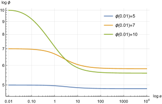
Figure 1: The numerical solution of the potentials as a function of radial distance $a$, with three different initial conditions $\phi(0.01)=5,\,7,\,10$ and $\frac{d\phi}{da}|_{a=0.01}=0$ at $a=0.01$.

With the results of potential, we can obtain the density (II) corresponds to the distribution function (1). The results is shown in Fig.2. We can see that they are almost coincidence with the famous empirical dark matter density model, i.e, NFW density profile, which has logarithmic density slope $\gamma={log\rho}/{loga}$ about $-1$ close to the center and $-3$ in the outer region of the halo, see also the $\gamma$ as a function of radial distances in Fig.3. The initial conditions will affect the logarithmic density slope near the center region, the smaller the initial potential, the more similar to the NFW model. It is remarkable that we can obtain the NFW-like density profile from a phase space distribution function.

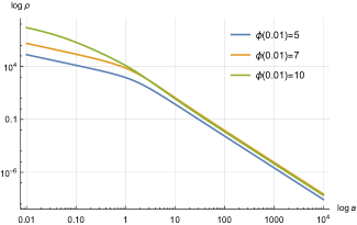
Figure 2: The numerical result of dark matter density as a function of radial distance $a$, with three different initial conditions $\phi(0.01)=5,\,7,\,10$.

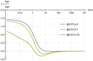
Figure 3: The logarithm slope of the dark matter density $\gamma$ as a function of radial distance $a$, with three different initial conditions $\phi(0.01)=5,\,7,\,10$.

Since our model allows one to consider anisotropic case, it is also important to investigate the anisotropy parameter $\beta$ which is defined as

$$\beta(a)\equiv 1-\frac{\sigma_{t}^{2}}{2\sigma_{r}^{2}}$$ (8)

where $\sigma_{t}$ and $\sigma_{r}$ are respectively the tangential and radial velocity dispersion. They could be compute through

$$\sigma_{r}^{2}(a) =\frac{2\pi}{\rho(a)}\int v_{r}^{2}*v_{t}f(v_{r},v_{t},a)dv_{r}dv_{t}$$ (9)

$$\sigma_{t}^{2}(a) =\frac{2\pi}{\rho(a)}\int v_{t}^{3}f(v_{r},v_{t},a)dv_{r}dv_{t}$$ (10)

We show $\beta$ as a function of $a$ in Fig.4. Despite the different initial potentials, we notice that the $\beta$s are almost the same. The initial conditions doesn’t affect the anisotropy. The $\beta$ starts from $\beta=0$, i.e., $\sigma_{t}^{2}/2=\sigma_{\theta}^{2}=\sigma_{\varphi}^{2}=\sigma_{r}^{2}$, which means that it is isotropic around the centre. As radius grows, $\beta$ increase rapidly around the scale radius $a=1$ and up to $\beta=1$ all the way through larger radial distances, which means $\sigma_{t}^{2}\ll\sigma_{r}^{2}$. In large radius, the behavior of $\beta$ is resemble the $\beta$ in Osipkov-Merritt model [42, 43]. This could be caused by the exponent of our distribution function $Q$ which is similar to the Osipkov-Merritt model.

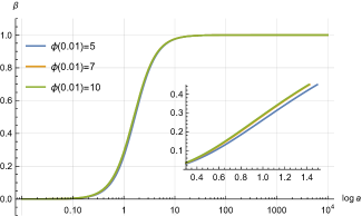
Figure 4: The anisotropy parameter $\beta$ as as a function of radial distance $a$, with three different initial conditions $\phi(0.01)=5,\,7,\,10$.

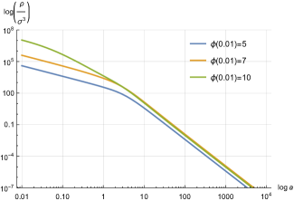
Figure 5: The pseudo phase space density as a function of radial distance $a$, with three different initial conditions $\phi(0.01)=5,\,7,\,10$.

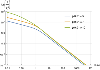
Figure 6: The quantity $\rho/\sigma_{r}^{3}$ as a function of radial distance $a$, with three different initial conditions $\phi(0.01)=5,\,7,\,10$.

We also investigate the pseudo phase space density

$$\frac{\rho}{\sigma^{3}}=\frac{\rho}{(\sigma_{t}^{2}+\sigma_{r}^{2})^{3/2}}$$ (11)

which is another important empirical laws. In Fig.5, we plot the pseudo phase space density as a function of $a$. We can see that it has pretty much the same logarithmic density slope as the density, see Fig.2. It has negative logarithmic slope as many empirical studies have shown [3, 4, 5, 44, 45, 46]. Again, the different initial potentials only cause a difference in the center region, and also quite the slope of the power law in the outer region. As comparison, we also plot the quantity $\rho/\sigma_{r}^{3}$ as as a function of radius [44]. The slopes in the outer region are the same to the pseudo phase space density, while there are an overall shift to higher values in the center region.

II.2 velocity distributions

The full velocity distribution $f(v)$ could be obtained by transformation and integrating over the distribution function (1), we have

$$f(v)\propto\frac{4\pi e^{\phi-\frac{v^{2}}{2}}\left(2\phi-v^{2}\right)\text{DawsonF}\left(\frac{1}{2}\sqrt{a^{2}v^{2}}\right)}{a\sqrt{a^{2}v^{2}}}$$ (12)

where DawsonF$(x)$ is so-called the Dawson integral. We have plotted the above full velocity distribution with different radius $a=1,\,5,\,10$ in Fig.7, by choosing the initial potential $\phi(0.01)=5$. As comparison, we also show the SHM velocity distributions which corresponds to the Maxwell-Boltzmann phase space distribution. We can see that our velocity distribution is naturally suppressed in the high velocity tails. The velocity distributions are more concentrated to low values as the radial distance become larger.

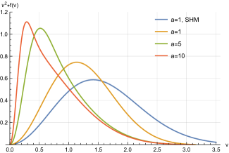
Figure 7: The normalized full velocity distribution $v^{2}f(v)$ as a function of velocity $v$, at three different radial location $a=1,\,5,\,10$, with initial potential $\phi(0.01)=5$. We also show the Maxwell-Boltzmann distribution at $a=1$, as comparison.

The above integrated velocity has some extent degeneracy over the velocity components. Therefore, it is more important to know the radial and tangential velocity distributions and verify them with simulations.

By integral over the tangent velocity component over the distribution function (1). We get the radial velocity distribution. In the same way, we can integrate over the radial velocity component over the distribution (1) and obtained the tangential velocity distribution, they are respectively given by

$$f(v_{r})\propto\frac{e^{-\frac{v_{r}^{2}-2\phi}{2\lambda^{2}}}\left(4\lambda^{2}\left(e^{\frac{\left(a^{2}+2\right)\left(v_{r}^{2}-2\phi\right)}{4\lambda^{2}}}-1\right)-v_{r}^{2}\left(a^{2}+2\right)+2\phi\left(a^{2}+2\right)\right)}{a\left(a^{2}+2\right)^{2}}$$ (13)

$$f(v_{t})\propto-\frac{e^{-\frac{\left(a^{2}+2\right)v_{t}^{2}}{4\lambda^{2}}}\left(\sqrt{2\pi}e^{\frac{\phi}{\lambda^{2}}}\left(\lambda^{2}+v_{t}^{2}-2\phi\right)\text{erf}(\frac{\sqrt{\phi-\frac{v_{t}^{2}}{2}}}{\lambda})-2\lambda e^{\frac{v_{t}^{2}}{2\lambda^{2}}}\sqrt{2\phi-v_{t}^{2}}\right)}{2a\lambda}$$ (14)

In order to fit with the real simulation data in the next section, we have kept $\lambda$ as a free parameter rather than $\lambda=1$ in the above formulas of $f(v_{r})$ and $f(v_{t})$. One could verify that the radial and tangential velocity distribution function go to zero at the local escape velocity $v_{r}=v_{t}=v_{escape}=\sqrt{2\phi}$, which means that they also have cutoff at the local escape velocity.

III comparing radial and tangential velocity distribution with simulation data

III.1 the simulation data

We use the velocity data extracted from the simulation in [47]. These numerical simulations were descried in detail previously [27, 28]. To test our model, we compare the velocity distribution function with two different scheme of simulation performed in [47].

The first is called the cold collapse simulation. This aims to simulate the violent relaxing process that occurs in the early universe when structure collapsed. They create a main halo with a number of compact and condensed substructures. All particles started with zero velocities and evolve under gravity. Once it has attained equilibrium, we divide a halo structure into radial bins (thin spherical shell) and thus we can extract the radial and tangential velocity components of the particles from selected bins. We sample the same number of particles in three radial bins whose radial and the tangential velocity data are shown in Fig.8. To make the bins data easier to read, some of the bins data have been shifted vertically. The three radial bins were chosen near the slope of $\gamma_{0}={dlog\rho}/{dlogr}=-1.6,\,-2.0,\,-2.4$.

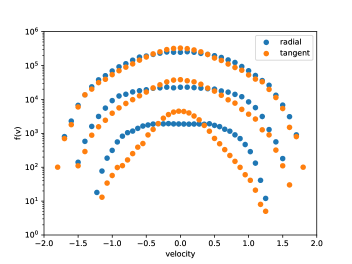
Figure 8: The three radial bins data for radial and tangential velocities in the cold collapse simulation. The three radial bins were chosen near the slope of $\gamma_{0}=-1.6,\,-2.0,\,-2.4$ (From top to bottom), and the $\gamma_{0}=-1.6,\,-2.0$ data were shifted vertically for easy reading. Each data point represents the number of particles within a velocity bin $\Delta v=0.1$.

The second set of numerically simulated data is the so-called explicit energy exchange simulation. Different types of energy exchange take place between collisionless particles, particularly through violent relaxation and dynamical friction. Therefore, the numerical set-up take into account a perturbation in which the spherical symmetry is preserved, but they permit the particles to exchange energy. Each radial bin is designed to preserve energy with instantaneous energy exchange, ensuring that the perturbation itself has no impact on the density or dispersion profiles. Subsequently, the system evolves with normal collisionless dynamics. Once again, we divide the equilibrium structure into radial bins and then extract the radial and the tangential velocity data. We plot the velocity data in Fig.9. The three radial bins were chosen near the slope of $\gamma_{0}=-1.7,\,-2.4\,-3.0$.

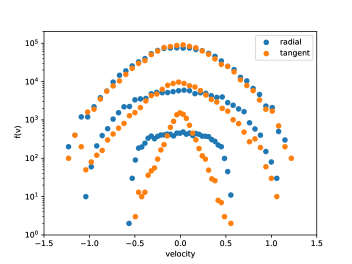
Figure 9: The three radial bins data for radial and tangential velocities in the explicit energy exchange simulation. The three radial bins were chosen near the slope of $\gamma_{0}=-1.7,\,-2.4\,-3.0$ (From top to bottom), and the $\gamma_{0}=-1.7,\,-2.4$ data were shifted vertically for easy reading. Each data point represents the number of particles within a velocity bin $\Delta v=0.07$.

III.2 fitting and parameter estimation to the velocity data

When fitting our radial and tangential velocity distribution model to the real simulation data, we adopt error-bars on these data. We assume that the horizontal (velocity) error for each data point is the width of velocity bin $\Delta v$, while the vertical (frequency) errors are the square root of the counts in each velocity bin, because we assumed that the particles in each velocity bin satisfy the Poisson distribution. We also need to add normalization factor as a free parameter to Eq.(13) and Eq.(14) respectively. So, in total, we have four parameters to fit: the normalization factor $N$, the radial distance $a$, the potential $\phi$, the parameter $\lambda$, for both radial and tangential velocity distribution functions.

From an ideal perspective, if our model is the truth, when we fit the radial and tangential data in each bin independently, there should be two constraints for the fitting parameters of the data: first, since the three radial bins data are taken from one halo structure, the value of $\lambda$ for three radial bins should be the same; second, for each radial bin, the fitting parameter ($a$, $\phi$) of radial and tangential data should also be the same. However, in practice, the radial bins have finite size and the simulation also has limiting particle numbers, so one should expect some flexibility to these two constraints.

To fit the data we employ the grid search method. Here is the procedure: first, since both radial and tangential velocity approximately converge to the same value $v_{escape}$ in each bin as velocity increases, see Fig.8 and Fig.9, we can estimate the potential of each bin from its escape velocity by $\phi\approx v_{escape}^{2}/2$. Second, we can also estimate the possible value of radial distance $a$ from the value $\gamma_{0}$ according to Fig.3. Then, we are left with the normalization factor $N$ and parameter $\lambda$ as unknown. Based on the estimated values of $a$ and $\phi$, we apply the grid search to $N$ and $\lambda$, and then exam the residuals. We take the fitting residuals as feedback again to adjust the initial estimated values of $a$ and $\phi$, and repeat the above process, until we found the approximate values for these four parameters that could minimize the residuals. In a word, what we did is trying to respect the two constraints at first, unless the data tell us that we have to modified that, and to see if our model could give an acceptable results or not. So, we intend to keep same $a$, $\phi$ and $\lambda$ values for both radial and tangential fitting in each bin during the grid search process, and modify them as necessary. As we will show, this method provide us with very good results and our velocity distribution function perform very well with these constraints within acceptable error range characterized only by radial distance $a$.

We have shown the fitting results to the three radial bins of collapse simulation in Fig.10. From top to bottom are respectively the $\gamma_{0}=-1.6,\,-2.0,\,-2.4$ bins data and fits. In each plot, we show both the radial and tangential velocity data with error-bars mentioned above. We also plot the fitting band (colored in shallow blue for radial fit, colored in shallow red for tangent fit). The band is only characterized by the radial distance $a$ while keep other parameters fixed. The fitting parameters for each bin are shown in Table.1. For $\gamma_{0}=-1.6$, the color bands are $a=1.3\pm 0.2$ for both radial and tangential fits. For $\gamma_{0}=-2.0$, the color bands are $a=2.3\pm 0.3$. For $\gamma_{0}=-2.4$, the color bands are $a=4.0\pm 0.5$. The lines represent the centre value of the color band (solid blue for radial fits, solid red for tangent fits). The reason for us to use the band is because we extract the data from radial bins and it have a finite size, so we allow the radial distance $a$ varied with an acceptable region. We also plot the residuals of the solid lines to the data (blue dots for radial fits, red dots for tangential fits).

	$\gamma_{0}=-1.5$		$\gamma_{0}=-2.0$		$\gamma_{0}=-3.0$
	rad	tan	rad	tan	rad	tan
$N$	1100	240	8800	1700	55000	7800
$a$	1.3		2.3		4.0
$\phi$	1.4		1.2		0.82
$\lambda$	0.9		1.1		1.1

Table 1: The best estimate parameter values from the radial (ran) and tangential (tan) data of three bins in the collapse simulation.

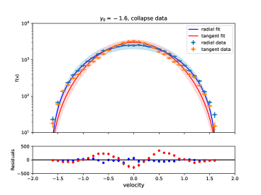
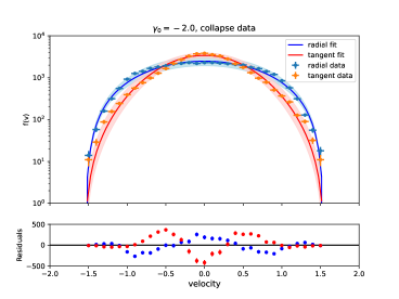
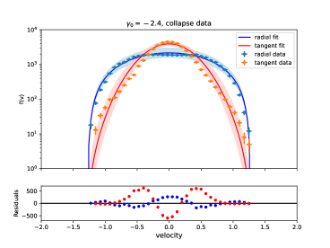
Figure 10: The radial and tangential velocity fitting results to the three radial bins in the cold collapse simulation. From top to bottom are respectively $\gamma_{0}=-1.6,\,-2.0,\,-2.4$. The radial data with errors, radial band, the center of the band as well as the residuals are are colored blue or shallow blue, while the tangential results are colored red or shallow red.

We can see from Fig.10. The smaller $\gamma_{0}$, the higher similarity of radial and tangential velocity distributions. Our model has a very good fit to all three bins velocity data, despite the residuals remained. As expected, the radial and tangential velocity converge to each other for higher velocities, while they deviate from each other at lower velocities. The radial fits are much better compare to tangential fits. The residuals grows as $\gamma_{0}$ increase, and the distribution of residuals oscillate.

In addition, from the fitting parameters in Table.1, we can see our model satisfy the two constraint in a acceptable region. If we compare the logarithm slope or $\gamma=dlog\rho/dloga$ corresponding to the fitting $a$, see Fig.3, the resulting $\gamma$ is also very close to the truth value $\gamma_{0}$ in each bin. All the results prove that our model are very promising.

	$\gamma_{0}=-1.7$		$\gamma_{0}=-2.4$		$\gamma_{0}=-3.0$
	rad	tan	rad	tan	rad	tan
$N$	60	8.8	2500	350	400000	24000
$a$	0.9		2.0		7.0
$\phi$	0.75		0.53		0.17
$\lambda$	0.48		0.65		0.69

Table 2: The best estimate parameter values from the radial (ran) and tangential (tan) data of three bins in the explicit energy exchange simulation.

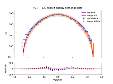
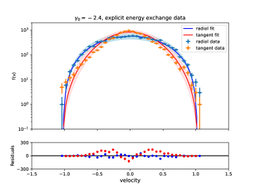
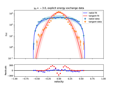
Figure 11: The radial and tangential velocity fitting results to the three radial bins in the explicit energy exchange simulation. From top to bottom are respectively $\gamma_{0}=-1.7,\,-2.4\,-3.0$. The radial data with errors, radial band, the center of the band as well as the residuals are are colored blue or shallow blue, while the tangential results are colored red or shallow red.

We have also shown the fitting results to the three radial bins of explicit energy exchange simulation in Fig.11. From top to bottom are respectively the $\gamma_{0}=-1.7,\,-2.4,\,-3.0$ bins data and fits. In each plot, we again show both the radial and tangential velocity data with errors. We also plot the fitting band. The fitting parameters for each bin are shown in Table.2. For $\gamma_{0}=-1.7$, the color bands are $a=0.9\pm 0.2$ for both radial and tangential fits. For $\gamma_{0}=-2.4$, the color bands are $a=2.0\pm 0.3$. For $\gamma_{0}=-3.0$, the color bands are $a=7.0\pm 1$. The solid lines represent the centre value of the color band. We also plot the residuals of the solid lines to the data (blue dots for radial fits, red dots for tangential fits).

We can also see from Fig.11, that for smaller $\gamma_{0}$, the higher similarity of radial and tangential velocity distributions. The pattern is repeated. Our model again has a very good fit to all three bins. The radial fits in the explicit energy exchange case is also much better than the cold collapse case. The radial fits are again much better than the tangential fits. The residuals grows as $\gamma_{0}$ increase as well, and the distribution of radial fits are quite random which means a nice fit, while the tangential residuals still oscillate.

Although there are slight differences, the similarity of the data and fits in both cold collapse and explicit energy exchange simulation reveal an universal dark matter velocity distributions. The basic trends and structures of dark matter velocity distributions were captured by our model. The data has supported our model and suggests that the model could be relevant to describe the distribution of dark matter particles.

IV conclusion and discussion

In this paper, we have suggested and analysed a model of spherically symmetric anisotropy dark matter phase space distribution function as presented in Eq. (1). We first introduced our distribution function and demonstrated their predictions on integrated quantities, which are typically analysed in numerical simulations, namely the density profile (II), the anistropy (8) and phase space density (11). In addition, we also give the full velocity (7), the radial and tangential velocity distributions in analytical forms (13) (14). In order to test the usefulness of our velocity distributions, we have respectively compared with radial and tangential velocity data which were extracted from different radial bins of equilibrium dark matter halos. We verify our results in two different simulation schemes, the cold collapse and explicit energy exchange which effectively cover a wide range of possible equilibrium processes. The fits perform quite well and the results are very promising. There are excellent agreements on estimating all the relevant parameters of the radial and tangential velocity data.

Despite the advantages of providing good fits to the velocity distributions, there are also some potentially important limitations to our model that we wish to address. First, there is a factor $r_{0}/r$ in front of the distribution function in Eq.(1), which means that the full form is not only a function of the integrals of motion. Thus this distribution function doesn’t respect to the Jeans theorem. However, this limitation doesn’t affect the results of this work since we have only suggested a phenomenological or effective model rather than a theory. Second, when comparing with the data, we can see that there exist residuals that oscillate, especially for the tangential data which seem to be the superposition of two Maxwell-Boltzmann distributions with one on the top of the other. This could revel that our model is missing some additional feature of dark matter halos.

References

- [1] M. Vogelsberger, F. Marinacci, P. Torrey and E. Puchwein, Nature Rev. Phys. 2, 42 (2020).
- [2] J. F. Navarro, C. S. Frenk, S. D. M. White, ApJ, 462, 563, (1996).
- [3] S. Cole and C. Lacey, MRNAS, 281, 716 (1996).
- [4] R. G. Carlberg, ApJ, 485, L13 (1997).
- [5] R. Wojtak, E. Lokas, S. Gottlöber, G. Mamon, MNRAS, 361, L1 (2005).
- [6] J. E. Taylor and J. F. Navarro, ApJ, 563, 483 (2001).
- [7] S. H. Hansen, B. Moore, M. Zemp and J. Stadel, JCAP, 01, 014 (2006).
- [8] J. F. Navarro et al., MNRAS, 402, 21 (2010)
- [9] B. Moore, F. Governato, T. Quinn, J. Stadel, G. Lake, ApJ, 499, 5 (1998).
- [10] J. Diemand, B. Moore, J. Stadel, MNRAS, 353, 624 (2004).
- [11] Y. P. Jing, ApJ, 535, 30 (2000).
- [12] Dan Coe, arXiv:1005.0411
- [13] C. O. Wright and T. G. Brainerd, ApJ, 534 34 (2000).
- [14] H. S. Dúmet-Montoya, G. B. Caminha, and M. Makler, A&A 560, A86 (2013).
- [15] H. Haghi, A. Khodadadi, A. Ghari, A. H. Zonoozi and P. Kroupa, MNRAS 477, 4187 (2018).
- [16] M. G. Aartsen et al. [IceCube], Eur. Phys. J. C 77, 627 (2017).
- [17] P. He, D. B. Kang, MNRAS, 406, 2678 (2010)
- [18] J. Sánchez Almeida, Universe 8, 214 (2022).
- [19] M. Vogelsberger et al., MNRAS, 395, 797 (2009).
- [20] M. Kuhlen et al., JCAP, 1002, 030 (2010).
- [21] F. S. Ling, E. Nezri, E. Athanassoula and R. Teyssier, JCAP, 1002, 012 (2010).
- [22] M. Fairbairn and T. Schwetz, JCAP, 0901, 037 (2009).
- [23] A. S. Eddington, MNRAS, 76, 572 (1916).
- [24] T. Lacroix, M. Stref and J. Lavalle, JCAP 09, 040 (2018).
- [25] S. H. Hansen, D. Egli, L. Hollenstein and C. Salzmann, New Astron. 10, 379 (2005).
- [26] J. Hjorth, L. L. R. Williams, APJ, 722, 851 (2010).
- [27] S. H. Hansen, M. Sparre, APJ, 75 100 (2012).
- [28] A. Eilersen A, S. H. Hansen, X. Zhang, MNRAS, 467, 2061 (2017).
- [29] L. Beraldo e Silva, G. A. Mamon, M. Duarte, R. Wojtak, S. Peirani and G. Boué, MNRAS, 452, 944 (2015).
- [30] I. R. King, Astron. J. 71, 64 (1966).
- [31] M. Lisanti, L. E. Strigari, J. G. Wacker and R. H. Wechsler, Phys. Rev. D 83, 023519 (2011).
- [32] Y. Y. Mao, L. E. Strigari, R. H. Wechsler, H. Y. Wu and O. Hahn, Astrophys. J. 764, 35 (2013).
- [33] T. M. Callingham, M. Cautun, A. J. Deason, C. S. Frenk, R. J. J. Grand, F. Marinacci, R. Pakmor, MNRAS, 495, 12 (2020).
- [34] N. Bozorgnia et al., JCAP 05, 024 (2016).
- [35] M. Fairbairn and T. Schwetz, JCAP 01, 037 (2009).
- [36] P. Bhattacharjee, S. Chaudhury, S. Kundu and S. Majumdar, Phys. Rev. D 87, 083525 (2013).
- [37] S. Mandal, S. Majumdar, V. Rentala and R. Basu Thakur, Phys. Rev. D 100, no.2, 023002 (2019).
- [38] B. J. Kavanagh and A. M. Green, Phys. Rev. Lett. 111, no.3, 031302 (2013).
- [39] S. K. Lee, JCAP, 03, 047 (2014).
- [40] B. J. Kavanagh, JCAP, 07, 019 (2015).
- [41] J. Binney, S. Tremaine, Galactic Dynamics, Princeton University Press, Princeton, NJ, USA (2008).
- [42] L. Osipkov, Soviet Astronomy Letters 5, 42–44 (1979).
- [43] D. Merritt, Astron. J, 90, 1027 (1985).
- [44] W. Dehnen and D. McLaughlin, MNRAS, 363, 1057 (2005).
- [45] C. G. Austin et al., Astrophys. J. 634, 756 (2005).
- [46] K. B. Schmidt, S. H. Hansen and A. V. Maccio’, Astrophys. J. Lett. 689, L33 (2008).
- [47] M. Sparre and S. H. Hansen, JCAP, 10, 049 (2012)