Relativistic effects cannot explain galactic dynamics

Abstract

It has been suggested in recent literature that non-linear and/or gravitomagnetic general relativistic effects can play a leading role in galactic dynamics, partially or totally replacing dark matter. Using the 1+3 “quasi-Maxwell” formalism, we show, on general grounds, such hypothesis to be impossible.

I Introduction

In a recent number of works, based both on linearized theory [1, 2] and exact models [3, 4, 5, 6, 7], it has been asserted that general relativistic effects (namely, gravitomagnetic ones) can have a significant impact [7, 1, 2, 5], or even totally account for the galactic flat rotation curves [6, 3, 4]. In the framework of a weak field slow motion approximation, this has been shown to be impossible, and such claims addressed, in Refs. [8, 9, 10]. It has however been argued [3, 4, 5, 7] that it is still possible in the exact theory, due to non-linear effects not captured in linearized theory (and not manifest “locally” [3, 4, 5]). In support of these claims, the Balasin-Grumiller (BG) model [5, 6, 7], or variants of it [3, 4, 7], have been used. Such model has been recently debunked in our Ref. [11], where it was shown to actually consist of a static dust, held in place by unphysical singularities along the symmetry axis, and that what actually rotates in the model are the ill chosen reference observers. In the present paper we address the general problem: assuming only stationarity of the solution, we show that (i) gravitomagnetism cannot be a relevant driving force of galactic dynamics; (ii) non-linear general relativistic effects cannot account for any amount of the needed dark matter.

Notation and conventions.— Greek letters $\alpha$, $\beta$, $\gamma$, … denote 4D spacetime indices, running 0-3; Roman letters $i,j,k,...$ are spatial indices, running 1-3; $\epsilon_{\alpha\beta\gamma\delta}\equiv\sqrt{-g}[\alpha\beta\gamma\delta]$ is the 4-D Levi-Civita tensor, with the orientation $[1230]=1$; $\epsilon_{ijk}\equiv\sqrt{h}[ijk]$ is the Levi-Civita tensor in a 3-D Riemannian manifold of metric $h_{ij}$.

II Equations of motion for massive particles and light in a stationary field

The line element $ds^{2}=g_{\alpha\beta}dx^{\alpha}dx^{\beta}$ of a stationary spacetime can generically be written as

$$ds^{2}=-e^{2\Phi}(dt-\mathcal{A}_{i}dx^{i})^{2}+h_{ij}dx^{i}dx^{j}\ ,$$ (1)

where $e^{2\Phi}=-g_{00}$, $\Phi\equiv\Phi(x^{j})$, $\mathcal{A}_{i}\equiv\mathcal{A}_{i}(x^{j})=-g_{0i}/g_{00}$, and $h_{ij}(x^{k})=g_{ij}+e^{2\Phi}\mathcal{A}_{i}\mathcal{A}_{j}$. Observers of 4-velocity $u^{\alpha}=e^{-\Phi}\partial_{t}^{\alpha}\equiv e^{-\Phi}\delta_{0}^{\alpha}$, whose worldlines are tangent to the timelike Killing vector field $\partial_{t}$, are at rest in the coordinate system of (1) (“static” observers). The quotient of the spacetime by their worldlines yields a 3-D Riemannian manifold $\Sigma$ with metric $h_{ij}$ (called the “spatial metric”), which measures the spatial distances between neighboring rest observers [12]. It is identified in spacetime with the space projector with respect to $u^{\alpha}$, $h_{\alpha\beta}\equiv g_{\alpha\beta}+u_{\alpha}u_{\beta}$.

Let $x^{\alpha}(\lambda)$ be the geodesic worldline of a test particle (that can have zero mass) and $\lambda$ an affine parameter along it. The space components of the geodesic equation $d^{2}x^{\alpha}/d\lambda^{2}=-\Gamma_{\mu\nu}^{\alpha}(dx^{\mu}/d\lambda)(dx^{\nu}/d\lambda)$ can be written as

$$\frac{d^{2}x^{i}}{d\lambda^{2}}+\Gamma(h)_{jk}^{i}\frac{dx^{j}}{d\lambda}\frac{dx^{k}}{d\lambda}=\nu\left[\nu\vec{G}+\frac{d\vec{x}}{d\lambda}\times\vec{H}\right]$$ (2)

where $\nu\equiv-u_{\alpha}dx^{\alpha}/d\lambda$,

$$\Gamma(h)_{jk}^{i}\equiv\frac{1}{2}h^{il}\left(h_{lj,k}+h_{lk,j}-h_{jk,l}\right)$$ (3)

are the Christoffel symbols of the space metric $h_{ij}$, and

$$G_{i}=-\Phi_{,i}\ ;\qquad\ H^{i}=e^{\Phi}\epsilon^{ijk}\mathcal{A}_{k,j}\quad(\epsilon_{ijk}\equiv\sqrt{h}[ijk])$$ (4)

are fields living on the space manifold $\Sigma$, dubbed, respectively, “gravitoelectric” and “gravitomagnetic” fields, for playing in Eq. (2) roles analogous to the electric and magnetic fields in the Lorentz force equation. For a 3-vector $\vec{X}$ on $\Sigma$ one can define the 3-D covariant derivative with respect to $h_{ij}$

$$\frac{\tilde{D}X^{i}}{d\lambda}\equiv\frac{dX^{i}}{d\lambda}+\Gamma(h)_{jk}^{i}X^{j}\frac{dx^{k}}{d\lambda}\ .$$ (5)

For time-like worldlines, one can set $\lambda=\tau$, so $dx^{\alpha}/d\tau\equiv U^{\alpha}$ is the 4-velocity, $\nu=-u_{\alpha}U^{\alpha}\equiv\gamma$ becomes the Lorentz factor between $U^{\alpha}$ and $u^{\alpha}$, and Eq. (2) can therefore be written as [12, 13, 14, 15, 16, 17] (cf. also [18, 19]),

$$\frac{\tilde{D}\vec{U}}{d\tau}=\gamma\left[\gamma\vec{G}+\vec{U}\times\vec{H}\right]\ ,$$ (6)

where $\vec{U}$ is the 3-vector of components $(\vec{U})^{i}=U^{i}$, tangent to the spatial curve $x^{i}(\tau)$ obtained by projecting the geodesic onto $\Sigma$. Equation (6) describes the acceleration of such 3-D projected curve [since the left-hand member of (2) is the standard 3-D covariant acceleration]. Its physical interpretation is that, from the point of view of the static observers, the spatial trajectory of the test particle will appear accelerated, as if acted upon by fictitious forces (inertial forces), arising from the fact that the reference frame is not inertial. In fact, $\vec{G}$ and $\vec{H}$ are identified in spacetime, respectively, with minus the acceleration and twice the vorticity of the static observers:

$$G^{\alpha}=-\nabla_{\mathbf{u}}u^{\alpha}\equiv-u_{\ ;\beta}^{\alpha}u^{\beta}\;;\qquad H^{\alpha}=2\omega^{\alpha}=\epsilon^{\alpha\beta\gamma\delta}u_{\gamma;\beta}u_{\delta}\;.$$ (7)

In the case of light rays (null geodesics), of tangent $k^{\alpha}=dx^{\alpha}/d\lambda$, Eqs. (2) and (5) analogously yield

$$\frac{\tilde{D}\vec{k}}{d\lambda}=\nu\left[\nu\vec{G}+\vec{k}\times\vec{H}\right]\ ;\qquad\nu\equiv-k^{\alpha}u_{\alpha}\ .$$ (8)

An equivalent formulation in terms of the photon’s null 4-momentum is given in [19], Eqs. (10.2)-(10.3), and a Lagrangian formulation in [20]. The null vector $k^{\alpha}$ decomposes, in terms of its projections parallel and orthogonal to $u^{\alpha}$, as [21]

$$k^{\alpha}=\nu(u^{\alpha}+v^{\alpha})$$ (9)

where $v^{\alpha}$ is a unit vector orthogonal to $u^{\alpha}$, yielding the photon’s spatial velocity relative to $u^{\alpha}$. Therefore, $\vec{k}=\nu\vec{v}$, and one can re-write (8) as

$$\frac{\tilde{D}\vec{k}}{d\lambda}=\nu^{2}\left[\vec{G}+\vec{v}\times\vec{H}\right]\ .$$ (10)

Equations (8)-(10) tell us that, just like massive particles, light rays in a stationary spacetime behave analogously to charged particles under the action of an electric and magnetic fields [20]. A difference, however, is that the second term in the left-hand member of (2), which reads here $\Gamma(h)_{jm}^{i}k^{j}k^{m}$, is typically of the same order magnitude as the first term in (8) [contrary to the case of $\Gamma(h)_{jm}^{i}U^{j}U^{m}=O(v^{2})$ for slowly moving massive particles].

The fields $\vec{G}$ and $\vec{H}$ obey [15]

$$\tilde{\nabla}\cdot\vec{G}=-4\pi(2\rho+T_{\ \alpha}^{\alpha})+{\vec{G}}^{2}+\frac{1}{2}{\vec{H}}^{2}\ ;\qquad\tilde{\nabla}\times\vec{G}=\ 0\ ;$$ (11)

$$\tilde{\nabla}\cdot\vec{H}=-\vec{G}\cdot\vec{H}\;;\qquad\tilde{\nabla}\times\vec{H}=-16\pi\vec{J}+2\vec{G}\times\vec{H}\ ,$$ (12)

where $\rho\equiv T^{\alpha\beta}u_{\alpha}u_{\beta}$ and $J^{\alpha}\equiv-T^{\alpha\beta}u_{\beta}$ are, respectively, the mass-energy density and current 4-vector as measured by the static observers of 4-velocity $u^{\alpha}=e^{-\Phi}\delta_{0}^{\alpha}$. Here $\tilde{\nabla}$ denotes covariant differentiation with respect to the spatial metric $h_{ij}$, with Christoffel symbols (3). The equations for $\tilde{\nabla}\cdot\vec{G}$ and $\tilde{\nabla}\times\vec{H}$ are, respectively, the time-time and time-space projections, with respect to $u^{\alpha}$, of the Einstein field equations $R_{\alpha\beta}=8\pi(T_{\alpha\beta}^{\ }-\frac{1}{2}g_{\alpha\beta}^{\ }T_{\ \gamma}^{\gamma})$; the equations for $\tilde{\nabla}\cdot\vec{H}$ and $\tilde{\nabla}\times\vec{G}$ follow from (4).

Time-like circular geodesics

In an axistationary spacetime with with reflection symmetry about the equatorial plane [22], $g_{0i}dx^{i}=g_{0\phi}d\phi$, and the angular velocity $\Omega_{{\rm geo}}\equiv d\phi/dt=U^{\phi}/U^{0}$ of circular equatorial geodesics is obtained from the Euler-Lagrange equations for the Lagrangian $\mathcal{L}=g_{\mu\nu}U^{\mu}U^{\nu}/2$, whose $r$-component $dU_{r}/d\tau=g_{\mu\nu,r}U^{\mu}U^{\nu}/2$ yields, for $U^{\alpha}=U^{0}(\delta_{0}^{\alpha}+\Omega_{{\rm geo}}\delta_{\phi}^{\alpha})$,

$$\Omega_{{\rm geo}\pm} =\frac{-g_{0\phi,r}\pm\sqrt{g_{0\phi,r}^{2}-2g_{\phi\phi,r}e^{2{\rm\Phi}}G_{r}}}{g_{\phi\phi,r}}\ .$$ (13)

The relative velocity $v^{\alpha}$ between two observers of 4-velocities $U^{\alpha}$ and $u^{\alpha}$ is defined as

$$U^{\alpha}=\gamma(u^{\alpha}+v^{\alpha})\ ;\qquad\gamma\equiv-u^{\alpha}U_{\alpha}=\frac{1}{\sqrt{1-v^{\alpha}v_{\alpha}}}\ .$$ (14)

Moreover, in the equatorial plane, given an arbitrary radial coordinate $r$, through the coordinate transformation $r_{{\rm w}}(r)=e^{\Phi(r)}\sqrt{h_{\phi\phi}(r)}$, the metric can be written in the form (1) with $h_{\phi\phi}=e^{-2\Phi}r_{{\rm w}}^{2}$. This is the case of the Weyl canonical coordinates (cf. e.g. Eq. (19.21) of [23]); it is also the case (to the accuracy at hand) of the radial coordinate $r=\sqrt{x^{2}+y^{2}}$ associated to the post-Newtonian (PN) coordinate system in Eq. (18) below. It follows from (14) that the magnitude $\|v_{{\rm geo\pm}}^{\alpha}\|=(1-\gamma_{{\rm geo\pm}}^{-2})^{1/2}$ of the velocity of the circular geodesics relative to the static observers $u^{\alpha}=e^{-\Phi}\delta_{0}^{\alpha}$ reads, in such coordinates,

$$\|v_{{\rm geo\pm}}^{\alpha}\|=\frac{2r_{{\rm w}}|G_{r_{{\rm w}}}|}{|\sqrt{-g(H^{z})^{2}-4r_{{\rm w}}G_{r_{{\rm w}}}(1+r_{{\rm w}}G_{r_{{\rm w}}})}\pm\sqrt{-g}H^{z}|}$$ (15)

where we have noted, from (4), that $\mathcal{A}_{\phi,r}=e^{-\Phi}\epsilon_{r\phi i}H^{i}=e^{-2\Phi}\sqrt{-g}H^{z}$.

II.1 Gravitomagnetism cannot be the culprit — gravitational lensing

One of the most compelling indications of the existence of dark matter halos around galaxies is the observed galactic gravitational lensing, which cannot be accounted for based only on the visible baryonic matter. It is well known that, when the emitting object (source), the foreground galaxy (lens), and the observer are nearly aligned (see Fig 1), roughly circular rings (Einstein rings [24, 25]) are formed, as in the case of the system B1938+666 [26, 27] (the first detected complete Einstein ring), or the “Cosmic Horseshoe” J1148+1930 [28, 29, 30, 31, 32]. The majority of the mass causing such lensing effect is estimated to consist of dark matter [29, 30, 31, 32, 27], and is consistent with the halos’ shape being roughly spherical or moderately deformed (namely prolate [31], as seems to be more common [33]). Anomalies in such rings have actually been recently proposed [34] as a mean of determining the nature of dark matter, namely distinguishing between weakly interacting massive particles and axions.

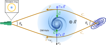
Figure 1: Gravitational lensing by galactic dark matter halos. When the observer, foreground, and emitting galaxies are aligned, an Einstein ring forms. Nearly perfect Einstein rings have been detected, such as in the system B1938+666, or the “Cosmic Horseshoe” J1148+1930. The majority of the lensing effect is estimated to come from dark matter. The gravitomagnetic field cannot mimic such effects, since the inertial force $\vec{v}\times\vec{H}$ does not contribute to make light rays converge in such setting; e.g., in the equatorial plane, it deflects photons on both sides of the body in the same direction. (The effect being anyway negligible for any realistic galactic model).

These effects could not take place if it was the gravitomagnetic field $\vec{H}$ the main driver of galactic dynamics. For a rotating body, under the assumptions of stationarity and reflection symmetry about the equatorial plane, $\vec{H}$ is axisymmetric, orthogonal to the equatorial plane, and pointing in the same direction along the whole plane. It follows from Eq. (10) that the gravitomagnetic “force” $\vec{v}\times\vec{H}$ on light rays passing through opposite sides of the body points in the same direction, thus not contributing to produce convergence of light rays along the line of sight of observers aligned with the foreground galaxy (setting illustrated in Fig. 1). This can be seen also using the Gauss-Bonnet theorem [35, 36, 37, 38, 39, 40, 41]: the light ray trajectories $C_{\pm}$ illustrated in Fig. 1 are the projections of the photon’s null geodesics $C_{\pm}^{(4)}$ onto the space manifold $\Sigma$, $\pi_{\Sigma}C_{\pm}^{(4)}=C_{\pm}$. Let $\mathcal{S}$ be an oriented 2-surface on $\Sigma$ bounded by $C_{\pm}$: $\partial\mathcal{S}=C_{+}\cup(-C_{-})$, where $-C_{-}$ is the curve with the opposite orientation of $C_{-}$. Then

$$\theta_{{\rm R}}=\iint_{\mathcal{S}}Kd\mathcal{S}+\int_{C_{+}}\kappa_{{\rm g}}d\lambda-\int_{C_{-}}\kappa_{{\rm g}}d\lambda-\theta_{{\rm S}}-2\pi[\chi(\mathcal{S})-1]\ ,$$ (16)

where $K$ is the Gaussian curvature of $\mathcal{S}$ and $\chi(\mathcal{S})$ its Euler characteristic (if simply connected, namely in the absence of singularities, $\chi(\mathcal{S})=1$), and $\kappa_{{\rm g}}$ is the geodesic curvature [42, 43, 35] of a curve $C$ of tangent vector $\dot{C}(\lambda)$. Considering a positively oriented orthonormal frame $\{e_{\hat{1}},e_{\hat{2}}\}$ on $\mathcal{S}$ along $C$ such that $e_{\hat{1}}=\dot{C}/\|\dot{C}\|$ (see Fig. 1), the geodesic curvature of $C$ is given by [42]

$$\kappa_{{\rm g}}=\frac{1}{\|\dot{C}\|}\langle\tilde{\nabla}_{\dot{C}}e_{\hat{1}},e_{\hat{2}}\rangle=\frac{\langle\tilde{\nabla}_{\dot{C}}\dot{C},e_{\hat{2}}\rangle}{\|\dot{C}\|^{2}}\ ,$$

where $\tilde{\nabla}$ is the Levi-Civita covariant derivative of $(\Sigma,h)$, with Christoffel symbols (3), as defined above. For light rays, $\dot{C}=\vec{k}$, $\|\dot{C}\|^{2}=h_{\alpha\beta}k^{\alpha}k^{\beta}=\nu^{2}$ [cf. Eq. (9)], and $\hat{e}_{\hat{1}}=\vec{v}$. Recalling that the left-hand member of (2) is the 3-D covariant acceleration $\tilde{\nabla}_{\dot{C}}\dot{C}$, by Eq. (10) we have $\tilde{\nabla}_{\dot{C}}\dot{C}=\nu^{2}[\vec{G}+\vec{v}\times\vec{H}]$; hence

$$\kappa_{{\rm g}}=\langle\vec{G},e_{\hat{2}}\rangle+\langle\vec{v}\times\vec{H},e_{\hat{2}}\rangle\equiv G^{\hat{2}}+(\vec{v}\times\vec{H})^{\hat{2}}\ .$$

For the setting in Fig. 1, in the equatorial plane, $(\vec{v}_{\pm}\times\vec{H})^{\hat{2}}=-\|\vec{H}\|$; hence, the gravitomagnetic contributions to the convergence angle $\theta_{{\rm R}}$ in Eq. (16) have opposite signs. In particular, for the case where the rays are approximately symmetric, as required for a nearly perfect Einstein ring, we have, due to the reflection symmetry about the $y=0$ plane, $\int_{C_{+}}\|\vec{H}\|d\lambda\approx\int_{C_{-}}\|\vec{H}\|d\lambda$ and $\int_{C_{+}}G^{\hat{2}}d\lambda\approx-\int_{C_{-}}G^{\hat{2}}d\lambda$; therefore

$$\int_{C_{+}}\kappa_{{\rm g}}d\lambda-\int_{C_{-}}\kappa_{{\rm g}}d\lambda\approx 2\int_{C_{+}}G^{\hat{2}}d\lambda\ ,$$

so the gravitomagnetic force does not contribute to $\theta_{{\rm R}}$ in Eq. (16). Indeed, the effect of the gravitomagnetic force would be to cause the light rays that reach an observer aligned with the source and foreground galaxy to arrive at different angles from each side, as exemplified in Appendix A for the case of a Kerr black hole (completely distorting the ring if such force was comparable, or even several times larger than the gravitoelectric force, as would be required for it to explain the galactic rotation curves). Moreover, in the far field regime, the gravitomagnetic field of a galaxy (as for any spinning body) is dipole-like, as illustrated in Fig. 2; hence, light rays with impact parameter $\vec{b}$ orthogonal to the equatorial plane, are deflected in a direction parallel to that plane (thus orthogonal to $\vec{b}$), which again produces no convergence, cf. Secs. III.1.3 and Appendix A.

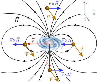
Figure 2: Gravitomagnetic field $\vec{H}$ produced by a galactic disk. At large distances, it is dipole-like, deflecting photons with impact parameter $\vec{b}$ orthogonal to the equatorial plane in a direction opposite to those for which $\vec{b}$ lies in the equatorial plane (in both cases, photons through opposite sides of the body being deflected in the same direction); this produces no convergence of light rays along the line of sight of observers aligned with the foreground galaxy.

II.2 Non-linear GR effects work against attraction

Since the gravitomagnetic field $\vec{H}$ cannot be relevant, the motion of massive bodies is ruled by the first term of Eq. (6). From (15), we have, for the velocity of the circular equatorial geodesics in an axistationary spacetime, when $\vec{H}$ is neglected,

$$\|v_{{\rm geo\pm}}^{\alpha}\|\approx\sqrt{\frac{-G_{r_{{\rm w}}}}{G_{r_{{\rm w}}}+1/r_{{\rm w}}}}$$ (17)

which, likewise, is ruled by $G^{\alpha}$ [observe that, for the PN metric in Eq. (18) below, $r_{{\rm w}}=\sqrt{x^{2}+y^{2}}$, and so linearizing Eq. (17) yields the Newtonian rotation curve $v=\sqrt{-rG_{r}}$]. The same conclusion can be reached from the angular velocity (13), neglecting the gravitomagnetic potential $\bm{\mathcal{A}}=\mathcal{A}_{\phi}{\bf d}\phi=e^{-2\Phi}g_{\phi 0}{\bf d}\phi$, which leads to $\Omega_{{\rm geo}\pm}=e^{{\rm\Phi}}(-2G_{r}/g_{\phi\phi,r})^{1/2}$ (where one can take $g_{\phi\phi}=r^{2}$, since it is well known from experiment that the galactic space metric is very weakly curved).

Thus it remains only to clarify whether non-linear GR effects can amplify $\vec{G}$ in order to produce an attractive effect able to sustain the rotation curves. It is clear however, from the first of Eqs. (11), that the non-linear terms ${\vec{G}}^{2}$ and ${\vec{H}}^{2}/2$ act as effective negative “energy” sources for $\vec{G}$ [13], countering the attractive effect of the source term $2\rho+T_{\ \alpha}^{\alpha}$ ($=\rho$ for dust). Hence, they only aggravate the need for dark matter. This is manifest already in post-Newtonian (PN) theory, see Sec. III.1 below. It is also clear, based on PN theory, that the effect is anyway negligible in any realistic galactic model, given the weakness of the galactic gravitational potential (cf. Secs. III.1.1 and III.1.2). It is huge, however, in some galactic models proposed in the literature. Namely, in the Balasin-Grumiller dust model (Sec. III.2 below), the effect is such that it completely kills off the attractive contribution from the dust’s mass density $\rho$, yielding $\vec{G}=0$ [11].

III Relevant examples

III.1 Post-Newtonian theory

In the post-Newtonian (PN) expansion of general relativity, at first (1PN) order, the metric can be written, in geometrized units, as [44, 45, 46]

$$g_{00} =-1+2w-2w^{2}+O(6)\ ;$$

$$g_{i0} =\mathcal{A}_{i}+O(5)\ ;\qquad g_{ij}=\delta_{ij}\left(1+2w\right)+O(4)\ ,$$ (18)

where $O(n)\equiv O(\epsilon^{n})$, $\epsilon$ is a small dimensionless parameter such that $U\sim\epsilon^{2}$, $U$ is minus the Newtonian potential, and $w=U+O(4)$ consists of the sum of the Newtonian potential $U$ plus non-linear terms of order $\epsilon^{4}$. The bodies’ velocities are assumed such that $v\lesssim\epsilon$ (since, for bounded orbits, $v\sim\sqrt{U}$), and time derivatives increase the degree of smallness of a quantity by a factor $\epsilon$; for example, $\partial U/\partial t\sim Uv\sim\epsilon U$. The geodesic equation for a test particle can be written as [44]

$$\frac{d^{2}\vec{x}}{dt^{2}}=(1+v^{2}-2U)\vec{G}+\vec{v}\times\vec{H}-3\frac{\partial U}{\partial t}\vec{v}-4(\vec{G}\cdot\vec{v})\vec{v}+O(6)\$$ (19)

with

$$\vec{G}=\nabla w-\frac{\partial\vec{\mathcal{A}}}{\partial t}+O(6)\ ;\quad\vec{H}=\nabla\times\vec{\mathcal{A}}+O(5)\ .$$ (20)

In the stationary case (i.e., neglecting all time derivatives), Eq. (19) yields the post-Newtonian limit of Eq. (6), as can be seen noting that $\tilde{D}\vec{U}/d\tau=(U^{0})^{2}d^{2}\vec{x}/dt^{2}-v^{2}\vec{G}+4(\vec{G}\cdot\vec{v})\vec{v}+O(6)$ and $(U^{0})^{-2}=1-v^{2}-2U+O(4)$.

III.1.1 System of $N$ point bodies

For a system of $N$ gravitationally interacting point particles, the metric potentials read, in the harmonic gauge (e.g. [44, 47, 46, 48]),

$$w =\sum_{{\rm a}}\frac{M_{{\rm a}}}{r_{{\rm a}}}\left(1+2v_{{\rm a}}^{2}-\sum_{{\rm b\neq a}}\frac{M_{{\rm b}}}{r_{{\rm a}{\rm b}}}-\frac{1}{2}\vec{r}_{{\rm a}}\cdot\vec{a}_{{\rm a}}-\frac{(\vec{r}_{{\rm a}}\cdot\vec{v}_{{\rm a}})^{2}}{2r_{{\rm a}}^{2}}\right)$$

$$\vec{\mathcal{A}} =-4\sum_{{\rm a}}\frac{M_{{\rm a}}}{r_{{\rm a}}}\vec{v}_{{\rm a}}\ ;\qquad U=\sum_{{\rm a}}\frac{M_{{\rm a}}}{r_{{\rm a}}}\ ,$$ (21)

where $M_{{\rm a}}$ is the mass of particle “a”, $\vec{r}_{{\rm a}}\equiv\vec{x}-\vec{x}_{{\rm a}}$, $\vec{x}$ is the point of observation, $\vec{x}_{{\rm a}}$ is the instantaneous position of particle “${\rm a}$”, $\vec{v}_{{\rm a}}=\partial\vec{x}_{{\rm a}}/\partial t$ its velocity, $\vec{a}_{{\rm a}}=\partial\vec{v}_{{\rm a}}/\partial t$ its coordinate acceleration, and $\vec{r}_{{\rm a{\rm b}}}\equiv\vec{x}_{{\rm a}}-\vec{x}_{{\rm b}}$. The gravitoelectric and gravitomagnetic fields (20) read

$$\vec{G} =-\sum_{{\rm a}}\frac{M_{{\rm a}}}{r_{{\rm a}}^{3}}\vec{r}_{{\rm a}}\left[1-2\sum_{{\rm b}}\frac{M_{{\rm b}}}{r_{{\rm b}}}-\sum_{{\rm b\neq a}}\frac{M_{{\rm b}}}{r_{{\rm a}{\rm b}}}\right.$$

$$\left.+2v_{{\rm a}}^{2}-\frac{3(\vec{r}_{{\rm a}}\cdot\vec{v}_{{\rm a}})^{2}}{2r_{{\rm a}}^{2}}-\frac{1}{2}(\vec{r}_{{\rm a}}\cdot\vec{a}_{{\rm a}})\right]$$

$$+3\sum_{{\rm a}}\frac{M_{{\rm a}}}{r_{{\rm a}}^{3}}(\vec{r}_{{\rm a}}\cdot\vec{v}_{{\rm a}})\vec{v}_{{\rm a}}+\frac{7}{2}\sum_{{\rm a}}M_{{\rm a}}\frac{\vec{a}_{{\rm a}}}{r_{{\rm a}}}\ ;$$ (22)

$$\vec{H} =-4\frac{M_{{\rm a}}}{r_{{\rm a}}^{3}}\sum_{{\rm a}}\vec{v}_{{\rm a}}\times\vec{r}_{{\rm a}}\ .$$ (23)

In the case of a single body at rest, the potentials (21) reduce to $w=M/r$, $\vec{\mathcal{A}}=0$, and (18) yields the 1PN limit of the Schwarzschild metric in isotropic or harmonic coordinates (obtained, to the accuracy at hand, from the usual Schwarzschild coordinates $\{t,\varrho,\theta,\phi\}$ through the substitution $\varrho=r+M$, cf. e.g. [48] pp. 268-270). Equations (22)-(23) yield in this case $\vec{H}=0$ and

$$\vec{G}=-\frac{M}{r^{3}}\left(1-\frac{2M}{r}\right)\vec{r}\ .$$

This is smaller than the Newtonian (0PN) gravitoelectric field $\vec{G}_{{\rm N}}=-\vec{r}M/r^{3}$, showing that the non-linear contribution decreases the gravitational attraction. The angular velocity of circular geodesics, Eq. (13), is

$$\Omega_{{\rm geo\pm}}=\pm\left[\sqrt{\frac{M}{r^{3}}}-\frac{3}{2}\sqrt{\frac{M^{3}}{r^{5}}}\right]\ ,$$

which, accordingly, is slower than the Newtonian angular velocity $\Omega_{{\rm N}}=\pm M^{1/2}/r^{3/2}$.

Stars in a galaxy can be considered, to a good approximation, point masses. In the Milky Way their velocities are of the order $v_{{\rm a}}\sim 10^{-3}$, and their acceleration $a_{{\rm a}}$ of the order $v_{{\rm a}}^{2}/r\sim 10^{-6}/r$; hence, the velocity and acceleration dependent terms in (22) are smaller by a $10^{6}$ factor compared to the Newtonian term $\vec{G}_{{\rm N}}=-\sum_{{\rm a}}M_{{\rm a}}\vec{r}_{{\rm a}}/r_{{\rm a}}^{3}$. The same applies to the velocity dependent terms in (19), by Eqs. (21)-(23). The remaining relativistic corrections are the non-linear terms in the first line of Eq. (22) (which are negative, thus decreasing the magnitude of $\vec{G}$), plus the negative term $-2U\vec{G}$ in (19); all of them decrease the attraction, thus working against the sought effect for explaining the galactic rotation curves (the corrections being anyway negligible, comparing to the Newtonian terms).

III.1.2 Self gravitating disks

The gravitational field of self-gravitating stationary fluids is described, to first post-Newtonian order, by the metric (18) with $w=U$ [49, 50]. The relativistic Euler equations are integrable provided that the angular momentum per unit mass $j$ depends only on the angular velocity $\Omega$ [49]. A function $j(\Omega)$, appropriate for toroids, is given in Eq. (8) of [49]; specializing to thin hollow disks of dust (case that could represent stars in a disk galaxy), the rotation curve obtained is

$$\Omega=\Omega_{{\rm N}}-\frac{2}{1-\delta}\Omega_{{\rm N}}^{3}r^{2}-\frac{\mathcal{A}_{\phi}}{r^{2}(1-\delta)}$$ (24)

(cf. Eq. (18) of [49]), where $\Omega_{{\rm N}}$ is the Newtonian result, $\delta\in[-\infty,0]\setminus\{-1\}$ is a parameter, and $\mathcal{A}_{\phi}$, from its definition in e.g. Eqs. (8.4) of [48], is of order $\mathcal{A}_{\phi}/r^{2}\sim 10^{-3}U/r\sim 10^{-6}\Omega_{{\rm N}}$ for the Milky Way (in agreement with the conclusion in [8]), thus negligible. The non-linear contribution in the second term, again, slows down the rotation (being anyway also negligible for the Milky Way, where $\Omega_{{\rm N}}^{2}r^{2}\sim 10^{-6}$).

III.1.3 Lensing around a spinning body

The gravitational field of any isolated stationary matter distribution is described, to linear order, by the metric

$$ds^{2}=(-1+2U)dt^{2}+2\mathcal{A}_{i}dx^{i}+\delta_{ij}\left(1+2U\right)dx^{i}dx^{j}\ ,$$

which follows from linearizing (18) with $\vec{\mathcal{A}}=2\vec{r}\times\vec{S}/r^{3}$, where $\vec{S}$ is the distribution’s angular momentum (cf. e.g. Eq. (27.32) of [51]). Notice that this is a dipole-type vector potential, of dipole moment $-2\vec{S}$. The corresponding gravitomagnetic field is [cf. Eqs. (20)] $\vec{H}=2\vec{S}/r^{3}-6(\vec{S}\cdot\vec{r})\vec{r}/r^{5}$, formally identical to the magnetic field of a magnetic dipole of moment $\vec{\mu}=-2\vec{S}$, as is well known (e.g. [52]).

Consider light rays from a distant source, at impact parameter $\vec{b}$, being scattered by the distribution (see e.g. Fig. 1 of [53]). The change in the ray direction, $\Delta\vec{v}=\vec{v}_{{\rm f}}-\vec{v}_{{\rm in}}$, is given by $\Delta\vec{v}=2\int_{-\infty}^{\infty}\vec{G}dt+\Delta\vec{v}_{{\rm H}}$, where $\vec{G}=\nabla U$ and

$$\Delta\vec{v}_{H}=\frac{4}{b^{2}}\left[\frac{2}{b^{2}}(\vec{b}\cdot(\vec{v}_{{\rm in}}\times\vec{S})\vec{b}-(\vec{v}_{{\rm in}}\times\vec{S})\right]$$

is the gravitomagnetic deflection [54, 53]. Hence, for pairs of light rays at opposite impact parameters $\pm\vec{b}$ (see Fig. 2), $\Delta\vec{v}_{H}$ is the same, thus not contributing to produce convergence. For $\vec{v}_{{\rm in}}$ and $\vec{b}$ mutually orthogonal an lying in the equatorial plane (e.g. $\vec{v}_{{\rm in}}=\|\vec{v}_{{\rm in}}\|\vec{e}_{x}$, $\vec{b}=\pm\|\vec{b}\|\vec{e}_{y}$, $\vec{S}=\|\vec{S}\|\vec{e}_{z}$, as depicted in Fig. 2), the photons are deflected in the direction $\hat{v}_{{\rm in}}\times\hat{S}$ ($=-\vec{e}_{y}$, in Fig. 2) along the equatorial plane; for the same $\vec{v}_{{\rm in}}$, but now $\vec{b}$ orthogonal to the equatorial plane ($\vec{b}\parallel\pm\vec{S}$), the photons are again deflected parallel to the equatorial plane, but now in the opposite direction $-\hat{v}_{{\rm in}}\times\hat{S}$.

III.2 The Balasin-Grumiller (BG) “galactic” model

The BG solution is described by the metric [5]

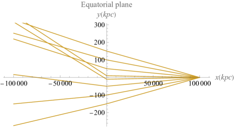
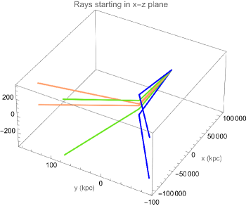
Figure 3: Gravitational light deflection (numerical results) in the Balasin-Grumiller solution for $r_{0}=1\,{\rm kpc}$, $R=100\,{\rm kpc}$, $V_{0}=220\,{\rm km/s}$, $\mu\approx 1$, and a light source at a distance $100\,{\rm Mpc}$. Left panel: in the equatorial plane, light rays through opposite sides of the body are deflected in the same direction. Right panel: light rays starting out in the $z_{O}x$ plane. Each color corresponds to a pair of rays with symmetric angles about the equator; these are made to diverge along the $z$-direction, and are moreover deflected along the positive $y$-direction if they approach the $z$-axis at $|z|<R$, and in the opposite direction at $|z|>R$. This is consistent with the presence of a pair of axial (oppositely charged) NUT rods located at $r_{0}<|z|<R$, whose gravitomagnetic field (Fig. 5 of [11]) drives the deflection. Multiple images of the source occur at some points, namely on the $y>0$ side of the equatorial plane, where light rays cross; but no Einstein rings are possible.

$$ds^{2} =-(dt-Nd\phi)^{2}+r^{2}d\phi^{2}+e^{\mu}(dr^{2}+dz^{2})\ ;$$ (25)

$$N(r,z) =\frac{V_{0}}{2}\sum_{\pm}\left[\sqrt{(z\pm r_{0})^{2}+r^{2}}-\sqrt{(z\pm R)^{2}+r^{2}}\right]$$

$$\quad+V_{0}(R-r_{0})\ ,$$ (26)

claimed to describe a galactic dust model in comoving coordinates, with $r_{0}$ the radius of the bulge region, and $R$ roughly the radius [6] of the galactic disk in the equatorial plane. It has however been recently shown in [11] to actually consist of a dust static with respect to the asymptotic inertial frame (hence totally unsuitable as a galactic model), held in place by unphysical singularities along the symmetry axis, and the claimed flat rotation curves to be but an artifact of an unsuitable choice of reference observers (the ZAMOs, which undergo circular motions with respect to inertial frames at infinity, due to the artificially large frame-dragging effects created by the singularities). It turns out to be also an archetypal example for Secs. II.1 and II.2.

Since $\vec{G}=0$ and $\vec{J}=0$ [11], Eqs. (11)-(12) yield $\tilde{\nabla}\cdot\vec{H}=0$, $\tilde{\nabla}\times\vec{H}=0$, and

$$\tilde{\nabla}\cdot\vec{G}=-4\pi\rho+\frac{1}{2}{\vec{H}}^{2}=0\ .$$ (27)

Linearization of this equation leads to the empty space equation $\rho=0$; hence, the solution has no linear or Newtonian limit, being thus a purely non-linear solution. In fact, it is an extreme example of the phenomenon discussed in Sec. II.2: the repulsive action of the non-linear contribution $\vec{H}^{2}/2$ is such that it cancels out exactly the attractive gravitational effect of the dust’s energy density (allowing the gravitoelectric field $\vec{G}$ to vanish [11]).

The equation for null geodesics, from Eqs. (2), (8), and (10), becomes here

$$\frac{d^{2}x^{i}}{d\lambda^{2}}+\Gamma(h)_{jl}^{i}k^{j}k^{l}=\nu\vec{k}\times\vec{H}=\nu^{2}\vec{v}\times\vec{H}\ .$$

If one approximates, as done in [5], $\mu\approx{\rm const}.$, the space metric $h_{ij}$ becomes flat, $\Gamma(h)_{jl}^{i}$ become the Christoffel symbols of a cylindrical coordinate system in Euclidean space, and the spacetime an example of a solution where light deflection is solely driven by the gravitomagnetic “force” $\nu^{2}\vec{v}\times\vec{H}$. The numerical results, for the parameters suggested in [5] for the Milky Way ($r_{0}=1\,{\rm kpc}$, $R=100\,{\rm kpc}$, $V_{0}=220\,{\rm km/s}$) and a light source at a distance $100\,{\rm Mpc}$ (roughly 100 times the average distance between nearby galaxies), is plotted in Fig. 3. They are consistent with the expectation for the gravitomagnetic field as plotted in Fig. 5 of [11], generated by a pair of oppositely charged NUT rods along the $z$-axis located at at $r_{0}<z<R$ and $-R<z<-r_{0}$: in the equatorial plane, where $\vec{H}|_{z=0}=|H|\partial_{z}$ points always in the same direction orthogonal to the plane, light rays passing through opposite sides of the galaxy are deflected in the same direction (the $\partial_{y}$ direction). Some light rays cross on the $y>0$ side, but not along the line of sight of an observer aligned with the source and foreground galaxy. Light rays whose direction lies, initially, along the $z_{O}x$ plane, never cross. Hence, as expected, such a model cannot produce lensing effects such as the Einstein rings observed in [26, 27].

III.3 Gravitomagnetic dipole model

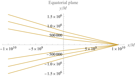
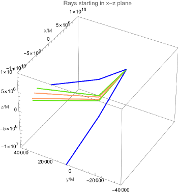
Figure 4: Gravitational light deflection (numerical results) in the gravitomagnetic dipole model, for $Q_{{\rm NUT}}=\pm M$, separation $2k=3.6\times 10^{6}M$, and a light source at a distance $r=10^{10}M$. No convergence of light rays is produced, which immediately rules out this setting as a viable galactic model. Left panel: rays in the equatorial plane are made to diverge. Right panel: light rays starting out in the $z_{O}x$ plane (each color corresponds to a pair of rays with symmetric angles about the $x$-axis). They are deflected orthogonally to that plane; along the negative $y$- direction if they approach the $z$-axis at $|z|\lesssim 10^{10}M$ (more strongly in the region between the two NUT black holes, $|z|<1.8\times 10^{6}M$), and in the opposite direction otherwise (not shown). This is consistent with the expectation from the gravitomagnetic field plotted in Fig. 5.

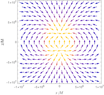
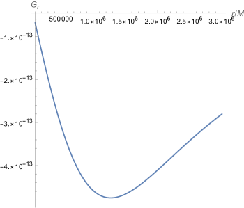
Figure 5: Left panel: $x$-$z$ plot of the gravitomagnetic field $\vec{H}$ for the gravitomagnetic dipole model with $Q_{{\rm NUT}}=\pm M$, and separation $2k=3.6\times 10^{6}M$; color represents field strength (blue=weak, yellow=strong). Right panel: radial component of the equatorial gravitoelectric field $\vec{G}$, as a function of $r$. Albeit attractive, $|G_{r}|$ does not monotonically decrease with $r$.

In [55] a galactic model based on a so called “gravitomagnetic dipole” is proposed. It consists of the solution obtained in [56, 57] from a (non-linear) superposition of two NUT solutions, interpreted as a pair of NUT “objects” of equal masses and equal in magnitude, but opposite, NUT charges. The lengthy expression for the metric is given in Eqs. (1)-(10) of [55]. It depends only on three parameters: the mass $M$ and NUT charge $\pm Q_{{\rm NUT}}$ ($\pm\nu$, in the notation of [55, 56]) of each object, and their separation $2k$. For sufficiently large $k$, the objects are interpreted as a pair of NUT black holes connected by a spinning Misner string [55]. The gravitomagnetic field (4) plotted in Fig. 5 is indeed consistent with a pair of opposite gravitomagnetic monopoles (NUT singularities). We choose the values $\nu\simeq M$ and $k=1.8\times 10^{6}M$ as proposed in Eqs. (82) and (85) of [55]. This yields, for circular equatorial geodesics, a nearly flat velocity profile with $v\approx 8\times 10^{-4}$ within the range $4\times 10^{5}<r/M<1.5\times 10^{6}$ [55]; for $M=2.6\times 10^{11}M_{\odot}$ ($M_{\odot}\equiv$ solar mass) this corresponds to $5\ {\rm kpc}<r<19\ {\rm kpc}$, approximately matching the observed flat region of the Milky Way rotation curve.

The trajectories of light rays emitted from a foreground galaxy at $r=10^{10}M$, corresponding (again, for $M=2.6\times 10^{11}M_{\odot}$) to $10^{2}{\rm Mpc}$, i.e., roughly 100 times the average distance between nearby galaxies, is plotted in Fig. 4. No convergence of light rays emitted from a foreground galaxy is produced (thus no Einstein rings, nor multiple image of the source); the rays diverge. This completely rules out this model as a viable galactic model.

Light rays starting in the equatorial plane diverge along that plane; the effect however is actually not caused by the gravitomagnetic field. It occurs as well when $Q_{{\rm NUT}}=0\Rightarrow\vec{\mathcal{A}}=\vec{H}=0$ (in which case the setting is held static by the tension of the string). In fact, the plot corresponding to $Q_{{\rm NUT}}=0$ is only slightly changed comparing to the left panel of Fig. 4, being then symmetric with respect to the $x$-axis. The effect (which, in appearance, reminds a repulsive scattering) occurs as well for massive particles (i.e., time-like worldlines). Inspection of the radial equation $d^{2}r/d\tau^{2}=-\Gamma_{\alpha\beta}^{r}U^{\alpha}U^{\beta}$ shows that it stems from the weakness of the attractive term $-\Gamma_{00}^{r}E^{2}(g^{00})^{2}=e^{-2\Phi}G^{r}E^{2}$ (see Footnote 1; here $E\equiv-U_{\alpha}\partial_{t}^{\alpha}=-U_{0}$ is the particle’s energy per unit mass), due to the unusual behavior of the gravitoelectric field $\vec{G}$, plotted in Fig. 5: although always attractive ($G_{r}<0$), its magnitude does not monotonically increase with decreasing $r$; in fact, within the region $r/M<1.5\times 10^{6}$ (which includes the flat profile range), $|\vec{G}|$ decreases approaching $r=0$, with $\lim_{r\rightarrow 0}\vec{G}=0$. This contrasts with e.g. the situation in the Schwarzschild geometry (where $|G_{r}|$ monotonically increases until the horizon, where $\lim_{r\rightarrow r_{+}}G_{r}=-\infty$), or in a Levi-Civita or Lewis-Weyl cylinders [16], and causes the centrifugal term $-\Gamma_{\phi\phi}^{r}L^{2}(g^{\phi\phi})^{2}=(1/2)g_{\phi\phi,r}L^{2}(g^{\phi\phi})^{2}/g_{rr}$ to sharply dominate the scattering (hence the apparent repulsion). Here $L\equiv U_{\alpha}\partial_{\phi}^{\alpha}=U_{\phi}$ is the test particle’s angular momentum per unit mass. The same conclusion can be reached by inspecting the effective potential $V_{{\rm eff}}(E,L,r)$ that follows from the equation $U^{\alpha}U_{\alpha}=-1\Leftrightarrow(dr/d\tau)^{2}=-2V_{{\rm eff}}$, so that $d^{2}r/d\tau^{2}=-dV_{{\rm eff}}/dr$.

Light rays starting out in the $z_{O}x$ plane are deflected orthogonally to that plane, via the action of the gravitomagnetic field.

It should moreover be noted that (as correctly noticed in [55]) the $z$-distance $2k=3.6\times 10^{6}M$ between the NUT black holes is comparable or larger than the galaxy size, which adds to the unrealistic character of the model.

IV Conclusion

We have shown that, in the face of the experimentally measured galactic rotation curves and gravitational lensing, not only general relativity cannot explain galactic dynamics based only on the visible baryonic matter, as taking into account non-linear corrections only aggravates the problem. In the process we wrote the equations for light propagation in the quasi-Maxwell formalism, and by gravitational lensing ruled out any galactic model (linear or non-linear) based on gravitomagnetism, as well as the recent “dipole” models (gravitomagnetic or not, linear or not).

Acknowledgments

We thank A. Pollo, E. Malec, P. Mach, and D. Grumiller for correspondence and very useful discussions. L.F.C. and J.N. were supported by FCT/Portugal through projects UIDB/MAT/04459/2020 and UIDP/MAT/04459/2020.

Appendix A Lensing in the Schwarzschild and Kerr spacetimes

For comparison with the models in Secs. III.2 and III.3, in order to evince their unphysical character, we present in Fig. 6 the corresponding plots of the lensing effects produced by a Schwarzschild black hole (displaying some essential features common to other compact and spherically symmetric sources) and, to evince the role of the gravitomagnetic field, of a fast spinning Kerr black hole. In the Schwarzschild case, the deflection is the same for rays starting at equal (in magnitude) angles relative to the axis connecting the source and the black hole ($x$-axis); this leads to perfectly circular Einstein rings as viewed by observers along this axis [20, 58]. In the Kerr spacetime, the gravitomagnetic field (which is approximately dipole-like, as depicted in Fig. 2) causes the deflection angles of equatorial light rays through opposite sides of the black hole to differ. Hence, rays starting at equal but opposite angles relative to the $x$-axis will not cross along that axis; conversely, those that do, arrive at different angles, slightly deforming the Einstein ring seen by observers therein (cf. e.g. [58]). On light rays with initial direction along the $z_{O}x$ plane, the gravitomagnetic field causes a deflection along the $y$-direction, not contributing to their convergence (which, as in the Schwarzschild case, is along the $z$-direction).

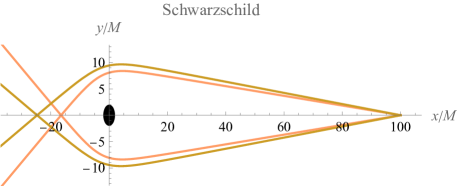
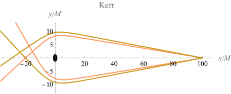
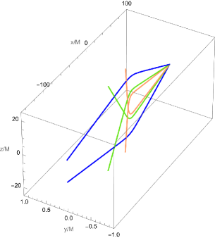
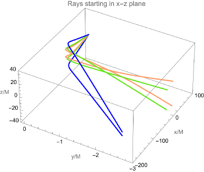
Figure 6: Gravitational light deflection (numerical results) in the Schwarzschild and in a Kerr spacetime with rotation parameter $a=S/M=0.9$. The source is at a distance $r=100M$. First row: equatorial plane; second row: light rays starting out in the $z_{O}x$ plane. Each color corresponds to a pair of rays with symmetric angles about the $x$-axis. In the Schwarzschild case, the deflection is the same for rays starting at equal (in magnitude) angles relative to the $x$-axis connecting the source and the black hole; this leads to perfectly circular Einstein rings as viewed by observers along the $x$-axis. In the Kerr spacetime, the deflection of equatorial light rays through opposite sides of the black hole differs; rays starting at equal (in magnitude) angles will not cross along the $x$-axis; and those that cross along the $x$-axis arrive at different angles. Light rays with initial direction along the $z_{O}x$ plane suffer (in addition to the convergence along the $z$-axis), a deflection along the $y$-direction. These gravitomagnetic effects do not enhance the convergence of light rays for observers along the $x$-axis (instead only slightly deforming the observed Einstein rings).

.

References

- [1] M. L. Ruggiero, A. Ortolan, and C. C. Speake, “Galactic Dynamics in General Relativity: the Role of Gravitomagnetism,” arXiv:2112.08290.
- [2] D. Astesiano and M. L. Ruggiero, “Can general relativity play a role in galactic dynamics?,” Phys. Rev. D 106 no. 12, (2022) L121501, arXiv:2211.11815.
- [3] F. I. Cooperstock and S. Tieu, “General relativity resolves galactic rotation without exotic dark matter,” arXiv:astro-ph/0507619.
- [4] J. D. Carrick and F. I. Cooperstock, “General relativistic dynamics applied to the rotation curves of galaxies,” Astrophys. Space Sci. 337 (2012) 321–329, arXiv:1101.3224.
- [5] H. Balasin and D. Grumiller, “Non-Newtonian behavior in weak field general relativity for extended rotating sources,” Int. J. Mod. Phys. D 17 (2008) 475–488, arXiv:astro-ph/0602519.
- [6] M. Crosta, M. Giammaria, M. G. Lattanzi, and E. Poggio, “On testing CDM and geometry-driven Milky Way rotation curve models with Gaia DR2,” Mon. Not. Roy. Astron. Soc. 496 no. 2, (2020) 2107–2122, arXiv:1810.04445.
- [7] D. Astesiano and M. L. Ruggiero, “Galactic dark matter effects from purely geometrical aspects of general relativity,” Phys. Rev. D 106 no. 4, (2022) 044061, arXiv:2205.03091.
- [8] L. Ciotti, “On the Rotation Curve of Disk Galaxies in General Relativity,” Astrophys. J. 936 no. 2, (2022) 180, arXiv:2207.09736.
- [9] A. N. Lasenby, M. P. Hobson, and W. E. V. Barker, “Gravitomagnetism and galaxy rotation curves: a cautionary tale,” Class. Quant. Grav. 40 (2023) 215014, arXiv:2303.06115.
- [10] K. Glampedakis and D. I. Jones, “Pitfalls in applying gravitomagnetism to galactic rotation curve modelling,” Class. Quant. Grav. 40 (2023) 147001, arXiv:2303.16679.
- [11] L. F. O. Costa, J. Natário, F. Frutos-Alfaro, and M. Soffel, “Reference frames in general relativity and the galactic rotation curves,” Phys. Rev. D 108 (2023) 044056, arXiv:2303.17516.
- [12] L. D. Landau and E. M. Lifshitz, The classical theory of fields; 4rd ed., vol. 2 of Course of theoretical physics. Butterworth-Heinemann, Oxford, UK, 1975. Trans. from the Russian.
- [13] D. Lynden-Bell and M. Nouri-Zonoz, “Classical monopoles: Newton, nut space, gravomagnetic lensing, and atomic spectra,” Rev. Mod. Phys. 70 (Apr, 1998) 427–445.
- [14] J. Natário, “Quasi-Maxwell interpretation of the spin–curvature coupling,” General Relativity and Gravitation 39 no. 9, (Sep, 2007) 1477–1487.
- [15] L. F. O. Costa and J. Natário, “Gravito-electromagnetic analogies,” General Relativity and Gravitation 46 no. 10, (2014) 1792, arXiv:1207.0465.
- [16] L. F. O. Costa, J. Natário, and N. O. Santos, “Gravitomagnetism in the Lewis cylindrical metrics,” Class. Quant. Grav. 38 no. 5, (2021) 055003, arXiv:1912.09407.
- [17] R. Gharechahi, J. Koohbor, and M. Nouri-Zonoz, “General relativistic analogs of Poisson’s equation and gravitational binding energy,” Phys. Rev. D 99 (2019) 084046.
- [18] R. T. Jantzen, P. Carini, and D. Bini, “The Many faces of gravitoelectromagnetism,” Annals Phys. 215 (1992) 1–50, arXiv:gr-qc/0106043.
- [19] D. Bini, P. Carini, and R. T. Jantzen, “The Intrinsic derivative and centrifugal forces in general relativity. 1. Theoretical foundations,” Int. J. Mod. Phys. D 6 (1997) 1–38, arXiv:gr-qc/0106013.
- [20] V. Perlick, “Gravitational lensing from a spacetime perspective,” Living Reviews in Relativity 7 (2004) 9.
- [21] V. J. Bolos, “Intrinsic definitions of ’relative velocity’ in general relativity,” Commun. Math. Phys. 273 (2007) 217–236, arXiv:gr-qc/0506032.
- [22] S. Datta and S. Mukherjee, “Possible connection between the reflection symmetry and existence of equatorial circular orbit,” Phys. Rev. D 103 no. 10, (2021) 104032, arXiv:2010.12387.
- [23] H. Stephani, D. Kramer, M. A. H. MacCallum, C. Hoenselaers, and E. Herlt, Exact solutions of Einstein’s field equations. Cambridge University Press, 2004.
- [24] A. Einstein, “Lens-like action of a star by the deviation of light in the gravitational field,” Science 84 no. 2188, (1936) 506–507.
- [25] J. Pinochet and M. V. S. Jan, “Einstein ring: weighing a star with light,” Physics Education 53 no. 5, (Jun, 2018) 055003, arXiv:1801.00001.
- [26] L. J. King et al., “A Complete infrared Einstein ring in the gravitational lens system B1938+666,” Mon. Not. Roy. Astron. Soc. 295 (1998) 41, arXiv:astro-ph/9710171.
- [27] D. J. Lagattuta, S. Vegetti, C. D. Fassnacht, M. W. Auger, L. V. E. Koopmans, and J. P. McKean, “SHARP - I. A high-resolution multiband view of the infrared Einstein ring of JVAS B1938+666,” Mon. Not. Roy. Astron. Soc. 424 no. 4, (2012) 2800–2810, arXiv:1206.1681.
- [28] V. Belokurov et al., “The Cosmic Horseshoe: Discovery of an Einstein Ring around a Giant Luminous Red Galaxy,” Astrophys. J. Lett. 671 (2007) L9, arXiv:0706.2326 [astro-ph].
- [29] C. Spiniello, L. V. E. Koopmans, S. C. Trager, O. Czoske, and T. Treu, “The X-Shooter Lens Survey - I. Dark matter domination and a Salpeter-type initial mass function in a massive early-type galaxy,” Monthly Notices of the Royal Astronomical Society 417 no. 4, (2011) 3000–3009, arXiv:1103.4773.
- [30] F. Bellagamba, N. Tessore, and R. B. Metcalf, “Zooming into the Cosmic Horseshoe: new insights on the lens profile and the source shape,” Mon. Not. Roy. Astron. Soc. 464 no. 4, (2017) 4823–4834, arXiv:1610.06003.
- [31] S. Schuldt, G. Chirivì, S. H. Suyu, A. Yıldırım, A. Sonnenfeld, A. Halkola, and G. F. Lewis, “Inner dark matter distribution of the Cosmic Horseshoe (J1148+1930) with gravitational lensing and dynamics,” Astronomy & Astrophysics 631 (2019) A40, arXiv:1901.02896.
- [32] J. Cheng, M. P. Wiesner, E.-H. Peng, W. Cui, J. R. Peterson, and G. Li, “Adaptive Grid Lens Modeling of the Cosmic Horseshoe Using Hubble Space Telescope Imaging,” Astrophys. J. 872 no. 2, (Feb., 2019) 185.
- [33] A. Durkalec, A. Pollo, U. Abbas, T.Górecki, to appear.
- [34] A. Amruth, T. Broadhurst, J. Lim, M. Oguri, G. F. Smoot, J. M. Diego, E. Leung, R. Emami, J. Li, T. Chiueh, H.-Y. Schive, M. C. H. Yeung, and S. K. Li, “Einstein rings modulated by wavelike dark matter from anomalies in gravitationally lensed images,” Nature Astronomy 7 (2023) 736–747.
- [35] T. Ono, A. Ishihara, and H. Asada, “Gravitomagnetic bending angle of light with finite-distance corrections in stationary axisymmetric spacetimes,” Phys. Rev. D 96 no. 10, (2017) 104037, arXiv:1704.05615.
- [36] M. Galoppo, S. L. Cacciatori, V. Gorini, and M. Mazza, “Equatorial Lensing in the Balasin-Grumiller Galaxy Model,” arXiv:2212.10290 [gr-qc].
- [37] A. Ishihara, Y. Suzuki, T. Ono, T. Kitamura, and H. Asada, “Gravitational bending angle of light for finite distance and the Gauss-Bonnet theorem,” Phys. Rev. D 94 no. 8, (2016) 084015, arXiv:1604.08308.
- [38] G. W. Gibbons and M. C. Werner, “Applications of the Gauss-Bonnet theorem to gravitational lensing,” Classical and Quantum Gravity 25 no. 23, (2008) 235009.
- [39] K. Jusufi, A. Övgün, J. Saavedra, Y. Vásquez, and P. A. González, “Deflection of light by rotating regular black holes using the Gauss-Bonnet theorem,” Phys. Rev. D 97 no. 12, (2018) 124024, arXiv:1804.00643.
- [40] M. Halla and V. Perlick, “Application of the Gauss–Bonnet theorem to lensing in the NUT metric,” Gen. Rel. Grav. 52 no. 11, (2020) 112, arXiv:2008.10093. [Erratum: Gen.Rel.Grav. 53, 68 (2021)].
- [41] F. C. Sánchez, A. A. Roque, B. Rodríguez, and J. Chagoya, “Total light bending in non-asymptotically flat black hole spacetimes,” Class. Quant. Grav. 41 (2024) 015019, arXiv:2306.12488.
- [42] W. Klingenberg, A Course in Differential Geometry. Graduate texts in mathematics. Springer-Verlag, 1978.
- [43] L. Godinho and J. Natário, An Introduction to Riemannian Geometry: With Applications to Mechanics and Relativity. Universitext. Springer International Publishing, 2014.
- [44] T. Damour, M. Soffel, and C.-m. Xu, “General relativistic celestial mechanics. 1. Method and definition of reference systems,” Phys. Rev. D 43 (1991) 3272–3307.
- [45] M. Soffel, “Standard relativistic reference systems and the IAU framework,” in Relativity in Fundamental Astronomy: Dynamics, Reference Frames, and Data Analysis, S. A. Klioner, P. K. Seidelmann, and M. H. Soffel, eds., vol. 261, pp. 1–6. Jan., 2010.
- [46] J. D. Kaplan, D. A. Nichols, and K. S. Thorne, “Post-Newtonian approximation in Maxwell-like form,” Phys. Rev. D 80 (2009) 124014, arXiv:0808.2510.
- [47] M. Soffel, S. Klioner, J. Muller, and L. Biskupek, “Gravitomagnetism and lunar laser ranging,” Phys. Rev. D 78 (2008) 024033.
- [48] E. Poisson and C. M. Will, Gravity: Newtonian, Post-Newtonian, Relativistic. Cambridge University Press, Cambridge, UK, 2014.
- [49] P. Mach and E. Malec, “General-relativistic rotation laws in rotating fluid bodies,” Phys. Rev. D 91 no. 12, (2015) 124053, arXiv:1501.04539.
- [50] J. Karkowski, P. Mach, E. Malec, M. Pirog, and N. Xie, “Rotating systems, universal features in dragging and antidragging effects, and bounds of angular momentum,” Phys. Rev. D 94 no. 12, (2016) 124041, arXiv:1609.06586.
- [51] H. Stephani, Relativity: An Introduction to Special and General Relativity. Cambridge University Press, 3 ed., 2004.
- [52] I. Ciufolini and J. A. Wheeler, Gravitation and Inertia. Princeton Series in Physics, Princeton, NJ, 1995.
- [53] J. Ibáñez, “Gravitational lenses with angular momentum,” Astronomy & Astrophysics 124 no. 2, (1983) 175–180.
- [54] J. Ibáñez and J. Martín, “Gravitational scattering of spinning particles: Linear approximation,” Phys. Rev. D 26 (1982) 384–389.
- [55] J. Govaerts, “The gravito-electromagnetic approximation to the gravimagnetic dipole and its velocity rotation curve,” Class. Quant. Grav. 40 no. 8, (2023) 085010, arXiv:2303.01386.
- [56] G. Clément, “The gravimagnetic dipole,” Class. Quant. Grav. 38 (2021) 075003, arXiv:2010.14473.
- [57] V. S. Manko, E. D. Rodchenko, E. Ruiz, and M. B. Sadovnikova, “Formation of a Kerr black hole from two stringy NUT objects,” Moscow Univ. Phys. Bull. 64 (2009) 359, arXiv:0901.3168.
- [58] O. James, E. von Tunzelmann, P. Franklin, and K. S. Thorne, “Gravitational lensing by spinning black holes in astrophysics, and in the movie interstellar,” Classical and Quantum Gravity 32 no. 6, (Feb, 2015) 065001.