Optical properties and exciton transfer between N-heterocyclic carbene iridium (III) complexes for blue light-emitting diode applications from first principles

Abstract

N-heterocyclic carbene (NHC) iridium (III) complexes are considered as promising candidates for blue emitters in organic light-emitting diodes. They can play the roles of the emitter as well as of electron and hole transporters in the same emission layer. We investigate optical transitions in such complexes with account of geometry and electronic structure changes upon excitation or charging and exciton transfer between the complexes from first principles. It is shown that excitation of NHC iridium complexes is accompanied by a large reorganization energy $\sim$0.7 eV and a significant loss in the oscillator strength, which should lead to low exciton diffusion. Calculations with account of spin-orbit coupling reveal a small singlet-triplet splitting $\sim$0.1 eV, whereas the oscillator strength for triplet excitations is found to be an order of magnitude smaller than for the singlet ones. The contributions of the Förster and Dexter mechanisms are analyzed via the explicit integration of transition densities. It is shown that for typical distances between emitter complexes in the emission layer, the contribution of the Dexter mechanism should be negligible compared to the Förster mechanism. On the other hand, the ideal dipole approximation, although gives the correct order of the exciton coupling, fails to reproduce the result taking into account spatial distribution of the transition density. For charged NHC complexes, we find a number of optical transitions close to the emission peak of the blue emitter with high exciton transfer rates that can be responsible for exciton-polaron quenching. The nature of these transitions is analyzed.

I Introduction

Organic semiconductors Chiang et al. (1977) are strong competitors of traditional inorganic semiconductors winning in low-cost production, easy processability, flexibility and chemical tunability Parashkov et al. (2005); Boudreault, Najari, and Leclerc (2011); Bundgaard and Krebs (2007); Shirota and Kageyama (2007). Organic light emitting diodes (OLEDs) have already become a part of our everyday life as the principal ingredient of active matrix displays and are now routinely produced at the industrial scale Forrest (2004); Hung and Chen (2002). While decisive steps have been also taken for the use of OLEDs in lighting applications, a number of problems including white light generation Sun et al. (2006); Schwartz et al. (2007); Reineke et al. (2009), roll-off of quantum efficiency at high current densities Baldo, Adachi, and Forrest (2000); Zang et al. (2008); Song et al. (2010); Wehrmeister et al. (2015); Giebink and Forrest (2008), efficient light outcoupling Lupton et al. (2000); Melpignano et al. (2006); Will et al. (2018) and long-term stability Seifert et al. (2013); Niu et al. (2017) still have to be solved.

Interaction of electrons and holes in OLEDs leads to formation of both singlet and triplet excitons. Spin statistics provides that only 25% of energy can be extracted from singlet excitons through the fluorescence process and this is the limit of the internal quantum efficiency for OLEDs based on purely organic fluorescent emitters Baldo et al. (1999); Reufer et al. (2005). It is possible, however, to take advantage of 75% of the energy left in triplet excitons through the phosphorescence processes mediated by spin-orbit coupling Baldo et al. (1998); Adachi et al. (2001a). The use of organometallic phosphors embedded as guest molecules in the emission layer of OLEDs has allowed to approach the nearly 100% internal efficiency, high luminance and long device lifetimes in the green Adachi et al. (2000) and red Adachi et al. (2001b) spectral ranges. Nevertheless, the development of stable and efficient phosphorescent blue emitters remains a challenge Erk et al. (2006); Rothmann et al. (2011); Zhang, Lee, and Forrest (2014); Niu et al. (2017).

Although OLEDs based on phosphorescent complexes have the high internal quantum efficiency, the external efficiency of such systems declines strongly with increasing the current Reineke, Walzer, and Leo (2007); Baldo, Adachi, and Forrest (2000); Song et al. (2010); Zang et al. (2008); Wehrmeister et al. (2015); Giebink and Forrest (2008). The reason is that triplet excitons have long radiative lifetimes in the microsecond range Reineke, Walzer, and Leo (2007); Baldo and Forrest (2000); Li et al. (2005); Tsuboyama et al. (2003); Lamansky et al. (2001); Giebink and Forrest (2008); Wehrmeister et al. (2015); Haneder (2009); Haneder et al. (2008); Mesta et al. (2016); van Eersel et al. (2014, 2016); Coehoorn, Bobbert, and van Eersel (2017); Coehoorn et al. (2017); de Vries et al. (2019); de Vries, Coehoorn, and Bobbert (2020); Ligthart et al. (2021, 2018); Mori et al. (2014) (as compared to nanoseconds for fluorescent dyes Giebink and Forrest (2008)) and exciton quenching through interactions with polarons Reineke, Walzer, and Leo (2007); Kalinowski et al. (2006); Song et al. (2010); Zang et al. (2008); Siboni and Aziz (2012); Mesta et al. (2016); van Eersel et al. (2014, 2016); Coehoorn, Bobbert, and van Eersel (2017); Wehrmeister et al. (2015); Ligthart et al. (2021), other excitons Reineke, Walzer, and Leo (2007); Baldo, Adachi, and Forrest (2000); Staroske et al. (2007); Song et al. (2010); Mesta et al. (2016); van Eersel et al. (2014, 2016); Coehoorn, Bobbert, and van Eersel (2017); Coehoorn et al. (2017); Wehrmeister et al. (2015); Ligthart et al. (2018); Coehoorn, Bobbert, and van Eersel (2019) and electric field Kalinowski et al. (2006) become important (see also review Murawski, Leo, and Gather (2013)). In addition to exciton loss, energy transfer to excited or charged species can provoke their dissociation and chemical degradation of the device Scholz et al. (2008); de Moraes et al. (2011); Jurow et al. (2014); Scholz et al. (2015). To improve the OLED efficiency it is, therefore, indispensable to understand the nature of optical transitions in phosphorescent complexes and microscopic mechanisms of exciton transfer. In the present paper, they are analyzed using ab initio calculations.

A low non-radiative loss of excitons and high efficiency can be expected for emitters with a short phosphorescence lifetime, which corresponds to a large spin-orbit coupling and a small singlet-triplet splitting Haneder (2009); Haneder et al. (2008). For this reason, cyclometalated octahedral iridium (III) complexes have been actively studied in the recent years Li et al. (2005); Tsuboyama et al. (2003); Lamansky et al. (2001); Adachi et al. (2001a, b, 2000); Baldo et al. (1999); de Vries et al. (2019); de Vries, Coehoorn, and Bobbert (2020); Ligthart et al. (2021, 2018); Mori et al. (2014); Coehoorn, Bobbert, and van Eersel (2019) including N-heterocyclic carbene (NHC) iridium (III) complexesSajoto et al. (2005); Schildknecht et al. (2005); Erk et al. (2006); Haneder (2009); Haneder et al. (2008). A high radiative decay rate and small singlet-triplet splittingHaneder (2009); Haneder et al. (2008) is achieved for DPBIC (Fig. 1a), which emits in the ultraviolet region. Substitution of two carbon atoms by nitrogen in each ligand (Fig. 1b) shifts the emission to the blue range, while keeping the radiative decay rate large Niu et al. (2017). This complex allows to achieve longer device lifetimes as compared to alternative blue phosphorescent emitters Niu et al. (2017). Following the OLED architecture proposed in Ref. Niu et al., 2017, we assume that the emission layer is composed of the wide band gap matrix doped with the blue phosphorescent NHC dye, which also plays the role of the electron transporter, and co-doped with DPBIC, which plays the role of the hole transporter, to guarantee the charge balance. Since there is no exciton transfer to the wide band gap matrix (as confirmed in our calculations), we investigate optical transitions in NHC dye and DPBIC complexes with account of geometry and electronic structure changes upon excitation and charging as well as exciton transfer between the complexes. This allows us to make qualitative predictions regarding the character of exciton dynamics in the emission layer and to an insight into exciton-polaron quenching.

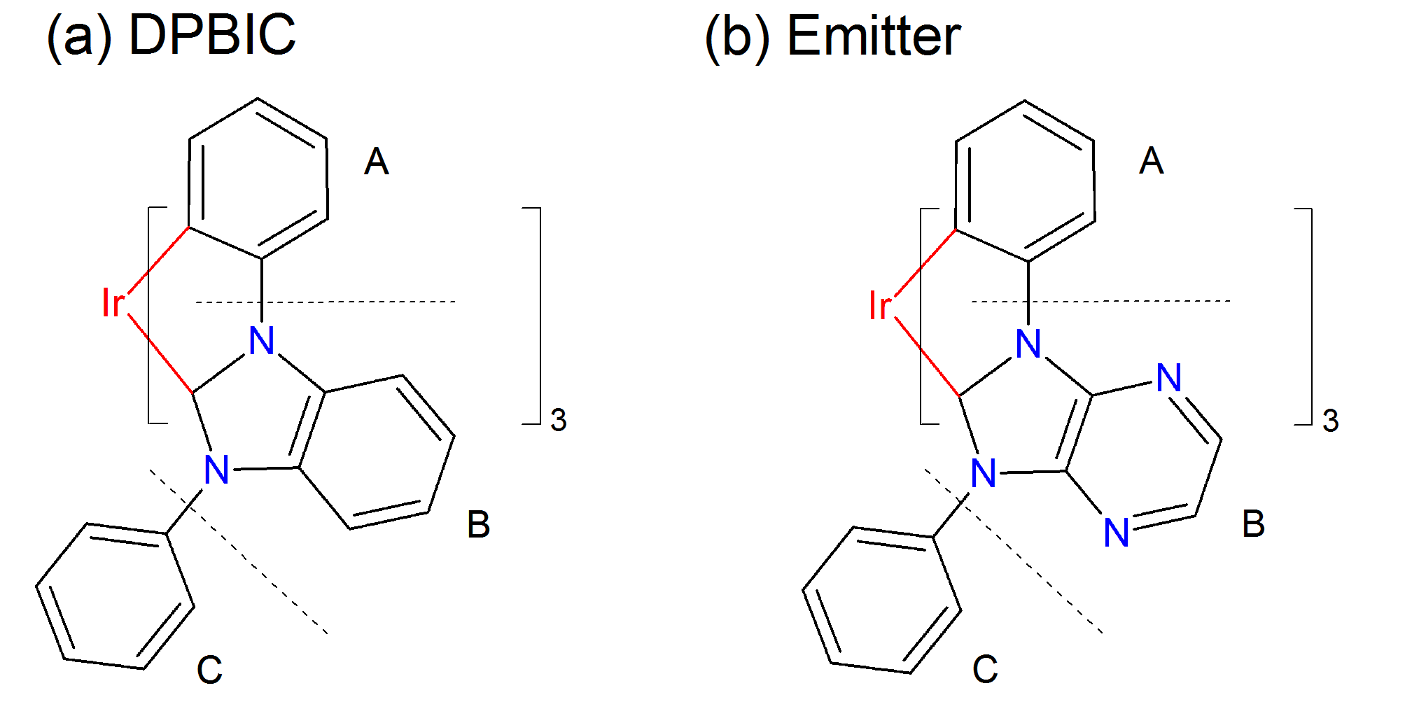
Figure 1: Chemical structure of (a) DPBIC (tris[(3-phenyl-1H-benzimidazol-1-yl-2(3H)-ylidene)-1,2-phenylene]-iridium) and (b) NHC blue emitter (tris[(3-phenyl-1H-imidazo[4,5-b]pyrazine-1-yl-2(3H)-ylidene)-1,2-phenylene]-iridium). For convenience, the fragments of the ligands are denoted as A (phenylene group), B and C (phenyl group).

The exciton transport in OLEDs is generally described using two major non-radiative energy transfer mechanisms. In the Förster model Förster (1948), the exciton transfer takes place via dipole-dipole interaction of the donor and acceptor and can be considered as the emission of a virtual photon by the donor followed by its instant re-absorption by the acceptor. The exciton coupling in the Förster model thus decays as $R_{\mathrm{DA}}^{-3}$ with the distance $R_{\mathrm{DA}}$ between the donor and acceptor. The Dexter coupling Dexter (1953) is based on the correlated transfer of two electrons due to exchange interaction and requires the spatial overlap of the donor and acceptor orbitals. It is, therefore, a short-ranged mechanism and the corresponding exciton coupling decreases exponentially with the donor-acceptor separation. While the combined spin is conserved in the Dexter mechanism making possible both triplet-triplet and singlet-singlet transport, the Förster mechanism applies only to optically-allowed transitions and triplet transport is prohibited. In materials with a large spin-orbit coupling, however, mixing between the singlet and triplet states provides that triplet transitions become optically allowed. Although their oscillator strength is still low compared to singlet ones, the triplet transport also becomes possible via the Förster mechanismBaldo and Forrest (2000). In the present paper, we analyze the contributions of these mechanisms for the exciton transfer between NHC dye complexes in the framework of time-dependent density functional theory (TDDFT). To model the dynamics of triplet excitons, the spin-orbit coupling is fully taken into account through magnetic structure calculations.

The paper is organized as follows. First the methodology for calculation of exciton coupling and transfer rates is briefly reviewed. Then we consider singlet excitations in neutral and charged DPBIC and NHC blue emitter complexes and triplet excitations of the emitter. After that, contributions of the Förster and Dexter mechanisms to the exciton transfer in a dimer of NHC blue emitter complexes are analyzed. Transfer rates for singlet and triplet transport are estimated. Finally conclusions are summarized.

II Methods

II.1 Exciton transfer mechanisms

We consider the energy transfer process

$$\mathrm{D}^{*}+\mathrm{A}\to\mathrm{A}^{*}+\mathrm{D},$$ (1)

where $\mathrm{D}$ ($\mathrm{A}$) is donor (acceptor) and the asterisk denotes the excited state. In the system we study, the donor is the NHC blue emitter and the acceptor can be another blue emitter complex, DPBIC or charged species (positively or negatively charged blue emitter or positively charged DPBIC Niu et al. (2017)).

Based on the Fermi golden rule, the rate of this process can be written as Curutchet and Mennucci (2017); Stehr et al. (2016); Hofmann, Körzdörfer, and Kümmel (2010); Förster (1948); Malic et al. (2014)

$$k=\frac{2\pi}{\hbar}|V_{\mathrm{DA}}|^{2}J_{\mathrm{DA}},$$ (2)

where $V_{\mathrm{DA}}=\langle\mathrm{DA}^{*}|V_{\mathrm{C}}|\mathrm{D}^{*}\mathrm{A}\rangle$ is the electronic coupling between the initial and final states of the system via the Coulomb interaction $V_{\mathrm{C}}$, $J_{\mathrm{DA}}$ is the spectral overlap between the normalized spectra of donor emission and acceptor absorption and $\hbar$ is the Planck constant.

Assuming that the interaction between the donor and acceptor is very weak, the wavefunctions of the initial and final states can be written through the product states of the donor and acceptor as Hofmann, Körzdörfer, and Kümmel (2010)

$$|\mathrm{D^{*}A}\rangle=\frac{1}{\sqrt{2}}\left(|\mathrm{D^{*}}\rangle|\mathrm{A}\rangle-|\mathrm{A}\rangle|\mathrm{D^{*}}\rangle\right)$$ (3)

and

$$|\mathrm{DA^{*}}\rangle=\frac{1}{\sqrt{2}}\left(|\mathrm{D}\rangle|\mathrm{A^{*}}\rangle-|\mathrm{A^{*}}\rangle|\mathrm{D}\rangle\right).$$ (4)

Correspondingly the coupling is split into two components $V_{\mathrm{DA}}=V_{\mathrm{F}}+V_{\mathrm{D}}$ Curutchet and Mennucci (2017); Stehr et al. (2016); Hofmann, Körzdörfer, and Kümmel (2010); Malic et al. (2014), where

$$V_{\mathrm{F}}=e^{2}\int\int\mathrm{d}\mathbf{r}\mathrm{d}\mathbf{r}^{\prime}\frac{\rho^{\mathrm{T}*}_{\mathrm{A}}(\mathbf{r})\rho^{\mathrm{T}}_{\mathrm{D}}(\mathbf{r}^{\prime})}{|\mathbf{r}-\mathbf{r}^{\prime}|}$$ (5)

corresponds to the Förster energy transfer Förster (1948) and

$$V_{\mathrm{D}}=-e^{2}\sum_{\sigma,\sigma^{\prime}}\int\int\mathrm{d}\mathbf{r}\mathrm{d}\mathbf{r}^{\prime}\frac{\gamma^{\mathrm{T}*}_{\mathrm{A},\sigma\sigma^{\prime}}(\mathbf{r},\mathbf{r}^{\prime})\gamma^{\mathrm{T}}_{\mathrm{D},\sigma\sigma^{\prime}}(\mathbf{r},\mathbf{r}^{\prime})}{|\mathbf{r}-\mathbf{r}^{\prime}|}$$ (6)

describes the Dexter energy transfer Dexter (1953). Here $\mathbf{r}$ and $\mathbf{r}^{\prime}$ are real-space vectors, $\sigma$ and $\sigma^{\prime}$ correspond to spin up ($\uparrow$) or spin down ($\downarrow$) and $e$ is the elementary charge. We also introduce here the notations for the transition density matrix related to the excited and ground-state wavefunctions $\Psi_{\mathrm{e}}$ and $\Psi_{\mathrm{g}}$, respectively, as

$$\begin{split}\gamma^{\mathrm{T}}_{\sigma\sigma^{\prime}}&(\mathbf{r},\mathbf{r}^{\prime})=N\sum_{\sigma_{2},\sigma_{3},...,\sigma_{N}}\int...\int\mathrm{d}\mathbf{r}_{2}\mathrm{d}\mathbf{r}_{3}...\mathrm{d}\mathbf{r}_{N}\\ &\Psi^{*}_{\mathrm{e}}(\sigma\mathbf{r},\sigma_{2}\mathbf{r}_{2},...,\sigma_{N}\mathbf{r}_{N})\Psi_{\mathrm{g}}(\sigma^{\prime}\mathbf{r}^{\prime},\sigma_{2}\mathbf{r}_{2},...,\sigma_{N}\mathbf{r}_{N}),\end{split}$$ (7)

and transition density $\rho^{\mathrm{T}}(\mathbf{r})=\sum_{\sigma}\gamma_{\sigma\sigma}^{\mathrm{T}}(\mathbf{r},\mathbf{r})$. As reflected in Eqs. (5) and (6), only optically allowed transitions are involved in the Förster mechanism, while spin flip is possible in the Dexter mechanism. It is also seen from Eq. (6) that the Dexter mechanism depends on the overlap of the donor and acceptor states and, therefore, falls exponentially upon increasing the distance between them.

Assuming that the size of the donor and acceptor molecules is small compared to the distance $R=|\mathbf{R}|$ between their centers of mass, Eq. (5) can be expanded to powers of $R^{-1}$ (Ref. Hofmann, Körzdörfer, and Kümmel, 2010) and the first term of this expansion is given by

$$V_{\mathrm{F}}^{\mathrm{IDA}}=\kappa_{\mathrm{AD}}\frac{d^{\mathrm{T}*}_{\mathrm{A}}d^{\mathrm{T}}_{\mathrm{D}}}{R^{3}}.$$ (8)

Here

$$\mathbf{d}^{\mathrm{T}}=-e\int\mathrm{d}\mathbf{r}\rho^{\mathrm{T}}(\mathbf{r})\mathbf{r}$$ (9)

is the transition dipole moment, $d^{\mathrm{T}}=|\mathbf{d}^{\mathrm{T}}|$ and

$$\kappa_{\mathrm{AD}}=\mathbf{e}_{\mathrm{A}}\mathbf{e}_{\mathrm{D}}-3\frac{(\mathbf{e}_{\mathrm{A}},\mathbf{R})(\mathbf{e}_{\mathrm{D}},\mathbf{R})}{R^{2}}$$ (10)

is the factor describing the relative orientation of unit dipole moments $\mathbf{e}=\mathbf{d}^{\mathrm{T}}/d^{\mathrm{T}}$. Eq. (8) simply corresponds to the dipole-dipole coupling of the transition dipole moments of the donor and acceptor and is referred to below as the ideal dipole approximation (IDA).

II.2 Exciton coupling from TDDFT

The large size of the iridium complexes combined with the necessity of taking into account spin-orbit coupling makes ab initio calculations of their optical properties computationally expensive. Therefore, in the present paper we use time-dependent density functional theory (TDDFT) Marques et al. (2012); Ullrich (2012); Castro et al. (2004); Marques and Gross (2004); Marques et al. (2006), which provides a sufficient accuracy at a moderate computational cost.

In TDDFT Marques et al. (2012); Ullrich (2012), the time-dependent Kohn-Sham equations Runge and Gross (1984) are considered:

$$i\hbar\frac{\partial}{\partial t}\phi_{m\sigma}\left(\mathbf{r},t\right)=H_{KS,\sigma\sigma^{\prime}}\left(\mathbf{r},t\right)\phi_{m\sigma^{\prime}}\left(\mathbf{r},t\right),$$ (11)

where $t$ is time, $\phi_{m\sigma}$ is the component of the Kohn-Sham wavefunction of one-particle state $m$ corresponding to spin $\sigma$ and $H_{KS}$ is the Kohn-Sham Hamiltonian including the kinetic energy, external potential $v_{\mathrm{ext}}$ describing electron interactions with ions and external fields and Hartree, $v_{\mathrm{H}}$, and exchange-correlation, $v_{\mathrm{xc}}$, terms describing interactions between electrons:

$$\begin{split}H_{KS,\sigma\sigma^{\prime}}=&-\frac{\hbar^{2}}{2m_{e}}\nabla^{2}\delta_{\sigma\sigma^{\prime}}+v_{\mathrm{ext},\sigma\sigma^{\prime}}(\mathbf{r},t)\\ &+v_{\mathrm{H}}(\mathbf{r},t)\delta_{\sigma\sigma^{\prime}}+v_{\mathrm{xc},\sigma\sigma^{\prime}}(\mathbf{r},t).\end{split}$$ (12)

Here $m_{e}$ is the electron mass and $\delta_{\sigma\sigma^{\prime}}$ is the Kronecker delta.

The Kohn-Sham wavefunctions provide no information on the real wavefunctions of the system. Nevertheless, they allow to reconstruct the real electron density. In the general non-collinear case, the spin density is introduced as

$$n_{\sigma\sigma^{\prime}}(\mathbf{r},t)=\sum_{m}^{\mathrm{occ}}\phi_{m\sigma}^{*}\left(\mathbf{r},t\right)\phi_{m\sigma^{\prime}}\left(\mathbf{r},t\right).$$ (13)

and the Hartree and exchange-correlation terms are considered as functionals of this density.

Following this logic, an analogue of the Dexter exciton coupling from Eq. 6 for TDDFT can be proposed in the form

$$\begin{split}V_{\mathrm{D}}=e^{2}\sum_{\sigma,\sigma^{\prime},\tau,\tau^{\prime}}&\int\int\mathrm{d}\mathbf{r}\mathrm{d}\mathbf{r}^{\prime}\rho^{\mathrm{T*}}_{\mathrm{A,\sigma\sigma^{\prime}}}(\mathbf{r})\\ &\times g_{\mathrm{xc},\sigma\sigma^{\prime}\tau\tau^{\prime}}(\mathbf{r},\mathbf{r}^{\prime})\rho^{\mathrm{T}}_{\mathrm{D,\tau\tau^{\prime}}}(\mathbf{r}^{\prime}),\end{split}$$ (14)

where $\rho^{\mathrm{T}}_{\mathrm{\sigma\sigma^{\prime}}}(\mathbf{r})=\gamma^{\mathrm{T}}_{\mathrm{\sigma\sigma^{\prime}}}(\mathbf{r},\mathbf{r})$ and

$$g_{\mathrm{xc},\sigma\sigma^{\prime}\tau\tau^{\prime}}(\mathbf{r},\mathbf{r}^{\prime})=\frac{\delta v_{\mathrm{xc},\sigma\sigma^{\prime}}(\mathbf{r})}{\delta n_{\tau\tau^{\prime}}(\mathbf{r}^{\prime})}$$ (15)

is the exchange-correlation kernel.

In the present paper, however, we limit consideration of the Dexter mechanism to singlet excitons without account of spin-orbit coupling when $g_{\mathrm{xc},\sigma\sigma^{\prime}\tau\tau^{\prime}}=g_{\mathrm{xc},\sigma\tau}\delta_{\sigma\sigma^{\prime}}\delta_{\tau\tau^{\prime}}$ and the corresponding exciton coupling is given by:

$$V_{\mathrm{D}}=e^{2}\int\int\mathrm{d}\mathbf{r}\mathrm{d}\mathbf{r}^{\prime}\rho^{\mathrm{T*}}_{\mathrm{A}}(\mathbf{r})g_{\mathrm{xc}}(\mathbf{r},\mathbf{r}^{\prime})\rho^{\mathrm{T}}_{\mathrm{D}}(\mathbf{r}^{\prime}),$$ (16)

where $g_{\mathrm{xc}}=(g_{\mathrm{xc},\uparrow\uparrow}+g_{\mathrm{xc},\uparrow\downarrow})/2$. This expression was formally proved in paper Hsu et al. (2001). Note that we neglect the overlap between the donor and acceptor transition densities Curutchet and Mennucci (2017); Mennucci and Curutchet (2011); Hsu et al. (2001).

Therefore, in TDDFT, both the Dexter and Förster contributions to the exciton coupling are determined by the transition densities $\rho^{\mathrm{T}}_{\mathrm{A}}$ and $\rho^{\mathrm{T}}_{\mathrm{D}}$ of the acceptor and donor. For the IDA coupling described by Eq. (8), it is sufficient to know the transition dipole moments. Since the ground and excited-state wavefunctions are not known in TDDFT, these quantities are not accessible directly from Eqs. (7) and (9). However, as it turns out Thiele and Kümmel (2009); Hofmann and Kümmel (2012); Fischer, Cramer, and Govind (2015); Schelter and Kümmel (2018); Jornet-Somoza and Lebedeva (2019), they can be extracted from the linear-response calculations.

The linear response $\delta n(\mathbf{r},t)=\sum_{\sigma}\delta n_{\sigma\sigma}(\mathbf{r},t)$ of the charge density to an external potential $\delta v_{\mathrm{ext}}(\mathbf{r}^{\prime},t^{\prime})=\sum_{\sigma}\delta v_{\mathrm{ext},\sigma\sigma}(\mathbf{r},t)$ is determined by the density response function $\chi(\mathbf{r},\mathbf{r}^{\prime},t-t^{\prime})$ Marques et al. (2012); Ullrich (2012):

$$\delta n(\mathbf{r},t)=\sum\int\mathrm{d}t^{\prime}\int\mathrm{d}\mathbf{r}^{\prime}\chi(\mathbf{r},\mathbf{r}^{\prime},t-t^{\prime})\delta v_{\mathrm{ext}}(\mathbf{r}^{\prime},t^{\prime}),$$ (17)

which in the frequency domain corresponds to

$$\begin{split}\delta n(\mathbf{r},\omega)=\int\mathrm{d}\mathbf{r}^{\prime}\chi(\mathbf{r},\mathbf{r}^{\prime},\omega)\delta v_{\mathrm{ext}}(\mathbf{r}^{\prime},\omega).\end{split}$$ (18)

The density response function can be written in the Lehmann representation Marques et al. (2012); Ullrich (2012) as

$$\begin{split}\chi=\frac{1}{\hbar}\lim_{\eta\to+0}&\sum_{m=1}^{\infty}\Bigg{(}\frac{\langle 0|\hat{n}(\mathbf{r})|m\rangle\langle m|\hat{n}(\mathbf{r}^{\prime})|0\rangle}{\omega-\Omega_{m}+i\eta}\\ &-\frac{\langle 0|\hat{n}(\mathbf{r}^{\prime})|m\rangle\langle m|\hat{n}(\mathbf{r})|0\rangle}{\omega+\Omega_{m}+i\eta}\Bigg{)},\end{split}$$ (19)

where $|m\rangle$ denotes the $m$-th excited state wavefunction, $|0\rangle$ is the ground state wavefunction, $\Omega_{m}$ is the frequency of the $n$-th excitation and $\hat{n}(\mathbf{r})=\sum_{N}\delta(\mathbf{r}-\mathbf{r}_{i})$ is the density operator.

The resonant part of the density response function thus reads

$$\begin{split}\chi^{\mathrm{res}}=-\frac{i\pi}{\hbar}\sum_{m=1}^{\infty}&f_{0}(\omega-\Omega_{m})\langle 0|\hat{n}(\mathbf{r})|m\rangle\langle m|\hat{n}(\mathbf{r}^{\prime})|0\rangle,\end{split}$$ (20)

where $f_{0}(\omega)=\delta(\omega)$ is the normalized lineshape. Note that when spin-orbit coupling is not taken into account and the matrix elements above are real, this resonant part exactly corresponds to the imaginary part of the response function: $\chi^{\mathrm{res}}=i\mathrm{Im}\ \chi$ (see Eq. (19)).

Based on Eqs. (18) and (20), the resonant part of the linear response of the charge density $\delta n$ to the small electric field $\delta\mathbf{E}$ at frequency $\omega$ can be written as

$$\begin{split}\delta n^{\mathrm{res}}(\mathbf{r},\omega)=&\frac{i\pi}{\hbar}\sum_{\mu=1}^{3}\sum_{m=1}^{\infty}\delta E_{\mu}f_{0}(\omega-\Omega_{m})\times\\ &\int\mathrm{d}\mathbf{r}^{\prime}\langle 0|\hat{n}(\mathbf{r})|m\rangle\langle m|\hat{d}_{\mu}(\mathbf{r}^{\prime})|0\rangle,\end{split}$$ (21)

where $\hat{\mathbf{d}}(\mathbf{r})=-e\mathbf{r}\hat{n}(\mathbf{r})$ is the dipole moment operator. The first-order derivative with respect to the electric field $\tilde{n}^{\mathrm{res}}_{\mu}=\partial n^{\mathrm{res}}/\partial E_{\mu}$ then takes the form

$$\tilde{n}^{\mathrm{res}}_{\mu}(\mathbf{r},\omega)=\frac{i\pi}{\hbar}\sum_{m=1}^{\infty}f_{0}(\omega-\Omega_{m})\rho^{\mathrm{T*}}_{m}(\mathbf{r})d_{m,\mu}^{\mathrm{T}},$$ (22)

where $\mathbf{d}^{\mathrm{T}}_{m}=\int\mathrm{d}\mathbf{r}\langle m|\hat{\mathbf{d}}(\mathbf{r})|0\rangle$ is the transition dipole moment for the $m$-th excited state and $\rho^{\mathrm{T}}_{m}(\mathbf{r})=\langle m|\hat{n}(\mathbf{r})|0\rangle$ is the corresponding transition density. The transition density can thus be found from the linear response of the charge density close to the resonance once the transition dipole moment is known

$$\rho^{\mathrm{T*}}_{m}(\mathbf{r})=-\frac{i\hbar}{\pi f_{0}(0)}\sum_{\mu=1}^{3}\frac{\tilde{n}^{\mathrm{res}}_{\mu}(\mathbf{r},\Omega_{m})e_{m,\mu}^{\mathrm{T}}}{|\mathbf{d}_{m}^{\mathrm{T}}|}.$$ (23)

Here, as before, $\mathbf{e}_{m}=\mathbf{d}_{m}/|\mathbf{d}_{m}^{\mathrm{T}}|$. Again, when spin-orbit coupling is not taken into account, $\tilde{n}_{\mu}^{\mathrm{res}}=i\mathrm{Im}\ \tilde{n}_{\mu}$.

The polarizability corresponds to the linear response of the dipole moment and its resonant part is given by

$$\begin{split}\alpha^{\mathrm{res}}_{\nu\mu}(\omega)&=\partial d^{\mathrm{res}}_{\nu}/\partial E_{\mu}=-e\int\mathrm{d}\mathbf{r}x_{\nu}\tilde{n}^{\mathrm{res}}_{\mu}(\mathbf{r},\omega)\\ &=\frac{i\pi}{\hbar}\sum_{m=1}^{\infty}f_{0}(\omega-\Omega_{m})d_{m,\nu}^{\mathrm{T*}}d_{m,\mu}^{\mathrm{T}}.\end{split}$$ (24)

Therefore, transition dipole moments can be found from the polarizability tensor.

Irrespective of whether spin-orbit coupling is taken into account or no, the resonance part of the diagonal elements of the polarizability corresponds to the imaginary part of these elements: $\alpha^{\mathrm{res}}_{\nu\mu}\delta_{\nu\mu}=i\mathrm{Im}\ \alpha_{\nu\mu}\delta_{\nu\mu}$. The same also holds for the trace of the polarizability:

$$\begin{split}\frac{1}{3}\mathrm{Im}[\mathrm{Tr}\alpha(\omega)]&=\frac{\pi}{3\hbar}\sum_{m=1}^{\infty}f_{0}(\omega-\Omega_{m})|\mathbf{d}_{m}^{\mathrm{T}}|^{2}\\ &=\frac{\pi}{2}\frac{e^{2}}{m_{e}}\sum_{m=1}^{\infty}\frac{f_{m}}{\Omega_{m}}f_{0}(\omega-\Omega_{m}),\end{split}$$ (25)

where $f_{m}$ is the oscillator strength of the $m$-th excitation. The latter can be used to compute the magnitudes of transition dipole moments, while diagonalization of the polarizability tensor allows to establish the directions of transition dipole moments. As soon as the transition dipole moments are known, Eq. (23) can be used to find the transition densities and Eqs. (5), (16) and (8) to compute the exciton coupling.

II.3 Transfer rate

The exciton transfer rate $k$ are computed according to Eq. (2). Two approaches are used to estimate the spectral overlap $J_{\mathrm{DA}}$.

The first one is the Marcus rate expression Marcus (1956, 1993); Stehr et al. (2016):

$$J_{\mathrm{M}}=\sqrt{\frac{1}{4\pi\lambda k_{\mathrm{B}}T}}\exp{\left(-\frac{\Delta^{2}}{4\lambda k_{\mathrm{B}}T}\right)}.$$ (26)

Here $\lambda$ is the reorganization energy, $\Delta=\lambda+\Delta G=\hbar(\Omega_{\mathrm{D}}-\Omega_{\mathrm{A}})$ is the energy shift in the emission peak of the donor and absorption peak of the acceptor with $\Delta G$ being the free energy difference between the final and initial states of the system, $T$ is temperature and $k_{\mathrm{B}}$ is the Boltzmann constant. The reorganization energy, $\lambda$, can be divided into the contributions associated with geometry relaxation of the ground state, $\lambda_{\mathrm{gr}}$, and of the excited state, $\lambda_{\mathrm{ex}}$, so that $\lambda=\lambda_{\mathrm{gr}}+\lambda_{\mathrm{ex}}$ Stehr et al. (2016). These two contributions are related to the structural rearrangements of the donor and acceptor upon the exciton transfer, respectively.

The Marcus rate expression is valid in the classical limit $k_{\mathrm{B}}T\geq\hbar\omega$, when vibrations can be treated classically. However, at room temperature, not all vibrations can be described in this way. To check how these vibrations affect the transfer rates, we consider the Levith-Jortner expression Levich and Dogonadze (1959); Levich (1966); Jortner (1976); Stehr et al. (2016), where the vibrations that cannot be treated classically are taken into account through the effective frequency $\omega_{\mathrm{eff}}$, Huang-Rhys factor $S_{\mathrm{eff}}$ and quantum reorganization energy $\lambda_{\mathrm{q}}=\hbar\omega_{\mathrm{eff}}S_{\mathrm{eff}}=\lambda-\lambda_{\mathrm{c}}$ ($\lambda_{\mathrm{c}}$ is the classical contribution to the reorganization energy):

$$\begin{split}&J_{\mathrm{LH}}=\sqrt{\frac{1}{4\pi\lambda_{\mathrm{c}}k_{\mathrm{B}}T}}\times\\ &\sum_{p}\frac{S_{\mathrm{eff}}^{p}}{p!}\exp{\left(-S_{\mathrm{eff}}\right)}\exp{\left(-\frac{(\Delta-\lambda_{\mathrm{q}}+p\hbar\omega_{\mathrm{eff}})^{2}}{4\lambda_{c}k_{\mathrm{B}}T}\right)}.\end{split}$$ (27)

The parameters for this expression are estimated from the vibronic structure of the experimental photoluminescence spectrum of DPBIC at temperature 77 K Erk et al. (2006) (Fig. 2). The energy corresponding to the effective frequency of the vibrations coupled to the excitation, $\hbar\omega_{\mathrm{eff}}$, is found to be about 0.138 eV from the energy gap between the first and second peaks in the spectra Wang, Guerzo, and Schmehl (2004). This energy is in the range of values of 0.08 – 0.14 eV obtained for other iridium complexes de Vries et al. (2019). The values of $\lambda_{\mathrm{q,gr}}\approx 0.10$ eV and $S_{\mathrm{eff,gr}}=\lambda_{\mathrm{q,gr}}/(\hbar\omega_{\mathrm{eff}})\approx 0.73$ are obtained by fitting the photoluminescence spectrum assuming that the density of states for the donor is described by the equation similar to Eq. (27) (Ref. Stehr et al., 2016). Using the same quantum contribution to the reorganization energy for the acceptor, $\lambda_{\mathrm{q,ex}}=\lambda_{\mathrm{q,gr}}=\lambda_{\mathrm{q}}/2$, we get total $\lambda_{\mathrm{q}}=0.20$ eV and $S_{\mathrm{eff}}=1.46$. Note that at 300 K, the vibronic structure of the photoluminescence spectrumHaneder et al. (2008); Haneder (2009) is not resolved and the shape of the spectrum approaches that described by the classical Marcus rate expression (Fig. 2). Such a qualitative change in the spectrum shape is reproduced using the estimated parameters.

When several optical transitions are involved in the exciton transfer, the characteristic total transfer rate is estimated from the rates of these transitions, $k_{i}$, as

$$k_{\mathrm{tot}}=\left(\sum_{i}k_{i}^{2}\right)^{1/2}.$$ (28)

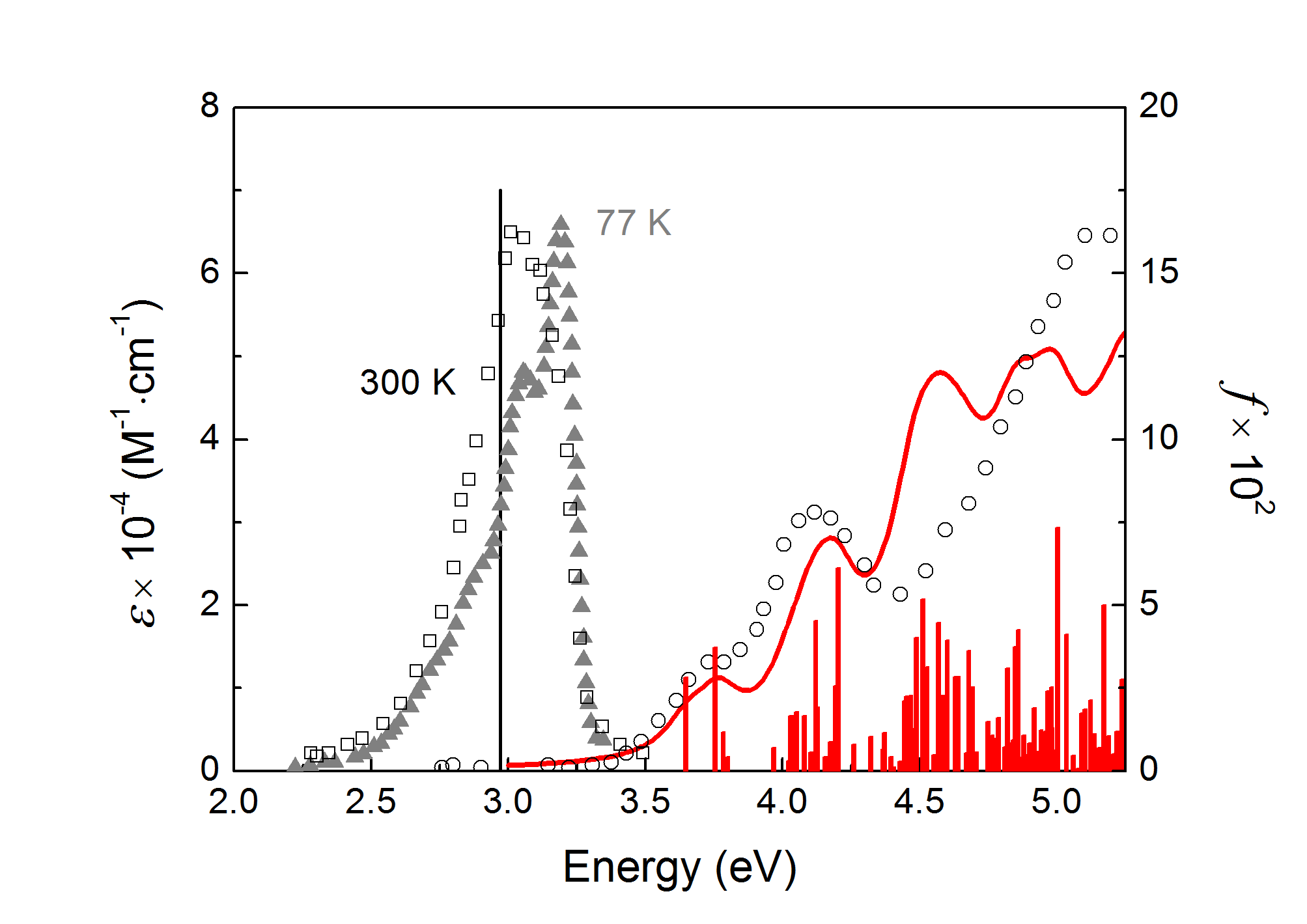
Figure 2: Calculated molar extinction coefficient $\epsilon$ (red line, in M${}^{-1}\cdot$cm^-1, left axis) and oscillator strength $f$ of optical transitions (red bars, right axis) for DPBIC as functions of the excitation energy (in eV). The energy corresponding to fluorescence is indicated by the vertical black line. The experimental data Haneder (2009) for the absorption spectrum of DPBIC in the polymethylmethacrylate matrix are shown by circles. Experimental photoluminescence spectra at temperatures 77 K Erk et al. (2006) and 300 K Haneder et al. (2008); Haneder (2009) are shown in arbitrary units by triangles and squares, respectively. The molar extinction coefficient is found from Eq. (30) using the solution of the Casida equation without account of spin-orbit coupling for isolated DPBIC with the PBE0 functional, def2-TZVP basis set and def2/J auxiliary basis set. Lorentzian broadening with half width at half maximum of 0.1 eV is applied. The matrix refractive index is taken equal to 1.5 (polymethylmethacrylate).

II.4 Computational details

II.4.1 Casida equation

To compute absorption spectra and transition dipole moments of isolated species as well as to perform geometry optimization of the first excited states, we use the Casida equation Casida (2011). In this approach, poles and residues of the first-order response function are found by solving the eigenvalue problem in the basis of particle-hole states.

The polarizability is obtained from excitation frequencies and oscillator strengths according to Eq. (25). The absorption cross-section is related to the polarizability as

$$\sigma(\omega)=\frac{4\pi\omega}{3c}\mathrm{Im}[\mathrm{Tr}\alpha(\omega)],$$ (29)

where $c$ is the speed of light, and the molar extinction coefficient for molecules in a matrix is computed as

$$\epsilon(\omega)=\frac{4\pi\omega N_{\mathrm{A}}}{3n_{\mathrm{M}}c\ln{10}}\mathrm{Im}[\mathrm{Tr}\alpha(\omega)],$$ (30)

where $N_{\mathrm{A}}$ is the Avogadro constant and $n_{\mathrm{M}}$ is the matrix refractive index.

We take the advantage of the efficient implementation of the Casida equation in the ORCA code Neese (2012, 2018) based on atom localized basis sets. Balanced polarized triple-zeta basis sets (def2-TZVP) Weigend and Ahlrichs (2005) and auxiliary basis sets def2/J Weigend (2006) are employed. All electrons are explicitly considered for hydrogen, nitrogen and carbon, while for iridium the quasirelativistic pseudopotential Andrae et al. (1990) is used to replace the core electrons with an effective core potential. The hybrid PBE0 exchange-correlation functional Adamo and Barone (1999) is applied. The use of the hybrid functional allows us to improve description of excitation energies and oscillator strengths as compared to the results obtained in the local density approximation (LDA) Ceperley and Alder (1980) and generalized gradient approximation (GGA) with the exchange-correlation functional of Perdew, Burke and Ernzerhof (PBE) Perdew, Burke, and Ernzerhof (1996) (see Supplementary Information). The resolution of identity (RI) approximation Eichkorn et al. (1995) for evaluation of the Coulomb terms and “chain of spheres exchange" (COSX) algorithm Neese et al. (2009) for the calculation of the exchange terms (together RIJCOSX Petrenko, Kossmann, and Neese (2011)) are applied to reduce the computational cost. The single-point energies are converged in self-consistent field calculations within $3\cdot 10^{-7}$ eV. The geometry optimization is performed with the quasi-Newton optimizer using the Broyden-Fletcher-Goldfarb-Shanno (BFGS) update. The forces are converged within $2\cdot 10^{-2}$ eV/Å. The Casida equation Casida (2011) is solved in the Tamm-Dancoff approximation Hirata and Head-Gordon (1999). The Davidson diagonalization procedure Hsu, Davidson, and Pitzer (1976) is used. The convergence tolerance for the energies is $10^{-5}$ eV.

II.4.2 Real-time propagation

The Casida equation provides an efficient tool for calculation of transition dipole moments of isolated species for singlet excitations. This method, however, is based on the use of real wavefunctions and this excludes the possibility of consideration of non-collinear spins. Furthermore, it is not straightforward to decompose the total response into contributions from different spatial domains in this case. To study exciton transfer in supramolecular systems in the present paper, we use the real-time propagation approach as implemented in the Octopus code Marques et al. (2003); Castro et al. (2006); Andrade et al. (2015); Castro, Marques, and Rubio (2004). The advantage of this method is that the corresponding routines are massively parallelized Andrade et al. (2012) and do not require computation of virtual states.

In real-time propagation, the time-dependent Kohn-Sham equations (11)–(13) are solved by explicit integration in time. Initially the system in the ground state is considered. An infinitesimal electric field pulse $\delta E_{\mu}(t)=\kappa_{\mu}\delta(t)$, where $\delta(t)$ is the delta function, is applied to simulate the dipole response. The pulses in three orthogonal directions are studied to extract the full polarizability tensor. The time-dependent dipole moment along the axis $\nu$ is found from the response of the electron density determined by Eq. (13) as

$$d_{\nu}(t)=-e\sum_{\sigma}\int d\mathbf{r}x_{\nu}n_{\sigma\sigma}(\mathbf{r},t),$$ (31)

The Fourier transform of the time-dependent dipole moment gives the polarizability

$$\alpha_{\nu\mu}(\omega)=\frac{1}{\kappa_{\mu}}\int_{0}^{\infty}dte^{-i\omega t}(d_{\nu}(t)-d_{\nu}(0)).$$ (32)

To extract the contributions of individual molecules to the total absorption spectrum as well transition densities and transition dipole moments for each of them, the system is decomposed into local domains Jornet-Somoza et al. (2015); Jornet-Somoza and Lebedeva (2019). The partitioning is performed on the basis of the quantum theory of atoms in molecules (QTAIM) Bader (1994). According to this theory, different regions of space are assigned to specific atoms following the gradient of the electron density. The calculations of time-dependent dipole moments, polarizabilities and cross-sections can then be performed within each local domain according to Eqs. (31)–(29).

The individual transition dipole moments computed in this way are used to obtain the IDA exciton coupling with account of the effects of the local chemical environment Jornet-Somoza and Lebedeva (2019) according to Eq. (8). The individual transition densities are used to evaluate the exciton coupling with account of multipoles beyond the dipole-dipole term according to Eqs. (5) and (16). Following the transition density cube method (TDCM) Krueger, Scholes, and Fleming (1998); Curutchet and Mennucci (2017); Jornet-Somoza and Lebedeva (2019), integration is performed explicitly on a three-dimensional real-space grid by summing up contributions from finite-size volume elements.

Gaussian broadening is applied in real-time propagation calculations. The corresponding lineshape is given by

$$f_{0}^{\mathrm{G}}(\omega)=\frac{1}{\sqrt{2\pi}\Gamma}\mathrm{exp}\left[-\frac{\omega^{2}}{2\Gamma^{2}}\right],$$ (33)

where $\Gamma$ is expressed through the half width at half maximum as $\Gamma=\mathrm{HWHM}/\sqrt{2\mathrm{ln}2}$. The peak height in this case is given by $f_{0}^{\mathrm{G}}(0)=1/(\sqrt{2\pi}\Gamma)$.

In the Octopus code Marques et al. (2003); Castro et al. (2006); Andrade et al. (2015); Castro, Marques, and Rubio (2004), one-particle wavefunctions and electron density are discretized on a dense real-space regular grid. The minimum mesh consisting of spheres around each atom is used in the present paper. The grid spacing of 0.14 Å and spheres around each atom of the radius of 3.5 Å are sufficient to converge the excitation energies within the accuracy of 0.1 eV. The LDA functional Perdew and Zunger (1981) is used. The relativistic separable pseudopotentials of Hartwigsen, Goedecker and Hutter Hartwigsen, Goedecker, and Hutter (1998) are applied to enable calculations with account of spin-orbit coupling. Note that although the excitation energies are strongly underestimated within LDA, the calculated spectra are qualitatively similar to those obtained with the PBE0 functional (see Supplementary Information). Therefore, LDA can be used to qualitatively study exciton dynamics. The conjugate-gradients solverJiang, Baranger, and Yang (2003) with a mixing parameter of 0.3 is used for the ground-state calculation of eigenstates with the relative tolerance of $10^{-11}$. The approximately enforced time-reversal symmetry (AERTS) propagator Castro, Marques, and Rubio (2004) is used to integrate Kohn-Sham equations (11) in time. The time step is 0.79 as. The propagation time is almost 200 fs. The strength of the electric field pulse is $\kappa_{\mu}=\kappa=0.001$ Å^-1. This strength is small enough to stay in the linear-response regime. The electronic density is saved every 100 time steps.

II.4.3 Sternheimer equation

A clear advantage of the real-time propagation approach is that the optical response is obtained for all frequencies at once. The linewidth, however, is determined by the propagation time and long simulation times are required to resolve strongly overlapping bands. Resolving triplet peaks located in the close vicinity of singlet ones with a large oscillator strength can be particularly challenging.

The calculation of absorption spectra with account of spin-orbital coupling within narrow spectral regions is performed in the present paper based on the Sternheimer equation Bitzek et al. (2006); Andrade et al. (2007); Strubbe (2012); Strubbe et al. (2012); Andrade et al. (2015); Lebedeva et al. (2019) for the first-order derivatives of Kohn-Sham states $\tilde{\phi}_{m\sigma,\mu}=\partial\phi_{m\sigma}/\partial E_{\mu}$ with respect to the electric field:

$$\begin{split}\big{(}(\pm\omega+&i\eta-\epsilon_{0,m})\delta_{\sigma\sigma^{\prime}}+H_{0,\sigma\sigma^{\prime}}(\mathbf{r})\big{)}\tilde{\phi}_{m\sigma^{\prime},\mu}(\mathbf{r},\pm\omega)\\ &=-P_{c}\tilde{H}_{\sigma\sigma^{\prime},\mu}(\mathbf{r},\pm\omega)\phi_{0,m\sigma^{\prime}}(\mathbf{r}).\end{split}$$ (34)

Here $H_{0,\sigma\sigma^{\prime}}$ is the unperturbed Hamiltonian, $\epsilon_{0,m}$ is the energy of the unperturbed $m$-th Kohn-Sham state, $P_{c}$ is the projector onto the unoccupied states, $i\eta$ is a small but finite imaginary frequency added to avoid divergences at the resonances Andrade et al. (2007); Strubbe (2012); Strubbe et al. (2012); Andrade et al. (2015) and $\tilde{H}_{\sigma\sigma^{\prime},\mu}$ is the first-order derivative of the Hamiltonian:

$$\begin{split}\tilde{H}_{\sigma\sigma^{\prime},\mu}&(\mathbf{r},\omega)=-ex_{\mu}\delta_{\sigma\sigma^{\prime}}+e^{2}\sum_{\tau,\tau^{\prime}}\int d\mathbf{r^{\prime}}\\ &\tilde{n}_{\tau\tau^{\prime},\mu}(\mathbf{r^{\prime}},\omega)\left(\frac{\delta_{\sigma\sigma^{\prime}}\delta_{\tau\tau^{\prime}}}{|\mathbf{r^{\prime}}-\mathbf{r}|}+g_{\mathrm{xc},\sigma\sigma^{\prime}\tau\tau^{\prime}}(\mathbf{r},\mathbf{r^{\prime}})\right).\end{split}$$ (35)

In our calculations, however, we neglect the exchange-correlation term with $g_{\mathrm{xc}}$ as it normally provides a minor correction to the absorption spectra. The linear-response of the spin density $\tilde{n}_{\sigma\sigma^{\prime},\mu}$ that enters into the first-order derivative of the Hamiltonian is computed as

$$\begin{split}\tilde{n}_{\sigma\sigma^{\prime},\mu}(\mathbf{r},\omega)=\sum_{m}^{\mathrm{occ}}&\Big{[}\phi_{0,m\sigma}^{*}(\mathbf{r})\tilde{\phi}_{m\sigma^{\prime},\mu}(\mathbf{r},\omega)\\ &+\tilde{\phi}^{*}_{m\sigma,\mu}(\mathbf{r},-\omega)\phi_{0,m\sigma^{\prime}}(\mathbf{r})\Big{]}\end{split}$$ (36)

and the polarizability tensor is found as

$$\alpha_{\mathrm{\nu\mu}}(\omega)=-e\sum_{\sigma}\int\mathrm{d}\mathbf{r}x_{\nu}\tilde{n}_{\sigma\sigma^{\prime},\mu}(\mathbf{r},\omega).$$ (37)

Since the right-hand side of Eq. (34) depends on derivatives $\tilde{\phi}_{m\sigma,\mu}$ of the Kohn-Sham states through the derivative $\tilde{n}_{\sigma\sigma^{\prime},\mu}$ of the linear-response charge density given by Eq. (36), it has to be solved self-consistently. The resulting polarizability and derivative $\tilde{n}_{\mu}=\sum_{\sigma}\tilde{n}_{\sigma\sigma,\mu}$ of the linear-response density allow calculation of the transition dipole moments according to Eqs. (24) and (25) and transition densities according to Eq. (22).

The absorption spectra computed using the Sternheimer approach have Lorentzian broadening with a lineshape

$$f_{0}^{\mathrm{L}}(\omega)=\frac{\eta}{\pi}\frac{1}{\omega^{2}+\eta^{2}}.$$ (38)

The value of this function at the peak maximum is $f_{0}^{\mathrm{L}}(0)=1/(\pi\eta)$ and $\mathrm{HWHM}=\eta$.

For these calculations, we again use the Octopus code Andrade et al. (2007); Strubbe (2012); Strubbe et al. (2012); Andrade et al. (2015); Lebedeva et al. (2019); Marques et al. (2003); Castro et al. (2006); Andrade et al. (2015); Castro, Marques, and Rubio (2004) and LDA functional. The quasi-minimal residual (QMR) method Freund and Nachtigal (1991) (qmr_dotp) with the final tolerance of $10^{-6}$ is applied to solve linear equations. The procedure similar to the ground-state DFT is applied for self-consistent iterations. The linewidth parameter $\hbar\eta=2$ meV is used.

III Electronic structure and absorption spectra

III.1 Neutral species in ground-state geometry

Let us first consider the electronic structure of the NHC blue emitter and DPBIC. In both of these complexes, the iridium atom has three equivalent ligands (we use notations A, B, C for three fragments of each ligand, see Fig. 1, note that the A and C fragments of the iridium complexes corresponding to the phenylene and phenyl groups, respectively, are the same in the both complexes and B fragments are slightly different). The ideally symmetric structure would have the $C_{3}$ rotational symmetry and triply degenerate one-particle and molecular states. The DFT optimization of the ground-state geometries, however, shows that the Yann-Teller distortions break the $C_{3}$ rotational symmetry. Still, as discussed below, there are some one-particle and molecular states that are nearly triply degenerate.

The highest occupied molecular orbitals (HOMO) of the blue emitter and DPBIC look similar (Fig. S2a in Supplementary Information). They have an approximate $C_{3}$ rotational symmetry and are mostly localized on the metal atom and A fragments of the ligands. The lowest energy unoccupied molecular orbitals (LUMOs) of the iridium complexes, however, are rather different. In the NHC blue emitter, there are three nearly degenerate LUMO - (LUMO + 2) orbitals mostly localized on the B fragments of the ligands and metal atom. They provide three first optical transitions with very close energies (Fig. 3a). In DPBIC (Fig. S2e in Supplementary Information), LUMO has an approximate $C_{3}$ rotational symmetry and is mostly distributed over the metal atom and C fragments of the ligands. Close to this molecular orbital in energy, there are also three orbitals localized on the B and C fragments and metal atom. These four orbitals are mixed in the first optical transitions (Fig. 3e). Despite of these differences, it is seen that both in the emitter and DPBIC, the first optical transitions are characterized by a significant charge transfer between the ligands and from the metal atom to the ligands (Figs. 3a and e).

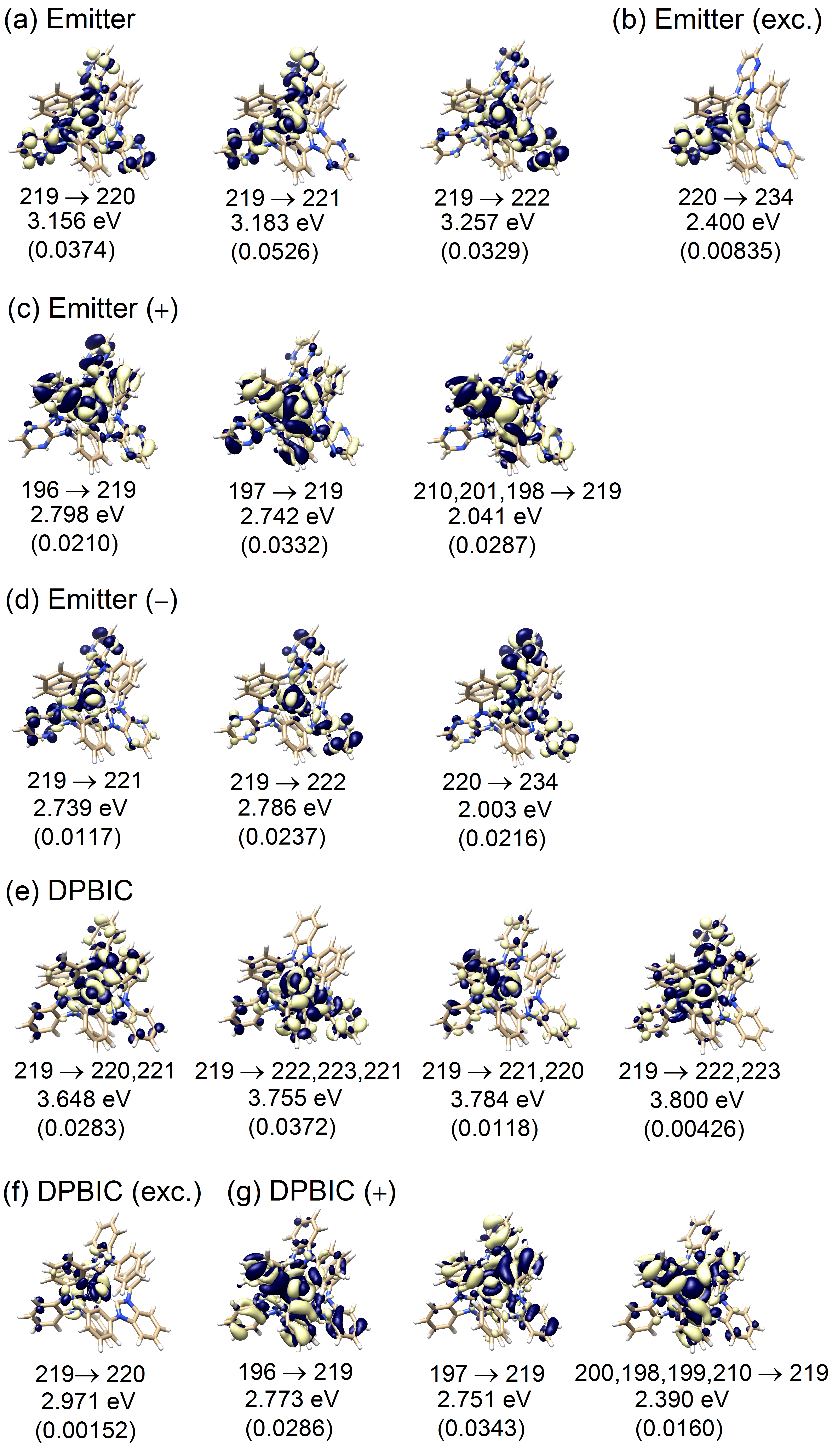
Figure 3: Contour plots of transition densities for (a) ground-state, (b) excited, (c) positively charged and (d) negatively charged NHC blue emitter and (e) ground-state, (f) excited and (g) positively charged DPBIC. For the neutral species, the lowest-energy transitions are shown. For the charged species, bright excitations close to the emission peak of the NHC dye are included. Isosurfaces correspond to 0.0003 Å^-3. The indices of the orbitals taking part in the excitations, excitation energies and oscillator strength (in braces) are shown below the transition densities. Carbon, nitrogen, hydrogen and iridium atoms are coloured in beige, blue, white and sea blue, respectively. The transition densities are obtained by solving the Casida equation without account of spin-orbit coupling for isolated complexes using the PBE0 functional, def2-TZVP basis sets and def2/J auxiliary basis sets.

The absorption spectra for the emitter and DPBIC computed without account of spin-orbit coupling are shown in Figs. 4b and e, respectively. It should be noted that when spectral broadening is taken into account, the calculated absorption spectrum for DPBIC shows a good agreement with the experimental data Haneder (2009) (Fig. 2).

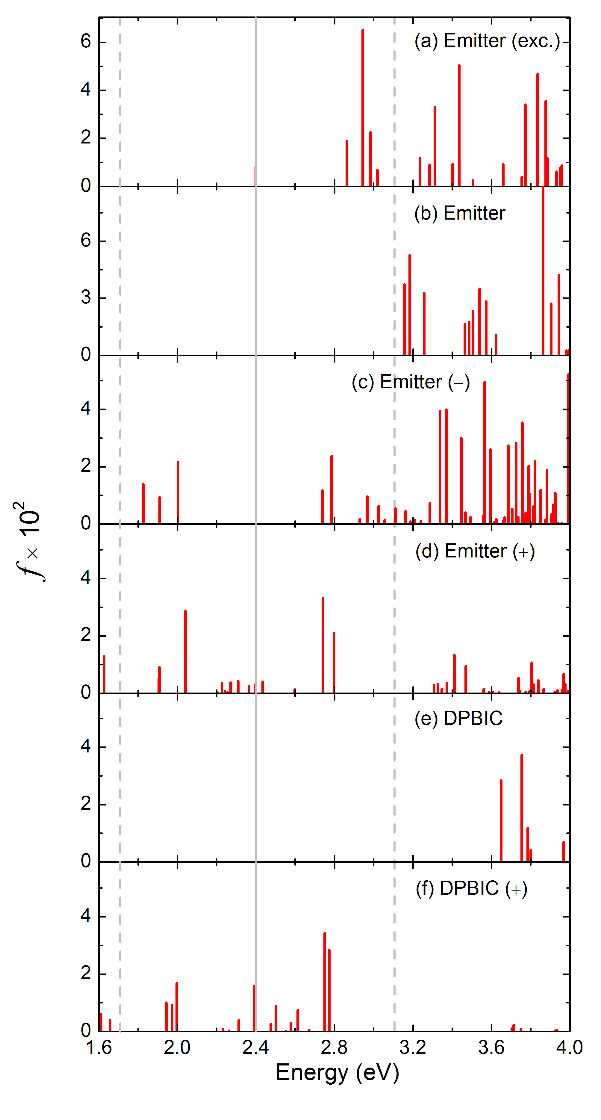
Figure 4: Computed oscillator strengths $f$ of optical transitions at different energies (in eV) for the following species: (a) NHC blue emitter in the excited-state geometry, (b) NHC blue emitter in the ground-state geometry, (c) negatively charged NHC blue emitter, (d) positively charged NHC blue emitter, (e) DPBIC in the ground-state geometry and (f) positively charged DPBIC. The energy corresponding to the emission of the NHC blue emitter of 2.4 eV is indicated by the vertical grey line. The energy interval $2.4\pm 0.7$ eV, where the optical transitions in the charged species significantly contribute to the exciton transfer, is shown by the vertical dashed lines. The spectra are obtained by solving the Casida equation without account of spin-orbit coupling for isolated complexes using the PBE0 functional, def2-TZVP basis sets and def2/J auxiliary basis sets.

III.2 Neutral species in excited-state geometry

Geometry optimization of the first excited states of the NHC blue emitter and DPBIC leads to the decrease of the excitation energy by 0.76 eV and 0.68 eV, respectively. Note that these reorganization energies are larger than typical values found for iridium complexes of 0.2 – 0.5 eV de Vries et al. (2019). The two contributions to the reorganization energy, $\lambda_{ex}$ and $\lambda_{gr}$, related to the structural rearrangements of the acceptor and donor are listed in Table 1.

The calculated energy at which fluorescence takes place for DPBIC of about 3.0 eV agrees well with the positions of the maximum at 3.0 eV Haneder et al. (2008) and 3.2 eV Erk et al. (2006) in the experimentally measured photoluminescence spectra (Fig. 2) and the optical band gap of 3.2 eV determined experimentally in Ref. Haneder et al., 2008. Note that the singlet-triplet splitting in this material is small because of the strong spin-orbit coupling. This was shown in ab initio calculations Haneder (2009); Haneder et al. (2008) and is consistent with the experimentally measured small radiative lifetimes Haneder (2009). Therefore, fluorescence and phosphorescence frequencies of DPBIC should be almost the same. The calculated energy at which fluorescence takes place for the NHC blue emitter of 2.4 eV is also in agreement with the position of the peak maximum in the corresponding electroluminescence spectrum at 2.6 eVNiu et al. (2017).

Table 1: Reorganization energies, $\lambda$, and contributions to the reorganization energy from the geometry relaxation of the excited state, $\lambda_{\mathrm{ex}}$, and ground state, $\lambda_{\mathrm{gr}}$, computed for the NHC blue emitter and DPBIC.

Complex	$\lambda$ (eV)	$\lambda_{\mathrm{ex}}$ (eV)	$\lambda_{\mathrm{gr}}$ (eV)
Blue emitter	0.756	0.3789	0.3776
DPBIC	0.677	0.2263	0.4506

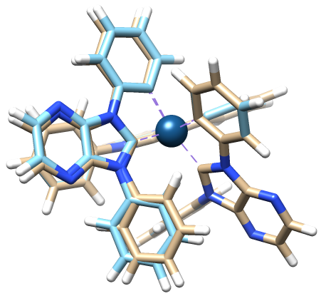
Figure 5: Atomic structures of the optimized ground and excited-state geometries of the NHC blue emitter. Carbon atoms in the ground and excited-state geometries are shown in beige and cyan, respectively. Nitrogen, hydrogen and iridium atoms are coloured in blue, white and sea blue, respectively. The positions of two ligands and the metal atom are the same in the ground and excited-state geometries. The Casida equation is solved without account of spin-orbit coupling for the isolated complexes using the PBE0 functional, def2-TZVP basis sets and def2/J auxiliary basis sets.

In the excited-state geometry, LUMOs of both of the organometallic complexes considered are no longer degenerate and HOMOs are not symmetric (Figs. S2b and f in Supplementary Information). HOMOs are mostly localized on the A fragment of one of the ligands and the metal atom. In the NHC blue emitter, LUMO is centered on the B fragment of the same ligand, while LUMO of DPBIC occupies the C fragment of another ligand that is close to the A fragment carrying HOMO. The first optical transition of both of the complexes in the excited state geometry, therefore, has a metal-ligand charge transfer (MLCT) character (Figs. 3b and f). For DPBIC, where the MLCT character is particularly pronounced, this conclusion is supported by the poorly resolved vibronic structure of the emission spectrum Haneder (2009); Haneder et al. (2008) (see also Fig. 2). A consequence of the strong MLCT character of the first optical transition is that reorganization of the complex geometry upon the excitation is accompanied by a significant decrease in the transition dipole moment and oscillator strength. For the NHC blue emitter, there is a two-fold reduction in the transition dipole moment and more than a four-fold drop in the oscillator strength (Figs. 3a, d and 4a, b). For DPBIC, the changes in the transition dipole moment and oscillator strength of the first optical transition are even more dramatic. The transition dipole moment decreases by a factor of 4 and the oscillator strength almost by a factor of 20 (Figs. 3a and c).

It should be mentioned that for the NHC blue emitter, the geometry relaxation induced by the excitation is mostly related to structural reconstruction of only one ligand (Fig. 5). When two other ligands, the metal atom and dihedral angles within the optimized ligand are fixed during the geometry optimization of the excited state starting from the ground-state geometry, the reorganization energy of the emitter complex decreases only by 0.07 eV. This can be attributed to the localization of HOMO and LUMO on the same ligand of the NHC blue emitter. For DPBIC, two ligands are involved in the geometry relaxation upon the excitation in accordance with the distribution of HOMO and LUMO (Fig. S2f in Supplementary Information).

As seen from the absorption spectra shown in Figs. 4a and e, there is a large energy gap (1.25 eV) between the emission of the NHC blue emitter, which happens at the energy of the first absorption peak in the excited-state geometry, and absorption edge of DPBIC. Therefore, the transfer of excitons from the emitter complex to DPBIC is unlikely. The significant difference in the positions of the absorption edge and emission peak of the NHC blue emitter (Figs. 4a and b) can also lead to suppression of the exciton transport between emitter complexes.

III.3 Charged species

Let us now discuss whether the exciton transfer is possible to charged complexes within the emission layer, i.e. to negatively and positively charged NHC blue emitter and positively charged DPBIC. The absorption spectra of these species in the ground-state geometry are shown in Figs. 4c, d and f and all of them have an overlap with the first absorption peak of the neutral NHC emitter in the excited-state geometry responsible for emission.

We assume that the reorganization energy for the charged complexes is the same as for the neutral ones (in fact our calculations of the transfer rates reveal that they are insensitive to the reorganization energies used for charged species). Therefore, the most relevant optical transitions of the charged species we should analyze lie in the interval of excitation energies of $2.4\pm 0.7$ eV centered at the emission peak of the neutral NHC blue emitter (Figs. 4, 3b,c).

In the negatively charged blue emitter, one of the LUMOs of the emitter gets occupied. HOMO, LUMO+1 and LUMO+2, however, still resemble those in the neutral complex and the transitions between them result to be within the energy interval of interest (peaks at 2.73 eV and 2.79 eV in Fig. 3d). The contribution of these optical transitions to the exciton transfer is expectable. At low excitation energies within the considered energy interval (Fig. 4c), there are also optical transitions that are not present in the neutral complex: from LUMO to high-energy states (Fig. 3d). The oscillator strengths of these transitions are comparable to the transitions HOMO$\to$LUMO+1 and HOMO$\to$LUMO+2.

In the positively charged blue emitter, the optical transitions within the energy interval of interest are related to transitions from low-lying states to the lowest unoccupied state coming from HOMO of the neutral complex (Fig. 3c). The oscillator strengths of some of these transitions (like between molecular orbitals 196$\to$219 and 197$\to$219) are on the order of those for the relevant optical transitions in the negatively charged blue emitter. However, in addition, there are plenty of optical transitions with smaller oscillator strengths close in energy to the emission peak of the NHC blue emitter (Fig. 4d). In spite of the reduced oscillator strengths, it can be expected that such transitions contribute remarkably to the exciton transfer because of the smaller energy shift.

Similar observations can be also done for optical transitions in positively charged DPBIC (Figs. 3g and 4f). A bright example is that similarities in molecular orbitals 196, 197 and 219 (HOMO of neutral species) of the NHC blue emitter and DPBIC provide very close frequencies, oscillator strengths and transition densities for optical transitions 196$\to$219 and 197$\to$219 in these two complexes (Figs. 3d and g). The same as in the positively charged blue emitter, in positively charged DPBIC, there are also a number of optical transitions with comparable or smaller oscillator strengths close in energy to the emission peak of the NHC blue emitter (Fig. 4f).

IV Triplet spectra

The absorption spectra of the NHC blue emitter in the ground and excited-state geometries obtained with account of spin-orbit coupling are shown in Figs. 6a and b, respectively. These spectra have been computed using the Sternheimer approach and LDA functional. For comparison, we also show the spectra obtained with the same approach but without account of spin-orbit coupling (the corresponding peaks are marked here and below as $S_{m}^{0}$, where $m$ is the peak index). Since the LDA functional is known to strongly underestimate the band gap, we apply the scissor operator, i.e. rigidly shift the spectra to higher energies changing the cross-section proportional to energy (that is keeping the values of transition dipole moments, see Eqs. (25) and (29)). The blue shift of 0.95 eV is used for the ground-state geometry and 0.86 eV for the excited-state one to reproduce positions of the first peaks from the PBE0 calculations without account of spin-orbit coupling (Figs. 4a,b and Fig. 6).

From Fig. 6, it follows that the energy difference between the first peaks corresponding to singlet and triplet excitons is about 0.10 eV and 0.06 eV for the ground and excited-state geometries, respectively. Therefore, our results confirm that the the singlet-triplet splitting is very small for the NHC blue emitter. The amplitudes of the highest triplet peaks (T₂, T₆ and T₇ for the ground-state geometry and T^∗ for the excited state one) are an order of magnitude smaller than those of the first singlet peaks. Thus, it can be expected that transport phenomena involving triplet excitons occur slower compared to those for singlet excitons.

From comparison of the data obtained with and without account of spin-orbit coupling in Fig. 6, it is seen that account of spin-orbit coupling leads to changes in the peaks corresponding to singlet excitons. A small red shift of these peaks by 0.05–0.06 eV is observed. Additionally, their amplitudes are increased by 30% and 60% for the ground and excited-state geometries, respectively.

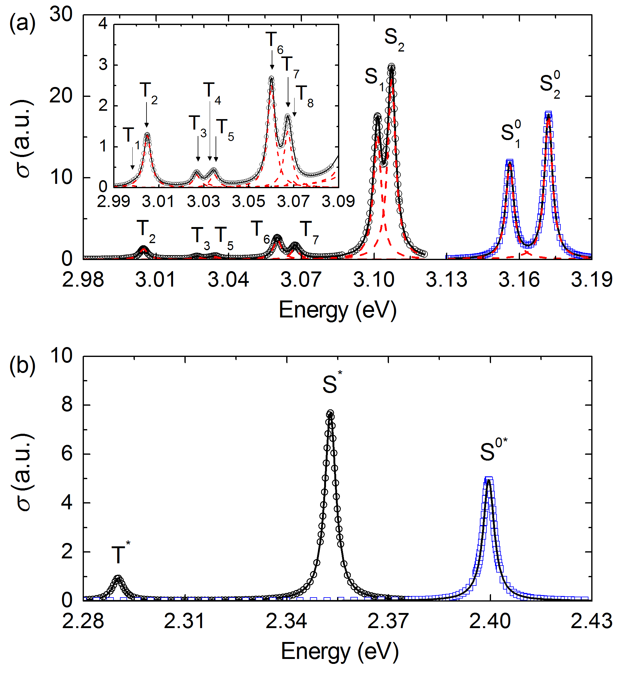
Figure 6: Absorption cross-sections (in a. u.) of the NHC blue emitter in the ground-state (a) and excited-state (b) geometries computed with (black circles) and without (blue squares) account of spin-orbit coupling. The insert in panel (a) shows the part of the spectrum corresponding to triplet excitons with a higher resolution. Approximations by sums of Lorentzian functions are shown by black solid lines. Contributions of individual Lorentzian functions are indicated by red dashed lines. The peaks corresponding to singlet and triplet excitons are denoted by letters S and T, respectively, and are numbered consecutively. The peaks for the excited-state geometry are marked by an asterisk. The peaks obtained without account of spin-orbit coupling are denoted as S⁰. The Sternheimer equation with the linewidth parameter of $\hbar\eta=2$ meV is solved for the isolated complexes using the regular real-space grid with spacing of 0.14 Å and the LDA functional. The scissor operator is applied to correct the band gap.

To extract the transition dipole moments, the spectra are fitted by a sum of Lorentzian functions given by Eq. (38):

$$\sigma(\omega)=\sum_{m=1}^{M}\sigma_{m}f_{0}^{\mathrm{L}}(\omega-\Omega_{m}).$$ (39)

As seen from Eqs. (25) and (29), parameters $\sigma_{m}$ can be expressed through the oscillator strength or transition dipole moment as $\sigma_{m}=2\pi^{2}e^{2}f_{m}/(m_{e}c)=4\pi^{2}\Omega_{m}|\mathbf{d}_{m}^{\mathrm{T}}|^{2}/(3\hbar c)$. The parameters of Eq. 39 that minimize the root-mean-square deviation from the computed data as well as estimated transition dipole moments are given in Table 2.

The transition dipole moment for the emitter in the excited state can be used to estimate the exciton radiative lifetime according to the equation Mori et al. (2014); de Vries et al. (2019); de Vries, Coehoorn, and Bobbert (2020); Strickler and Berg (2004); Nozaki (2006)

$$\frac{1}{\tau_{\mathrm{r,m}}}=\frac{4\epsilon_{\mathrm{r}}\Omega_{m}^{3}|\mathbf{d}_{m}^{\mathrm{T}}|^{2}}{3\hbar c^{3}}.$$ (40)

Here $\epsilon_{\mathrm{r}}$ is the optical dielectric permittivity of the surrounding medium, which typically can be taken equal to $\epsilon_{\mathrm{r}}=3$ for OLED emission layersSalehi et al. (2018); Liu et al. (2005). For triplet excitons (peak T^∗), this gives $\tau_{\mathrm{r,T}}\sim 1$ $\mu$s, within the range of values 0.5 – 10 $\mu$s obtained for other iridium complexes Haneder (2009); Haneder et al. (2008); de Vries et al. (2019); de Vries, Coehoorn, and Bobbert (2020); Ligthart et al. (2021, 2018). For singlet excitons (peak S^∗), the radiative lifetime is estimated to be $\tau_{\mathrm{r,S}}\sim 0.1$ $\mu$s. This is not that small as for fluorescent dyes Giebink and Forrest (2008) because of the relatively low oscillator strength (Table 2).

Table 2: Characteristics of the first optical transitions of the NHC blue emitter in the ground and excited-state geometries obtained by fitting the spectra computed by solving the Sternheimer equation for isolated complexes with and without account of spin-orbit coupling.

Peak	$\hbar\Omega$ (eV)	$\sigma\times 10^{3}$ (a.u.)	$f\times 10^{2}$	$|\mathbf{d}^{\mathrm{T}}|^{2}$ (a.u.2)
Ground-state geometry with spin-orbit coupling
T1	2.999	0.012	0.008	0.001
T2	3.005	0.295	0.204	0.028
T3	3.027	0.073	0.050	0.007
T4	3.032	0.020	0.014	0.002
T5	3.035	0.076	0.053	0.007
T6	3.060	0.578	0.401	0.054
T7	3.067	0.321	0.223	0.030
T8	3.069	0.040	0.028	0.004
S1	3.101	3.524	2.446	0.322
S2	3.107	5.098	3.539	0.465
Excited-state geometry with spin-orbit coupling
T∗	2.290	0.214	0.149	0.027
S∗	2.353	1.775	1.232	0.214
Ground-state geometry without spin-orbit coupling
S${}_{1}^{0}$	3.156	2.694	1.870	0.242
S${}_{2}^{0}$	3.172	4.074	2.827	0.364
Excited-state geometry without spin-orbit coupling
S0∗	2.400	1.143	0.793	0.135

Let us now discuss the accuracy of the LDA calculations. As seen from Table 2, the transition dipole moments for singlet excitons computed using the LDA functional without account of spin-orbit coupling are fairly close to the results of PBE0 calculations. The squares of the transition dipole moments are different by a factor of 2 for the ground-state geometry and by less than 5% for the excited-state one. It should be also noted that the difference in the positions of the absorption edge and emission peak computed with the LDA functional without account of spin-orbit coupling is less than the same quantity for PBE0 only by 0.1 eV. A qualitative similarity in the results of LDA and PBE0 calculations using the same ORCA code can be also appreciated in Fig. S1 of Supplementary Information. Therefore, the LDA functional is sufficient for qualitative studies of exciton dynamics.

V Dexter vs. Förster mechanisms

To consider the contributions of different mechanisms to the exciton coupling, we have performed real-time propagation for a dimer consisting of NHC blue emitters in the ground and excited state geometries. The organometallic complexes are separated by 1.2 nm (the distance between the metal atoms), which is a typical distance between them in the considered emission layer. The total absorption cross-section for the dimer is shown in Fig. 7a. The total spectrum is divided into the donor (emitter in the excited state) and acceptor (emitter in the ground state) contributions using the QTAIM approach Bader (1994). It is seen from Fig. 7a that positions of the emission peak S^0∗ and first absorption peaks of the donor, S${}_{1}^{0}$ and S${}_{2}^{0}$, are rather close to those obtained using the Sternheimer equation for the isolated emitters in the excited and ground states, respectively (Fig. 6b, Table 2).

By diagonalization of the cross-section tensors for the donor and acceptor at each frequency, we extract the cross-section eigenvalues and approximate them by the sum of Gaussian functions (Figs. 7b and c). For the considered propagation time and damping applied to the spectra, $\mathrm{HWHM}$ is 0.016 eV. The fitted parameters and estimated transition dipole moments are listed in Table 3. As seen from comparison with Table 2, the transition dipole moments obtained by the real-time propagation are about 10% less than the values from the Sternheimer equation. This decrease can be attributed to the effect of the interaction between the donor and acceptor complexes taken into account explicitly in the real-time propagation Jornet-Somoza and Lebedeva (2019).

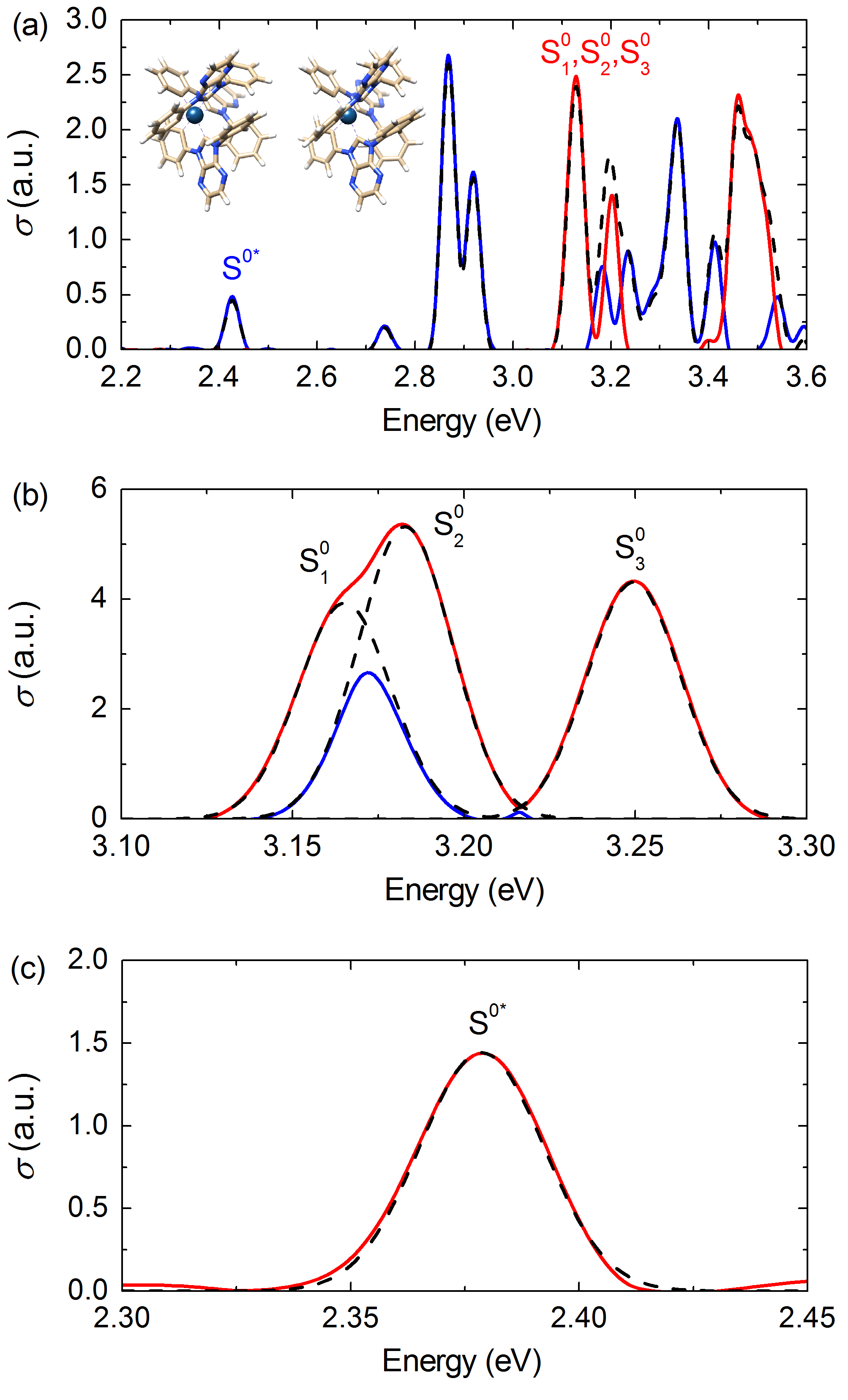
Figure 7: (a) Absorption cross-section (in a. u.) of the dimer consisting of the NHC blue emitters in the ground (acceptor) and excited (donor) states. The acceptor (red solid line), donor (blue solid line) and total (black dashed line) contributions are shown. The insert demonstrates the atomic structure of the dimer. (b) The largest (red solid line) and the medium (blue solid line) eigenvalues of the cross-section tensor for the acceptor at the absorption edge. (c) The largest eigenvalue of the cross-section tensor for the donor at the absorption edge. Fitting by individual Gaussian functions is shown in panels (b) and (c) by black dashed lines. The results are obtained by the real-time propagation for the dimer using the regular real-space grid with spacing of 0.14 Å and the LDA functional. The scissor operator is applied to correct the band gap. The spin-orbit coupling is not taken into account.

Table 3: Characteristics of the first optical transitions of the NHC blue emitter in the ground and excited-state geometries obtained by fitting the results of the real-time propagation for the emitter dimer.

Peak	$\hbar\Omega$ (eV)	$\sigma\times 10^{3}$ (a.u.)	$f\times 10^{2}$	$|\mathbf{d}^{\mathrm{T}}|^{2}$ (a.u.2)	$e_{x}$	$e_{y}$	$e_{z}$
Ground-state geometry
S${}_{1}^{0}$	3.165	2.346	1.628	0.210	-0.267	0.314	0.911
S${}_{2}^{0}$	3.183	3.168	2.199	0.282	-0.170	-0.554	0.815
S${}_{3}^{0}$	3.250	2.546	1.177	0.222	-0.449	-0.642	-0.621
Excited-state geometry
S0∗	2.380	0.941	0.653	0.112	0.144	-0.9847	0.065

After evaluation of the transition dipole moments, the fast Fourier transform of the response electron density is performed at frequencies corresponding to peaks S^0∗, S${}_{1}^{0}$, S${}_{2}^{0}$ and S${}_{3}^{0}$ and the Fourier-transformed densities are divided into the contributions corresponding to the donor and acceptor. Using the transition dipole moments from Table 3 (including their directions $\mathbf{e}$), we find the transition densities for the donor at peak S^0∗ and for the acceptor at peaks S${}_{1}^{0}$, S${}_{2}^{0}$ and S${}_{3}^{0}$ according to Eq. (23). The Förster and Dexter exciton couplings computed using the explicit integration over the transition densities (TCDM approach) as well as the IDA Förster coupling evaluated according to Eqs. (5), (16) and (8) are listed in Table 4.

It is seen from Table 4 that the Förster couplings computed taking into account spatial distributions of the transition densities given by Eq. (5) lie in the same range of magnitudes as the IDA results. Nevertheless, the values for the same peak differ considerably. This is in agreement with results of our previous paper Jornet-Somoza and Lebedeva (2019) that IDA is adequate for distances well above 1.2 nm.

The Dexter coupling is several orders of magnitude smaller than the coupling for the Förster mechanism (Table 4). It is completely zero for LDA Perdew and Zunger (1981) since in this approximation, the exchange-correlation effects are completely local. The generalized gradient approximation like PBE Perdew, Burke, and Ernzerhof (1996) gives the Dexter coupling 3 – 5 orders of magnitude smaller than the Förster one. The PBE0 Adamo and Barone (1999) and HSE06 Heyd, Scuseria, and Ernzerhof (2003); Krukau et al. (2006) functionals taking into account a fraction of the exact exchange provide similar results, although another hybrid functional B3LYP Lu et al. (2013) predicts an increase in the Dexter coupling by an order of magnitude. In general, however, it can be concluded that for distances 1.2 nm and more, typical for the OLED emission layer, the Dexter coupling can be neglected in comparison with the Förster coupling. Note that kinetic Monte-Carlo simulations Mesta et al. (2016) support that roll-off of white OLEDs occurs via long-range Förster mechanism rather than by short-range nearest-neighbour quenching. In the following, we limit our consideration to the Förster mechanism.

Table 4: Förster ($V_{\mathrm{F}}$) and Dexter ($V_{\mathrm{D}}$) coupling and coupling in the ideal dipole approximation ($V_{\mathrm{F}}^{\mathrm{IDA}}$) computed for exciton transfer from the lowest excited state of the excited emitter ($\hbar\Omega_{\mathrm{D}}=2.380$ eV) to the lowest excited states of the emitter in the ground state from the results of real-time propagation for the emitter dimer .

Peak	$\hbar\Omega$	$V_{\mathrm{F}}$	$V_{\mathrm{D}}$ (meV)					$V_{\mathrm{F}}^{\mathrm{IDA}}$
	(meV)	(meV)	LDA	PBE	PBE0	HSE06	B3LYP	(meV)
S${}^{0}_{1}$	3.165	0.494	0	$1.03\cdot 10^{-4}$	$8.31\cdot 10^{-5}$	$1.29\cdot 10^{-4}$	$1.40\cdot 10^{-3}$	0.061
S${}^{0}_{2}$	3.183	0.570	0	$4.62\cdot 10^{-5}$	$4.00\cdot 10^{-5}$	$1.78\cdot 10^{-5}$	$8.57\cdot 10^{-4}$	0.269
S${}^{0}_{3}$	3.250	0.042	0	$7.73\cdot 10^{-5}$	$4.84\cdot 10^{-5}$	$7.41\cdot 10^{-5}$	$2.22\cdot 10^{-2}$	0.268

VI Transfer rates

VI.1 Singlet excitons

Although the IDA (Eq. (8)) fails to describe the exciton coupling between nearest neighbours, it still gives the correct order of magnitude and becomes quantitatively correct at large distances. Therefore, here we use the IDA for qualitative analysis of transfer rates to different species in the emission layer. To take into account the effect of the surrounding dielectric medium, we multiply the exciton coupling in vacuum (Eq. 8) by the screening factor $V_{\mathrm{DA}}=sV_{\mathrm{F}}^{\mathrm{IDA}}$. As discussed in previous papers Mennucci and Curutchet (2011); Harriman and Ziessel (2010); Juzeliūnas and Andrews (1994), the environmental effects can be divided into two contributions $s=f_{s}^{2}\cdot 1/\epsilon_{\mathrm{r}}$, changes in effective dipole strengths, $f_{s}$, and Coulomb screening, $1/\epsilon_{\mathrm{r}}$. For the first term, the Onsager expression for empty cavity Aubret, Orrit, and Kulzer (2019) is often usedMennucci and Curutchet (2011), $f_{s}=3\epsilon_{\mathrm{r}}/(2\epsilon_{\mathrm{r}}+1)$. This gives $s\sim 0.55$ for the medium with typical $\epsilon_{\mathrm{r}}=3$. For simplicity, we also take the orientational factor $\kappa^{\mathrm{DA}}$ in Eq. (8) equal to unity.

The estimates of exciton transfer rates between NHC iridium complexes obtained using the Marcus and Levich-Jortner expressions (Eqs. 26 and 27, respectively) are presented in Table 5 (the transition dipole moments used in the calculation can be found in Supplementary Information). The values computed with the Marcus and Levich-Jortner expressions are similar qualitatively and in many cases even quantitatively. The data also confirm the qualitative conclusions drawn before through the analysis of the absorption spectra (Fig. 4).

As expected, because of the huge shift between the emission spectrum of the NHC blue emitter and absorption spectrum of neutral DPBIC, the rate of exciton transfer to DPBIC is negligibly small compared to the transfer to the NHC blue emitter (Table 5). Although the exact value of this rate is sensitive to the model employed, it is vanishing for both of the models considered.

There is also a significant energy shift between the emission peak and absorption edge of the NHC blue emitter itself. Furthermore, the oscillator strengths of the first optical transitions are rather small and the intermolecular distances between the organometallic complexes are relatively large (exceed 1 nm even for the nearest neighbours) providing small exciton couplings for pairs of emitter complexes as well. As a result, the transfer of excitons between two emitter complexes is also slow (Table 5). Although the rate increases twice when the Levich-Jortner model is used instead of the Marcus one, the characteristic transfer time in any case is comparable with the previously estimated singlet radiative lifetime ($\tau_{\mathrm{r,S}}\sim$ 0.1 $\mu$s, see Eq. 40).

The Förster exciton transfer is often characterized using the effective Förster radius $R^{\mathrm{F}}$ (Refs. van Eersel et al., 2014, 2016; Mesta et al., 2016; Coehoorn, Bobbert, and van Eersel, 2017; de Vries et al., 2019; de Vries, Coehoorn, and Bobbert, 2020; Ligthart et al., 2021)

$$k(R)=\frac{1}{\tau_{\mathrm{r}}}\left(\frac{R^{\mathrm{F}}}{R}\right)^{6},$$ (41)

where $k$ is the transfer rate and $R$ is the distance between the donor and acceptor. Using $\tau_{\mathrm{r,S}}\sim$ 0.1 $\mu$s, we estimate the Förster radius for singlet diffusion to be $R^{\mathrm{F}}_{\mathrm{diff,S}}\sim$ 1 nm. This means that singlet diffusion is basically suppressed. At most some excitons can be transferred once to a nearest neighbour blue emitter before the decay.

The rates of exciton transfer to the charged species are two-three orders of magnitude greater compared to the transfer to the neutral NHC blue emitter (Table 5) due to the significant overlap between the absorption spectra of the charged species with the emission peak of the blue emitter. As can be estimated from the equation similar to Eq. 41, the Förster radius for exciton-polaron quenching is $R^{\mathrm{F}}_{\mathrm{e,S}}\sim$ 2.4 nm for electrones and $R^{\mathrm{F}}_{\mathrm{h,S}}\sim$ 2.7 nm for holes. The exciton quenching should thus occur with a large probability if an electron or a hole gets within this distance from the exciton.

Integrating the exciton transfer rate for distances greater than some minimal distance $R_{\mathrm{min}}$, the characteristic rates of exciton-polaron quenching can be estimated as

$$k_{\mathrm{p}}=k_{0}\left(R^{\mathrm{F}}_{\mathrm{p}}\right)^{6}\int_{R_{\mathrm{min}}}^{\infty}\frac{4\pi R^{2}dR}{R^{6}}=\frac{4\pi k_{0}\left(R^{\mathrm{F}}_{\mathrm{p}}\right)^{6}}{3R_{\mathrm{min}}^{3}},$$ (42)

where $R^{\mathrm{F}}_{\mathrm{p}}$ is the Förster radius for exciton-polaron quenching. Using $R_{\mathrm{min}}\sim 1$ nm, which corresponds to the minimal distance between organometallic complexes in the considered emission layer, we obtain $k_{\mathrm{h,S}}\sim 2\cdot 10^{-11}$ cm${}^{3}/$s for holes and $k_{\mathrm{e,S}}\sim 8\cdot 10^{-12}$ cm${}^{3}/$s for electrons. As seen from these results, the transfer rates to the positively charged species are greater than for the negatively charged emitter implying that in the considered OLED, holes are more efficient in exciton quenching as compared to electrons.

It should be noted that the transfer rates to the positively charged emitter and DPBIC are comparable and are not sensitive to the model employed. The latter is explained by the fact that the transfer is dominated by the optical transitions relatively close to the emission peak of the NHC blue emitter. For positively charged DPBIC, the largest contribution to the transfer rate corresponds to the peak at 2.4 eV, while for the positively charged blue emitter, several peaks in the range from 2.0 eV to 2.6 eV contribute in a similar way. The transfer rate to the negatively charged emitter, on the other hand, increases by a factor of 1.5 when the Levich-Jortner expression is used because of the dominant contribution from the optical transitions far from the emission peak of the NHC blue emitter. The most intensive transfer occurs here to the peak at 2.0 eV. We have checked that the estimated exciton transfer rates to charged species weakly depend on their contributions to the reorganization energies used for them if they lie in the range of 0 – 0.5 eV.

Table 5: Rates of exciton transfer from the excited NHC blue emitter (characterized by $\hbar\Omega_{\mathrm{D}}=2.400$ eV and $|\mathbf{d}_{\mathrm{D}}^{\mathrm{T}}|^{2}=0.1420$ a.u.²) to different species of the emission layer computed at temperature $T=$300 K for the nearest-neighbour intermolecular distance of $R=1$ nm.

Acceptor	$\hbar\Omega_{\mathrm{A}}$	$|\mathbf{d}_{\mathrm{A}}^{\mathrm{T}}|^{2}$	$V_{\mathrm{DA}}$	$\Delta$	$J_{\mathrm{M}}$	$k_{\mathrm{M}}$	$k_{\mathrm{M,tot}}$	$J_{\mathrm{LH}}$	$k_{\mathrm{LH}}$	$k_{\mathrm{LH,tot}}$
	(eV)	(a.u.2)	(meV)	(eV)	(eV-1)	(s-1)	(s-1)	(eV-1)	(s-1)	(s-1)
Blue emitter	3.156	0.484	0.581	0.757	$1.3\cdot 10^{-3}$	$4.3\cdot 10^{6}$	$5.6\cdot 10^{6}$	$2.7\cdot 10^{-3}$	$8.8\cdot 10^{6}$	$1.1\cdot 10^{7}$
(neutr.)	3.183	0.675	0.687	0.783	$7.9\cdot 10^{-4}$	$3.6\cdot 10^{6}$		$1.6\cdot 10^{-3}$	$7.2\cdot 10^{6}$
	3.257	0.412	0.537	0.858	$1.7\cdot 10^{-4}$	$4.6\cdot 10^{5}$		$3.2\cdot 10^{-4}$	$8.6\cdot 10^{5}$
Blue emitter ($-$)	1.825	0.314	0.468	-0.574	$3.0\cdot 10^{-2}$	$6.2\cdot 10^{7}$	$1.2\cdot 10^{9}$	$1.2\cdot 10^{-1}$	$2.4\cdot 10^{8}$	$1.8\cdot 10^{9}$
	1.910	0.197	0.371	-0.490	$9.4\cdot 10^{-2}$	$1.2\cdot 10^{8}$		$2.2\cdot 10^{-1}$	$2.9\cdot 10^{8}$
	2.003	0.441	0.555	-0.396	$2.7\cdot 10^{-1}$	$8.0\cdot 10^{8}$		$4.0\cdot 10^{-1}$	$1.2\cdot 10^{9}$
	2.739	0.174	0.349	0.340	$4.6\cdot 10^{-1}$	$5.4\cdot 10^{8}$		$6.3\cdot 10^{-1}$	$7.4\cdot 10^{8}$
	2.786	0.347	0.492	0.386	$3.0\cdot 10^{-1}$	$6.9\cdot 10^{8}$		$4.5\cdot 10^{-1}$	$1.0\cdot 10^{9}$
Blue emitter (+)	2.041	0.573	0.633	-0.359	$3.9\cdot 10^{-1}$	$1.5\cdot 10^{9}$	$2.9\cdot 10^{9}$	$5.0\cdot 10^{-1}$	$1.9\cdot 10^{9}$	$3.3\cdot 10^{9}$
	2.227	0.064	0.212	-0.172	1.4	$5.9\cdot 10^{8}$		1.2	$5.1\cdot 10^{8}$
	2.272	0.067	0.217	-0.127	1.6	$7.3\cdot 10^{8}$		1.4	$6.1\cdot 10^{8}$
	2.309	0.075	0.230	-0.090	1.8	$9.1\cdot 10^{8}$		1.5	$7.5\cdot 10^{8}$
	2.365	0.042	0.171	-0.034	2.0	$5.6\cdot 10^{8}$		1.6	$4.6\cdot 10^{8}$
	2.398	0.054	0.195	-0.002	2.0	$7.3\cdot 10^{8}$		1.7	$6.1\cdot 10^{8}$
	2.435	0.068	0.218	0.035	2.0	$9.0\cdot 10^{8}$		1.7	$7.8\cdot 10^{8}$
	2.742	0.494	0.587	0.342	$4.5\cdot 10^{-1}$	$1.5\cdot 10^{9}$		$6.2\cdot 10^{-1}$	$2.1\cdot 10^{9}$
	2.798	0.307	0.463	0.399	$2.6\cdot 10^{-1}$	$5.4\cdot 10^{8}$		$4.0\cdot 10^{-1}$	$8.2\cdot 10^{8}$
DPBIC	3.648	0.317	0.471	1.249	$3.2\cdot 10^{-11}$	$6.8\cdot 10^{-2}$	$6.8\cdot 10^{-2}$	$2.3\cdot 10^{-12}$	$4.9\cdot 10^{-3}$	$4.9\cdot 10^{-3}$
(neutr.)	3.755	0.405	0.532	1.355	$3.8\cdot 10^{-13}$	$1.0\cdot 10^{-3}$		$8.3\cdot 10^{-15}$	$2.2\cdot 10^{-5}$
	3.784	0.128	0.299	1.385	$1.0\cdot 10^{-13}$	$8.8\cdot 10^{-5}$		$1.6\cdot 10^{-15}$	$1.3\cdot 10^{-6}$
	3.800	0.049	0.179	1.401	$5.1\cdot 10^{-14}$	$1.6\cdot 10^{-5}$		$6.3\cdot 10^{-16}$	$1.9\cdot 10^{-7}$
DPBIC (+)	1.997	0.342	0.489	-0.403	$1.7\cdot 10^{-1}$	$3.8\cdot 10^{8}$	$4.9\cdot 10^{9}$	$3.4\cdot 10^{-1}$	$7.8\cdot 10^{8}$	$4.6\cdot 10^{9}$
	2.313	0.069	0.219	-0.087	2.0	$9.1\cdot 10^{8}$		1.6	$7.1\cdot 10^{8}$
	2.390	0.273	0.437	-0.010	2.3	$4.1\cdot 10^{9}$		1.8	$3.3\cdot 10^{9}$
	2.475	0.045	0.178	0.076	2.1	$6.2\cdot 10^{8}$		1.8	$5.5\cdot 10^{8}$
	2.501	0.143	0.316	0.102	1.9	$1.8\cdot 10^{9}$		1.8	$1.7\cdot 10^{9}$
	2.578	0.046	0.179	0.178	1.4	$4.2\cdot 10^{8}$		1.5	$4.5\cdot 10^{8}$
	2.614	0.118	0.287	0.214	1.1	$8.5\cdot 10^{8}$		1.3	$1.0\cdot 10^{9}$
	2.751	0.508	0.596	0.352	$3.1\cdot 10^{-1}$	$1.1\cdot 10^{9}$		$5.1\cdot 10^{-1}$	$1.7\cdot 10^{8}$
	2.773	0.420	0.542	0.374	$2.4\cdot 10^{-1}$	$6.8\cdot 10^{8}$		$4.1\cdot 10^{-1}$	$1.2\cdot 10^{8}$

VI.2 Triplet excitons

The exciton transfer rates between emitter complexes have been also estimated with account of spin-orbit coupling based on the spectra computed using the Sternheimer equation (Fig. 6, Table 2). The rates of transfer processes in which the donor loses a singlet or triplet exciton and the acceptor acquires a singlet or a triplet exciton are presented in Table 6. A three-fold increase in the singlet transfer rates (S$\to$S) as compared to the calculations without account of spin-orbit coupling (S${}_{0}\to$S₀) is related to the increase in the transition dipole moments.

It is seen from Table 6 that when the acceptor is excited to the triplet state, the transfer rates are only 2–3 times smaller compared to the case when when the acceptor stays singlet (T$\to$T and S$\to$T versus T$\to$S and S$\to$S, respectively). Although the oscillator strengths of the triplet peaks of the emitter in the ground-state geometry are considerably smaller than those of the singlet peaks (Table 2), they are located at lower frequencies and, therefore, the energy shift with respect to the emission peaks of the donor is smaller. For this reason, the contribution of the processes with the triplet exciton on the acceptor is comparable to those with the singlet exciton on the acceptor.

The transfer rates for the initially triplet exciton, on the other hand, are about 30 times smaller than for the singlet exciton (T$\to$T and T$\to$S versus S$\to$T and S$\to$S, respectively). This is because the oscillator strength of the T^∗ peak corresponding to the triplet exciton for the emitter in the excited-state geometry is an order of magnitude smaller compared to the peak S^∗ corresponding to the singlet exciton (Table 2) and the energy shift between the absorption and emission is greater for the T^∗ peak. Therefore, transport of triplet excitons is significantly slower than that of singlet excitons. Using the triplet radiative lifetime $\tau_{\mathrm{r,T}}\sim$ 1 $\mu$s (see Eq. 40), the Förster radius estimated for triplet excitons according to Eq. 41 is $R^{\mathrm{F}}_{\mathrm{diff,S}}\sim$ 0.9 nm, even smaller than for singlet excitons. This value is at the lower bound of the range 1 – 4 nm computed from first principles for diverse iridium-based complexes de Vries et al. (2019); de Vries, Coehoorn, and Bobbert (2020) and shows that exciton diffusion in the considered emission layer is hardly possible.

The estimated rates of singlet and triplet exciton transfer to charged species in the emission layer are listed in Table 7. It is seen that the transfer rates of triplet excitons to the positively charged NHC blue emitter and DPBIC are an order of magnitude smaller than the similar rates for singlet excitons. This is because of the ratio of the transition dipole moments for singlet and triplet excitons. The difference in the transfer rates of triplet and singlet excitons to the negatively charged emitter is smaller. Here the transfer is dominated by the absorption peak of the negatively charged emitter at 2.0 eV that is located closer in energy to the phosphorescence peak of the neutral emitter than to the fluorescence one.

Similar to singlet excitons, the rates of transfer of triplet excitons to charged species are three orders of magnitude higher than to the neutral emitter (Table 7). The Förster radius for triplet-polaron quenching is $R^{\mathrm{F}}_{\mathrm{e,T}}\sim$ 2.8 nm for electrons and $R^{\mathrm{F}}_{\mathrm{h,T}}\sim$ 3.0 nm for holes, close to typical values considered in kinetic Monte Carlo simulations Coehoorn, Bobbert, and van Eersel (2017); Ligthart et al. (2021); Mesta et al. (2016); van Eersel et al. (2014, 2016). The characteristic rates of triplet-polaron quenching are $k_{\mathrm{h,T}}\sim 3\cdot 10^{-12}$ cm${}^{3}/$s for holes and $k_{\mathrm{e,T}}\sim 2\cdot 10^{-12}$ cm${}^{3}/$s for electrons. Note that exciton-polaron quenching rates of $10^{-12}-3\cdot 10^{-11}$ cm${}^{3}/$s were measured for OLEDs with iridium complexes Reineke, Walzer, and Leo (2007); Zhang, Lee, and Forrest (2014); Wehrmeister et al. (2015); Erickson and Holmes (2014); Lee et al. (2016); Hershey and Holmes (2016) and various organic semiconductors Murawski, Leo, and Gather (2013); Zhang et al. (2010).

Table 6: Rates of exciton transfer from the excited NHC blue emitter to the neutral emitter in the ground state estimated for singlet (S) and triplet (T) excitons at temperature $T=$ 300 K for the nearest-neighbour intermolecular distance of $R=1$ nm.

Transfer		$V_{\mathrm{DA}}$	$\Delta$	$J_{\mathrm{M}}$	$k_{\mathrm{M}}$	$k_{\mathrm{M,tot}}$	$J_{\mathrm{LH}}$	$k_{\mathrm{LH}}$	$k_{\mathrm{LH,tot}}$
		(meV)	(eV)	(eV-1)	(s-1)	(s-1)	(eV-1)	(s-1)	(s-1)
T$\to$T	T${}^{*}\to$T1	0.012	0.708	$3.3\cdot 10^{-3}$	$4.6\cdot 10^{3}$	$1.3\cdot 10^{5}$	$6.8\cdot 10^{-3}$	$9.4\cdot 10^{3}$	$2.7\cdot 10^{5}$
	T${}^{*}\to$T2	0.060	0.715	$3.0\cdot 10^{-3}$	$1.0\cdot 10^{5}$		$6.1\cdot 10^{-3}$	$2.1\cdot 10^{5}$
	T${}^{*}\to$T3	0.030	0.737	$2.0\cdot 10^{-3}$	$1.7\cdot 10^{4}$		$4.0\cdot 10^{-3}$	$3.4\cdot 10^{4}$
	T${}^{*}\to$T4	0.016	0.742	$1.8\cdot 10^{-3}$	$4.2\cdot 10^{3}$		$3.6\cdot 10^{-3}$	$8.5\cdot 10^{3}$
	T${}^{*}\to$T5	0.030	0.744	$1.7\cdot 10^{-3}$	$1.5\cdot 10^{4}$		$3.5\cdot 10^{-3}$	$3.1\cdot 10^{4}$
	T${}^{*}\to$T6	0.084	0.770	$1.0\cdot 10^{-3}$	$6.9\cdot 10^{4}$		$2.1\cdot 10^{-3}$	$1.4\cdot 10^{5}$
	T${}^{*}\to$T7	0.062	0.777	$8.9\cdot 10^{-4}$	$3.3\cdot 10^{4}$		$1.8\cdot 10^{-3}$	$6.7\cdot 10^{4}$
	T${}^{*}\to$T8	0.022	0.779	$8.6\cdot 10^{-4}$	$4.0\cdot 10^{3}$		$1.7\cdot 10^{-3}$	$8.1\cdot 10^{3}$
T$\to$S	T${}^{*}\to$S1	0.205	0.811	$4.5\cdot 10^{-4}$	$1.8\cdot 10^{5}$	$2.9\cdot 10^{5}$	$8.9\cdot 10^{-4}$	$3.6\cdot 10^{5}$	$5.8\cdot 10^{5}$
	T${}^{*}\to$S2	0.246	0.817	$4.0\cdot 10^{-4}$	$2.3\cdot 10^{5}$		$7.8\cdot 10^{-4}$	$4.5\cdot 10^{5}$
S$\to$T	S${}^{*}\to$T1	0.034	0.646	$9.8\cdot 10^{-3}$	$1.1\cdot 10^{5}$	$3.2\cdot 10^{6}$	$2.0\cdot 10^{-2}$	$2.2\cdot 10^{5}$	$6.6\cdot 10^{6}$
	S${}^{*}\to$T2	0.171	0.652	$8.8\cdot 10^{-3}$	$2.5\cdot 10^{6}$		$1.8\cdot 10^{-2}$	$5.0\cdot 10^{6}$
	S${}^{*}\to$T3	0.085	0.674	$6.1\cdot 10^{-3}$	$4.1\cdot 10^{5}$		$1.2\cdot 10^{-2}$	$8.5\cdot 10^{5}$
	S${}^{*}\to$T4	0.045	0.679	$5.5\cdot 10^{-3}$	$1.0\cdot 10^{5}$		$1.1\cdot 10^{-2}$	$2.1\cdot 10^{5}$
	S${}^{*}\to$T5	0.086	0.682	$5.3\cdot 10^{-3}$	$3.8\cdot 10^{5}$		$1.1\cdot 10^{-2}$	$7.7\cdot 10^{5}$
	S${}^{*}\to$T6	0.237	0.707	$3.4\cdot 10^{-3}$	$1.8\cdot 10^{6}$		$6.9\cdot 10^{-3}$	$3.7\cdot 10^{6}$
	S${}^{*}\to$T7	0.177	0.715	$3.0\cdot 10^{-3}$	$8.8\cdot 10^{5}$		$6.1\cdot 10^{-3}$	$1.8\cdot 10^{6}$
	S${}^{*}\to$T8	0.063	0.716	$2.9\cdot 10^{-3}$	$1.1\cdot 10^{5}$		$5.9\cdot 10^{-3}$	$2.2\cdot 10^{5}$
S$\to$S	S${}^{*}\to$S1	0.582	0.749	$1.6\cdot 10^{-3}$	$5.0\cdot 10^{6}$	$8.2\cdot 10^{6}$	$3.2\cdot 10^{-3}$	$1.0\cdot 10^{7}$	$1.7\cdot 10^{7}$
	S${}^{*}\to$S2	0.699	0.754	$1.4\cdot 10^{-3}$	$6.5\cdot 10^{6}$		$2.9\cdot 10^{-3}$	$1.3\cdot 10^{7}$
S${}_{0}\to$S0	S${}^{*}_{0}\to$S0,1	0.401	0.757	$1.3\cdot 10^{-3}$	$2.1\cdot 10^{6}$	$3.1\cdot 10^{6}$	$2.7\cdot 10^{-3}$	$4.2\cdot 10^{6}$	$6.2\cdot 10^{6}$
	S${}^{*}_{0}\to$S0,2	0.491	0.772	$9.8\cdot 10^{-4}$	$2.3\cdot 10^{6}$		$2.0\cdot 10^{-3}$	$4.6\cdot 10^{6}$

Table 7: Rates of transfer of singlet (S) and triplet (T) from the excited NHC blue emitter to charged species estimated at temperature $T=$ 300 K for the nearest-neighbour intermolecular distance of $R=1$ nm.

Acceptor	Transfer	$k_{\mathrm{M,tot}}$ (s-1)	$k_{\mathrm{LH,tot}}$ (s-1)
Blue emitter ($-$)	T$\to$S	$4.0\cdot 10^{8}$	$4.4\cdot 10^{8}$
	S$\to$S	$2.1\cdot 10^{9}$	$2.8\cdot 10^{9}$
Blue emitter ($+$)	T$\to$S	$7.5\cdot 10^{8}$	$7.3\cdot 10^{8}$
	S$\to$S	$4.7\cdot 10^{9}$	$5.1\cdot 10^{9}$
DPBIC ($+$)	T$\to$S	$7.7\cdot 10^{8}$	$7.7\cdot 10^{8}$
	S$\to$S	$7.0\cdot 10^{9}$	$6.5\cdot 10^{9}$

VII Conclusions

Using first-principles calculations, we have investigated exciton transfer between NHC iridium (III) complexes that can play the roles of emitters as well as electron and hole transporters in OLEDs. Similarities in the geometry and electronic structure evolution upon the excitation have been found for DPBIC and structurally close NHC blue emitter. In both of the complexes, the excitation is accompanied by the significant reorganization energy of about 0.7 eV and considerable loss in the oscillator strength. The latter is related to the strong metal-ligand charge transfer character of the first optical transitions. The high reorganization energy and small oscillator strength for the emission peak result in low exciton diffusion.

The analysis of the absorption spectra for charged complexes in the emission layer shows that within 0.7 eV from the emission peak of the blue emitter there are a number of optical transitions in charged species, which can lead to exciton quenching. Some of these transitions in the negatively charged emitter complex resemble the first optical transitions in the neutral emitter. In the positively charged species, these are transitions from low-energy states to the state coming from HOMO of the neutral complex.

Singlet-triplet splittings of 0.06 eV and 0.1 eV are found for the NHC blue emitter in the excited and ground states via calculations with account of spin-orbit coupling. The oscillator strengths for the triplet excitations are found to be an order of magnitude smaller than for the singlet ones.

The real-time propagation for a dimer consisting of two emitter complexes in the excited and ground state geometry separated by 1.2 nm reveals only small changes in the spectra of the complexes related to the presence of each other. Calculations of the exciton coupling via explicit integration of transition densities shows that the Dexter mechanism has a negligibly small contribution to the exciton transfer at such distances compared to the Förster mechanism. On the other hand, the exciton coupling computed in the ideal dipole approximation, although is correct in the order of magnitude, deviates considerably from the result obtained with account of the spatial distribution of the transition density.

The qualitative analysis of transfer rates to different complexes of the emission layer shows that exciton diffusion is strongly suppressed because of the large difference in emission frequency of the emitter and absorption frequencies of the neutral emitter and DPBIC. On the other hand, rates of exciton transfer to charged species are high, which should lead to significant exciton-polaron quenching. In the considered emission layer, the transfer rates are greater for positively charged species as compared to the negatively charged ones.

The transfer rates estimated can be used for further kinetic Monte Carlo simulations. We also expect that excitons should behave similarly in emission layers with emitters and transporters of similar nature. Indeed our estimates are in line with experimental data for other phosphorescent dyes based on iridium (III) complexes.

Data Availability Statement

The data that support the findings of this study and the relevant code are openly available in the Zenodo repository at https://doi.org/10.5281/zenodo.8386050.

References

- Chiang et al. (1977) C. K. Chiang, C. R. Fincher, Y. W. Park, A. J. Heeger, H. Shirakawa, E. J. Louis, S. C. Gau, and A. G. MacDiarmid, “Electrical conductivity in doped polyacetylene,” Phys. Rev. Lett. 39, 1098–1101 (1977).
- Parashkov et al. (2005) R. Parashkov, E. Becker, T. Riedl, H.-H. Johannes, and W. Kowalsky, “Large area electronics using printing methods,” Proceedings of the IEEE 93, 1321–1329 (2005).
- Boudreault, Najari, and Leclerc (2011) P.-L. T. Boudreault, A. Najari, and M. Leclerc, “Processable low-bandgap polymers for photovoltaic applications,” Chem. Mater. 23, 456–469 (2011).
- Bundgaard and Krebs (2007) E. Bundgaard and F. C. Krebs, “Low band gap polymers for organic photovoltaics,” Solar Energy Materials and Solar Cells 91, 954–985 (2007).
- Shirota and Kageyama (2007) Y. Shirota and H. Kageyama, “Charge carrier transporting molecular materials and their applications in devices,” Chem. Rev. 107, 953–1010 (2007).
- Forrest (2004) S. R. Forrest, “The path to ubiquitous and low-cost organic electronic appliances on plastic,” Nature 428, 911–918 (2004).
- Hung and Chen (2002) L. S. Hung and C. H. Chen, “Recent progress of molecular organic electroluminescent materials and devices,” Materials Science and Engineering: R: Reports 39, 143–222 (2002).
- Sun et al. (2006) Y. Sun, N. C. Giebink, H. Kanno, B. Ma, M. E. Thompson, and S. R. Forrest, “Management of singlet and triplet excitons for efficient white organic light-emitting devices,” Nature 440, 908–912 (2006).
- Schwartz et al. (2007) G. Schwartz, M. Pfeiffer, S. Reineke, K. Walzer, and K. Leo, “Harvesting triplet excitons from fluorescent blue emitters in white organic light-emitting diodes,” Adv. Mater. 19, 3672–3676 (2007).
- Reineke et al. (2009) S. Reineke, F. Lindner, G. Schwartz, N. Seidler, K. Walzer, B. Lüssem, and K. Leo, “White organic light-emitting diodes with fluorescent tube efficiency,” Nature 459, 234–238 (2009).
- Baldo, Adachi, and Forrest (2000) M. A. Baldo, C. Adachi, and S. R. Forrest, “Transient analysis of organic electrophosphorescence. II. Transient analysis of triplet-triplet annihilation,” Phys. Rev. B 62, 10967–10977 (2000).
- Zang et al. (2008) F. X. Zang, T. C. Sum, A. C. H. Huan, T. L. Li, W. L. Li, and F. Zhu, “Reduced efficiency roll-off in phosphorescent organic light emitting diodes at ultrahigh current densities by suppression of triplet-polaron quenching,” Appl. Phys. Lett. 93, 023309 (2008).
- Song et al. (2010) D. Song, S. Zhao, Y. Luo, and H. Aziz, “Causes of efficiency roll-off in phosphorescent organic light emitting devices: Triplet-triplet annihilation versus triplet-polaron quenching,” Appl. Phys. Lett. 97, 243304 (2010).
- Wehrmeister et al. (2015) S. Wehrmeister, L. Jäger, T. Wehlus, A. F. Rausch, T. C. G. Reusch, T. D. Schmidt, and W. Brütting, “Combined electrical and optical analysis of the efficiency roll-off in phosphorescent organic light-emitting diodes,” Phys. Rev. Applied 3, 024008 (2015).
- Giebink and Forrest (2008) N. C. Giebink and S. R. Forrest, “Quantum efficiency roll-off at high brightness in fluorescent and phosphorescent organic light emitting diodes,” Phys. Rev. B 77, 235215 (2008).
- Lupton et al. (2000) J. M. Lupton, B. J. Matterson, I. D. W. Samuel, M. J. Jory, and W. L. Barnes, “Bragg scattering from periodically microstructured light emitting diodes,” Appl. Phys. Lett. 77, 3340–3342 (2000).
- Melpignano et al. (2006) P. Melpignano, V. Biondo, S. Sinesi, M. T. Gale, S. Westenhöfer, M. Murgia, S. Caria, and R. Zamboni, “Efficient light extraction and beam shaping from flexible, optically integrated organic light-emitting diodes,” Appl. Phys. Lett. 88, 153514 (2006).
- Will et al. (2018) P.-A. Will, E. B. Schwarz, C. Fuchs, R. Scholz, S. Lenk, and S. Reineke, “Scattering quantified: Evaluation of corrugation induced outcoupling concepts in organic light-emitting diodes,” Organic Electronics 58, 250–256 (2018).
- Seifert et al. (2013) R. Seifert, I. R. de Moraes, S. Scholz, M. C. Gather, B. Lüssem, and K. Leo, “Chemical degradation mechanisms of highly efficient blue phosphorescent emitters used for organic light emitting diodes,” Organic Electronics 14, 115–123 (2013).
- Niu et al. (2017) Q. Niu, P. W. M. Blom, F. May, P. Heimel, M. Zhang, C. Eickhoff, U. Heinemeyer, C. Lennartz, and N. I. Crǎciun, “Transient electroluminescence on pristine and degraded phosphorescent blue OLEDs,” J. Appl. Phys. 122, 185502 (2017).
- Baldo et al. (1999) M. A. Baldo, D. F. O’Brien, M. E. Thompson, and S. R. Forrest, “Excitonic singlet-triplet ratio in a semiconducting organic thin film,” Phys. Rev. B 60, 14422–14428 (1999).
- Reufer et al. (2005) M. Reufer, M. J. Walter, P. G. Lagoudakis, A. B. Hummel, J. S. Kolb, H. G. Roskos, U. Scherf, and J. M. Lupton, “Spin-conserving carrier recombination in conjugated polymers,” Nature Materials 4, 340–346 (2005).
- Baldo et al. (1998) M. A. Baldo, D. F. O’Brien, Y. You, A. Shoustikov, S. Sibley, M. E. Thompson, and S. R. Forrest, “Highly efficient phosphorescent emission from organic electroluminescent devices,” Nature 395, 151–154 (1998).
- Adachi et al. (2001a) C. Adachi, M. A. Baldo, M. E. Thompson, and S. R. Forrest, “Nearly 100% internal phosphorescence efficiency in an organic light-emitting device,” J. Appl. Phys. 90, 5048–5051 (2001a).
- Adachi et al. (2000) C. Adachi, M. A. Baldo, S. R. Forrest, and M. E. Thompson, “High-efficiency organic electrophosphorescent devices with tris(2-phenylpyridine)iridium doped into electron-transporting materials,” Appl. Phys. Lett. 77, 904–906 (2000).
- Adachi et al. (2001b) C. Adachi, M. A. Baldo, S. R. Forrest, S. Lamansky, M. E. Thompson, and R. C. Kwong, “High-efficiency red electrophosphorescence devices,” Appl. Phys. Lett. 78, 1622–1624 (2001b).
- Erk et al. (2006) P. Erk, M. Bold, M. Egen, E. Fuchs, T. Geßner, K. Kahle, C. Lennartz, O. Molt, S. Nord, H. Reichelt, C. Schildknecht, H.-H. Johannes, and W. Kowalsky, “11.2: Efficient deep blue triplet emitters for OLEDs,” SID Symposium Digest of Technical Papers 37, 131–134 (2006).
- Rothmann et al. (2011) M. M. Rothmann, E. Fuchs, C. Schildknecht, N. Langer, C. Lennartz, I. Münster, and P. Strohriegl, “Designing a bipolar host material for blue phosphorescent OLEDs: Phenoxy-carbazole substituted triazine,” Organic Electronics 12, 1192–1197 (2011).
- Zhang, Lee, and Forrest (2014) Y. Zhang, J. Lee, and S. R. Forrest, “Tenfold increase in the lifetime of blue phosphorescent organic light-emitting diodes,” Nature Communications 5, 5008 (2014).
- Reineke, Walzer, and Leo (2007) S. Reineke, K. Walzer, and K. Leo, “Triplet-exciton quenching in organic phosphorescent light-emitting diodes with Ir-based emitters,” Phys. Rev. B 75, 125328 (2007).
- Baldo and Forrest (2000) M. A. Baldo and S. R. Forrest, “Transient analysis of organic electrophosphorescence: I. Transient analysis of triplet energy transfer,” Phys. Rev. B 62, 10958–10966 (2000).
- Li et al. (2005) J. Li, P. I. Djurovich, B. D. Alleyne, M. Yousufuddin, N. N. Ho, J. C. Thomas, J. C. Peters, R. Bau, and M. E. Thompson, “Synthetic control of excited-state properties in cyclometalated Ir(III) complexes using ancillary ligands,” Inorg. Chem. 44, 1713–1727 (2005).
- Tsuboyama et al. (2003) A. Tsuboyama, H. Iwawaki, M. Furugori, T. Mukaide, J. Kamatani, S. Igawa, T. Moriyama, S. Miura, T. Takiguchi, S. Okada, M. Hoshino, and K. Ueno, “Homoleptic cyclometalated iridium complexes with highly efficient red phosphorescence and application to organic light-emitting diode,” J. Am. Chem. Soc. 125, 12971–12979 (2003).
- Lamansky et al. (2001) S. Lamansky, P. Djurovich, D. Murphy, F. Abdel-Razzaq, H.-E. Lee, C. Adachi, P. E. Burrows, S. R. Forrest, and M. E. Thompson, “Highly phosphorescent bis-cyclometalated iridium complexes: Synthesis, photophysical characterization, and use in organic light emitting diodes,” J. Am. Chem. Soc. 123, 4304–4312 (2001).
- Haneder (2009) S. Haneder, Correlation Between Electronic Structure and Light Emission Properties in Phosphorescent Emitters (PhD thesis, Ludwig-Maximilians-Universität, Munich, Germany, 2009).
- Haneder et al. (2008) S. Haneder, E. D. Como, J. Feldmann, J. M. Lupton, C. Lennartz, P. Erk, E. Fuchs, O. Molt, I. Münster, C. Schildknecht, and G. Wagenblast, “Controlling the radiative rate of deep-blue electrophosphorescent organometallic complexes by singlet-triplet gap engineering,” Adv. Mater. 20, 3325–3330 (2008).
- Mesta et al. (2016) M. Mesta, H. van Eersel, R. Coehoorn, and P. A. Bobbert, “Kinetic Monte Carlo modeling of the efficiency roll-off in a multilayer white organic light-emitting device,” Appl. Phys. Lett. 108, 133301 (2016).
- van Eersel et al. (2014) H. van Eersel, P. A. Bobbert, R. A. J. Janssen, and R. Coehoorn, “Monte Carlo study of efficiency roll-off of phosphorescent organic light-emitting diodes: Evidence for dominant role of triplet-polaron quenching,” Appl. Phys. Lett. 105, 143303 (2014).
- van Eersel et al. (2016) H. van Eersel, P. A. Bobbert, R. A. J. Janssen, and R. Coehoorn, “Effect of Förster-mediated triplet-polaron quenching and triplet-triplet annihilation on the efficiency roll-off of organic light-emitting diodes,” J. Appl. Phys. 119, 163102 (2016).
- Coehoorn, Bobbert, and van Eersel (2017) R. Coehoorn, P. A. Bobbert, and H. van Eersel, “Förster-type triplet-polaron quenching in disordered organic semiconductors,” Phys. Rev. B 96, 184203 (2017).
- Coehoorn et al. (2017) R. Coehoorn, L. Zhang, P. A. Bobbert, and H. van Eersel, “Effect of polaron diffusion on exciton-polaron quenching in disordered organic semiconductors,” Phys. Rev. B 95, 134202 (2017).
- de Vries et al. (2019) X. de Vries, P. Friederich, W. Wenzel, R. Coehoorn, and P. A. Bobbert, “Triplet exciton diffusion in metalorganic phosphorescent host-guest systems from first principles,” Phys. Rev. B 99, 205201 (2019).
- de Vries, Coehoorn, and Bobbert (2020) X. de Vries, R. Coehoorn, and P. A. Bobbert, “High energy acceptor states strongly enhance exciton transfer between metal organic phosphorescent dyes,” Nature Communications 11, 1292 (2020).
- Ligthart et al. (2021) A. Ligthart, T. D. G. Nevels, C. H. L. Weijtens, P. A. Bobbert, and R. Coehoorn, “Mechanistic description of the efficiency loss in organic phosphorescent host–guest systems due to triplet-polaron quenching,” Organic Electronics 91, 106058 (2021).
- Ligthart et al. (2018) A. Ligthart, X. de Vries, L. Zhang, M. C. W. M. Pols, P. A. Bobbert, H. van Eersel, and R. Coehoorn, “Effect of triplet confinement on triplet–triplet annihilation in organic phosphorescent host–guest systems,” Adv. Funct. Mater. 28, 1804618 (2018).
- Mori et al. (2014) K. Mori, T. P. M. Goumans, E. van Lenthe, and F. Wang, “Predicting phosphorescent lifetimes and zero-field splitting of organometallic complexes with time-dependent density functional theory including spin–orbit coupling,” Phys. Chem. Chem. Phys. 16, 14523–14530 (2014).
- Kalinowski et al. (2006) J. Kalinowski, W. Stampor, J. Szmytkowski, D. Virgili, M. Cocchi, V. Fattori, and C. Sabatini, “Coexistence of dissociation and annihilation of excitons on charge carriers in organic phosphorescent emitters,” Phys. Rev. B 74, 085316 (2006).
- Siboni and Aziz (2012) H. Z. Siboni and H. Aziz, “Triplet-polaron quenching by charges on guest molecules in phosphorescent organic light emitting devices,” Appl. Phys. Lett. 101, 063502 (2012).
- Staroske et al. (2007) W. Staroske, M. Pfeiffer, K. Leo, and M. Hoffmann, “Single-step triplet-triplet annihilation: An intrinsic limit for the high brightness efficiency of phosphorescent organic light emitting diodes,” Phys. Rev. Lett. 98, 197402 (2007).
- Coehoorn, Bobbert, and van Eersel (2019) R. Coehoorn, P. A. Bobbert, and H. van Eersel, “Effect of exciton diffusion on the triplet-triplet annihilation rate in organic semiconductor host-guest systems,” Phys. Rev. B 99, 024201 (2019).
- Murawski, Leo, and Gather (2013) C. Murawski, K. Leo, and M. C. Gather, “Efficiency roll-off in organic light-emitting diodes,” Adv. Mater. 25, 6801–6827 (2013).
- Scholz et al. (2008) S. Scholz, R. Meerheim, K. Walzer, and K. Leo, “Chemical degradation mechanisms of organic semiconductor devices,” Proc. SPIE 6999, 69991B (2008).
- de Moraes et al. (2011) I. R. de Moraes, S. Scholz, B. Lüssem, and K. Leo, “Analysis of chemical degradation mechanism within sky blue phosphorescent organic light emitting diodes by laser-desorption/ionization time-of-flight mass spectrometry,” Organic Electronics 12, 341–347 (2011).
- Jurow et al. (2014) M. J. Jurow, A. Bossi, P. I. Djurovich, and M. E. Thompson, “In situ observation of degradation by ligand substitution in small-molecule phosphorescent organic light-emitting diodes,” Chem. Mater. 26, 6578–6584 (2014).
- Scholz et al. (2015) S. Scholz, D. Kondakov, B. Lüssem, and K. Leo, “Degradation mechanisms and reactions in organic light-emitting devices,” Chem. Rev. 115, 8449–8503 (2015).
- Sajoto et al. (2005) T. Sajoto, P. I. Djurovich, A. Tamayo, M. Yousufuddin, R. Bau, M. E. Thompson, R. J. Holmes, and S. R. Forrest, “Blue and near-uv phosphorescence from iridium complexes with cyclometalated pyrazolyl or n-heterocyclic carbene ligands,” Inorg. Chem. 44, 7992–8003 (2005).
- Schildknecht et al. (2005) C. Schildknecht, G. Ginev, A. Kammoun, T. Riedl, W. Kowalsky, H.-H. Johannes, C. Lennartz, K. Kahle, M. Egen, T. Geßner, M. Bold, S. Nord, and P. Erk, “Novel deep-blue emitting phosphorescent emitter,” Proc. SPIE 5937, 5937OE (2005).
- Förster (1948) T. Förster, “Zwischenmolekulare energiewanderung und fluoreszenz,” Ann. Phys. 437, 55–75 (1948).
- Dexter (1953) D. L. Dexter, “A theory of sensitized luminescence in solids,” J. Chem. Phys. 21, 836–850 (1953).
- Curutchet and Mennucci (2017) C. Curutchet and B. Mennucci, “Quantum chemical studies of light harvesting,” Chem. Rev. 117, 294–343 (2017).
- Stehr et al. (2016) V. Stehr, R. F. Fink, M. Tafipolski, C. Deibel, and B. Engels, “Comparison of different rate constant expressions for the prediction of charge and energy transport in oligoacenes,” WIREs Comput. Mol. Sci. 6, 694–720 (2016).
- Hofmann, Körzdörfer, and Kümmel (2010) D. Hofmann, T. Körzdörfer, and S. Kümmel, “Energy transfer and Förster’s dipole coupling approximation investigated in a real-time Kohn-Sham scheme,” Phys. Rev. A 82, 012509 (2010).
- Malic et al. (2014) E. Malic, H. Appel, O. T. Hofmann, and A. Rubio, “Förster-induced energy transfer in functionalized graphene,” J. Phys. Chem. C 118, 9283–9289 (2014).
- Marques et al. (2012) M. A. L. Marques, N. T. Maitra, F. M. S. Nogueira, E. K. U. Gross, and A. Rubio, eds., Fundamentals of time-dependent density functional theory, Lecture Notes in Physics, Vol. 837 (Springer, Berlin, 2012).
- Ullrich (2012) C. A. Ullrich, Time-Dependent Density-Functional Theory: Concepts and Applications (Oxford University Press, Oxford, New York, 2012).
- Castro et al. (2004) A. Castro, M. A. L. Marques, J. A. Alonso, and A. Rubio, “Optical properties of nanostructures from time-dependent density functional theory,” J. Comp. Theoret. Nanoscience 1, 231–255 (2004).
- Marques and Gross (2004) M. A. L. Marques and E. K. U. Gross, “Time-dependent density functional theory,” Annu. Rev. Phys. Chem. 55, 427–455 (2004).
- Marques et al. (2006) M. A. L. Marques, C. Ullrich, F. Nogueira, A. Rubio, K. Burke, and E. K. U. Gross, eds., Time-dependent density functional theory, Lecture Notes in Physics, Vol. 706 (Springer, Berlin, 2006).
- Runge and Gross (1984) E. Runge and E. K. U. Gross, “Density-functional theory for time-dependent systems,” Phys. Rev. Lett. 52, 997–1000 (1984).
- Hsu et al. (2001) C.-P. Hsu, G. R. Fleming, M. Head-Gordon, and T. Head-Gordon, “Excitation energy transfer in condensed media,” J. Chem. Phys. 114, 3065–3072 (2001).
- Mennucci and Curutchet (2011) B. Mennucci and C. Curutchet, “The role of the environment in electronic energy transfer: a molecular modeling perspective,” Phys. Chem. Chem. Phys. 13, 11538–11550 (2011).
- Thiele and Kümmel (2009) M. Thiele and S. Kümmel, “Photoabsorption spectra from adiabatically exact time-dependent density-functional theory in real time,” Phys. Chem. Chem. Phys. 11, 4631–4639 (2009).
- Hofmann and Kümmel (2012) D. Hofmann and S. Kümmel, “Self-interaction correction in a real-time Kohn-Sham scheme: Access to difficult excitations in time-dependent density functional theory,” J. Chem. Phys. 137, 064117 (2012).
- Fischer, Cramer, and Govind (2015) S. A. Fischer, C. J. Cramer, and N. Govind, “Excited state absorption from real-time time-dependent density functional theory,” J. Chem. Theory Comput. 11, 4294–4303 (2015).
- Schelter and Kümmel (2018) I. Schelter and S. Kümmel, “Accurate evaluation of real-time density functional theory providing access to challenging electron dynamics,” J. Chem. Theory Comput. 14, 1910–1927 (2018).
- Jornet-Somoza and Lebedeva (2019) J. Jornet-Somoza and I. Lebedeva, “Real-time propagation TDDFT and density analysis for exciton coupling calculations in large systems,” J. Chem. Theory Comput. 15, 3743–3754 (2019).
- Marcus (1956) R. A. Marcus, “On the theory of oxidation-reduction reactions involving electron transfer. I,” J. Chem. Phys. 24, 966–978 (1956).
- Marcus (1993) R. A. Marcus, “Electron transfer reactions in chemistry. theory and experiment,” Rev. Mod. Phys. 65, 599–610 (1993).
- Levich and Dogonadze (1959) V. G. Levich and R. R. Dogonadze, “Theory of non-radiation electron transitions from ion to ion in solutions,” Dok. Akad. Nauk. SSSR 124, 123–126 (1959).
- Levich (1966) V. G. Levich, “Present state of the theory of oxidationreduction in solution (bulk and electrode reactions),” Adv. Electrochem. Electrochem. Eng. 4, 249–371 (1966).
- Jortner (1976) J. Jortner, “Temperature dependent activation energy for electron transfer between biological molecules,” J. Chem. Phys. 64, 4860–4867 (1976).
- Wang, Guerzo, and Schmehl (2004) X. Wang, A. D. Guerzo, and R. H. Schmehl, “Photophysical behavior of transition metal complexes having interacting ligand localized and metal-to-ligand charge transfer states,” Journal of Photochemistry and Photobiology C: Photochemistry Reviews 5, 55–77 (2004).
- Casida (2011) M. E. Casida, “Recent advances in density functional methods,” in Time-dependent density functional response theory for molecules (World Scientific, 2011) pp. 155–192.
- Neese (2012) F. Neese, “The ORCA program system,” WIREs Comput. Mol. Sci. 2, 73–78 (2012).
- Neese (2018) F. Neese, “Software update: the ORCA program system, version 4.0,” WIREs Comput. Mol. Sci. 8, e1327 (2018).
- Weigend and Ahlrichs (2005) F. Weigend and R. Ahlrichs, “Balanced basis sets of split valence, triple zeta valence and quadruple zeta valence quality for H to Rn: Design and assessment of accuracy,” Phys. Chem. Chem. Phys. 7, 3297–3305 (2005).
- Weigend (2006) F. Weigend, “Accurate coulomb-fitting basis sets for H to Rn,” Phys. Chem. Chem. Phys. 8, 1057–1065 (2006).
- Andrae et al. (1990) D. Andrae, U. Häußermann, M. Dolg, H. Stoll, and H. Preuß, “Energy-adjusted ab initio pseudopotentials for the second and third row transition elements,” Theoret. Chim. Acta 77, 123–141 (1990).
- Adamo and Barone (1999) C. Adamo and V. Barone, “Toward reliable density functional methods without adjustable parameters: The PBE0 model,” J. Chem. Phys. 110, 6158–6170 (1999).
- Ceperley and Alder (1980) D. M. Ceperley and B. J. Alder, “Ground state of the electron gas by a stochastic method,” Phys. Rev. Lett. 45, 566–569 (1980).
- Perdew, Burke, and Ernzerhof (1996) J. P. Perdew, K. Burke, and M. Ernzerhof, “Generalized gradient approximation made simple,” Phys. Rev. Lett. 77, 3865–3868 (1996).
- Eichkorn et al. (1995) K. Eichkorn, O. Treutler, H. Öhm, M. Häser, and R. Ahlrichs, “Auxiliary basis sets to approximate Coulomb potentials,” Chem. Phys. Lett. 240, 283–290 (1995).
- Neese et al. (2009) F. Neese, F. Wennmohs, A. Hansen, and U. Becker, “Efficient, approximate and parallel Hartree–Fock and hybrid DFT calculations. A ‘chain-of-spheres’ algorithm for the Hartree–Fock exchange,” Chemical Physics 356, 98–109 (2009).
- Petrenko, Kossmann, and Neese (2011) T. Petrenko, S. Kossmann, and F. Neese, “Efficient time-dependent density functional theory approximations for hybrid density functionals: Analytical gradients and parallelization,” J. Chem. Phys. 134, 054116 (2011).
- Hirata and Head-Gordon (1999) S. Hirata and M. Head-Gordon, “Time-dependent density functional theory within the Tamm-Dancoff approximation,” Chem. Phys. Lett. 314, 291–299 (1999).
- Hsu, Davidson, and Pitzer (1976) H.-l. Hsu, E. R. Davidson, and R. M. Pitzer, “An SCF method for hole states,” J. Chem. Phys. 65, 609–613 (1976).
- Marques et al. (2003) M. A. L. Marques, A. Castro, G. F. Bertsch, and A. Rubio, “Octopus: a first-principles tool for excited electron-ion dynamics,” Comput. Phys. Commun. 151, 60–78 (2003).
- Castro et al. (2006) A. Castro, H. Appel, M. Oliveira, C. A. Rozzi, X. Andrade, F. Lorenzen, M. A. L. Marques, E. K. U. Gross, and A. Rubio, “Octopus: a tool for the application of time-dependent density functional theory,” Phys. Status Solidi B 243, 2465–2488 (2006).
- Andrade et al. (2015) X. Andrade, D. Strubbe, U. De Giovannini, A. H. Larsen, M. J. T. Oliveira, J. Alberdi-Rodriguez, A. Varas, I. Theophilou, N. Helbig, M. J. Verstraete, L. Stella, F. Nogueira, A. Aspuru-Guzik, A. Castro, M. A. L. Marques, and A. Rubio, “Real-space grids and the Octopus code as tools for the development of new simulation approaches for electronic systems,” Phys. Chem. Chem. Phys. 17, 31371–31396 (2015).
- Castro, Marques, and Rubio (2004) A. Castro, M. A. L. Marques, and A. Rubio, “Propagators for the time-dependent Kohn–Sham equations,” J. Chem. Phys. 121, 3425–3433 (2004).
- Andrade et al. (2012) X. Andrade, J. Alberdi-Rodriguez, D. A. Strubbe, M. J. T. Oliveira, F. Nogueira, A. Castro, J. Muguerza, A. Arruabarrena, S. G. Louie, A. Aspuru-Guzik, A. Rubio, and M. A. L. Marques, “Time-dependent density-functional theory in massively parallel computer architectures: the octopus project,” J. Phys.: Cond. Matt. 24, 233202 (2012).
- Jornet-Somoza et al. (2015) J. Jornet-Somoza, J. Alberdi-Rodriguez, B. F. Milne, X. Andrade, M. A. L. Marques, F. Nogueira, M. J. T. Oliveira, J. J. P. Stewart, and A. Rubio, “Insights into colour-tuning of chlorophyll optical response in green plants,” Phys. Chem. Chem. Phys. 17, 26599–26606 (2015).
- Bader (1994) R. F. W. Bader, Atoms in Molecules. A Quantum Theory, The International series of monographs on chemistry 22 (Clarendon Press, Oxford, England, 1994).
- Krueger, Scholes, and Fleming (1998) B. P. Krueger, G. D. Scholes, and G. R. Fleming, “Calculation of couplings and energy-transfer pathways between the pigments of LH2 by the ab initio transition density cube method,” J. Phys. Chem. B 102, 5378–5386 (1998).
- Perdew and Zunger (1981) J. P. Perdew and A. Zunger, “Self-interaction correction to density-functional approximations for many-electron systems,” Phys. Rev. B 23, 5048–5079 (1981).
- Hartwigsen, Goedecker, and Hutter (1998) C. Hartwigsen, S. Goedecker, and J. Hutter, “Relativistic separable dual-space gaussian pseudopotentials from H to Rn,” Phys. Rev. B 58, 3641–3662 (1998).
- Jiang, Baranger, and Yang (2003) H. Jiang, H. U. Baranger, and W. Yang, “Density-functional theory simulation of large quantum dots,” Phys. Rev. B 68, 165337 (2003).
- Bitzek et al. (2006) E. Bitzek, P. Koskinen, F. Gähler, M. Moseler, and P. Gumbsch, “Structural relaxation made simple,” Phys. Rev. Lett. 97, 170201 (2006).
- Andrade et al. (2007) X. Andrade, S. Botti, M. A. L. Marques, and A. Rubio, “Time-dependent density functional theory scheme for efficient calculations of dynamic (hyper)polarizabilities,” J. Chem. Phys. 126, 184106 (2007).
- Strubbe (2012) D. A. Strubbe, Optical and transport properties of organic molecules: Methods and applications (PhD thesis, University of California, Berkeley, USA, 2012).
- Strubbe et al. (2012) D. A. Strubbe, L. Lehtovaara, A. Rubio, M. A. L. Marques, and S. G. Louie, “Response functions in TDDFT: Concepts and implementation,” in Fundamentals of Time-Dependent Density Functional Theory, edited by M. A. Marques, N. T. Maitra, F. M. Nogueira, E. Gross, and A. Rubio (Springer Berlin Heidelberg, Berlin, Heidelberg, 2012) pp. 139–166.
- Lebedeva et al. (2019) I. V. Lebedeva, D. A. Strubbe, I. V. Tokatly, and A. Rubio, “Orbital magneto-optical response of periodic insulators from first principles,” npj Computational Materials 5, 32 (2019).
- Freund and Nachtigal (1991) R. W. Freund and N. M. Nachtigal, “QMR: a quasi-minimal residual method for non-hermitian linear systems,” Numer. Math. 60, 315–339 (1991).
- Strickler and Berg (2004) S. J. Strickler and R. A. Berg, “Relationship between absorption intensity and fluorescence lifetime of molecules,” J. Chem. Phys. 37, 814–822 (2004).
- Nozaki (2006) K. Nozaki, “Theoretical studies on photophysical properties and mechanism of phosphorescence in [fac-Ir(2-phenylpyridine)3],” J. Chin. Chem. Soc. 53, 101–112 (2006).
- Salehi et al. (2018) A. Salehi, Y. Chen, X. Fu, C. Peng, and F. So, “Manipulating refractive index in organic light-emitting diodes,” ACS Appl. Mater. Interfaces 10, 9595–9601 (2018).
- Liu et al. (2005) Z. T. Liu, C. Y. Kwong, C. H. Cheung, A. B. Djuris̆ić, Y. Chan, and P. C. Chui, “The characterization of the optical functions of BCP and CBP thin films by spectroscopic ellipsometry,” Synthetic Metals 150, 159–163 (2005).
- Heyd, Scuseria, and Ernzerhof (2003) J. Heyd, G. E. Scuseria, and M. Ernzerhof, “Hybrid functionals based on a screened Coulomb potential,” J. Chem. Phys. 118, 8207–8215 (2003).
- Krukau et al. (2006) A. V. Krukau, O. A. Vydrov, A. F. Izmaylov, and G. E. Scuseria, “Influence of the exchange screening parameter on the performance of screened hybrid functionals,” J. Chem. Phys. 125, 224106 (2006).
- Lu et al. (2013) L. Lu, H. Hu, H. Hou, and B. Wang, “An improved B3LYP method in the calculation of organic thermochemistry and reactivity,” Computational and Theoretical Chemistry 1015, 64–71 (2013).
- Harriman and Ziessel (2010) A. Harriman and R. Ziessel, “Exploring the effects of solvent polarity on the rate of Förster-type electronic energy transfer in a closely-spaced molecular dyad,” Photochem. Photobiol. Sci. 9, 960–967 (2010).
- Juzeliūnas and Andrews (1994) G. Juzeliūnas and D. L. Andrews, “Quantum electrodynamics of resonant energy transfer in condensed matter. II. Dynamical aspects,” Phys. Rev. B 50, 13371–13378 (1994).
- Aubret, Orrit, and Kulzer (2019) A. Aubret, M. Orrit, and F. Kulzer, “Understanding local-field correction factors in the framework of the Onsager-Böttcher model,” ChemPhysChem 20, 345–355 (2019).
- Erickson and Holmes (2014) N. C. Erickson and R. J. Holmes, “Engineering efficiency roll-off in organic light-emitting devices,” Adv. Funct. Mater. 24, 6074–6080 (2014).
- Lee et al. (2016) J. Lee, H.-F. Chen, T. Batagoda, C. Coburn, P. I. Djurovich, M. E. Thompson, and S. R. Forrest, “Deep blue phosphorescent organic light-emitting diodes with very high brightness and efficiency,” Nature Materials 15, 92–98 (2016).
- Hershey and Holmes (2016) K. W. Hershey and R. J. Holmes, “Unified analysis of transient and steady-state electrophosphorescence using exciton and polaron dynamics modeling,” J. Appl. Phys. 120, 195501 (2016).
- Zhang et al. (2010) Y. Zhang, M. Whited, M. E. Thompson, and S. R. Forrest, “Singlet–triplet quenching in high intensity fluorescent organic light emitting diodes,” Chem. Phys. Lett. 495, 161–165 (2010).