OVD-Explorer:
Optimism Should Not Be the Sole Pursuit of Exploration in Noisy Environments

Abstract

In reinforcement learning, the optimism in the face of uncertainty (OFU) is a mainstream principle for directing exploration towards less explored areas, characterized by higher uncertainty. However, in the presence of environmental stochasticity (noise), purely optimistic exploration may lead to excessive probing of high-noise areas, consequently impeding exploration efficiency. Hence, in exploring noisy environments, while optimism-driven exploration serves as a foundation, prudent attention to alleviating unnecessary over-exploration in high-noise areas becomes beneficial. In this work, we propose Optimistic Value Distribution Explorer (OVD-Explorer) to achieve a noise-aware optimistic exploration for continuous control. OVD-Explorer proposes a new measurement of the policy’s exploration ability considering noise in optimistic perspectives, and leverages gradient ascent to drive exploration. Practically, OVD-Explorer can be easily integrated with continuous control RL algorithms. Extensive evaluations on the MuJoCo and GridChaos tasks demonstrate the superiority of OVD-Explorer in achieving noise-aware optimistic exploration.

1 Introduction

Efficient exploration is crucial for improving the reinforcement learning (RL) efficiency and ultimate policy performance (Sutton and Barto 2018), and many exploration strategies have been proposed in the literatures (Lillicrap et al. 2016; Osband et al. 2016; Chen et al. 2017; Ciosek et al. 2019). Most of them follows the Optimism in the Face of Uncertainty (OFU) principle (Auer, Cesa-Bianchi, and Fischer 2002) to guide exploration optimistically towards the area with high uncertainty (Chen et al. 2017; Ciosek et al. 2019). Conceptually, OFU-based methods regard the uncertainty as the ambiguity caused by insufficient exploration, and is high at those state-action pairs seldom visited, referred to as epistemic uncertainty (Osband et al. 2016).

Another kind of uncertainty existed in RL is known as aleatoric uncertainty, caused by the randomness in the environment or policy, and referred to as noise (Kirschner and Krause 2018) or risk (Dabney et al. 2018a). The noise is ubiquitous in real world. For example, unpredictable wind shifts the trajectory after an robot’s action, and rough ground changes the force point of objects, etc. However, overly visiting such noisy areas may cause severely unstable state transitions (the Optimistic arrow in the intuitive example in Fig. 1), thus is detrimental to the learning efficiency (Clements et al. 2019). For this, risk-averse policy is proposed to avoid visiting the areas with high aleatoric uncertainty estimation (Dabney et al. 2018b, a). Typical approaches use Conditional Variance at Risk (CVaR) to calculate a conservative value estimation and guide policy learning for easing the negative effect of the noise (Dabney et al. 2018a). However, indiscriminately avoiding noise may also yield no performance guarantee due to excessively conservation (the risk-averse arrow in Fig. 1).

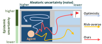
Figure 1: An intuitive example. The agent learns to move to the flag in a room filled with noise, and the noise in the left side is higher. The optimistic exploration strategy may overly explore the noisy area, and the risk-averse policy indiscriminately avoids noisy areas but explores insufficiently.

Therefore, a more reasonable approach is integrating the risk-averse policy and optimistic exploration, guiding the agent to optimistically exploring the whole areas, while avoiding overly exploring the areas with high noise, like the Ours arrow in Fig. 1. Note that overly exploring noisy areas may damage performance, but moderate exploration of such area is necessary, which should be ensured by the ability of optimistic exploration. The similar concern has been demonstrated to be effective under discrete control tasks (Nikolov et al. 2019; Clements et al. 2019). However, for continuous control tasks, such concern has not yet been investigated well. A natural way to apply discrete control algorithms to solve continuous control problems is to discretize the continuous action space, but it suffers from the scalability issue due to the exponentially increasing discretized actions (Antos, Munos, and Szepesvári 2007; Li et al. 2021), and it may throw away crucial information in action space causing its performance to be compromised (Lillicrap et al. 2016; Tang and Agrawal 2020). Thus, designing such an optimistic exploration strategy that can avoid overly exploring noisy area for continuous action space is required.

In this work, we propose OVD-Explorer, a noise-aware optimistic exploration strategy that applies to continuous control tasks for the first time. Specifically, we propose a new policy’s exploration ability measurement, quantifying both the ability of avoiding noise and pursuing optimisticity during exploration. To capture the noise, the value distribution is modelled. Further, to guide optimistic exploration, the upper bound distribution of return is approximated using Optimistic Value Distribution (OVD), representing the best returns that the policy can reach. Then we quantitatively measure such ability using OVD, and generates the behavior policy by maximizing the exploration ability measurement, thus names our approach as Optimistic Value Distribution Explorer (OVD-Explorer).

To make OVD-Explorer tractable for continuous control, we generate the behavior policy using a gradient-based approach, and propose a scheme to incorporate it with policy-based RL algorithms. Practically, we demonstrate the exploration benefits based on SAC (Haarnoja et al. 2018), a well-performed continuous RL algorithm. Evaluations on various continuous RL tasks, including the GridChaos, MuJoCo tasks and their stochastic version, are conducted. The results demonstrate the effectiveness of OVD-Explorer in achieving an optimistic exploration that avoids overly exploring noisy areas, leading to a better performance.

2 Related Work

In this work, we consider the exploration strategy under the OFU principle (Auer, Cesa-Bianchi, and Fischer 2002), and aim to a noise-aware optimistic exploration strategy.

Overview of exploration approaches. Basic exploration strategies always lead to undirected exploration through random perturbations (Lillicrap et al. 2016; Sutton and Barto 2018; Haarnoja et al. 2018). With the increasing emphasis on exploration efficiency in RL, various exploration methods have been developed (Hao et al. 2023). One kind of methods uses intrinsic motivation to stimulate agent to explore (Martin et al. 2017; Bellemare et al. 2016; Savinov et al. 2019; Houthooft et al. 2016; Badia et al. 2020; Yuan et al. 2023). Some other methods, originating from tracking uncertainty, guide exploration under the OFU principle (Thompson 1933; Osband et al. 2016; Nikolov et al. 2019; Ciosek et al. 2019; Pathak, Gandhi, and Gupta 2019; Bai et al. 2021b, a). The key of OFU-based exploration methods is modeling the epistemic uncertainty (Osband et al. 2016; Gal and Ghahramani 2016; Qiu et al. 2022). Specifically, we use ensemble (Osband et al. 2016) for estimating epistemic uncertainty.

The issue of overly exploring noisy areas. There is another uncertainty in RL system, i.e., aleatoric uncertainty (a.k.a. noise (Kirschner and Krause 2018) or risk (Dabney et al. 2018a)), captured by return distribution (Bellemare, Dabney, and Munos 2017; Dabney et al. 2018a, b). Overly exploring the areas with high noise could make learning unstable and inefficient, thus many works seek a conservative and noise-averse (or risk-averse) policy to make the policy stable (Dabney et al. 2018a; Ma et al. 2020; Bai et al. 2022). Nevertheless, conservative alone without advanced exploration could induce low exploration efficiency, and exploration without avoiding noise could make interaction risky. Thus some recent works produce optimistic exploration strategies considering risk (Mavrin et al. 2019; Nikolov et al. 2019). However, such methods are complicated when deriving a behavior policy and only limited to discrete control.

Indeed, addressing noise in exploration poses a challenge for well-performing continuous RL algorithms (Haarnoja et al. 2018; Ma et al. 2020). While exploration strategies like OAC (Ciosek et al. 2019) are designed following OFU principle, guided by the upper bound of $Q$ estimation, they overlook the potential impact of noise. This oversight can lead to misguided exploration, hampering the learning process. To address that, we propose OVD-Explorer to guide agent to explore optimistically, while avoiding overly exploring the noisy areas, improving the robustness of exploration especially facing heteroscedastic noise.

3 Preliminaries

Distributional Value Estimation

To capture the environment noise, we use quantile regression (Dabney et al. 2018b) to formulate $Q$-value distribution. $Q$-value distribution, represented by the quantile random variable $Z$, maps the state-action pair to a uniform probability distribution supported on the return values at all corresponding quantile fractions. Given state-action pair $(s,a)$, we denote the $i$-th quantile fraction as $\tau_{i}$, and the value at $\tau_{i}$ as $Z_{\tau_{i}}(s,a)$, where $\tau_{i}\in[0,1]$.

Based on the Bellman operator (Watkins and Dayan 1992), the distributional Bellman operator (Bellemare, Dabney, and Munos 2017) $\mathcal{T}_{D}^{\pi}$ under policy $\pi$ is given as:

$$\mathcal{T}_{D}^{\pi}Z(s,a)\stackrel{{\scriptstyle\mathclap{{D}}}}{{=}}R(s,a)+\gamma Z(s^{\prime},a^{\prime}),a^{\prime}\sim\pi(\cdot|s^{\prime}).$$ (1)

Notice that $\mathcal{T}_{D}^{\pi}$ operates on random variables, $\stackrel{{\scriptstyle\mathclap{{D}}}}{{=}}$ denotes that distributions on both sides have equal probability laws. Based on operator $\mathcal{T}_{D}^{\pi}$, QR-DQN (Dabney et al. 2018b) trains quantile estimations via the quantile regression loss (Koenker and Hallock 2001), which is denoted as:

$$\mathcal{L}_{QR}(\theta)=\frac{1}{N}\sum_{i=1}^{N}\sum_{j=1}^{N}[\rho_{\hat{\tau}_{i}}(\delta_{i,j})],$$ (2)

where $\theta$ and $\bar{\theta}$ is the parameters of the value distribution estimator and its target network, respectively, TD error $\delta_{i,j}=R(s,a)+\gamma{Z}_{\hat{\tau}_{i}}(s^{\prime},a^{\prime};\bar{\theta})-{Z}_{\hat{\tau}_{j}}(s,a;\theta)$, the quantile Huber loss $\rho_{\tau}(u)=u*|\tau-\mathds{1}_{u<0}|$, and $\hat{\tau}_{i}$ means the quantile midpoints, which is defined as $\hat{\tau}_{i}=\frac{\tau_{i-1}+\tau_{i}}{2}$.

Distributional Soft Actor-Critic

Distributional Soft Actor-Critic (DSAC) (Ma et al. 2020) seamlessly integrates distributional RL with Soft Actor-Critic (SAC) (Haarnoja et al. 2018). Basically, based on the Eq. 1, the distributional soft Bellman operator $\mathcal{T}^{\pi}_{DS}$ is defined considering the maximum entropy RL as follows:

$$\mathcal{T}^{\pi}_{DS}Z(s,a)\ \stackrel{{\scriptstyle\mathclap{{D}}}}{{=}}\ R(s,a)+\gamma[Z(s^{\prime},a^{\prime})-\alpha\log\pi(a^{\prime}|s^{\prime})],$$ (3)

where $a^{\prime}\sim\pi(\cdot|s^{\prime}),s^{\prime}\sim\mathcal{P}(\cdot|s,a)$. Then, to overcome overestimation of $Q$-value estimation, DSAC extends clipped double $Q$-Learning (Fujimoto, van Hoof, and Meger 2018), maintaining two critic estimators $\theta_{k},k=1,2$. Thus, the quantile regression loss differs from Eq. 2 on TD loss of $\theta_{l}$:

$$\delta_{i,j}^{l}= R(s,a)+\gamma[\min_{k=1,2}{Z}_{\hat{\tau}_{i}}(s^{\prime},a^{\prime};\bar{\theta}_{k})-\alpha\log\pi(a^{\prime}|s^{\prime};\bar{\phi})]$$ (4)

$$-{Z}_{\hat{\tau}_{j}}(s,a;\theta_{l}),$$

where $\bar{\theta}$ and $\bar{\phi}$ represents their target networks respectively. The objective of actor is the same as SAC,

$$\mathcal{J}_{\pi}(\phi)=\mathop{\mathbb{E}}\limits_{\begin{subarray}{c}s\sim\mathcal{D}\\ \epsilon\sim\mathcal{N}\end{subarray}}[\ \log\pi(f_{\phi}(s,\epsilon)|s)-Q(s,f_{\phi}(s,\epsilon);\theta)\ ],$$ (5)

where $\mathcal{D}$ is the replay buffer, $f_{\phi}(s,\epsilon)$ means sampling action with re-parameterized policy and $\epsilon$ is a noise vector sampled from any fixed distribution, like standard spherical Gaussian. Here, $Q$ value is the minimum value of the expectation on totally $N$ quantile fractions, as

$$Q(s,a;\theta)=\min_{k=1,2}{\mathbb{E}}_{i\sim\mathcal{U}(1,N)}{Z}_{\hat{\tau}_{i}}(s,a;\theta_{k}).$$ (6)

4 Optimistic Value Distribution Explorer

In noisy environments, a more efficient exploration strategy entails being noise-aware optimistic, especially to avoid excessive exploration in noisy areas. Over exploration towards the areas with high noise may damage the exploration performance, but indiscriminately avoiding visiting such areas could also compromise performance due to excessively conservation and insufficient exploration. In this work, we propose OVD-Explorer to achieve a noise-aware optimistic exploration in continuous RL. Accordingly, the key insight, theoretical derivation and formulation, and analysis of OVD-Explorer are outlined below.

Noise-aware Optimistic Exploration

Several previous optimistic exploration strategies for continuous control typically estimate the upper bound of $Q$-value, and guide exploration by maximizing this upper bound (Ciosek et al. 2019; Lee et al. 2021). While such upper bounds provide valuable guidance for optimistic exploration, they fail to capture the noise in the environment. To address that, we propose to incorporate the value distribution into the definition of the upper bound to capture noise, and define the upper bound distribution of $Q$-value. Additionally, we introduce a novel exploration ability measurement for policy distribution $\pi(\cdot)$ using such upper bound distribution, to characterize a policy’s ability for noise-aware optimistic exploration. We then derive the behavior (exploration) policy by maximizing this ability measurement.

Firstly, we define the upper bound distribution of the $Q$-value at each state-action pair as $\bar{Z}^{\pi}(s,a)$.

Definition 1 (The upper bound distribution of $Q$-value)

Given state-action pair $(s,a)$, the upper bound distribution of its $Q$-value, denoted as $\bar{Z}^{\pi}(s,a)$, is a value distribution satisfying that at each quantile fraction $\tau_{i}\in[0,1]$, its value $\bar{Z}^{\pi}_{\tau_{i}}(s,a)$ is the upper bound of possible estimations:

$$\bar{Z}^{\pi}_{\tau_{i}}(s,a):=\sup_{\theta}{Z}^{\pi}_{\tau_{i}}(s,a;\theta),$$ (7)

where $\theta$ represents different estimators of value distribution, ${Z}^{\pi}_{\tau_{i}}(s,a;\theta)$ represent the value at quantile fraction $\tau_{i}$ of the value distribution estimation ${Z}^{\pi}(s,a;\theta)$.

We expect an effective exploration policy to approach the upper bound of $Q$-value. With the distribution-based definition of such an upper bound, we then employ mutual information to evaluate the correlation between the policy distribution and the upper bound distribution, which forms the basis for our definition of exploration capability. Overall, given current state $s$, we quantitatively measure the policy’s exploration ability, denoted as ${\bf{F}}^{\pi}(s)$, by the integral of mutual-information between policy $\pi(\cdot|s)$ and the upper bound distributions of $Q$-value over the action space:

$${\bf{F}}^{\pi}(s)=\int_{a^{\prime}}{\bf{MI}}(\bar{Z}^{\pi}(s,a^{\prime});\pi(\cdot|s)|s)\mathop{}\!\mathrm{d}{a^{\prime}}$$ (8)

where $a^{\prime}\in\bf{A}$ denotes any legal action. Now we state how to approximate the exploration ability in Proposition 2.

Proposition 2

The mutual information in Eq. 8 at state $s$ can be approximated as:

$${\bf{F}}^{\pi}(s)\approx\frac{1}{C}\mathop{\mathbb{E}}_{\begin{subarray}{c}a\sim\pi(\cdot|s)\\ \bar{z}(s,a)\sim\bar{Z}^{\pi}(s,a)\end{subarray}}\left[\Phi_{Z^{\pi}}(\bar{z}(s,a))\log\frac{\Phi_{Z^{\pi}}(\bar{z}(s,a))}{C}\right].$$ (9)

$\Phi_{x}(\cdot)$ is the cumulative distribution function (CDF) of random variable $x$, $\bar{z}(s,a)$ is the sampled upper bound of return from its distribution $\bar{Z}^{\pi}(s,a)$ following policy $\pi$, $Z^{\pi}$ describes the current return distribution of the policy $\pi$, and $C$ is a constant (see proof in App. A).

Note that, to optimize the above objective, we need to formulate two critical components at any state-action pair $(s,a)$ under policy $\pi$: the return distribution $Z^{\pi}(s,a)$ and the upper bound distribution of return $\bar{Z}^{\pi}(s,a)$. We detail the formulations in Sec. 4.2.

Proposition 2 reveals that ${\bf{F^{\pi}}}(s)$ is only proportional to the CDF value $\Phi_{Z^{\pi}}(\bar{z}(s,a))$, which is also proportional to $\bar{z}(s,a)$, an upper bound of $Q$-value, thus a higher ${\bf{F^{\pi}}}(s)$ represents the higher ability of optimistic exploration, following traditional OFU principle. Meanwhile, $\Phi_{Z^{\pi}}(\bar{z}(s,a))$ increases as the variance of current return distribution $Z^{\pi}$ becomes lower, thus the higher ${\bf{F^{\pi}}}(s)$ means the higher ability of exploring towards the areas with low variance of return distribution, i.e., low noise. A more detailed analysis is given in Sec. 4.3.

Given current state $s$, OVD-Explorer aims to find the behavior policy $\pi_{E}$ which has the best exploration ability ${\bf{F^{\pi}}}(s)$ in the policy space $\Pi$, as follows:

$$\pi_{E}=\arg\max_{\pi\in\Pi}{\bf{F}}^{\pi}(s).$$ (10)

For continuous action space, generating the analytical solution $\pi_{E}$ in Eq. 10 is intractable. Hence, we propose to perform the gradient ascent based on the policy $\pi$, so as to iteratively deriving a behavior policy with high ability of noise-aware optimistic exploration. In short, given the policy $\pi_{\phi}$ parameterized by $\phi$, we calculate the derivative $\nabla_{\phi}\Phi_{Z^{\pi_{\phi}}}(\bar{z}(s,a))$ and guide $\phi$ along the gradient direction to improve the exploration ability (more details in Sec. 5).

Distributions of Return’s Upper Bound and Return

Now, we introduce the formulation of the return distribution $Z^{\pi}(s,a)$ and its upper bound distribution $\bar{Z}^{\pi}(s,a)$.

In specific, we use two value distribution estimators $\hat{Z}(s,a;\theta_{1})$ and $\hat{Z}(s,a;\theta_{2})$ parameterized by $\theta_{1}$ and $\theta_{2}$, as ensembles to formulate $\bar{Z}^{\pi}$ and $Z^{\pi}$ differently. Unless stated otherwise, $(s,a)$ is omitted hereafter to ease notation. As mentioned earlier, two types of uncertainties are involved, epistemic uncertainty and aleatoric uncertainty (noise), denoted as $\sigma_{\text{epistemic}}^{2}(s,a)$ and $\sigma_{\text{aleatoric}}^{2}(s,a)$, respectively. Due to space limitations, the computational details regarding uncertainty value are presented in detail in the appendix.

Formulation of $\bar{Z}^{\pi}$. The $\bar{Z}^{\pi}$ denotes the upper bound distribution of return that policy $\pi$ can reach. We propose Gaussian distribution with optimistic mean value $\mu_{\bar{Z}}(s,a)$ for formulation to formulate $\bar{Z}^{\pi}(s,a)$ as follows, and accordingly refer to it as Optimistic Value Distribution (OVD):

$$\bar{Z}^{\pi}(s,a)\sim\mathcal{N}(\mu_{\bar{Z}}(s,a),\sigma^{2}_{\text{aleatoric}}(s,a)),$$ (11)

where $\sigma^{2}_{\text{aleatoric}}(s,a)$ is its variance. Notable, Chen et al. (2017) discovers the optimisticity is beneficial for better estimating the upper bound, which motivates us to optimistically estimate $\mu_{\bar{Z}}(s,a)$ as averaged upper bound value of return by considering epistemic uncertainty as follows:

$$\mu_{\bar{Z}}(s,a)=\mu(s,a)+\beta\sigma_{\text{epistemic}}(s,a),\$$ (12)

$$\textup{s.t. }\mu(s,a)=\mathbb{E}_{i\sim\mathcal{U}(1,N)}\mathbb{E}_{k={1,2}}\hat{Z}_{\tau_{i}}(s,a;\theta_{k})$$

where $\mu(s,a)$ represents the expected $Q$-value estimation, and uncertainty value is weighted by $\beta$, $\mathcal{U}$ is uniform distribution, $N$ is the number of quantiles, and $\hat{Z}_{\tau_{i}}(s,a;\theta_{k})$ is the value of the $i$-th quantile drawn from $\hat{Z}(s,a;\theta_{k})$.

Leveraging optimistic value estimations together with explicitly modeling the noise, the upper bound distribution $\bar{Z}^{\pi}$ can be comprehensively formulated, known as OVD. Such an optimistic distribution can guides effectively optimistic exploration for OVD-Explorer.

Formulation of $Z^{\pi}$. $Z^{\pi}$ estimates the return distribution obtained following policy $\pi$. Following Fujimoto, van Hoof, and Meger (2018), to alleviate overestimation, we formulate $Z^{\pi}$ in a pessimistic way. In practice, $Z^{\pi}$ can be measured in two ways. First, similar to formulating $\bar{Z}^{\pi}$ in Eq. 11, $Z^{\pi}$ can also be formulated as Gaussian distribution as follows:

$$Z^{\pi}(s,a)\sim\mathcal{N}(\mu_{Z^{\pi}}(s,a),\sigma^{2}_{\text{aleatoric}}(s,a)),\quad$$ (13)

$$\textit{s.t.}\quad\mu_{Z^{\pi}}(s,a)=\mu(s,a)-\beta\sigma_{\text{epistemic}}(s,a),$$

where $\mu(s,a)$, $\sigma_{\text{aleatoric}}(s,a)$ and $\sigma_{\text{epistemic}}(s,a)$ are the same defined in Eq. LABEL:4-2-e13. Differently, $\sigma_{\text{epistemic}}(s,a)$ is subtracted from $\mu(s,a)$ to reveal the pessimistic estimation.

Another way is to formulate $Z^{\pi}$ pessimistically as multivariate uniform distribution as:

$$Z^{\pi}(s,a)\sim\mathcal{U}\{z^{\pi}_{i}(s,a;\theta)\}_{i=1,...,N},\quad$$ (14)

$$\textit{s.t.}\ z^{\pi}_{i}(s,a;\theta)=\min_{k={1,2}}\hat{Z}_{\tau_{i}}(s,a;\theta_{k}),$$

where each quantile value $z^{\pi}_{i}(s,a;\theta)$ is the minimum estimated value among ensemble estimators (i.e., $\hat{Z}_{\tau_{i}}(s,a;\theta_{k}$).

OVD-Explorer formulates the value distribution $Z^{\pi}$ in two ways using Eq. LABEL:4-2-e15 and Eq. 14, abbreviated in the following as OVDE_G and OVDE_Q, respectively. Intuitively, Gaussian distribution is expected to help more when the environment randomness follows a unimodal distribution, and multivariate uniform distribution is more flexible and suitable for scenarios with multi-modal distributions.

Analysis of OVD-Explorer

To analyzes how OVD-Explorer optimistically explores the whole areas and performs noise-aware exploration at the same time, an intuitive example involving two actions is adopted. According to Proposition 2, the behavior policy of OVD-Explorer maximizes $\mathbf{F}^{\pi}(s)$, which is proportional to the CDF value $\Phi_{Z^{\pi}}(\bar{z}(s,a))$. Supposing an agent need to select an actions between $a_{1}$ and $a_{2}$ to explore, Fig. 2(a) and (b) illustrate the CDF value (shaded area) for each action.

In these cases, the value distribution $Z^{\pi}(s,a)$ is specified as Gaussian (Eq. LABEL:4-2-e15), and the sampled optimistic value $\bar{z}(s,a)$ is specified as the mean of OVD $\mu_{\bar{Z}}(s,a)$ (Eq. LABEL:4-2-e13). At state $s$, we assume that the means of $Z^{\pi}$ at actions $a_{1}$ and $a_{2}$ are the same for ease of clarification.

Optimistic exploration: Fig. 2(a) illustrates how OVD-Explorer achieves an optimistic exploration. Assuming the noise at $a_{1}$ and $a_{2}$ is equal, but epistemic uncertainty is higher at $a_{1}$, then $\mu_{\bar{Z}}(s,a_{1})>\mu_{\bar{Z}}(s,a_{2})$ and the CDF value is larger at $a_{1}$. Therefore, OVD-Explorer prefers $a_{1}$ with high epistemic uncertainty for an optimistic exploration.

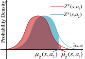
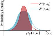
Figure 2: How OVD-Explorer explores (a) optimistically about epistemic uncertainty, (b) pessimistically about noise.

Noise-aware exploration: Fig. 2(b) demonstrates how OVD-Explorer behave noise-aware to avoid the area with higher noise (aleatoric uncertainty). When both actions have equal epistemic uncertainty, $\mu_{\bar{Z}}(s,a_{1})$ = $\mu_{\bar{Z}}(s,a_{2})$, and noise is lower at $a_{1}$ (PDF curve of $Z^{\pi}(s,a_{1})$ is “thinner and taller”), the CDF value will be larger at $a_{1}$. In such a case, OVD-Explorer prefers action $a_{1}$ with lower aleatoric uncertainty (i.e., lower noise) for a noise-aware exploration.

Adaptivity. In the early training, the noise estimations of all actions are nearly identical (Fig. 2(a)), and the exploration is primarily guided by epistemic uncertainty. After sufficient training, the epistemic uncertainty decreases, while the noise estimation converges to true environment randomness (Fig. 2(b)). At this point, exploration strategy tends to be noise-avoiding. OVD-Explorer seeks an adaptive balance of noise-aware optimistic exploration throughout the exploration process, which is a significant advantage compared to other OFU-based methods.

5 OVD-Explorer for RL Algorithms

For continuous RL, solving the argmax operator in Eq. 10 is intractable. In this section, aiming at maximizing ${\bf{F}}^{\pi}(s)$, we use a gradient-based approach to generate the behavior policy, and incorporate it with policy-based algorithms.

We denote the policy learned by any policy-based algorithm as $\pi_{\phi}$, parameterized by $\phi$. To avoid the gap between $\pi_{\phi}$ and the training data collected by behavior policy $\pi_{E}$, we derive $\pi_{E}$ in the vicinity of $\pi_{\phi}$. Then, aiming at maximizing ${\bf{F}}^{\pi_{\phi}}(s)$, we derive its gradient regarding the policy $\nabla_{\phi}{\bf{F}}^{\pi_{\phi}}(s)$ using automatic differentiation and generate behavior policy $\pi_{E}$ by performing gradient ascent based on $\pi_{\phi}$. Thus $\pi_{E}$ can guide exploration towards maximizing the exploration ability continuously, performing noise-aware optimistic exploration. Concretely, Proposition 3 shows how to calculate $\pi_{E}$.

Proposition 3

Based on any policy $\pi_{\phi}=\mathcal{N}(\mu_{\phi},\sigma_{\phi})$, the OVD-Explorer behavior policy $\pi_{E}=\mathcal{N}(\mu_{E},\Sigma_{E})$ at given state $s$ is as follows:

$$\mu_{E}=\mu_{\phi}+\alpha\mathbb{E}_{\bar{Z}^{\pi}}\left[m\times\frac{\partial\bar{z}(s,a)}{\partial a}|_{a=\mu_{\phi}}\right],$$ (15)

and

$$\Sigma_{E}=\sigma_{\phi}.$$ (16)

In specific, $m=\log\frac{\Phi_{Z^{\pi}(s,\mu_{\phi})}(\bar{z}(s,\mu_{\phi}))}{C}+1$, $\bar{z}(s,a)$ is a sample from OVD $\bar{Z}^{\pi}$, and $\alpha$ controls the step size of the update along the gradient direction, representing the exploration degree (see proof in App. A).

The expectation $\mathbb{E}_{\bar{Z}^{\pi}}$ can be estimated by K samples, then Eq. 15 is simplifies as:

$$\mu_{E}=\mu_{\phi}+\frac{\alpha m}{K}\sum_{i=1}^{K}\frac{\partial\bar{z}_{i}(s,a)}{\partial a}|_{a=\mu_{\phi}}.$$ (17)

Algorithm 1 Behavior policy generation at step $t$.

Input: Current state $s_{t}$, current value distribution estimators $\theta_{1},\theta_{2}$, current policy network $\phi$.
Output: Behavior policy $\pi_{E}$.

1:  Obtain policy $\pi_{\phi}(\cdot|s_{t})\sim\mathcal{N}(\mu_{\phi}(s_{t}),\sigma_{\phi}(s_{t}))$

2:  // Construct the distributions of return and upper bound

3:  Construct OVD $\bar{Z}^{\pi}(s_{t},\mu_{\phi}(s_{t}))$ using Eq. 11

4:  Construct $Z^{\pi}(s_{t},\mu_{\phi}(s_{t}))$ using Eq. LABEL:4-2-e15 or 14

5:  // Calculate the behavior policy

6:  Calculate the behavior policy’s mean $\mu_{E}$ using Eq. 17

7:  return $\pi_{E}\sim\mathcal{N}(\mu_{E},\sigma_{\phi}(s_{t}))$

Algorithm 1 summarizes the procedure to generate a behavior policy at step $t$ of OVD-Explorer. Following Algorithm 1, OVD-Explorer can be integrated with any existing policy-based RL algorithms from a distributional perspective, to render a stable and well-performed algorithm. Specifically, given state $s_{t}$, based on the current policy (Line 1), by constructing the optimistic value distribution $\bar{Z}^{\pi}$ as well as the value distribution $Z^{\pi}$ of the policy (Line 3-4), the behavior policy derived from OVD-Explorer can be calculated directly using Proposition 3 (Line 6-7).

6 Experiments

To reveal the consistency between our theoretical analysis and the performance of OVD-Explorer, and demonstrate the significant advantage over other advanced methods, we conduct experiments mainly for the following questions:
RQ1 (Exploration ability): Can OVD-Explorer explore as a noise-aware optimistic manner as expected?
RQ2 (Performance): Can OVD-Explorer perform notable advantages on common continuous control benchmarks?
Due to space constraints, more experimental details and evaluation results can be found in the appendix.

Baseline Algorithms and Implementation Details

Our baseline algorithms include SAC (Haarnoja et al. 2018), DSAC (Ma et al. 2020), and DOAC, an extension of the scalar Q-value within the OAC (Ciosek et al. 2019) to distributional Q-value. Our implementation of OVD-Explorer is based on the OAC repository, also refers to the code of DSAC and softlearning . We implement OVD-Explorer_G and OVD-Explorer_Q (or abbreviated as OVDE_G and OVDE_Q), representing approaches to formulate the value distribution $Z^{\pi}$ using Eq. LABEL:4-2-e15 (torch.distributions.Normal) or Eq. 14, respectively. The key hyper-parameters associated with the exploration, i.e., the exploration ratio $\alpha$ and the uncertainty ratio $\beta$, are determined by grid search, with detailed information presented in the Appendix. Moreover, the hyperparameters related to the training procedure remain consistent across all algorithms.

All experiments are performed on NVIDIA GeForce RTX 2080 Ti 11GB graphics card. To counteract the randomness from a statistical perspective, we conduct multiple trials using different seeds. The final results of each trial are collected based on the mean undiscounted episodic return over the last 8% epoch (or up to the last 100 epochs) to ensure impartiality and minimize bias.

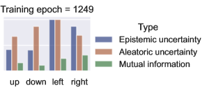
Figure 3: GridChaos. Left: In this map, the areas with darker background color have higher noise injected, and the agent aims at reaching the goal at the top right. Right: The values of uncertainty and exploration ability.

Exploration in GridChaos (RQ1)

To illustrate that OVD-Explorer guides noise-aware optimistic exploration, we first evaluate OVD-Explorer on GridChaos. The GridChaos task is characterized by heterogeneous noise and sparse reward, making it particularly challenging and necessitating a robust capacity for noise-aware optimistic exploration to successfully accomplish the task.

GridChaos Task

GridChaos is built on OpenAI’s Gym toolkit, as shown in Fig. 3(a). In GridChaos, the cyan triangle is under the agent’s control, with the objective of reaching the fixed dark blue goal located at the top right corner. The state is its current coordinate, and the action is a two-dimensional vector including the movement angle and distance. An episode terminates when the agent reaches the goal or maximum steps (typically 100). Also, it receives a +100 reward when reaching the goal, and otherwise 0. To simulate noise, heterogeneous Gaussian noise is injected into the state transitions. Fig. 3(b) shows a basic performance comparison of algorithms, and show our advantage. More detailed performance are illustrated in the following.

Exploration Patterns Analysis

We first analyse the exploration pattern facilitated by OVD-Explorer. We compare values of uncertainty and the exploration ability measurement (in Proposition 2) corresponding to distinct actions at the state in Fig. 3(a). Fig. 3(c) shows the values obtained at the 1249th training epoch. Basically, Fig. 3(c) shows that estimated aleatoric uncertainty (noise) of left is the highest, aligning with the environment’s inherent attribute. This indicates that OVD-Explorer models the noise properly. Further, OVD-explorer encourages to explore towards right, where the exploration ability (in green) is higher. It implies that OVD-explorer balances the optimistic and noise in exploration, aligning with our intended objective. Nevertheless, if the noise is not considered in exploration, the agent would be guided towards left, where the epistemic uncertainty is higher, then the agent may be trapped due to the high randomness in this area, potentially explaining why DOAC fails to effectively address such a stochastic task.

Evaluation on Various Noise Scales

To further empirically prove our strength, we test OVD-Explorer in GridChaos with various noise scales settings, as outlined in row A-E in Tab. 1. The column Noise setup shows different scale of environmental heterogeneous Gaussian noise injected in four quadrants of Cartesian coordinate system. Note that the variance is not reported, as the mean values offer a comprehensive representation of results across 5 seeds. For instance, when the average result approaches 20, it indicates that only one seed successfully achieved the goal (obtaining a reward of +100) in the end. The row S is the standard GridChaos as shown in Fig. 3(a). Note that OVDE-m is specifically designed for the second set of experiment (see Sec. 6), thus we omit its results in this experiment. Remarkably, the results indicate that OVD-Explorer consistently achieves better performance across all the tested settings, particularly in scenarios with high levels of noise. This underscores OVD-Explorer’s exploration capability in such noisy tasks, leading to more efficient learning and faster convergence towards the goal (see column FRG).

Also, we make observations in the case without noise (row E). Here, DSAC fails in any run across 5 seeds, while DOAC reachs the goal in one run but at a slower pace. OVD-Explorer achieves the goal swiftly in one run. This highlight the capability of OVD-Explorer and the highly challenging nature of the task, emphasizing the significance of employing a robust exploration strategy.

	Noise setup				Average return			FRG epoch
	1	2	3	4	DSAC	OVDE	DOAC	DSAC	OVDE	DOAC
s	0.1	0.5	0.5	0.1	0.00	59.30	3.02	1250+	229	1222
a	0.0	0.5	0.1	0.1	18.94	58.99	38.42	1161	180	662
b	0.0	0.05	0.01	0.01	39.78	79.52	18.71	694	144	846
c	0.05	0.1	0.1	0.05	0.05	39.64	20.59	1250+	180	309
d	0.001	0.005	0.005	0.001	20.00	40.46	39.99	284	276	321
e	0.0	0.0	0.0	0.0	0.00	20.20	14.60	1250+	185	1118

Table 1: The averaged return of 5 runs for GridChaos (the first part). FRG epoch means the minimum training epochs to Firstly Reach the Goal before totally 1250 epochs.

	Noise setup				Average return				FRG epoch
	1	2	3	4	DSAC	OVDE	OVDE(m)	DOAC	DSAC	OVDE	DOAC
f	0.1	0.05	0.05	0.1	0.00	19.84	39.96	20.14	1250+	188	233
g	0.05	0.005	0.005	0.05	0.00	20.69	20.07	0.00	1250+	247	1250+
h	0.01	0.005	0.005	0.01	0.0	40.00	60.00	39.99	1250+	200	301
i	0.005	0.001	0.001	0.005	20.00	39.98	20.00	20.00	236	312	296

Table 2: The averaged return of 5 runs (the second part).

Task	Epoch	SAC		DSAC		DOAC		OVD-Explorer_G		OVD-Explorer_Q
Ant-v2	2500	4867.	8$\pm$1658.7	6385.	9$\pm$1287.2	6625.	4$\pm$746.8	7175.	3$\pm$789.0	7382.	3$\pm$466.6
HalfCheetah-v2	2500	11619.	8$\pm$1642.01	13348.	4$\pm$1957.1	12987.	6$\pm$148.1	14796.	2$\pm$1473.2	16484.	3$\pm$1373.75
Hopper-v2	1250	2593.	5$\pm$574.7	2506.	0$\pm$390.56	2353.	0$\pm$754.1	2394.	6$\pm$496.6	2559.	3$\pm$384.5
Reacher-v2	250	-22.	7$\pm$2.0	-12.	2$\pm$1.6	-18.	7$\pm$1.7	-11.	6$\pm$1.0	-11.	3$\pm$1.2
InvDbPendulum-v2	300	9306.	2$\pm$89.5	8916.	9$\pm$1041.7	5798.	5$\pm$3439.0	9263.	8$\pm$189.1	9355.	0$\pm$12.1
N-Ant-v2	2500	222.	96$\pm$41.93	465.	34$\pm$53.94	344.	71$\pm$20.39	524.	16$\pm$10.54	513.	77$\pm$17.87
N-HalfCheetah-v2	1250	368.	57$\pm$28.01	431.	81$\pm$39.41	402.	26$\pm$37.27	447.	3$\pm$38.57	453.	56$\pm$55.97
N-Hopper-v2	1250	213.	71$\pm$21.97	238.	62$\pm$19.89	252.	53$\pm$13.07	234.	88$\pm$15.24	239.	43$\pm$9.90
N-Pusher-v2	1250	-50.	57$\pm$20.65	-27.	33$\pm$3.79	-29.	82$\pm$4.29	-25.	69$\pm$3.57	-26.	13$\pm$3.63
N-InvDbPendulum-v2	300	931.	63$\pm$7.14	932.	81$\pm$1.87	381.	87$\pm$139.36	932.	70$\pm$2.26	933.	54$\pm$2.69
Average (standard tasks)		5672.92		6229.00		5549.16		6723.66		7153.92
Average (noisy tasks)		337.26		408.25		270.31		422.67		422.83

Table 3: Comparisons of algorithms on five standard and five noisy tasks. The averaged performance and standard deviation of 10 runs are reported. The training epoch count is shown in column epoch, and the best values of each row are shown in bold.

Evaluation on Tasks in Which the Noise is High around the Goal

To verify whether the noise avoidance ability of OVD-Explorer dominates the exploration process when the noise around the target is higher, we conduct the experiment where the noise in the right half (where the goal is located), is set larger. The results are shown in row F-G in Tab. 2. Note that we use OVDE to denote the usual implementation that pessimistically estimates the value distribution (i.e., using Eq. LABEL:4-2-e15). Besides, OVDE(m) denotes the implementation that does not pessimistically estimate the value distribution (i.e., we modify the mean of Gaussian distribution $Z^{\pi}$ in Eq. LABEL:4-2-e15 from the lower bound to expected value of the $Q$ estimation $\mu(s,a)$ as in Eq. LABEL:4-2-e13).

Overall, in most cases, OVD-Explorer guides better exploration and perform better than baselines. This highlights OVD-Explorer’s ability to handle various scenarios effectively, even in tasks with higher noise levels around the goal.

Moreover, an intriguing observation is that OVD-Explorer may exhibit better performance when the pessimistic estimation is turned off in the presence of higher noise around the goal (see column OVDE(m)). This finding suggests that excessive pessimism may not be necessary when there is a crucial need to explore areas characterized by high aleatoric uncertainty. In such cases, a more balanced approach may lead to improved results.

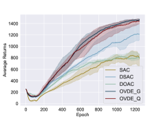
(a) 250 steps

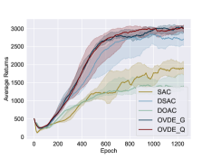
(b) 500 steps

Figure 4: Training curves on Noisy Ant-v2 tasks with different maximum episodic length setup. The sub-title of each figure represents the episodic horizon. We report the median of returns and the interquartile range of 10 runs. Curves are smoothed uniformly for visual clarity.

Performance on Mujoco Tasks (RQ2)

To showcase the broader efficacy of OVD-Explorer, we conduct experiments encompassing 5 standard and 5 stochastic tasks based on wildly-used continuous control benchmark, Gym Mujoco. Tab. 3 shows the averaged performance and standard deviation of 10 seeds. It is important to note that for the standard tasks, the dynamics are deterministic, and any observed noise is ascribed to the stochastic policy employed. Conversely, in the case of the five noisy tasks (indicated by the prefix N-), Gaussian noise of varying scales is randomly injected into each state transition. The investigation yields compelling insights into the capabilities of OVD-Explorer.

Primarily, OVD-Explorer can perform stably in standard task. The results reveal that DSAC consistently outperforms SAC, underscoring the advantage that value distribution brings to policy evaluation. Notably, OVD-Explorer surpasses baseline algorithms significantly, particularly in high-dimensional tasks, such as Ant-v2 and HalfCheetah-v2. These evaluations on standard tasks convincingly demonstrate OVD-Explorer’s remarkable proficiency in promoting optimistic exploration, highlighting its universal efficacy in exploration capabilities.

Second, these results underscore the efficacy of OVD-Explorer in exploring noisy environments while avoiding the adverse impact of noise. This is exemplified by experiments on 5 noisy tasks (Tab. 3) and Noisy Ant-v2 tasks with varying maximum episodic lengths (Fig. 6, detailed results in the appendix). Notably, DOAC’s performance is even inferior to DSAC in most tasks, indicating that the presence of heteroscedastic noise significantly interferes with the exploration process guided by DOAC. In contrast, OVD-Explorer exhibits substantial advantages over SAC and DOAC, notably outperforming DSAC in most cases.

Furthermore, regarding the two implementations (namely OVDE_G and OVDE_Q) of OVD-Explorer, we observe that OVDE_Q consistently demonstrates greater stability. The key distinction between these implementations lies in the formulations of $Z^{\pi}(s,a)$. OVDE_Q’s employment of quantile distribution offers higher flexibility, allowing for a more accurate characterization of the value distribution. Conversely, OVDE_ G, reliant on the Gaussian prior, exhibits limited capacity in this regard, leading to a relatively diminished performance in some cases.

7 Conclusion

In this paper, we have presented OVD-Explorer, a novel noise-aware optimistic exploration method for continuous RL. By introducing a unique measurement of exploration ability and maximizing it, OVD-Explorer effectively generates a behavior policy that adheres to the OFU principle. Also, it intelligently avoids excessive exploration in areas with high noise, thereby mitigating the adverse effects of noise. Consistently across tasks with no noise as well as various forms of noise, the experiment underscores our performance advantages. Moving forward, we recognize the potential for extending OVD-Explorer to discrete tasks and even Multi-agent tasks. This will enhance the versatility of OVD-Explorer, affording it the capability to effectively confront the challenges of exploration in noisy environments that are widespread across diverse real-world scenarios.

8 Acknowledgments

This work is supported by the National Key R&D Program of China (Grant No. 2022ZD0116402), the National Natural Science Foundation of China (Grant Nos. 92370132, 62106172).

Appendix A Proof of Proposition 2 and Proposition 3

In this appendix we prove Proposition 2 and Proposition 3.

Proof of Proposition 2

In order to prove the Proposition 2, we first propose the following lemma about ${\bf{F^{\pi}}}(s)$.

Lemma 4

The integral of all mutual information between upper bound distribution of legal action $\bar{Z}^{\pi}(s,a^{\prime})$ and policy $\pi(\cdot|s)$ at state $s$, i.e. ${\bf{F}}^{\pi}(s)$ , is:

$${\bf{F}}^{\pi}(s) =\int\limits_{\begin{subarray}{c}a\end{subarray}}\mathop{\mathbb{E}}_{\begin{subarray}{c}\bar{z}(s,a)\\ \sim\bar{Z}^{\pi}(s,a)\end{subarray}} \left[p(a|\bar{z}(s,a),s)\log\frac{p(a|\bar{z}(s,a),s)}{\pi(a|s)}\right]\mathop{}\!\mathrm{d}{a},$$ (18)

where $p(a|\bar{z}(s,a),s)$ represents the posterior probability distribution of policy given current state $s$ and the sampled upper bound of return $\bar{z}(s,a)$.

Proof  From the definition of mutual information, Eq. 8 is immediately given as:

$${\bf{F}}^{\pi}(s)$$ (19)

$$= \int\limits_{\begin{subarray}{c}a^{\prime}\end{subarray}}\int\limits_{\begin{subarray}{c}a\end{subarray}}\int\limits_{\begin{subarray}{c}\bar{z}(s,a^{\prime})\end{subarray}}\left[p(a,\bar{z}(s,a^{\prime})|s)\log\frac{p(a,\bar{z}(s,a^{\prime})|s)}{p(\bar{z}(s,a^{\prime}))\pi(a|s)}\right]$$

$$\mathop{}\!\mathrm{d}{\bar{z}(s,a^{\prime})}\mathop{}\!\mathrm{d}{a}\mathop{}\!\mathrm{d}{a^{\prime}}$$

$$= \int\limits_{\begin{subarray}{c}a^{\prime}\end{subarray}}\int\limits_{\begin{subarray}{c}a\end{subarray}}\int\limits_{\begin{subarray}{c}\bar{z}(s,a^{\prime})\end{subarray}}\Biggl{[}p(\bar{z}(s,a^{\prime}))p(a|\bar{z}(s,a^{\prime}),s)$$

$$\log\frac{p(\bar{z}(s,a^{\prime}))p(a|\bar{z}(s,a^{\prime}),s)}{p(\bar{z}(s,a^{\prime}))\pi(a|s)}\Biggr{]}\mathop{}\!\mathrm{d}{\bar{z}(s,a^{\prime})}\mathop{}\!\mathrm{d}{a}\mathop{}\!\mathrm{d}{a^{\prime}}$$

$$= \int\limits_{\begin{subarray}{c}a^{\prime}\end{subarray}}\int\limits_{\begin{subarray}{c}a\end{subarray}}\mathop{\mathbb{E}}_{\begin{subarray}{c}\bar{z}(s,a^{\prime})\\ \sim\bar{Z}^{\pi}(s,a^{\prime})\end{subarray}}\left[p(a|\bar{z}(s,a^{\prime}),s)\log\frac{p(a|\bar{z}(s,a^{\prime}),s)}{\pi(a|s)}\right]\mathop{}\!\mathrm{d}{a}\mathop{}\!\mathrm{d}{a^{\prime}},$$

where the posterior distribution $p(a|\bar{z}(s,a^{\prime}),s)$ is the probability of choosing action $a$ on the condition of the samples from upper bounds of action $a^{\prime}$.

Considering that for making decision, the probability of action $a$ is independent to the values of other actions, which means that

$$p(a|\bar{z}(s,a^{\prime}),s)=\begin{cases}\pi(a|s)&a\neq a^{\prime},\\ p(a|\bar{z}(s,a),s)&a=a^{\prime}.\end{cases}$$ (20)

Therefore, Eq. LABEL:eq-proof-theorem1-1 can be further reduced as follows:

$${\bf{F}}^{\pi}(s)=\int\limits_{\begin{subarray}{c}a\end{subarray}}\mathop{\mathbb{E}}_{\begin{subarray}{c}\bar{z}(s,a)\\ \sim\bar{Z}^{\pi}(s,a)\end{subarray}} \left[p(a|\bar{z}(s,a),s)\log\frac{p(a|\bar{z}(s,a),s)}{\pi(a|s)}\right]\mathop{}\!\mathrm{d}{a}.$$

 
Lemma 4 tells that ${\bf{F^{\pi}}}(s_{t})$ is in direct proportion to $p(a|\bar{z}(s,a),s)$, which measures how much it is worth acting under the current policy $\pi(a|s)$ when the upper bound is known.

Next, to measure the posterior probability $p(a|\bar{z}(s,a),s)$, we use a practically effective approach of approximating the posterior probability given upper bound value (Wang and Jegelka 2017; Belakaria, Deshwal, and Doppa 2020; Perrone et al. 2019; Li et al. 2020).

Specifically, we approximate $p(a|\bar{z}(s,a),s)$ using the prior that $z^{\pi}(s,a)\leq\bar{z}(s,a)$ with given policy $\pi(s,a)$, since $\bar{z}(s,a)$ is the upper bound of $z^{\pi}(s,a)$. Hence, we use the indicator function $\mathds{1}_{z^{\pi}(s,a)\leq\bar{z}(s,a)}$ to truncate the policy $\pi(s,a)$, and utilize the constant C to normalize the probability, as is shown in the following equation.

$$p(a|\bar{z}(s,a),s)\approx\frac{1}{C}\pi(a|s)\mathbb{E}_{z^{\pi}(s,a)\sim Z^{\pi}(s,a)}\left[\mathds{1}_{z^{\pi}(s,a)\leq\bar{z}(s,a)}\right].$$

Here, $\mathbb{E}_{z^{\pi}(s,a)\sim Z^{\pi}(s,a)}\left[\mathds{1}_{z^{\pi}(s,a)\leq\bar{z}(s,a)}\right]={\Phi_{Z^{\pi}(s,a)}}(\bar{z}(s,a))$, where $\Phi_{x}$ is the cumulative distribution function (CDF) of $x$, $\bar{Z}^{\pi}$ and $Z^{\pi}$ are the random variables, whose distributions describe the randomness of the returns, and $\bar{z}(s,a)$ is the value of random variable $\bar{Z}^{\pi}$. Therefore, the posterior probability can be measured as follows,

$$p(a|\bar{z}(s,a),s)\approx\frac{1}{C}\pi(a|s)\Phi_{Z^{\pi}}(\bar{z}(s,a)).$$ (21)

In our method, we do not use approximation mechanisms about mutual information such as neural network estimation (Belghazi et al. 2018) and upper bound estimation (Cheng et al. 2020). Instead, we find the correlation between random variables as shown in Eq. 21, which helps to approximate mutual information directly.

According to Lemma 4 and Eq. 21, we can give the proof of Proposition 2 in the following.

Proof  By Combining Lemma 4 and Eq. 21, ${\bf{F^{\pi}}}(s)$ can be further derived as follows.

$${\bf{F}}^{\pi}(s)$$

$$\approx \int_{\begin{subarray}{c}a\sim\pi(\cdot|s)\end{subarray}}\mathop{\mathbb{E}}_{\bar{z}(s,a)\sim\bar{Z}^{\pi}(s,a)}\Biggl{[}\frac{1}{C}\pi(a|s)\Phi_{Z^{\pi}}(\bar{z}(s,a))$$

$$\log\frac{\pi(a|s)\Phi_{Z^{\pi}}(\bar{z}(s,a))}{C\pi(a|s)}\Biggr{]}\mathop{}\!\mathrm{d}{a}$$

$$= \frac{1}{C}\mathop{\mathbb{E}}_{\begin{subarray}{c}a\sim\pi(\cdot|s)\\ \bar{z}(s,a)\sim\bar{Z}^{\pi}(s,a)\end{subarray}}\left[\Phi_{Z^{\pi}}(\bar{z}(s,a))\log\frac{\Phi_{Z^{\pi}}(\bar{z}(s,a))}{C}\right]$$

Here, the last equality follows from Proposition 2.  

Proof of Proposition 3

Proof  Similar to (Ciosek et al. 2019), we set the covariance matrix of $\pi_{E}$ is that of $\pi_{\phi}$, i.e., $\Sigma_{E}=\sigma_{\phi}$. Hence, the OVD-Explorer problem is simplified as finding the $\mu$ that maximizes $\mathbf{\hat{F}}^{\pi}(s,\mu)$:

$$\mathbf{\hat{F}}^{\pi}(s,\mu)=\mathop{\mathbb{E}}_{\bar{Z}^{\pi}}\left[\Phi_{Z^{\pi}}(\bar{z}(s,\mu))\log\frac{\Phi_{Z^{\pi}}(\bar{z}(s,\mu))}{C}\right]$$

To ensure that $\pi_{E}$ samples actions around $\pi_{\phi}$, we derive $\pi_{E}$ upon mean $\mu_{\phi}$ of target policy $\pi_{\phi}$. In specific, we firstly obtain the gradient of $\mathbf{\hat{F}}(s,\mu)$ at $\pi_{\phi}$, which is given as follows:

$$\nabla_{a}\mathbf{\hat{F}}^{\pi}(s,\mu)|_{\mu=\mu_{\phi}}=\mathbb{E}_{\bar{Z}^{\pi}}\left[\hat{m}\times\frac{\partial\bar{z}(s,a)}{\partial a}|_{a=\mu_{\phi}}\right]$$

where $\hat{m}=\phi_{Z^{\pi}(s,\mu_{\phi})}(\bar{z}(s,\mu_{\phi}))(\log\frac{\Phi_{Z^{\pi}(s,\mu_{\phi})}(\bar{z}(s,\mu_{\phi}))}{C}+1)$, and $\phi(x)$ is the probability distribution function (pdf). Hence, $\mu_{E}$ is given as follows:

$$\mu_{E}=\mu_{\phi}+\alpha\mathbb{E}_{\bar{Z}^{\pi}}\left[m\times\frac{\partial\bar{z}(s,a)}{\partial a}|_{a=\mu_{\phi}}\right],$$

where $\alpha$ is the step size controlling exploration level and $m=\log\frac{\Phi_{Z^{\pi}(s,\mu_{\phi})}(\bar{z}(s,\mu_{\phi}))}{C}+1$.  

Appendix B Details about OVD-Explorer

The formulation of uncertainties

Our proposed method considers two types of uncertainty that exist within the RL system, both of which play a crucial role in our approach. Below, we elaborate on the formulation of these uncertainties.

The epistemic uncertainty characterizes the ambiguity of the model arisen from insufficient knowledge, and it tends to be high at state-action pairs that are rarely visited. To estimate the epistemic uncertainty, we leverage the disagreement among ensemble estimators (Osband et al. 2016):

$$\sigma_{\text{epistemic}}^{2}(s,a)=\mathbb{E}_{i\sim\mathcal{U}(1,N)}\text{var}_{k=1,2}\hat{Z}_{\tau_{i}}(s,a;\theta_{k}),$$ (22)

where $\mathcal{U}$ is uniform distribution, $N$ is the number of quantiles, and $\hat{Z}_{\tau_{i}}(s,a;\theta_{k})$ is the value of the $i$-th quantile drawn from $\hat{Z}(s,a;\theta_{k})$.

The aleatoric uncertainty (noise) arises from the randomness in the environment, which can be attributed to the stochastic nature of policies, rewards, and/or transition probabilities. To model the aleatoric uncertainty (noise), we consider the variance of the value distribution $\bar{Z}^{\pi}$ (Clements et al. 2019) as follows:

$$\sigma_{\text{aleatoric}}^{2}(s,a)=\text{var}_{i\sim\mathcal{U}(1,N)}\left[\mathbb{E}_{k=1,2}\hat{Z}_{\tau_{i}}(s,a;\theta_{k})\right].$$ (23)

Algorithm 2: OVD-Explorer for SAC

the behavior policy generated by OVD-Explorer can be seamlessly integrated with existing policy-based RL algorithms from a distributional perspective, thereby promoting stable and effective exploration. For this purpose, in the context of SAC, we need to estimate the value distribution, resulting in the distributional variant of SAC, referred to as DSAC (Ma et al. 2020). Subsequently, we replace the behavior policy with the one generated by Algorithm 1 to interact with the environment. The complete algorithm for our implementation of OVD-Explorer based on SAC is presented in Algorithm 2. The entire code can be accessed in the supplementary material.

Algorithm 2 OVD-Explorer for DSAC

1:  Initialise: Value networks $\theta_{1}$, $\theta_{2}$, policy network $\phi$ and their target networks $\bar{\theta}_{1}$, $\bar{\theta}_{2}$, $\bar{\phi}$, quantiles number N, target smoothing coefficient ($\tau$), discount ($\gamma$), an empty replay pool $\mathcal{D}$

2:  for each iteration do

3:     for each environmental step do

4:        $a_{t}\sim\pi_{E}(a_{t},s_{t})$ according to Algorithm 1

5:        $\mathcal{D}\leftarrow\mathcal{D}\cup\{(s_{t},a_{t},r(s_{t},a_{t}),s_{t+1})\}$

6:     end for

7:     for each training step do

8:        for i = 1 to N do

9:           for j = 1 to N do

10:              calculate $\delta_{i,j}^{k},k={1,2}$, following Eq. 4

11:           end for

12:        end for

13:        Calculate $\mathcal{L}_{QR}(\theta_{k}),k={1,2}$ using $\delta_{i,j}^{k}$ following Eq. 2

14:        Update $\theta_{k}$ with $\nabla\mathcal{L}_{QR}(\theta_{k})$

15:        Calculate $\mathcal{J}_{\pi}(\phi)$, following Eq. 5

16:        Update $\phi$ with $\nabla\mathcal{J}_{\pi}(\phi)$

17:     end for

18:     Update target value network with $\bar{\theta}_{k}\leftarrow\tau\theta_{k}+(1-\tau)\bar{\theta}_{k},k=1,2$

19:     Update target policy network with $\bar{\phi}\leftarrow\tau\phi+(1-\tau)\bar{\phi}$

20:  end for

Appendix C Detailed Experimental Settings

Baseline Algorithms and Implementation Details

As mentioned in Sec 5, OVD-Explorer can be integrated with any policy-based DRL algorithm, such as SAC (Haarnoja et al. 2018) or TD3 (Fujimoto, van Hoof, and Meger 2018), by constructing optimistic and current value distributions reasonably. In this paper, we implement OVD-Explorer based on SAC. In the following, we first elaborate on the baseline algorithms and implementation details for better reproducibility.

The baseline algorithms include SAC (Haarnoja et al. 2018), DSAC (Ma et al. 2020), and DOAC. (Ma et al. 2020) has compared the performance of the distributional extension of SAC and TD4 (i.e., DSAC and TD4, respectively), showing that DSAC outperforms TD4 on Mujoco tasks. Thus, we implement OVD-Explorer based on SAC to show its advantage of exploration, comparing with SAC and DSAC. Besides, DOAC, the distributional variant of OAC (Ciosek et al. 2019), performing optimistic exploration but ignoring the noise, is involved to illustrate the necessity of noise-aware exploration.

SAC. We implement SAC (Haarnoja et al. 2018) based on the OAC repository. The results in Ant-v2 and Hopper-v2 are similar to reported results, and we report a better result than OAC’s implementation for SAC on HalfCheetah-v2.

DSAC. DSAC is implemented based on SAC, except that the distributional $Q$ function is used instead of the traditional $Q$ function in SAC. We set same hyper-parameters for DSAC and SAC to ensure a fair comparison. In our results, DSAC can guarantee an absolute advantage over SAC in most cases, which is consistent with the previous conclusion.

DOAC. We implement DOAC based on DSAC as well as the OAC repository. As DSAC shows great advantage due to the distributional value estimation, to ensure a fair comparison, we extend OAC (Ciosek et al. 2019) to its distributional version, i.e., DOAC, by replacing the exploration process of DSAC by the behavior policy derived by OAC. We set the hyper-parameters the same as used by OAC in Mujoco, and our results of DOAC on Ant-v2 and HalfCheetah-v2 are significantly better than that OAC reported.

Finally, we illustrate the summary of the baselines with respect to the optimistic and noise-aware exploration in Table 4. OVD-Explorer possesses both of these essential exploration attributes, making it a promising and effective method in noisy environments. DOAC demonstrates optimistic exploration but lacks noise-aware capabilities. DSAC and SAC, on the other hand, do not exhibit either optimistic or noise-aware exploration characteristics.

Table 4: Summary of OVD-Explorer and baselines regarding to the optimistic and risk-averse exploration.

Algorithm	Optimistic	Risk-Averse
OVD-Explorer	$\checkmark$	$\checkmark$
DOAC	$\checkmark$	$\times$
DSAC	$\times$	$\times$
SAC	$\times$	$\times$

	Parameter		Value
Training	Discount		0.99
	Target smoothing coefficient	$\tau$	5e-3
	Learning rate		3e-4
	Optimizer		Adam (Kingma and Ba 2015)
	Batch size		256
	Quantiles amount		20
	Replay buffer size		$1.0\times 10^{6}$ for Mujoco tasks
			$1.0\times 10^{5}$ for other tasks
	Environment steps per epoch		$1.0\times 10^{3}$ for Mujoco tasks
			$1.0\times 10^{2}$ for other tasks
Exploration	Exploration ratio	$\alpha$	0.05 (specified otherwise)
	Uncertainty ratio	$\beta$	3.2
	Normalization factor	$C$	0.5

Table 5: Hyper-parameters in OVD-Explorer

Hyper-parameters

We illustrate the gyper-parameters used for training and exploration in Table 5.

Appendix D Discussions about other related works

Mutual information used in exploration. Following OFU principle, OVD-Explorer uses mutual information to define exploration ability for guiding exploration. There are some other information-theoretic exploration strategies, such as VIME (Houthooft et al. 2016), which measures the information gain on environment dynamics, and EMI (Kim et al. 2019), generating intrinsic reward using prediction error of representation learned by mutual information. which can solve sparse reward problem well using intrinsic reward. Nevertheless, those methods use mutual information neither on the value distribution, nor for OFU-based exploration. Besides, instead of using the mechanisms for approximating mutual information (Rakelly et al. 2021), such as variational inference (Hinton and van Camp 1993; Houthooft et al. 2016) or f-divergence (Nowozin, Cseke, and Tomioka 2016; Kim et al. 2019), we find the correlation between policy and upper bounds distribution through uncertainty, which helps estimate mutual information directly.

Safe exploration. Another related line of work focuses on risk-averse exploration or safe exploration, from the perspective of safe RL. Those methods design exploration strategies to achieve risk-averse policy (i.e., CVaR policy) (Greenberg et al. 2022; Keramati et al. 2020), or the policy with safety constraint (Dalal et al. 2018; Ding et al. 2021). Those methods have a fundamental difference with our approach. Specifically, our method aims to train the policy that maximizes expected return, concerned with the optimistic exploration in complex stochastic continuous control tasks, rather than a safe policy.

Appendix E More Results

In this section, we present a more comprehensive set of experimental results, covering various aspects that are not included in the main text due to space constraints. The additional results are as follows:

1. Time Consumption: We provide an analysis of the time consumption of OVD-Explorer in comparison to the baseline algorithms.

2. Hyperparameter Sensitivity: We investigate the impact of the two hyperparameters in OVD-Explorer and their influence on the algorithm’s performance.

3. Comparison with Non-Uncertainty-Based Strategies: We compare OVD-Explorer with other non-uncertainty-based exploration strategies to demonstrate its superiority in handling noisy environments effectively.

4. Results on Harder Noisy Tasks: We showcase the performance of OVD-Explorer on more challenging noisy tasks to assess its robustness in highly complex environments.

5. Exploration Patterns Visualization: We visualize the exploration patterns of OVD-Explorer by tracking state space visitation frequencies and similar measures. This provides insights into how the algorithm adapts its exploration strategy during the learning process.

6. Comparison of Exploration Patterns: We analyze the differences in exploration patterns between scenarios with high and low noise levels near the goal in the GridChaos task. This analysis sheds light on how OVD-Explorer explores noisy regions differently depending on the noise intensity.

Runtime Analysis

Method	Relative Runtime Time
SAC	1.0
DSAC	1.17
DOAC	1.19
OVDE_G	1.17
OVDE_Q	1.21

Table 6: Computational costs.

Table 6 shows the time consumption of algorithms relative to SAC. As can be seen, the distributional value estimation used in DSAC, DOAC and our methods introduces extra time consumption distinctly. Nevertheless, the relative time consumption of OVDE_G and OVDE_Q spends approximately 17% to 21% more time than SAC to achieve a significant performance gain of nearly 100%, as demonstrated in Figure 6(b). This indicates that the extra time consumption of OVD-Explorer is well justified by the substantial improvement in exploration efficiency. Besides, the time consumption of OVDE_Q is close to that of DSAC, with only a slightly larger variance. This suggests that the additional time consumption of OVDE_Q is minimal while still achieving better exploration performance, making it a promising choice for practical applications.

Task	DSAC	DSAC+RND	IDS	OVDE_G	OVDE_Q
Ant-v2	6385.9$\pm$1287.2	7308.4$\pm$641.3	503.2$\pm$23.3	7175.3$\pm$789.0	7382.3$\pm$466.6
HalfCheetah-v2	13348.4$\pm$1957.1	12198.1$\pm$2338.3	203.3$\pm$33.2	14796.2$\pm$1473.2	16484.3$\pm$1373.75
Hopper-v2	2506.0$\pm$390.56	2077.9$\pm$344.1	1201.0$\pm$42.2	2394.6$\pm$496.6	2559.3$\pm$384.5
N-HalfCheetah-v2	431.81$\pm$39.41	409.48$\pm$45.88	68.3$\pm$21.3	447.3$\pm$38.57	453.56$\pm$55.97
N-Hopper-v2	236.62$\pm$19.89	231.46$\pm$9.94	136.3$\pm$58.1	234.88$\pm$15.24	239.43$\pm$9.90
N-Ant-v2 (250)	1217.87$\pm$185.00	1306.05$\pm$223.18	36.3$\pm$63.1	1434.61$\pm$113.53	1340.00$\pm$221.64

Table 7: Comparisons with IDS and RND. For DSAC+RND and IDS, the averaged performance and standard deviation of 5 runs are reported.

Sensitivity to $\alpha$ and $\beta$

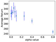
(a) $\alpha$ value

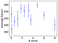
(b) $\beta$ value

Figure 5: Sensitivity to (a) $\alpha$ and (b) $\beta$. The x-axis indicates values of hyper-parameters, while the y-axis is the evaluation result represented by average episode return and half standard deviation (error bars) over 5 seeds. The 9 different $\alpha$ values are 0.0005, 0.01. 0.025, 0.05, 0.075, 0.1, 0.25, 0.4, 0.8, respectively. The 11 different $\beta$ values are 0.05, 0.1, 0.6, 1.2, 1.8, 2.4, 3.2, 3.6, 4.8, 6.0, 8.0.

To determine the appropriate values for the hyperparameters $\alpha$ and $\beta$ in OVD-Explorer, we conduct experiments to investigate their impact on the algorithm’s performance.

For the hyperparameter $\alpha$, which controls the distance between the exploration policy $\pi_{E}$ derived from OVD-Explorer and the given policy $\pi_{\phi}$, we test several $\alpha$ values on the Noisy Ant-v2 task using OVDE_G. The results are shown in Fig. 5(a). It is observed that the performance of OVD-Explorer varies with different $\alpha$ values. If $\alpha$ is too small, OVD-Explorer degenerates to DSAC and lacks optimistic exploration. Conversely, if $\alpha$ is too large, the performance worsens due to a substantial gap between $\pi_{E}$ and $\pi_{\phi}$. However, there exists a concentrated range of $\alpha$ values that facilitate more efficient exploration. In our experiments, we uniformly use $\alpha=0.05$ to showcase the performance of OVD-Explorer.

Regarding the hyperparameter $\beta$, which controls the scale of uncertainty quantification in Eq. LABEL:4-2-e13 and Eq. LABEL:4-2-e15, influencing $\bar{Z}^{\pi}$ and $Z^{\pi}$, we conduct experiments on the Noisy Ant-v2 task using OVDE_G. The sensitivity analysis of $\beta$ is illustrated in Fig. 5(b). The results demonstrate a broad range of suitable values for $\beta$ that lead to good performance. For our experiments, we set $\beta$ uniformly to be 3.2.

Comparison with Other Similar Algorithms

OVD-Explorer achieves optimistic noise-aware exploration, and outperforms the baseline algorithms including SAC, DSAC and DOAC. Additionally, there are other algorithms that share similar or partial objectives with OVD-Explorer, such as optimistic exploration based on intrinsic motivation and optimistic noise-aware exploration for discrete control. To provide a comprehensive comparison, we evaluate OVD-Explorer against these algorithms on three standard Mujoco tasks and three noisy Mujoco tasks, as shown in Table 7.

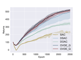
(a) 100 steps

(b) 250 steps

(c) 500 steps

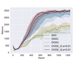
(d) 500 steps

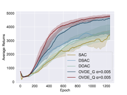
(e) 750 steps

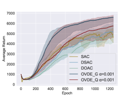
(f) 1000 steps

Figure 6: Training curves on Noisy Ant-v2 tasks with different maximum episodic length setup. The sub-title of each figure represents the episodic horizon, also known as the maximum episode length. We report the median of returns and the interquartile range of 10 runs. Curves are smoothed uniformly for visual clarity.

RND

Indeed, RND also follows the principle of Optimism in the Face of Uncertainty (OFU) and utilizes uncertainty estimation through network distillation to drive intrinsic motivation for agent exploration. To ensure fairness in comparison, we implement RND based on DSAC, denoted as DSAC+RND, and present the results in the DSAC+RND column of Table 7.

The results clearly indicate that OVD-Explorer maintains a significant performance advantage over DSAC+RND. While DSAC+RND shows promising results on the Ant-v2 task, it does not perform as well on other tasks. This performance gap can be attributed to two main factors.

Firstly, intrinsic motivation-based exploration methods, like RND, are known to exhibit some instability and sensitivity to the scale of intrinsic reward signals. This instability can result in varying performance when applied to different tasks, leading to inconsistent outcomes. Secondly, RND focuses primarily on episodic uncertainty, which may not be as effective in tasks that involve random noise, where the algorithm lacks the ability to adequately manage aleatoric uncertainty. In contrast, OVD-Explorer’s ability to handle both episodic and aleatoric uncertainty gives it an edge in effectively addressing noisy exploration challenges.

Noise-aware Optimistic Exploration for Discrete Control

For discrete control problems, IDS (Nikolov et al. 2019) exhibits similar optimistic exploration abilities as OVD-Explorer and can also avoid the negative impact of heterogeneous noise. However, it is important to note that IDS is specifically designed for discrete control tasks and may face limitations when applied to continuous control problems.

To assess the performance of IDS in solving continuous control problems, we discretize the continuous action space and present the evaluation results in the IDS column of Table 7. The results demonstrate that especially on tasks with larger action dimensions, IDS performs extremely poorly due to dimension explosion.

This observation highlights the significance of designing exploration strategies tailored for continuous reinforcement learning, such as OVD-Explorer. OVD-Explorer’s ability to guide optimistic exploration while avoiding excessive exploration in noisy areas proves essential for achieving robust and efficient exploration in continuous control tasks. As evidenced by the results, algorithms like OVD-Explorer play a crucial role in addressing the unique challenges posed by continuous control problems and outperforming approaches designed solely for discrete control scenarios.

Evaluation on Harder Noisy Tasks in Mujoco

Horizon	$\alpha$	SAC	DSAC	DOAC	OVDE_G	OVDE_Q
100	0.05	222.96±41.93	465.34±53.94	344.71±20.39	524.16±10.54	513.77±17.87
		<0.001	0.013	<0.001	-	0.406
250	0.05	764.93±159.5	1217.87±185.00	840.26±115.91	1434.61±113.53	1340.00±221.64
		<0.001	0.002	<0.001	-	0.414
500	0.05	1788.01±480.22	2613.02±400.11	1523.75±368.39	2864.40±351.54	2951.81±230.41
		<0.001	0.035	<0.001	0.194	-
500	0.01	1788.01±480.22	2613.02±400.11	1523.75±368.39	2831.99±283.31	3006.58±78.92
		<0.001	0.030	<0.001	0.619	-
750	0.005	3208.58±676.28	3932.89±738.76	3601.00±557.70	4207.39±721.80	4469.29±744.26
		<0.001	0.146	0.003	0.330	-
1000	0.001	4628.31±891.77	5214.21±1126.09	4926.53±1027.08	6214.59±791.73	5663.66±1134.54
		0.027	0.095	0.048	-	0.504

Table 8: Comparisons of algorithms on Noisy Ant-v2 tasks with different maximum episodic length setup. The averaged performance and standard deviation of 10 runs are reported, as well as the p-value that indicates the statistical significance of the difference between the proposed algorithm and each baseline algorithm. The best values of each row are shown in bold.

In Section 6, we demonstrate the significant advantage of OVD-Explorer over DSAC and DOAC in stochastic Mujoco tasks. To further empirically verify the efficiency of OVD-Explorer, we detail the evaluation on Noisy Ant-v2 task with different maximum episodic length setup. The results presented in Figure 6 and Table 8 illustrate that OVD-Explorer consistently outperforms the baseline algorithms across various maximum episodic lengths. Notably, longer maximum episodic lengths present higher task difficulty, particularly for high-dimensional tasks that demand more thorough exploration. From these experiments, we draw two key conclusions:

Firstly, these results further demonstrate the effectiveness of OVD-Explorer in exploring noisy environments. Figure 6 shows the training curves on Noisy Ant-v2 tasks, including the error bars of interquartile range. Tab. 8 reports the average results and standard deviation, and p-values to show if a significant difference exists comparing baselines. Notably, most p-values comparing OVD-Explorer’s performance to baseline algorithms are below 0.05, confirming that OVD-Explorer consistently and efficiently explores noisy environments across different levels of task difficulty.

Secondly, a practical finding is that exploration should be more conservative in harder tasks, where a smaller value of $\alpha$ in OVD-Explorer should be used. In Fig. 6(a), (b) and (c), $\alpha$ is set to 0.05 by default. In Fig. 6(d), (e), and (f), a smaller $\alpha$ is employed to achieve better performance in the more challenging tasks.

These empirical results further reinforce the superiority of OVD-Explorer in effectively addressing exploration challenges in noisy environments with varying degrees of difficulty. This makes it a practical and robust solution for continuous RL tasks with uncertainties and noise.

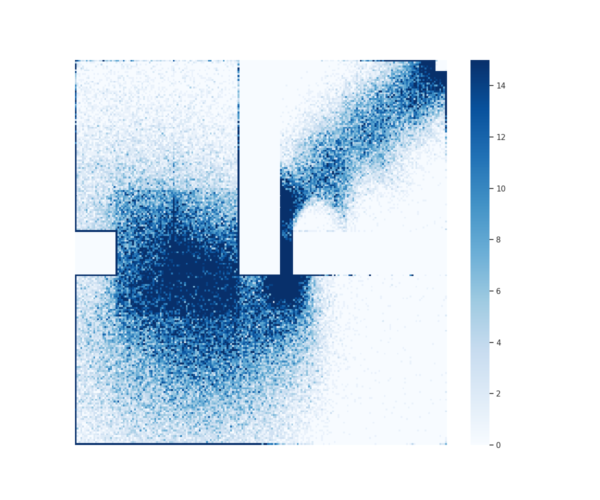
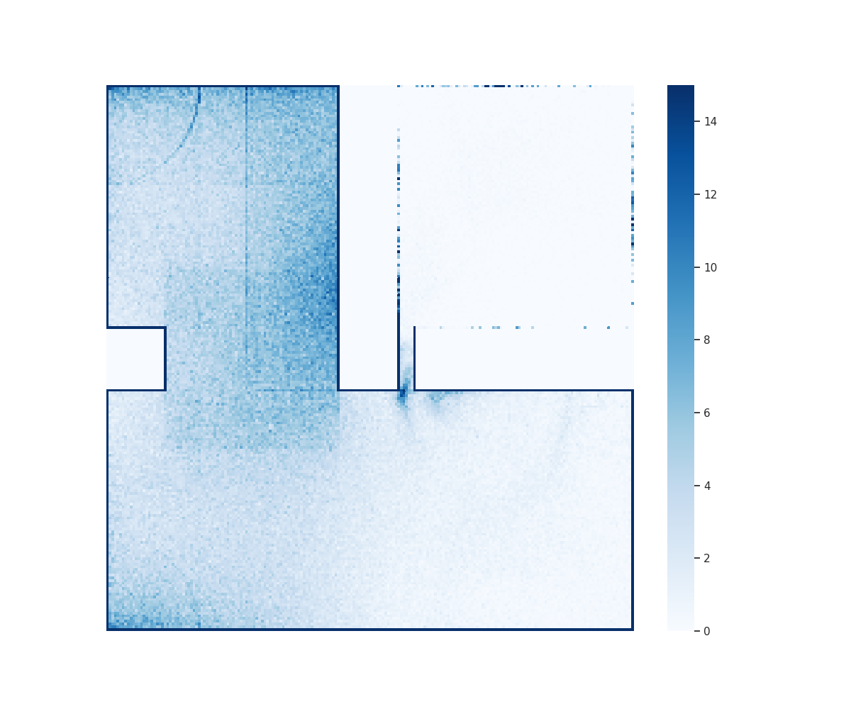
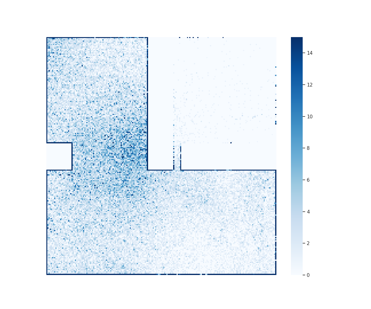
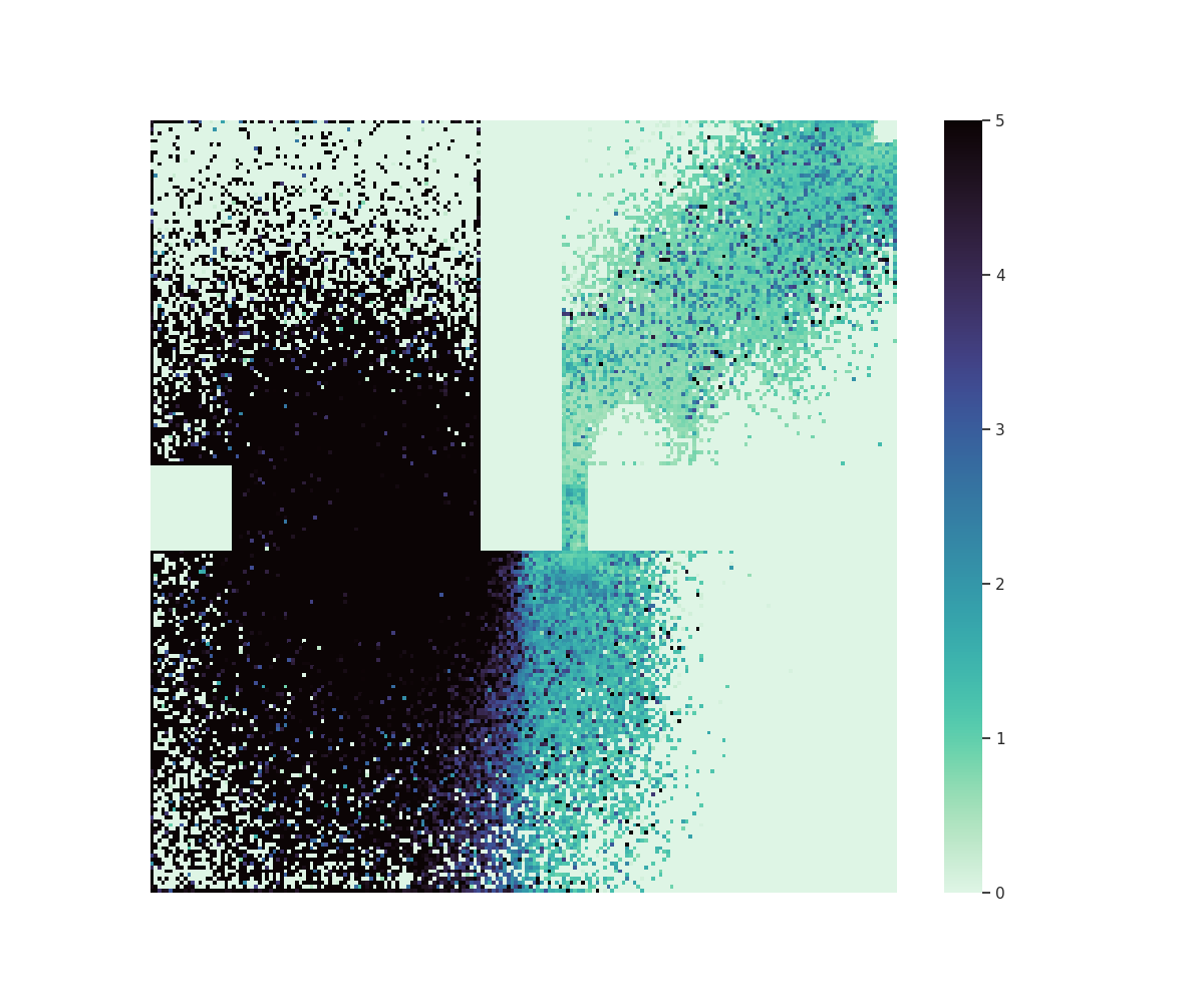
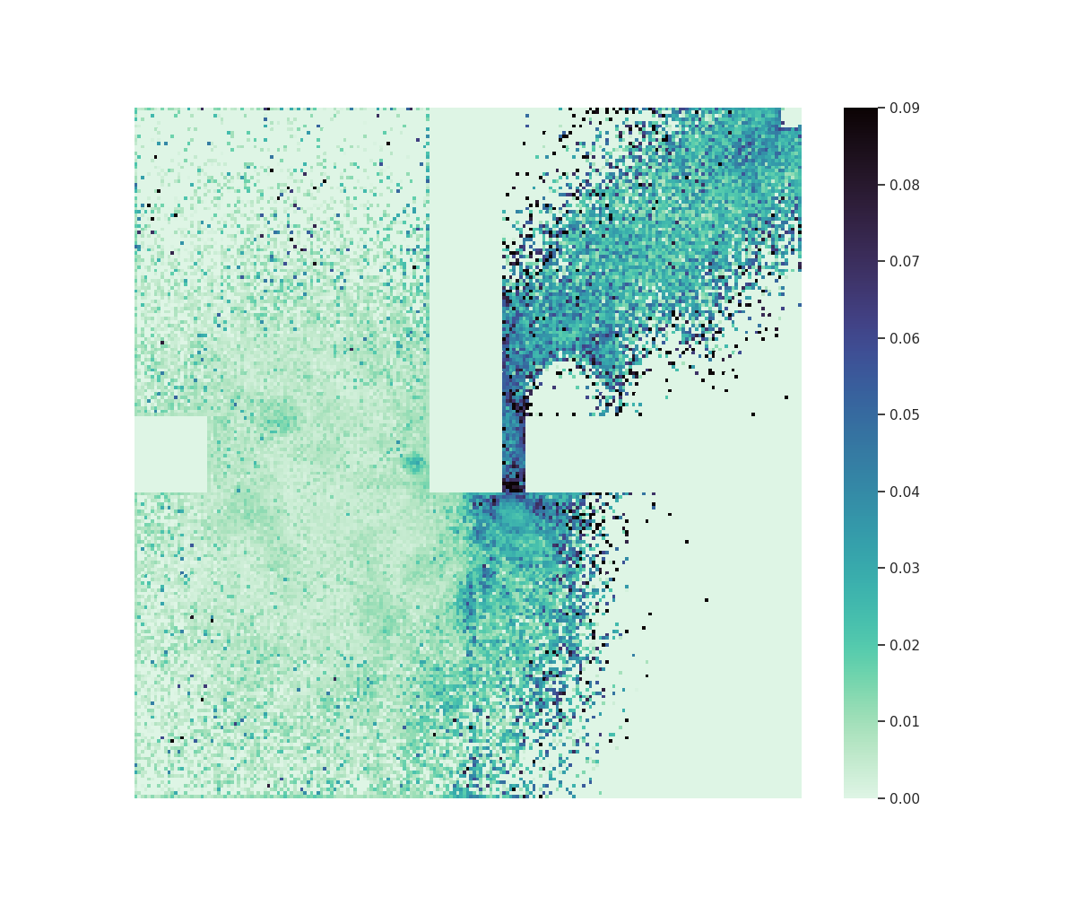
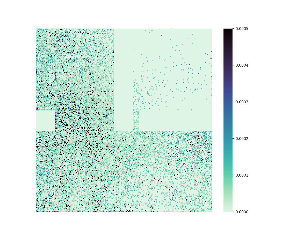
Figure 7: State visiting frequency heatmap from $1.0\times 10^{5}$ to $2.5\times 10^{5}$ steps of one trial for (a) OVD-Explorer, (b) DSAC and (c) DOAC. (d) Estimated aleatoric uncertainty of OVD-Explorer; (e) Epistemic-aleatoric ratio of OVD-Explorer; (f) Estimated uncertainty for exploration in DOAC.

Exploration Patterns Visualization in the Case of GridChaos

In this section, we provide a visual analysis of the exploration patterns and advantages of OVD-Explorer compared to DSAC and DOAC in the GridChaos task.

To begin with, we present heatmaps showing the state visiting frequency during exploration for OVD-Explorer, DSAC, and DOAC in Figures 7, 7 and 7, respectively. From these heatmaps, we observe distinct exploration patterns. OVD-Explorer efficiently explores the right half of the environment, where the environmental risk is lower, while DSAC and DOAC are both trapped in the left half, characterized by higher risk. In contrast, Figure 7 shows the estimated uncertainty in DOAC, which is larger on the left half. As DOAC encourages exploration in areas with relatively large estimated uncertainty, it explains why DOAC is stuck in the left half of the environment.

This visual analysis provides clear evidence of OVD-Explorer’s ability to efficiently explore the environment by effectively balancing optimistic and noise-aware exploration based on accurate uncertainty estimations. The comparison with DSAC and DOAC further illustrates the significant advantage of OVD-Explorer in tackling exploration challenges in noisy environments.

Analysis about Exploration Process of OVD-Explorer

In this section, we conduct a statistical analysis to further verify that OVD-Explorer can effectively perform optimistic noise-aware exploration. We show the values of uncertainty estimations and our exploration objective (mutual information) at different stages during the training processes of two trials with different noise settings.

Figure 8 illustrates the exploration process in a trial with lower environment noise around the goal, noting that the darker background color in the map represents higher noise, and the red dot represents the coordinate of the current state. The performance under this trail is given and the agent hardly ever reaches the goal before the 1000th epoch. Therefore, in the early stage, the aleatoric uncertainty is inaccurate and remains very low, as the value distribution shows little divergence. The figure also shows that our exploration objective (in green) is high when the epistemic uncertainty is high. So before the 1000th epoch, the exploration is guided by epistemic uncertainty, which follows the OFU principle. As the agent explores further and begins to properly model the aleatoric uncertainty, i.e., the aleatoric uncertainty towards left is larger than right at current state (see epoch 1240). Then the mutual information value towards left is lower than right, although the epistemic towards left is higher. It indicates that OVD-Explorer can property guide noise-aware optimistic exploration.

Figure 9 shows the exploration process in a trial with higher environment noise around the goal. Similarly to the previous case, the early stages of exploration are guided by epistemic uncertainty. The agent would hardly estimate the accurate aleatoric uncertainty without obtaining any reward. Later, as the agent explores more and gains a better understanding of the environment, at the 1240th epoch, OVD-Explorer suggests exploring to the right, even though it has been recognized that the noisy on the right is high. This is because the epistemic uncertainty dominates under the mutual information at that time. In contrast, at the 1249th epoch, when the action towards right has been explored much, the significant higher aleatoric uncertainty towards right dominates. Therefore, following the mutual information, the action towards left is preferred. This demonstrates the trade off that OVD-Explorer make, performing noise-aware optimistic exploration.

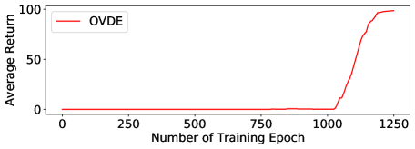
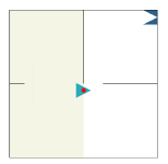
Figure 8: The statistical analysis for the training process, with the aleatoric uncertainty around the goal is set lower.

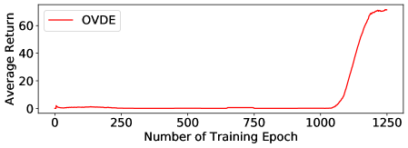
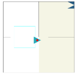
Figure 9: The statistical analysis for the training process, with the aleatoric uncertainty around the goal is set higher.

References

- Antos, Munos, and Szepesvári (2007) Antos, A.; Munos, R.; and Szepesvári, C. 2007. Fitted Q-iteration in continuous action-space MDPs. In Advances in NIPS, Vancouver, British Columbia, Canada, December 3-6, 2007, 9–16. Curran Associates, Inc.
- Auer, Cesa-Bianchi, and Fischer (2002) Auer, P.; Cesa-Bianchi, N.; and Fischer, P. 2002. Finite-time Analysis of the Multiarmed Bandit Problem. Mach. Learn., 47(2-3): 235–256.
- Badia et al. (2020) Badia, A. P.; Sprechmann, P.; Vitvitskyi, A.; Guo, D.; Piot, B.; Kapturowski, S.; Tieleman, O.; Arjovsky, M.; Pritzel, A.; Bolt, A.; and Blundell, C. 2020. Never Give Up: Learning Directed Exploration Strategies. arXiv preprint arXiv:2002.06038.
- Bai et al. (2021a) Bai, C.; Wang, L.; Han, L.; Garg, A.; Hao, J.; Liu, P.; and Wang, Z. 2021a. Dynamic bottleneck for robust self-supervised exploration. In Advances in Neural Information Processing Systems, volume 34, 17007–17020.
- Bai et al. (2021b) Bai, C.; Wang, L.; Han, L.; Hao, J.; Garg, A.; Liu, P.; and Wang, Z. 2021b. Principled Exploration via Optimistic Bootstrapping and Backward Induction. In International Conference on Machine Learning, volume 139, 577–587.
- Bai et al. (2022) Bai, C.; Xiao, T.; Zhu, Z.; Wang, L.; Zhou, F.; Garg, A.; He, B.; Liu, P.; and Wang, Z. 2022. Monotonic quantile network for worst-case offline reinforcement learning. IEEE Transactions on Neural Networks and Learning Systems.
- Belakaria, Deshwal, and Doppa (2020) Belakaria, S.; Deshwal, A.; and Doppa, J. R. 2020. Max-value Entropy Search for Multi-Objective Bayesian Optimization with Constraints. CoRR, abs/2009.01721.
- Belghazi et al. (2018) Belghazi, M. I.; Baratin, A.; Rajeswar, S.; Ozair, S.; Bengio, Y.; Hjelm, R. D.; and Courville, A. C. 2018. Mutual Information Neural Estimation. In ICML 2018, Stockholmsmässan, Stockholm, Sweden, volume 80, 530–539. PMLR.
- Bellemare, Dabney, and Munos (2017) Bellemare, M. G.; Dabney, W.; and Munos, R. 2017. A Distributional Perspective on Reinforcement Learning. In Proceedings of the 34th ICML, ICML 2017, Sydney, NSW, Australia, 6-11 August 2017, volume 70 of Proceedings of Machine Learning Research, 449–458. PMLR.
- Bellemare et al. (2016) Bellemare, M. G.; Srinivasan, S.; Ostrovski, G.; Schaul, T.; Saxton, D.; and Munos, R. 2016. Unifying Count-Based Exploration and Intrinsic Motivation. In Advances in NIPS, 1471–1479.
- Chen et al. (2017) Chen, R. Y.; Sidor, S.; Abbeel, P.; and Schulman, J. 2017. UCB exploration via Q-ensembles. arXiv preprint arXiv:1706.01502.
- Cheng et al. (2020) Cheng, P.; Hao, W.; Dai, S.; Liu, J.; Gan, Z.; and Carin, L. 2020. CLUB: A Contrastive Log-ratio Upper Bound of Mutual Information. In ICML 2020, 13-18 July 2020, Virtual Event, volume 119 of Proceedings of Machine Learning Research, 1779–1788. PMLR.
- Ciosek et al. (2019) Ciosek, K.; Vuong, Q.; Loftin, R.; and Hofmann, K. 2019. Better Exploration with Optimistic Actor Critic. In Advances in NeurIPS 2019, 8-14 December 2019, Vancouver, BC, Canada, 1785–1796.
- Clements et al. (2019) Clements, W. R.; Robaglia, B.; Delft, B. V.; Slaoui, R. B.; and Toth, S. 2019. Estimating Risk and Uncertainty in Deep Reinforcement Learning. CoRR, abs/1905.09638.
- Dabney et al. (2018a) Dabney, W.; Ostrovski, G.; Silver, D.; and Munos, R. 2018a. Implicit Quantile Networks for Distributional Reinforcement Learning. In Proceedings of the 35th ICML, ICML 2018, Stockholmsmässan, Stockholm, Sweden, July 10-15, 2018, volume 80 of Proceedings of Machine Learning Research, 1104–1113. PMLR.
- Dabney et al. (2018b) Dabney, W.; Rowland, M.; Bellemare, M. G.; and Munos, R. 2018b. Distributional Reinforcement Learning With Quantile Regression. In AAAI, New Orleans, Louisiana, USA, February 2-7, 2018, 2892–2901. AAAI Press.
- Dalal et al. (2018) Dalal, G.; Dvijotham, K.; Vecerík, M.; Hester, T.; Paduraru, C.; and Tassa, Y. 2018. Safe Exploration in Continuous Action Spaces. CoRR, abs/1801.08757.
- Ding et al. (2021) Ding, D.; Wei, X.; Yang, Z.; Wang, Z.; and Jovanovic, M. R. 2021. Provably Efficient Safe Exploration via Primal-Dual Policy Optimization. In AISTATS 2021, April 13-15, 2021, Virtual Event, volume 130 of Proceedings of Machine Learning Research, 3304–3312. PMLR.
- Fujimoto, van Hoof, and Meger (2018) Fujimoto, S.; van Hoof, H.; and Meger, D. 2018. Addressing Function Approximation Error in Actor-Critic Methods. In Proceedings of the 35th ICML, ICML 2018, Stockholmsmässan, Stockholm, Sweden, July 10-15, 2018, volume 80 of Proceedings of Machine Learning Research, 1582–1591. PMLR.
- Gal and Ghahramani (2016) Gal, Y.; and Ghahramani, Z. 2016. Dropout as a Bayesian Approximation: Representing Model Uncertainty in Deep Learning. In Proceedings of the 33nd ICML, ICML 2016, New York City, NY, USA, June 19-24, 2016, volume 48 of JMLR Workshop and Conference Proceedings, 1050–1059. JMLR.org.
- Greenberg et al. (2022) Greenberg, I.; Chow, Y.; Ghavamzadeh, M.; and Mannor, S. 2022. Efficient Risk-Averse Reinforcement Learning.
- Haarnoja et al. (2018) Haarnoja, T.; Zhou, A.; Abbeel, P.; and Levine, S. 2018. Soft Actor-Critic: Off-Policy Maximum Entropy Deep Reinforcement Learning with a Stochastic Actor. In ICML 2018, Stockholmsmässan, Stockholm, Sweden, July 10-15, 2018, volume 80 of Proceedings of Machine Learning Research, 1856–1865. PMLR.
- Hao et al. (2023) Hao, J.; Yang, T.; Tang, H.; Bai, C.; Liu, J.; Meng, Z.; Liu, P.; and Wang, Z. 2023. Exploration in deep reinforcement learning: From single-agent to multiagent domain. IEEE Transactions on Neural Networks and Learning Systems.
- Hinton and van Camp (1993) Hinton, G. E.; and van Camp, D. 1993. Keeping the Neural Networks Simple by Minimizing the Description Length of the Weights. In Proceedings of the Sixth Annual ACM Conference on Computational Learning Theory, COLT 1993, Santa Cruz, CA, USA, July 26-28, 1993, 5–13. ACM.
- Houthooft et al. (2016) Houthooft, R.; Chen, X.; Duan, Y.; Schulman, J.; De Turck, F.; and Abbeel, P. 2016. Vime: Variational information maximizing exploration. In Advances in NIPS, 1109–1117.
- Keramati et al. (2020) Keramati, R.; Dann, C.; Tamkin, A.; and Brunskill, E. 2020. Being Optimistic to Be Conservative: Quickly Learning a CVaR Policy. In AAAI 2020, New York, NY, USA, February 7-12, 2020, 4436–4443. AAAI Press.
- Kim et al. (2019) Kim, H.; Kim, J.; Jeong, Y.; Levine, S.; and Song, H. O. 2019. EMI: Exploration with Mutual Information. In ICML 2019, 9-15 June 2019, Long Beach, California, USA, volume 97 of Proceedings of Machine Learning Research, 3360–3369.
- Kingma and Ba (2015) Kingma, D. P.; and Ba, J. 2015. Adam: A Method for Stochastic Optimization. In ICLR 2015, San Diego, CA, USA, May 7-9, 2015, Conference Track Proceedings.
- Kirschner and Krause (2018) Kirschner, J.; and Krause, A. 2018. Information Directed Sampling and Bandits with Heteroscedastic Noise. In Conference On Learning Theory, COLT 2018, Stockholm, Sweden, 6-9 July 2018, volume 75 of Proceedings of Machine Learning Research, 358–384. PMLR.
- Koenker and Hallock (2001) Koenker, R.; and Hallock, K. F. 2001. Quantile regression. Journal of economic perspectives, 15(4): 143–156.
- Lee et al. (2021) Lee, K.; Laskin, M.; Srinivas, A.; and Abbeel, P. 2021. SUNRISE: A Simple Unified Framework for Ensemble Learning in Deep Reinforcement Learning. In ICML 2021, 18-24 July 2021, Virtual Event, volume 139 of Proceedings of Machine Learning Research, 6131–6141. PMLR.
- Li et al. (2021) Li, B.; Tang, H.; Zheng, Y.; Hao, J.; Li, P.; Wang, Z.; Meng, Z.; and Wang, L. 2021. HyAR: Addressing Discrete-Continuous Action Reinforcement Learning via Hybrid Action Representation. CoRR, abs/2109.05490.
- Li et al. (2020) Li, S.; Xing, W.; Kirby, R. M.; and Zhe, S. 2020. Multi-Fidelity Bayesian Optimization via Deep Neural Networks. In Advances in NeurIPS 2020, December 6-12, 2020, virtual.
- Lillicrap et al. (2016) Lillicrap, T. P.; Hunt, J. J.; Pritzel, A.; Heess, N.; Erez, T.; Tassa, Y.; Silver, D.; and Wierstra, D. 2016. Continuous control with deep reinforcement learning. In ICLR 2016, San Juan, Puerto Rico, May 2-4, 2016, Conference Track Proceedings.
- Ma et al. (2020) Ma, X.; Zhang, Q.; Xia, L.; Zhou, Z.; Yang, J.; and Zhao, Q. 2020. Distributional Soft Actor Critic for Risk Sensitive Learning. CoRR.
- Martin et al. (2017) Martin, J.; Sasikumar, S. N.; Everitt, T.; and Hutter, M. 2017. Count-Based Exploration in Feature Space for Reinforcement Learning. In Proceedings of the Twenty-Sixth IJCAI, 2471–2478.
- Mavrin et al. (2019) Mavrin, B.; Yao, H.; Kong, L.; Wu, K.; and Yu, Y. 2019. Distributional Reinforcement Learning for Efficient Exploration. In ICML 2019, 9-15 June 2019, Long Beach, California, USA, volume 97 of Proceedings of Machine Learning Research, 4424–4434. PMLR.
- Nikolov et al. (2019) Nikolov, N.; Kirschner, J.; Berkenkamp, F.; and Krause, A. 2019. Information-Directed Exploration for Deep Reinforcement Learning. In ICLR 2019, New Orleans, LA, USA, May 6-9, 2019. OpenReview.net.
- Nowozin, Cseke, and Tomioka (2016) Nowozin, S.; Cseke, B.; and Tomioka, R. 2016. f-GAN: Training Generative Neural Samplers using Variational Divergence Minimization. In Advances in NIPS 2016, December 5-10, 2016, Barcelona, Spain, 271–279.
- Osband et al. (2016) Osband, I.; Blundell, C.; Pritzel, A.; and Roy, B. V. 2016. Deep Exploration via Bootstrapped DQN. In Advances in NIPS 2016, December 5-10, 2016, Barcelona, Spain, 4026–4034.
- Pathak, Gandhi, and Gupta (2019) Pathak, D.; Gandhi, D.; and Gupta, A. 2019. Self-Supervised Exploration via Disagreement. In Proceedings of the 36th ICML, ICML 2019, 9-15 June 2019, Long Beach, California, USA, volume 97 of Proceedings of Machine Learning Research, 5062–5071. PMLR.
- Perrone et al. (2019) Perrone, V.; Shcherbatyi, I.; Jenatton, R.; Archambeau, C.; and Seeger, M. W. 2019. Constrained Bayesian Optimization with Max-Value Entropy Search. CoRR, abs/1910.07003.
- Qiu et al. (2022) Qiu, S.; Wang, L.; Bai, C.; Yang, Z.; and Wang, Z. 2022. Contrastive ucb: Provably efficient contrastive self-supervised learning in online reinforcement learning. In International Conference on Machine Learning, 18168–18210. PMLR.
- Rakelly et al. (2021) Rakelly, K.; Gupta, A.; Florensa, C.; and Levine, S. 2021. Which Mutual-Information Representation Learning Objectives are Sufficient for Control? CoRR, abs/2106.07278.
- Savinov et al. (2019) Savinov, N.; Raichuk, A.; Vincent, D.; Marinier, R.; Pollefeys, M.; Lillicrap, T. P.; and Gelly, S. 2019. Episodic Curiosity through Reachability. In ICLR 2019, New Orleans, LA, USA, May 6-9, 2019. OpenReview.net.
- Sutton and Barto (2018) Sutton, R. S.; and Barto, A. G. 2018. Reinforcement learning: An introduction. MIT press.
- Tang and Agrawal (2020) Tang, Y.; and Agrawal, S. 2020. Discretizing Continuous Action Space for On-Policy Optimization. In AAAI, New York, NY, USA, February 7-12, 2020, 5981–5988. AAAI Press.
- Thompson (1933) Thompson, W. R. 1933. On the likelihood that one unknown probability exceeds another in view of the evidence of two samples. Biometrika, 25(3/4): 285–294.
- Wang and Jegelka (2017) Wang, Z.; and Jegelka, S. 2017. Max-value Entropy Search for Efficient Bayesian Optimization. volume 70 of Proceedings of Machine Learning Research, 3627–3635. International Convention Centre, Sydney, Australia: PMLR.
- Watkins and Dayan (1992) Watkins, C. J. C. H.; and Dayan, P. 1992. Technical Note Q-Learning. Mach. Learn., 8: 279–292.
- Yuan et al. (2023) Yuan, Y.; Hao, J.; Ni, F.; Mu, Y.; Zheng, Y.; Hu, Y.; Liu, J.; Chen, Y.; and Fan, C. 2023. EUCLID: Towards Efficient Unsupervised Reinforcement Learning with Multi-choice Dynamics Model. In The Eleventh International Conference on Learning Representations, ICLR 2023, Kigali, Rwanda, May 1-5, 2023. OpenReview.net.