Locating Factual Knowledge in Large Language Models:
Exploring the Residual Stream and Analyzing Subvalues in Vocabulary Space

Abstract

We find the location of factual knowledge in large language models by exploring the residual stream and analyzing subvalues in vocabulary space. We find the reason why subvalues have human-interpretable concepts when projecting into vocabulary space. The before-softmax values of subvalues are added by an addition function, thus the probability of top tokens in vocabulary space will increase. Based on this, we find using log probability increase to compute the significance of layers and subvalues is better than probability increase, since the curve of log probability increase has a linear monotonically increasing shape. Moreover, we calculate the inner products to evaluate how much a feed-forward network (FFN) subvalue is activated by previous layers. Base on our methods, we find where factual knowledge $<$France, capital, Paris$>$ is stored. Specifically, attention layers store ”Paris is related to France”. FFN layers store ”Paris is a capital/city”, activated by attention subvalues related to ”capital”. We leverage our method on Baevski-18, GPT2 medium, Llama-7B and Llama-13B. Overall, we provide a new method for understanding the mechanism of transformers. We will release our code on github.

1 Introduction

In recent years, the applications of transformer architectures (Vaswani et al., 2017), especially large language models (Brown et al., 2020; Ouyang et al., 2022; Chowdhery et al., 2022; Touvron et al., 2023), have achieved great successes on various tasks, including text classification (Alex et al., 2021), information extraction (Ma et al., 2023) and text generation (Zhang et al., 2023). Nevertheless, the mechanism for transformers to store factual knowledge remains largely unclear. Räuker et al. (2023) point that current methods addressing interpretability are often ineffective.

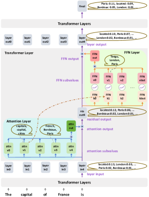
Figure 1: The residual stream of transformers.

Previous studies find FFN subvalues are human-interpretable when projecting into vocabulary space (Geva et al., 2022), but the reason is still unclear. Moreover, the metric for computing the significance of different layers is not unified. Different metrics may draw to different conclusions. For instance, if we compare the ranking of the final prediction in each layer, we can find the ranking drops sharply in shallow layers. So the conclusion is shallow layers are more important. However, if considering the probability of the final prediction, the probability increase mainly exists in deep layers, which indicates deep layers are more useful. Therefore, it is essential to choose a reasonable metric to compute the significance of the layers. Another question is how to evaluate how much one layer is affected by previous layers. It is helpful for understanding how transformers work if these problems are solved.

In this paper, we mainly focus on these problems. By exploring the residual stream, we find subvalues are often human-interpretable when projecting into vocabulary space because the mechanism behind residual connection is an addition function on two vectors’ before-softmax values. Hence, when analyzing the subvalues in vocabulary space, the top words with large before-softmax values can contribute to the final prediction much (Section 3.1). Based on this, we find using log probability increase as metric to compute layers and subvalues’ significance is better than using probability increase, because the curve of log probability increase has a linear monotonically increasing shape (Section 3.2). Moreover, we find how much FFN subvalues are affected by previous layer-level vectors is related to the inner product scores between FFN subkeys and layer-level vectors (Section 3.3).

We utilize our findings to locate the factual knowledge $<$France, capital, Paris$>$ in Section 4. The results are shown in Figure 1. The knowledge is stored separately in deep FFN layers and attention layers. Attention layers store knowledge ”Paris is related to France”, as we find attention subvalues on the ”France” position have concepts about France (e.g. French and Paris) in vocabulary space. FFN layers store knowledge ”Paris is a capital/city”. Our evidence is that we find FFN subvalues with concepts about cities (e.g. London and Paris). Moreover, the most contributing FFN subvalue is activated by an attention subvalue on the ”capital” position. We leverage our analytical method on four models including Baevski-18, GPT2 medium, Llama-7B and Llama-13B. The results can support our analysis.

In conclusion, we explore the residual stream of transformers and explain why the subvalues are human-interpretable in vocabulary space. Also, we use log probability increase as metric and succesfully locate important layers and subvalues. Furthermore, we find FFN subvalues are activated by inner products between previous layer-level vectors and the FFN subkeys. The case study of factual knowledge can prove the correctness of our analysis. To the best of our knowledge, our work is the first to analyze intrinsic interpretability on a large language model with more than 10B parameters. Our methods and findings are helpful for understanding the mechanism of transformers.

2 Background

2.1 The Residual Stream of Transformers

The residual stream of transformers has been explored and proven useful in recent works for mechanistic interpretability (Geva et al., 2022; Olsson et al., 2022). However, previous work focus in either attention layers or FFN layers only. In our study, we focus in both attention layers and FFN layers to analyze the whole residual stream. We take a decoder-only transformer (Baevski & Auli, 2018) as an example. There are 16 layers in this model, and each FFN layer has 4096 neurons. Layer normalization (Ba et al., 2016) is added at the input of each layer. Each FFN layer’s activation function is ReLU. The layer residual stream is:

$$[Lin_{0},Lres_{0},Lout_{0},...,Lres_{15},Lout_{15}]$$ (1)

where $Lin_{i}$ and $Lout_{i}$ denote the layer input and layer output of the $ith$ transformer layer. $Lres_{i}$ is the sum of $ith$ layer input and $ith$ attention layer output (see Figure 1 for more details).

The main characteristic of layer residual stream is that each transformer layer’s input is its previous layer’s output (except the $0th$ layer). For better understanding, we take the sentence ”$<$start$>$ The capital of France is” as an example. On the layer residual stream of the last token, the $ith$ layer output ($i>0$) $Lout^{5}_{i}$ is the sum of its previous layer’s output $Lout^{5}_{i-1}$, current layer’s attention output $ATTN^{5}_{i}$, and current layer’s FFN output $FFN^{5}_{i}$.

$$Lin^{5}_{i}=Lout^{5}_{i-1}$$ (2)

$$Lres^{5}_{i}=Lin^{5}_{i}+ATTN^{5}_{i}$$ (3)

$$Lout^{5}_{i}=Lres^{5}_{i}+FFN^{5}_{i}$$ (4)

where $i$ represents the layer number, and $5$ means the position number of token ”is” ($<$start$>$ is the $0th$ token). Therefore, the final layer output $Lout^{5}_{15}$, which is used for predicting the next word, is computed by the sum of 33 vectors (the $0th$ layer input $Lin^{5}_{0}$, 16 attention outputs, 16 FFN outputs).

In addition to the layer residual stream, the attention outputs and FFN outputs can also be computed by a ”subvalue residual stream”:

$$ATTN^{5}_{i}=attn^{5.0}_{i}+attn^{5.1}_{i}+...+attn^{5.5}_{i}+attn^{b}_{i}$$ (5)

$$FFN^{5}_{i}=ffn^{0}_{i}+ffn^{1}_{i}+...+ffn^{4095}_{i}+ffn^{b}_{i}$$ (6)

Since the example sentence has 6 tokens, each attention layer output can be regarded as the sum of 6 attention subvalues and a bias. Similarly, each FFN layer output can be computed by the sum of 4096 FFN subvalues and a FFN bias. Each attention subvalue is an element-wise multiplication between an attention weight vector and a value vector computed by the layer input (after normalization) and the value matrix $V$. Then the multiplication is multiplied by the output matrix $O$:

$$attn^{5.0}_{i}=(\alpha^{5.0}_{i}(LN(Lin^{0}_{i})V_{i}))O_{i}$$ (7)

where $attn^{5.0}_{i}$ means the $0th$ attention subvalue in layer $i$, queried by the $5th$ token. Its multi-head attention weights $\alpha^{5.0}_{i}$ are computed by the softmax function among the $5th$ query and all positions’ keys on all heads. $V_{i}$ and $O_{i}$ are the value matrix and output matrix. $\alpha^{5.0}_{i}$ is a vector concatenated by attention scores $\alpha^{h}$ on different heads:

$$\alpha=[\alpha^{h1},...,\alpha^{h1},\alpha^{h2},...,\alpha^{h2},...,\alpha^{ht},...,\alpha^{ht}]$$ (8)

where $t$ is the head number. According to Geva et al. (2020), in FFN layers, $ffn^{k}_{i}$ (the $kth$ FFN subvalue in layer $i$) is computed by its coefficient score $m^{k}_{i}$ and the $kth$ vector in FFN’s second fully-connected network $fc2$, where the coefficient score is calculated by the layer normalization of residual output $LN(Lres)$ and the $kth$ vector in FFN’s first fully-connected network $fc1$.

$$m^{k}_{i}=ReLU(LN(Lres_{i})\cdot{fc1}^{k}_{i}+b^{k}_{i})$$ (9)

$$ffn^{k}_{i}=m^{k}_{i}{fc2}^{k}_{i}$$ (10)

Eq.7-8 and Eq.9-10 show the computation of attention subvalues and FFN subvalues respectively. There is a major difference: an attention subvalue is calculated by the element-wise product of two vectors (Eq.7), while a FFN subvalue is calculated by the product of a score and a vector (Eq.10).

2.2 Analyzing Subvalues in Vocabulary Space

Geva et al. (2022) introduce the method of projecting FFN subvalues into vocabulary space. The main idea is to compute the subvalues’ probability distribution on the unembedding matrix $E$. For example, the output distribution $D_{Lout_{15}}$, which is used for predicting the next word, is computed by the final representation $Lout_{15}$ and the unembedding matrix $E$:

$$D_{Lout_{15}}=softmax(E\,Lout_{15})$$

$Lout_{15}$ is the sum of $Lres_{15}$ and $FFN_{15}$. We can compute the distribution of these two vectors to see the probability on all vocabulary words:

$$D_{Lres_{15}}=softmax(E\,Lres_{15})$$

$$D_{FFN_{15}}=softmax(E\,FFN_{15})$$

If the final predicted word’s probability is not high in $D_{Lres_{15}}$ but high in $D_{FFN_{15}}$, we can infer $FFN_{15}$ contains the helpful information about the predicted word. Similarly, we can compute the distribution of a FFN subvalue $ffn_{i}^{k}$ by multiplying the unembedding matrix E:

$$P_{ffn_{15}^{k}}=softmax(E\,ffn_{i}^{k})$$

3 Mechanism Analysis

From previous analysis, the final embedding for prediction is the sum of many layer-level vectors (Eq.1-4), and each layer-level vector is the sum of many subvalues (Eq.5-6). Consequently, a key step toward interpreting the mechanism of transformers is to analyze how the distribution of vectors changes between the residual connections. We explore this in Section 3.1. There are too many layers and subvalues in the models, so how to locate the important layers and subvalues is important. We propose a method in Section 3.2. Moreover, we analyze how much a FFN subvalue is affected by previous layer-level vectors in Section 3.3.

3.1 Distribution Change on the Residual Stream

We explore how the output distribution in the vocabulary space changes when a subvalue $v$ is added on a layer-level vector $x$. With the same unembedding matrix $E$, we project each vector into the vocabulary space $\mathcal{V}\in\mathbb{R}^{B}$ like Section 2.2. For each token $w$, the probabilities are calculated with softmax function:

$$p(w|x)=\frac{exp(e_{w}\cdot x)}{exp(e_{1}\cdot x)+...+exp(e_{B}\cdot x)}$$ (11)

$$p(w|v)=\frac{exp(e_{w}\cdot v)}{exp(e_{1}\cdot v)+...+exp(e_{B}\cdot v)}$$ (12)

$$\begin{split}&p(w|x+v)=\\ &\frac{exp(e_{w}\cdot(x+v))}{exp(e_{1}\cdot(x+v))+...+exp(e_{B}\cdot(x+v))}\end{split}$$ (13)

where $e_{w}$ is the $wth$ row of $E$. If the parameters of the unembedding matrix are shared with the embedding matrix, $e_{w}$ is equal to the embedding of $w$. $e_{w}\cdot x$ is the inner product of $e_{w}$ and $x$. Eq.11-13 reveals the vocabulary distribution of $x+v$ is related to the distributions of $x$ and $v$.

How much distribution change $p(w|x+v)-p(w|x)$ will be caused by vector $v$? Let us term the score $e_{w}\cdot x$ vector $x$’s bs-value (before-softmax value) on token $w$. For $x$ and $v$, a token’s bs-value directly corresponds to the probability and ranking of this token. Bs-values of all vocabulary tokens on vector $x$ are:

$$bs(x)=[bs^{x}_{1},bs^{x}_{2},...,bs^{x}_{w},...,bs^{x}_{B}]$$ (14)

For vector $x$, if $bs^{x}_{w}$ is the largest among all the bs-values, the probability of word $w$ will also be the highest. On every vocabulary token, bs-value $bs^{x+v}_{w}$ is equal to $bs^{x}_{w}+bs^{v}_{w}$, and the probability of each token can be computed by all the bs-values:

$$bs(x+v)=bs(x)+bs(v)$$ (15)

$$p(w|x)=\frac{exp(bs^{x}_{w})}{exp(bs^{x}_{1})+...+exp(bs^{x}_{B})}$$ (16)

The change of bs-values can interpret the mechanism of the distribution change. $bs^{v}_{w}$ is directly added on $bs^{x}_{w}$ to control the probability change. If $bs^{v}_{w}$ is the largest bs-value in vector $v$, vector $v$ will be helpful for increasing the probability of $w$. On the contrary, the probability of the token with the smallest bs-value will decrease. For example, if there are 4 tokens in the vocabulary, and the bs-values of vector $x$ are [1, 2, 3, 4], corresponding to probability [0.03, 0.09, 0.24, 0.64]. Vector $v$ with bs-values [7, 1, 1, 1] will increase the first token’s probability when adding on $x$, changing the bs-values into [8, 3, 4, 5] with probabilities [0.93, 0.01, 0.02, 0.04]. Even though the change of probabilities are non-linear, the change of bs-values are linear. It is mathematically correct that the probability of token with largest bs-value in $v$ will increase in $x+v$, compared with $x$. At the same time, the probability of the token with the smallest bs-value in $v$ will decrease in $x+v$, compared with $x$. Since there are many tokens in the vocabulary, so the top ranking tokens (e.g. top 300) may also have this characteristic.

Our analysis proves that the subvalues can help increase the probability of top tokens when projecting into vocabulary space. If our analysis is correct, we should see human-interpretable concepts on tokens with largest and smallest bs-value tokens. Our experiments in Section 4.1.3 find these tokens, which support our analysis. Geva et al. (2022) also analyzed this distribution change and stated that $p(w|x+v)\propto exp(e_{w}\cdot x)\cdot exp(e_{w}\cdot v)$, but they did not take into consideration other tokens. In our work, we prove that the probability change is also related to other tokens’ bs-values $e_{k}\cdot x$ rather then only $e_{w}\cdot x$ and $e_{w}\cdot v$. We compare our method with theirs in Appendix E.

We can utilize our finding to analyze the roles of coefficient scores in FFN subvalues. A FFN subvalue changes vector $x$ into vector $x+mv$, where $m$ is the coefficient score and $v$ is the fc2 vector (Eq.10). Token $w$’s bs-value is changed from $bs^{x}_{w}$ to $bs^{x}_{w}+m\,bs^{v}_{w}$. Consequently, the role of coefficient score $m$ is to enlarge the distribution change of $v$. If $v$ is helpful for predicting some tokens, larger $m$ can help increase the probabilities of these tokens more in $x+mv$.

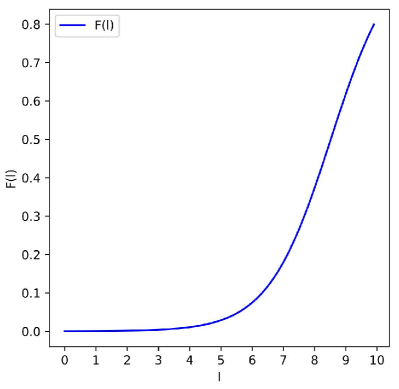
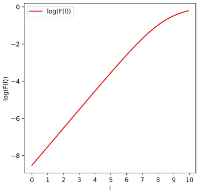
Figure 2: Curves of $F(l)$ and $log(F(l))$.

3.2 Significance Metric for Layers and Subvalues

In this section, we aim to design a method to locate the most important layers and subvalues. A simple method is using probability increase as the significance metric. For instance, we can calculate the probability increase of the $15th$ FFN layer for predicting the final word ”Paris” by $p("Paris"|Lout^{5}_{15})-p("Paris"|Lres^{5}_{15})$. By sorting the probability increase of all layers, the most important layers can be found.

However, is log increase a good metric? A good metric should have the characteristic that the same vector have similar significance scores when adding on different vectors. We add vector $v^{\prime}$ with $bs(v^{\prime})=[0,0,...,bs^{v^{\prime}}_{w},...,0]$ on a changing vector $x$ and analyze the probability change, where $w$ is the final predicted word. Analyzing $bs^{v}_{w}$ is important, because it corresponds to the probability of $w$. The probability of $x+v^{\prime}$ is:

$$\begin{split}&p(w|x+v^{\prime})=\\ &\frac{exp(bs^{x}_{w}+bs^{v^{\prime}}_{w})}{exp(bs^{x}_{w}+bs^{v^{\prime}}_{w})+\sum_{i=1}^{B-\{w\}}{bs^{x}_{i}}}\end{split}$$ (17)

Only the bs-value of token $w$ changes. If we regard $exp(bs^{x}_{w})$ as $A$, $\sum_{i=1}^{B-\{w\}}{bs^{x}_{i}}$ as $C$, $bs^{v^{\prime}}_{w}$ as $l$, Eq.17 is equivalent to:

$$F(l)=\frac{Ae^{l}}{Ae^{l}+C}$$ (18)

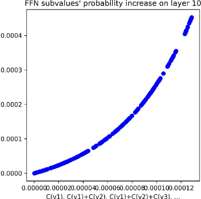
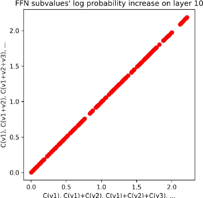
Figure 3: Curves of probability increase and log probability increase of the $10th$ layer FFN subvalues.

On shallow layers, $C$ is usually larger than $A$ since $bs_{w}^{x}$ is usually small. A is different on different layers. The curves of function $F(l)$ and $log(F(l))$ are shown in Figure 2. The same $l$ gains different increase on $F(l)$ because the curve is not linear. Compared with $F(l)$, $log(F(l))$ is like a linear curve, so the log probability increase is similar when adding $v$ on different $x$. So we argue that using log probability increase as significance metric is better than probability increase. The significance metric $C(i)$ of an attention or FFN layer $i$ when predicting word $w$ is:

$$C(ATTN_{i})=log(p(w|Lres_{i}))-log(p(w|Lin_{i}))$$

$$C(FFN_{i})=log(p(w|Lout_{i}))-log(p(w|Lres_{i}))$$ (19)

This metric is also used to compute the significance of an attention or FFN subvalue $v$.

$$C(v_{i})=log(p(w|L_{i}+v_{i}))-log(p(w|L_{i}))$$

where $L_{i}$ is $Lin_{i}$ or $Lres_{i}$ respectively. To verify our analysis, we do an experiment on one layer’s FFN subvalues. We extract all helpful FFN subvalues ($C({v_{i}})$>0), then calculate $C(v1),C(v1+v2),C(v1)+C(v2)+C(v3),...$ and $C(v1),C(v1)+C(v2),C(v1)+C(v2)+C(v3)+...$ . The curves of probability increase and log probability increase are shown in Figure 3. Log probability increase has a linear monotonically increasing shape, while probability increase does not. These results have similar shapes with Figure 2, which match our analysis. Therefore, log probability increase can be used on subvalues because the score is not related to the order. Curves of other layers are similar to Figure 3, shown in Appendix A.

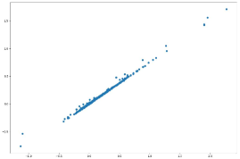
Figure 4: Analysis of layer normalization. x-axis: $Lres_{i}\cdot K^{k}_{i}$, y-axis: $\frac{Lres_{i}\cdot K^{k}_{i}}{V}-\frac{E\lambda_{K}}{V}$.

3.3 How are FFN Subvalues Activated

A FFN subvalue is multiplied by a coefficient score and a fc2 vector (Eq.10). The fc2 vectors are the same in various sentences, while the coefficient scores are different. Therefore, the coefficient score controls how much information of the corresponding fc2 vector is transferred into the final prediction. In this section, we aim to explore how much one FFN subvalue is activated by previous layer-level vectors. A FFN subvalue is activated by this layer’s residual output (Eq.9), and the residual output is the sum of previous layer-level vectors (Eq.2-4). Consequently, each previous layer-level vector affects the coefficient score. If we only consider the activated FFN subvalues (coefficient score>0), Eq.9 is equivalent to:

$$m^{k}_{i}=LN(Lres_{i})\cdot{fc1}^{k}_{i}+b^{k}_{i}$$ (20)

and $Lres_{i}$ is the sum of previous layer vectors:

$$Lres_{i}=Lin_{0}+ATTN_{0}+FFN_{0}+...+ATTN_{i}$$ (21)

Given a FFN subvalue, we aim to explore which vector in Eq.21 plays the largest role for computing its coefficient score. Then we can analyze whether this vector has human-interpretable concepts and understand the mechanism of transformers. If there is no layer normalization in Eq.20, we can compute the inner product between $fc1^{k}_{i}$ and each vector in Eq.21 to see with vector has the largest score. However, does the layer normalization affect the coefficient scores?

$$m^{k}_{i}=(\frac{Lres_{i}-E}{V}LN_{w}+LN_{b})\cdot fc1^{k}_{i}+b^{k}_{i}$$ (22)

$$m^{k}_{i}=\frac{Lres_{i}\cdot K^{k}_{i}}{V}-\frac{E\lambda_{K}}{V}+B^{k}_{i}$$ (23)

Eq.22-23 shows the influence of layer normalization. In Eq.22, $E$ and $V$ are the expectation and variance of $Lres_{i}$. $LN_{w}$ and $LN_{b}$ are learned parameters. In Eq.23, $K^{k}_{i}$ is the element-wise product of $LN_{w}$ and $fc1^{k}_{i}$, $\lambda_{K}$ is the sum of all dimension scores of $K^{k}_{i}$, and $B^{k}_{i}$ is the sum of $LN_{b}\cdot fc1^{k}_{i}$ and $b^{k}_{i}$. For each FFN subvalue, $K^{k}_{i}$ and $B^{k}_{i}$ are the same. We analyze the role of layer normalization by looking at $Lres_{i}\cdot K^{k}_{i}$ and $\frac{Lres_{i}\cdot K^{k}_{i}}{V}-\frac{E\lambda_{K}}{V}$. The relationship is shown in Figure 4. It is approximately a linear shape. The coefficient score is larger when the inner product between $Lres$ and $K^{k}_{i}$ is larger. The expectation $E$ and variance $V$ do not affect the coefficient score much.

Therefore, we can compute how much a layer-level vector in Eq.21 activates a FFN subvalue by computing the inner product between the layer-level vector and $K_{i}^{k}$. We name $K_{i}^{k}$ the FFN subkey.

4 Locating Knowledge in Transformers

In this section, we utilize our findings in Section 3 to locate the factual knowledge $<$France, capital, Paris$>$ in transformer models. We analyze which parameters help the model predict ”Paris” given sentence ”The capital of France is”. We use log probability increase to compute the significance score of each layer and subvalue, and analyze the subvalues in vocabulary space in Section 4.1. We analyze the important FFN subvalues are activated by which vectors in Section 4.2. In Section 4.3 we design a method to analyze why the prediction is ”Paris” rather than ”London” or ”Bordeaux”. In this section, the results and analysis are based on the model in Baevski & Auli (2018) because its activation function in FFN layers is ReLU, which is essential for the experiments in Section 4.1.2. We also apply our method in GPT2 medium (Radford et al., 2019), Llama 7B and 13B (Touvron et al., 2023). On all models we locate the knowledge. The results are shown in Appendix B-D.

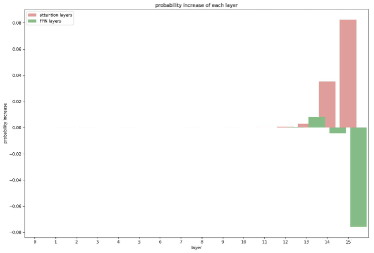
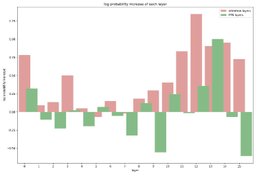
Figure 5: Probability increase (up) and log probability increase (down) of different layers.

4.1 Locating Important Layers and Subvalues

4.1.1 Locating Important Layers

We calculate the probability increase and log probability increase of each attention layer and FFN layer for predicting word ”Paris”. The results are shown in Figure 5. When using probability increase, only 14-15 attention layer have large scores. When applying log probability increase, 11-15 attention layers and 12-13 FFN layers have large scores. In Section 4.1.3 we find interpretable concepts in 11-13 layers, which can support that using log probability increase is more reasonable. Deep layers have larger log probability increase than shallow layers. This indicates the semantic features are stored in deep layers.

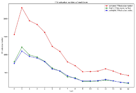
Figure 6: The number of helpful/unhelpful FFN subvalues.

4.1.2 Analyzing Important Subvalues

We aim to explore whether the knowledge is stored in a small number or a large number of subvalues. We analyze the number of activated subvalues (coefficient score>0), helpful subvalues (significance score>0) and unhelpful subvalues (significance score<0) in FFN layers. The results are shown in Figure 6. The numbers of deep layers are smaller than those of shallow layers. But the numbers of helpful and unhelpful subvalues are similar. We also draw the proportion of top 10 subvalues’ sum log probability increase and all the helpful/unhelpful subvalues’ sum log probability increase in Figure 7. In deep layers, the proportion are 40%-45%. This means the top10 subvalues in each deep FFN layer contain much factual knowledge.

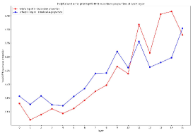
Figure 7: Proportion of top10 subvalues and all subvalues.

Table 1: Important subvalues’ top10 tokens on vocabulary space.

subv	top tokens
$ffn^{1105}_{13}$	Taegu, London, Istanbul, Brussels, Philadelphia, Sleaford, Nagasaki, Calcutta, Kolkata, Baghdad
$ffn^{2038}_{12}$	Batavia, Turin, Jakarta, Harrisburg, Newark, Rome, Toulon, Stoke, Moncton, Colombo
$attn^{4}_{12}$	francs, sur, Bordeaux, Breton, le, Provence, Henri, Petit, Marseille, François
$attn^{4}_{14}$	Provence, Château, Breton, Bordeaux, sur, francs, Philippe, Toulon, Bois, Marseille
$ffn^{2767}_{12}$ (last   tokens)	Argentina, Chilean, Thai, Peruvian, Māori, Colombia, Te, Seoul, Malaysian, Colombian
$attn^{2}_{11}$	capital, capitals, Cities, cities, Strasbourg, Capital, Beijing, Lansing, Astoria, treasury

4.1.3 Analyzing Subvalues in Vocabulary

We analyze the attention subvalues and FFN subvalues in vocabulary space. The top tokens of subvalues with largest log probability increase are shown in Table 1 (the first four rows). In all these subvalues, ”Paris” ranks in top 200. FFN subvalues $ffn_{13}^{1105}$ and $ffn_{12}^{2038}$ contain different cities. Attention subvalues $attn_{12}^{4}$ and $attn_{14}^{4}$ have concepts related to ”France”. Also, we find the tokens with smallest bs-values on an unhelpful FFN subvalue $ffn_{12}^{2767}$ have concepts related to different cities (the $5th$ row in Table 1). These results support our previous analysis in Section 3.1.

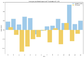
Figure 8: Inner products between the subkey of $ffn_{13}^{1105}$ and each previous layer-level vector.

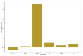
Figure 9: Inner products between the subkey of $ffn_{13}^{1105}$ and the $11th$ attention layer subvalues.

4.2 Vectors Activating Important Subvalues

In this section, we aim to analyze which vectors are helpful for activating the most important FFN subvalue $ffn_{13}^{1105}$. We compute the inner products of each attention and FFN layer vector and the subkey of $ffn_{13}^{1105}$. The inner products are shown in Figure 8. The $11th$ attention layer has the largest score. Then we compute the inner products between the subkey of $ffn_{13}^{1105}$ and the $11th$ attention layer’s subvalues in Figure 9. The $2th$ subvalue has the largest score. By analyzing it in vocabulary space (the last row in Table 1), we find the $2th$ subvalue’s concepts are related to ”city”.

Based on the results and analysis, we have located the factual knowledge of $<$France, capital, Paris$>$ in the model. The knowledge of ”Paris is a capital/city” is stored in deep FFN subvalues, which are activated by the attention subvalues related to ”capital/city”. The knowledge of ”Paris is related to France” is stored in value-output matrices in deep attention layers.

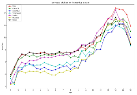
Figure 10: Bs-values of different cities on the residual stream.

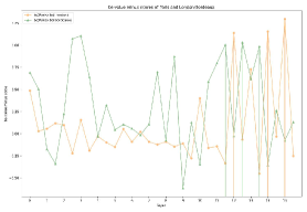
Figure 11: Bs-value minus scores between ”Paris” and ”London”/”Bordeaux”. 0, 1, …, 15 corresponds to attention layers. 0.5, 1.5, …, 15.5 corresponds to FFN layers.

4.3 Comparison to Different Cities

What we want to explore more are the parameters help distinguish ”Paris” from other cities (such as ”London”, ”Brussels”, ”Marseille”, ”Bordeaux”). We draw the bs-values of the cities on the residual stream in Figure 10. By comparing the bs-values, we can see which city has the largest probability in different layers. And we can also find the important layers for distinguishing different cities by computing the bs-value minus scores. We draw the bs-value minus scores between ”Paris” and ”London”/”Bordeaux” in Figure 11. We can find that the largest bs-value minus change $bs_{Paris}-bs_{London}$ between ”Paris” and ”London” are in attention layers, while the largest bs-value minus change between ”Paris” and ”Bordeaux” are in FFN layers. These results are similar to our analysis. ”London” is not related to ”France” much, so attention layers can help distinguish ”Paris” and ”London”. Compared with ”Paris”, ”Bordeaux” has smaller bs-value scores in FFN subvalues related to ”capital”. Therefore, FFN layers help distinguish ”Paris” and ”Bordeaux”.

5 Discussion

In this section, we aim to discuss the roles of subvalues. A subvalue is not only working as a ”value” to directly increase the probability of the final prediction, but also a ”query” to activate higher subvalues.

Working as ”value”. The subvalues with large log probability increase are mainly working as ”values”, which can contribute to the final prediction of ”Paris” directly. In this situation, ”Paris” has a large bs-value in these FFN subvalues. A FFN subvalue has three abilities when working as ”value”. First, it can increase the probability of tokens with very large bs-values (e.g. $ffn_{13}^{1105}$ and $attn_{12}^{4}$). Second, it can decrease the probability of tokens having very small bs-values (e.g. $ffn_{12}^{2707}$). At the same time, it can help distinguish two tokens if a token’s bs-value is large and another token’s bs-value is small. Note that a FFN subvalue is computed by the product of a coefficient score and a fc2 vector. The fc2 vectors are the same in every sentence. Hence, the ability of one fc2 vector is similar in different cases.

Working as ”query”. When working as ”query”, a subvalue may not contribute to the final prediction directly. It works by activating other useful subvalues (e.g. $attn_{11}^{2}$). In Section 4.2, we only analyze the $11th$ attention layer with the largest inner product. While the $10th$ FFN layer’s inner product is also larger than 0. Therefore, there are also FFN subvalues helpful for activating $ffn_{13}^{1105}$.

Our analysis can explain some phenomenons. The methods proposed by Meng et al. (2022b) hypothesize the model should modify medium and deep FFN layers containing knowledge during fine-tuning. However, Hase et al. (2023) find the model tends to modify the parameters in shallow FFN layers. Maybe the reason of this phenomenon is the model modifies the ”queries” instead of the ”values”. A ”query” in shallow layers affects many ”values” in deep layers, so it is efficient for the model to modify the ”queries”.

6 Related Work

Many previous studies have explored the mechanism of transformers. Geva et al. (2020) demonstrate that FFN layers can be regarded as key-value memories. Based on this, Dai et al. (2021) hypothesize that factual knowledge is stored in FFN layers, and evaluate the contribution scores of each FFN subvalue using integrated gradients. Geva et al. (2022) explain model parameters by computing their distribution over the vocabulary, and find the subvalues in the FFN modules are often interpretable. By analyzing the residual stream, Elhage et al. (2021) and Olsson et al. (2022) find the relationship between in-context learning and induction heads, and Dar et al. (2022) find that transformers can be interpreted by projecting all parameters into the embedding space. Another common method for exploring interpretability is based on causal mediation analysis (Meng et al., 2022a; Geva et al., 2023), but Hase et al. (2023) argue that location conclusions from these methods are not the parameters they actually modify.

A corresponding field is modifying a model’s knowledge. Yao et al. (2023) discuss four main methods: memory-based model (Mitchell et al., 2022), adding new parameters (Huang et al., 2023), meta learning (De Cao et al., 2021) and locate-then-edit (Dai et al., 2021; Meng et al., 2022a). Our research helps find knowledge locations, so it may be helpful for the locate-then-edit method.

7 Conclusion

In this paper, we explore the mechanism behind the residual stream of transformers and locate factual knowledge in a transformer model. We find why subvalues have human-interpretable concepts in vocabulary space. The reason is the addition function on before-softmax values among residual connections can enlarge the probabilities related to top vocabulary tokens. Based on this analysis, we find using log probability increase as significance metric can help find the important layers and subvalues. Furthermore, we prove that the FFN subvalues are activated by previous layers through the inner products between the FFN subkeys and the previous layer-level vectors. We utilize our analysis and find that factual knowledge $<$France, capital, Paris$>$ is stored in deep FFN layers and deep attention value-output matrices. Specifically, the FFN subvalues are activated by attention subvalues related to ”capital/city”. We conduct experiments on small models and large language models. These results can prove that our analysis about the mechanisms is correct. Overall, our work is helpful for understanding the mechanism of transformers.

8 Broader Impact

This paper presents work whose goal is to advance the field of interpreting large language models. There are many potential societal consequences of our work, none which we feel must be specifically highlighted here.

Appendix A Significance Scores of FFN Subvalues in Different Layers

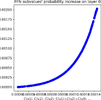
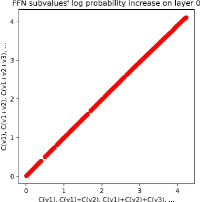
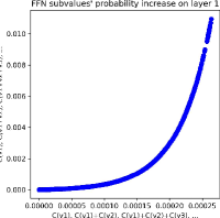
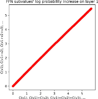
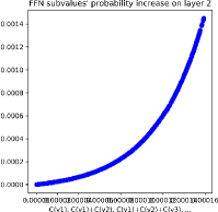
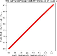
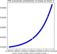
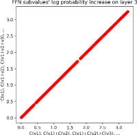
Figure 12: Curves of FFN subvalues’ significance scores in 0-3 layers. left: probability increase. right: log probability increase.

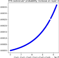
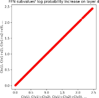
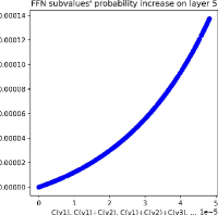
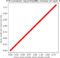
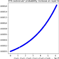
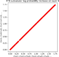
Figure 13: Curves of FFN subvalues’ significance scores in 4-7 layers. left: probability increase. right: log probability increase.

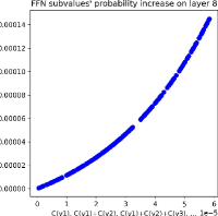
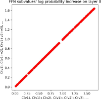
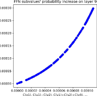
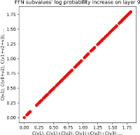
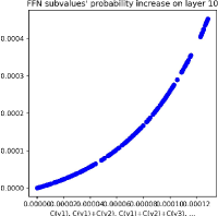
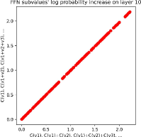
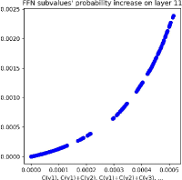
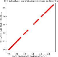
Figure 14: Curves of FFN subvalues’ significance scores in 8-11 layers. left: probability increase. right: log probability increase.

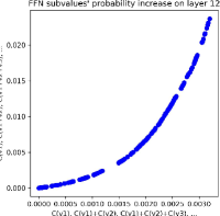
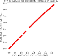
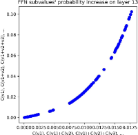
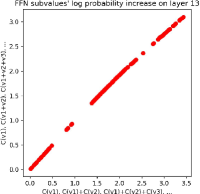
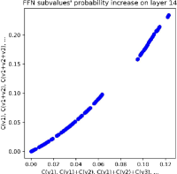
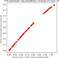
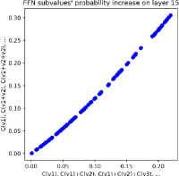
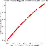
Figure 15: Curves of FFN subvalues’ significance scores in 12-15 layers. left: probability increase. right: log probability increase.

Appendix B Significance of Different Layers in GPT2 Medium for Predicting ”Paris”

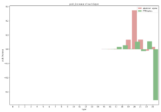
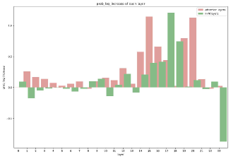
Figure 16: Significance of layers in GPT2 Medium on different metrics. left: probability increase. right: log probability increase.

Figure 16 shows the probability increase and log probability increase of each layer in GPT2 medium. The input sentence is ”The capital of France is” and the prediction is ”Paris”. Figure 16 has a similar trend with Figure 5. When taking probability increase as significance metric, only the $20th$ attention layer has a large score. When using log probability increase, many deep layers (15-20) have large scores. In Appendix C, we find interpretable results on these layers. Therefore, using log probability increase as significance metric is better than using probability increase. The results can support our analysis in Section 3.2.

Appendix C Analysis on Different Cases on Baevski-18 and GPT2 Medium

According to Petroni et al. (2019), language models can learn 1-1 relationships well, such as $<$country, capital, city$>$ and $<$city, located-in, country$>$. Therefore, we apply our methods on these relationships. We use ”The capital of X is” and ”Y is located in the country of” as prompts, where X and Y are names of countries and cities respectively. We analyze the attention and FFN subvalues with large log probability increase for predicting the correct word. We analyze these sentences on Baevski-18 Baevski & Auli (2018) and GPT2 Medium (Radford et al., 2019). The results are shown in Table 2.

Table 2: Important subvalues’ top10 tokens in vocabulary space. ”rank”: the prediction’s ranking in vocabulary space. ”increase”: the log probability increase of each subvalue.

prompt -$>$ output	model	subv	rank	increase	top10 tokens in vocabulary space
The capital of UK is London	Baevski	$attn_{13}^{4}$	1	0.6683	UK, London, Peel, Britons, GB, British, Surrey, Britain, Blur, Thames
The capital of UK is London	Baevski	$ffn_{13}^{1105}$	1	0.6490	Taegu, London, Istanbul, Brussels, Philadelphia, Sleaford, Nagasaki, Calcutta, Kolkata, Baghdads
The capital of Germany is Berlin	Baevski	$attn_{12}^{4}$	27	1.4394	Weimar, Lützow, Göring, Deutschland, Der, Kriegsmarine, Hindenburg, Nazis, Junkers, Fritz
The capital of Germany is Berlin	Baevski	$ffn_{14}^{3391}$	176	0.4297	Turin, Helsinki, Lisbon, Jakarta, Sarajevo, Prague, Monaco, Arnhem, Kolkata, Hiroshima
The capital of France is Paris	GPT2 medium	$attn_{20}^{4}$	6	1.0959	French, French, France, France, Hollande, Frenchman, Paris, french, Paris, Marse
The capital of France is Paris	GPT2 medium	$ffn_{17}^{2282}$	78	0.6105	ère, François, Quebec, Franç, É, é, French, ée, franc, è
The capital of France is Paris	GPT2 medium	$ffn_{20}^{1978}$	51	0.1432	Pittsburgh, Atlanta, Montreal, Chicago, Baltimore, Toronto, Seattle, Philadelphia, Manila, Cincinnati
The capital of Germany is Berlin	GPT2 medium	$attn_{15}^{4}$	7	0.9242	Merkel, Bundesliga, Munich, German, German, Bundes, Mü, Berlin, Germany, Germany
The capital of Germany is Berlin	GPT2 medium	$ffn_{17}^{1041}$	10	1.0923	Munich, Bundes, Bundesliga, Reich, Bav, Merkel, Frankfurt, Friedrich, Germany, Cologne
The capital of Germany is Berlin	GPT2 medium	$ffn_{20}^{1978}$	51	0.1432	Pittsburgh, Atlanta, Montreal, Chicago, Baltimore, Toronto, Seattle, Philadelphia, Manila, Cincinnati
Paris is located in the country of France	Baevski	$attn_{12}^{1}$	3	1.2747	Paris, Louvre, francs, France, Philippe, Bastille, Arc, French, Henri, sur
Paris is located in the country of France	Baevski	$ffn_{12}^{3202}$	18	0.2512	Denmark, Netherlands, Germany, Norway, Belgium, Luxembourg, Czech, Sweden, Tonga, Russia
Paris is located in the country of France	GPT2 medium	$attn_{16}^{1}$	4	1.1567	Paris, Paris, France, French, France, French, Brussels, Hollande, François, Luxembourg
Paris is located in the country of France	GPT2 medium	$ffn_{16}^{1576}$	36	0.4953	Australia, Philippines, Spain, Netherlands, Australia, countries, States, Ireland, Germany, Canada
Paris is located in the country of France	GPT2 medium	$ffn_{17}^{2282}$	27	0.6044	ère, François, Quebec, Franç, É, é, French, ée, franc, ’è’

All the important subvalues have human-interpretable concepts. When predicting the cities, different sentences tend to activate similar FFN subvalues (e.g. $ffn_{13}^{1105}$ in Baevski and $ffn_{20}^{2978}$ in GPT2 medium). The fc2 vectors are the same in different cases, so the knowledge related to one concept can be stored in a FFN subvalue. In GPT2 medium, we not only find FFN subvalues storing ”city”, but also find those storing concepts about ”France” ($ffn_{17}^{2282}$) and ”German” ($ffn_{17}^{1041}$). We hypothesize this is because GPT2 medium has more layers than Baevski and have more parameters to store knowledge. When predicting the countries, we find FFN subvalues related to countries ($ffn_{12}^{3202}$ in Baevski and $ffn_{16}^{1576}$ in GPT2 medium). In all subvalues, the ranking of the final prediction is in top200. This supports our analysis in Section 3.1. We also find that the rankings in attention subvalues are smaller than those in FFN subvalues. This may indicate value-output matrices in attention layers are able to gain more information than FFN layers, because fc2 vectors in FFN layers are fixed.

Appendix D Analysis on Llama 7B and Llama 13B

We leverage our method on Llama 7B and Llama 13B (Touvron et al., 2023) for sentence ”The capital of France is”, shown in Table 3. The correct word ”Paris” have high rankings on located attention and FFN subvalues, and the top words also have related concepts in vocabulary space. Different from Baevski-18 and GPT2 medium, we also find important attention subvalues on the last position in Llama 7B ($attn_{25}^{5}$) and Llama 13B $attn_{27}^{5}$. We hypothesize this is because the Llama models have already gained enough knowledge in medium layers and have passed enough knowledge into the last token. Since the models have much more parameters and neurons in each layer, they can gain the knowledge earlier.

Table 3: Important subvalues’ top10 tokens in vocabulary space on Llama 7B and 13B.

prompt -$>$ output	model	subv	rank	increase	top10 tokens in vocabulary space
The capital of France is Paris	Llama 7B	$attn_{23}^{4}$	3	0.8575	France, French, Paris, Frankreich, französischen, französ, rench
The capital of France is Paris	Llama 7B	$attn_{25}^{5}$	0	0.6097	Paris, French, France, Madrid, Lond, London, Toul
The capital of France is Paris	Llama 7B	$attn_{21}^{4}$	0	0.5452	Paris, French, France, Frankreich, französ, Monsieur]
The capital of France is Paris	Llama 7B	$ffn_{19}^{5771}$	17	0.2513	city, cities, mayor, città, cidade, metropol, City, meg, Mayor
The capital of France is Paris	Llama 7B	$ffn_{17}^{9162}$	0	0.2390	France, French, Paris, französischen, Frankreich, französ, français
The capital of France is Paris	Llama 7B	$ffn_{17}^{4443}$	47	0.1706	London, Bonn, Stockholm, Tokyo, Lond, Dublin, Berlin, Lis, Rome, Lima
The capital of France is Paris	Llama 13B	$attn_{22}^{4}$	1	1.4302	France, Paris, French, Frankreich, französischen, rench, París
The capital of France is Paris	Llama 13B	$attn_{27}^{5}$	0	1.3347	Paris, France, French, französischen, Parse, Frankreich, rench
The capital of France is Paris	Llama 13B	$attn_{21}^{4}$	0	0.9958	Paris, France, French, Marse, Frankreich, Toul
The capital of France is Paris	Llama 13B	$ffn_{26}^{11183}$	4	0.4130	London, Chicago, Lond, Tokyo, Paris, Toronto, Moscow, Sydney, Madrid, Berlin
The capital of France is Paris	Llama 13B	$ffn_{23}^{7967}$	13	0.1870	Washington, Moscow, Tokyo, London, Ott, Madrid, Berlin, Budapest, Sac, Lond
The capital of France is Paris	Llama 13B	$ffn_{18}^{9798}$	0	0.1558	Paris, French, France, Frankreich, Seine, français, perf

A potential advantage of our method is the efficiency to locate the important subvalues on large language models. On Llama 13B, the time (16 CPUs, 0 GPU) for computing the significance scores and the subvalues’ top tokens in vocabulary space is less than 1 minute for a sentence (not including the time of storing vectors and loading models). Therefore, our method can be utilized to analyze other cases quickly, in order to unveil the mystery of transformers.

Appendix E Comparison of Locating Methods

In this section, we compare our method with Geva et al. (2022) for locating important FFN subvalues. They utilize the product of the coefficient score and the subvalue’s norm as significance score. While we take the log probability increase as significance score for each FFN subvalue. We extract the top4 FFN subvalues using the two methods on sentence ”The capital of France is” in Llama 7B. We compute log probability increase, coefficient score, subvalue norm, and correct token ranking for comparison. The results are shown in Table 4.

Table 4: Important subvalues’ top tokens in vocabulary space on Llama 7B.

subv	increase	rank	coeff	norm	coeff*norm	top10 tokens in vocabulary space
$ffn_{19}^{5771}$	0.2513	17	-4.86	7.25	35.30	city, cities, mayor, city, città, cidade, metropol, City, meg, Mayor
$ffn_{17}^{9162}$	0.2390	3	-2.54	4.13	10.53	France, French, Paris, französischen, Frankreich, französ, français
$ffn_{21}^{7178}$	0.2001	16	4.59	6.29	28.95	Gene, Buch, Rome, Nancy, Lyon, Florence, Wars, Bru, Ath, Gen
$ffn_{27}^{4668}$	0.1979	7	-3.16	3.47	11.01	Jean, French, Pierre, France, Paris, Monsieur, Jacques
$ffn_{31}^{5554}$	0.1450	16175	36.52	35.98	1314.3	Kontrola, lär, anzen, ánico, ensoort, Hinweis, oreign
$ffn_{31}^{8965}$	0.0019	3180	33.76	33.13	1119.1	prüfe, consultato, (, ?), %., oo, measured, :], :+
$ffn_{31}^{10993}$	-0.005	22328	29.58	27.37	809.8	Genomsnitt, Normdatei, regnig, Normdaten, Kontrola, ungsseite, Audiod
$ffn_{31}^{566}$	-0.016	21698	-28.12	26.62	748.8	iből, consultato, formatt, orsz, DECLARE

The first 4 rows are FFN subvalues located by our method using log probability increase. The last 4 rows are located using the product of coefficient score and subvalue norm. Our method has better interpretable concepts in vocabulary space. According to the analysis in Section 3.1, the final predicted word should have top ranking when projecting the import FFN subvalues into vocabulary space. Our method can locate these FFN subvalues on different layers. The other method can only locate the subvalues on the same layer ($31th$). Maybe this is because the norm of subvalues in layer 31 are larger than other layers. We find the coefficient scores in important subvalues are not usually larger than 0 (e.g. $ffn_{19}^{5771}$). In this situation, the coefficient scores help reverse the last tokens into top tokens. There are 32,000 tokens in vocabulary space. ”Paris” ranks 31,983 in the origin fc2 vector $fc2_{19}^{5771}$. When the coefficient score is smaller than 0, the tokens with smallest bs-values (smaller than 0) change into the tokens with largest bs-values. Again, the results support our analysis about bs-values.

References

- Alex et al. (2021) Alex, N., Lifland, E., Tunstall, L., Thakur, A., Maham, P., Riedel, C. J., Hine, E., Ashurst, C., Sedille, P., Carlier, A., et al. Raft: A real-world few-shot text classification benchmark. arXiv preprint arXiv:2109.14076, 2021.
- Ba et al. (2016) Ba, J. L., Kiros, J. R., and Hinton, G. E. Layer normalization. arXiv preprint arXiv:1607.06450, 2016.
- Baevski & Auli (2018) Baevski, A. and Auli, M. Adaptive input representations for neural language modeling. arXiv preprint arXiv:1809.10853, 2018.
- Brown et al. (2020) Brown, T., Mann, B., Ryder, N., Subbiah, M., Kaplan, J. D., Dhariwal, P., Neelakantan, A., Shyam, P., Sastry, G., Askell, A., et al. Language models are few-shot learners. Advances in neural information processing systems, 33:1877–1901, 2020.
- Chowdhery et al. (2022) Chowdhery, A., Narang, S., Devlin, J., Bosma, M., Mishra, G., Roberts, A., Barham, P., Chung, H. W., Sutton, C., Gehrmann, S., et al. Palm: Scaling language modeling with pathways. arXiv preprint arXiv:2204.02311, 2022.
- Dai et al. (2021) Dai, D., Dong, L., Hao, Y., Sui, Z., Chang, B., and Wei, F. Knowledge neurons in pretrained transformers. arXiv preprint arXiv:2104.08696, 2021.
- Dar et al. (2022) Dar, G., Geva, M., Gupta, A., and Berant, J. Analyzing transformers in embedding space. arXiv preprint arXiv:2209.02535, 2022.
- De Cao et al. (2021) De Cao, N., Aziz, W., and Titov, I. Editing factual knowledge in language models. arXiv preprint arXiv:2104.08164, 2021.
- Elhage et al. (2021) Elhage, N., Nanda, N., Olsson, C., Henighan, T., Joseph, N., Mann, B., Askell, A., Bai, Y., Chen, A., Conerly, T., et al. A mathematical framework for transformer circuits. Transformer Circuits Thread, 1, 2021.
- Geva et al. (2020) Geva, M., Schuster, R., Berant, J., and Levy, O. Transformer feed-forward layers are key-value memories. arXiv preprint arXiv:2012.14913, 2020.
- Geva et al. (2022) Geva, M., Caciularu, A., Wang, K. R., and Goldberg, Y. Transformer feed-forward layers build predictions by promoting concepts in the vocabulary space. arXiv preprint arXiv:2203.14680, 2022.
- Geva et al. (2023) Geva, M., Bastings, J., Filippova, K., and Globerson, A. Dissecting recall of factual associations in auto-regressive language models. arXiv preprint arXiv:2304.14767, 2023.
- Hase et al. (2023) Hase, P., Bansal, M., Kim, B., and Ghandeharioun, A. Does localization inform editing? surprising differences in causality-based localization vs. knowledge editing in language models. arXiv preprint arXiv:2301.04213, 2023.
- Huang et al. (2023) Huang, Z., Shen, Y., Zhang, X., Zhou, J., Rong, W., and Xiong, Z. Transformer-patcher: One mistake worth one neuron. arXiv preprint arXiv:2301.09785, 2023.
- Ma et al. (2023) Ma, Y., Cao, Y., Hong, Y., and Sun, A. Large language model is not a good few-shot information extractor, but a good reranker for hard samples! arXiv preprint arXiv:2303.08559, 2023.
- Meng et al. (2022a) Meng, K., Bau, D., Andonian, A., and Belinkov, Y. Locating and editing factual associations in gpt. Advances in Neural Information Processing Systems, 35:17359–17372, 2022a.
- Meng et al. (2022b) Meng, K., Sharma, A. S., Andonian, A., Belinkov, Y., and Bau, D. Mass-editing memory in a transformer. arXiv preprint arXiv:2210.07229, 2022b.
- Mitchell et al. (2022) Mitchell, E., Lin, C., Bosselut, A., Manning, C. D., and Finn, C. Memory-based model editing at scale. In International Conference on Machine Learning, pp. 15817–15831. PMLR, 2022.
- Olsson et al. (2022) Olsson, C., Elhage, N., Nanda, N., Joseph, N., DasSarma, N., Henighan, T., Mann, B., Askell, A., Bai, Y., Chen, A., et al. In-context learning and induction heads. arXiv preprint arXiv:2209.11895, 2022.
- Ouyang et al. (2022) Ouyang, L., Wu, J., Jiang, X., Almeida, D., Wainwright, C., Mishkin, P., Zhang, C., Agarwal, S., Slama, K., Ray, A., et al. Training language models to follow instructions with human feedback. Advances in Neural Information Processing Systems, 35:27730–27744, 2022.
- Petroni et al. (2019) Petroni, F., Rocktäschel, T., Lewis, P., Bakhtin, A., Wu, Y., Miller, A. H., and Riedel, S. Language models as knowledge bases? arXiv preprint arXiv:1909.01066, 2019.
- Radford et al. (2019) Radford, A., Wu, J., Child, R., Luan, D., Amodei, D., Sutskever, I., et al. Language models are unsupervised multitask learners. OpenAI blog, 1(8):9, 2019.
- Räuker et al. (2023) Räuker, T., Ho, A., Casper, S., and Hadfield-Menell, D. Toward transparent ai: A survey on interpreting the inner structures of deep neural networks. In 2023 IEEE Conference on Secure and Trustworthy Machine Learning (SaTML), pp. 464–483. IEEE, 2023.
- Touvron et al. (2023) Touvron, H., Lavril, T., Izacard, G., Martinet, X., Lachaux, M.-A., Lacroix, T., Rozière, B., Goyal, N., Hambro, E., Azhar, F., et al. Llama: Open and efficient foundation language models. arXiv preprint arXiv:2302.13971, 2023.
- Vaswani et al. (2017) Vaswani, A., Shazeer, N., Parmar, N., Uszkoreit, J., Jones, L., Gomez, A. N., Kaiser, Ł., and Polosukhin, I. Attention is all you need. Advances in neural information processing systems, 30, 2017.
- Yao et al. (2023) Yao, Y., Wang, P., Tian, B., Cheng, S., Li, Z., Deng, S., Chen, H., and Zhang, N. Editing large language models: Problems, methods, and opportunities. arXiv preprint arXiv:2305.13172, 2023.
- Zhang et al. (2023) Zhang, T., Ladhak, F., Durmus, E., Liang, P., McKeown, K., and Hashimoto, T. B. Benchmarking large language models for news summarization. arXiv preprint arXiv:2301.13848, 2023.