Congestions and Spectral Transition in Time-Lagged Correlations of Motorway Traffic
Abstract. The congestion of a motorway section is propagated to its neighbouring sections, leading to correlations. The resulting correlation matrix encodes the information on congestion. Here, we study symmetrized time-lagged correlations and show how their spectral properties reveal congestion durations. We carry out an empirical analysis and find a transition behavior for the dominant eigenvalue as function of the time lag. Furthermore, we set up a numerical simulation model for indicator time series of traffic phases as well as a simplified model that we treat analytically. We consider various scenarios. Our results reveal a nonlinear relation between the spectral transition and the congestion duration. In our simplified model, we derive this relation analytically.
Keywords: time-lagged correlation, spectral transition, congestion duration, traffic network, complex system
1 Introduction
Many factors trigger traffic congestions, such as traffic accidents, bottlenecks, commute flows, special events, bad weather etc. A report of the U. S. Federal Highway Administration reveals that the duration of weekday peak-period congestion increases from 4.5 hours per day in 1982 to 7.0 hours per day in 2003 for the largest US cities [1]. In 2022, the drivers in London spent an average of 156 hours in traffic delays [2]. Inrix 2022 Global Traffic Scorecard manifests that drivers in USA, UK and Germany lost, on average, dozens of hours in 2022, leading to considerable expenses in time and fuel costs [2]. Nowadays, a wealth of data is available that awaits statistical analysis. Here we focus on the interplay between correlations and congestion durations.
A traffic network as a whole can be viewed as a complex system partly similar to others, e.g., financial markets [3], human brains [4], power systems [5], global climate [6], and so on [7]. A traffic network comprises many constituents, e.g., road sections coupled via the motion of vehicles [8, 9, 10], resulting in real-time traffic flows and velocities. The time series of traffic flows or velocities exhibit non-stationary characteristics and non-Markovian features at a certain time scale [11, 12, 13], distinguished by different traveling behaviors on workdays and holidays, seasonality, the presence of trucks, road construction and so on. The traffic flows also feature anti-persistent behavior, which has an impact on the congestion duration at different time scales [12]. Due to the propagation of traffic flows [14], all its features generate correlations between the sections in the networks. There are spatial [15] and temporal [11] correlations. Spectral analyses of correlation matrices reveal the emergence of collective behavior [16] and subdominant collective behavior [17] in large traffic networks. Statistical responses of the velocities and flows to congestions [18, 19] have also been studied.
The motion of vehicles among different road sections consumes time, giving rise to a time delay in the propagation of congestion effects and thus to non-Markovian statistics. Therefore, it is very interesting to explore time-lagged correlations. The time-lagged correlations [7] are widely used in many fields, including traffic. For motorway traffic, they have been used for the predication of traffic flows or velocities [20, 21], the identification and prediction of traffic phases [22, 23], for understanding the velocity change over space and time [24], estimating the congestion propagation speed between neighbouring sections [25], studying the effects of upstream and downstream traffic on the section between them [26, 27], spectral analyses on oscillation patterns of traffic data [28], and correlation analyses for different motorway lanes [29, 30], etc. The above studies, however, are restricted to a pair of motorway sections. To analyze a motorway network as a whole that comprises many sections, the investigation of the entire corresponding correlation matrix is called for.
Our previous studies [11, 16, 15, 17] of large correlation matrices for traffic networks were restricted to equal-time correlations. Here, we extend this to time-lagged correlations. We dissect the empirical correlation matrices and study the statistics of the spectra. We identify spectral transitions and show how they relate to congestion durations. We perform empirical analyses and, moreover, introduce an indicator model which we analyze numerically and which we solve analytically in a simplified version.
The paper is organized as follows. In section 2, we describe our traffic data, sketch the methods and show empirical results. In section 3, we set up an indicator model and perform simulations to explore the relation between congestion durations and transitions of eigenvalues as function of time lag. We then analytically solve a simplified version of the model in section 4. We draw our conclusions in section 5.
2 Spectral transitions in time-lagged correlations in the presence of congestions
We describe the used traffic data in section 2.1. We introduce symmetrized original and extended correlation matrices in section 2.2. Furthermore, we display the evolution behavior of their eigenvalues for two motorway networks in section 2.3.
2.1 Data description
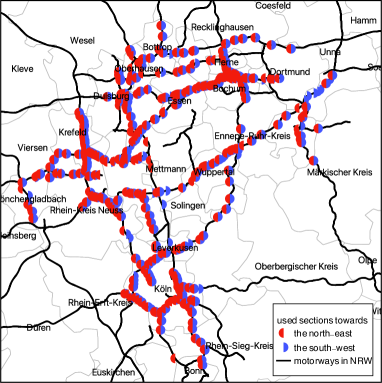
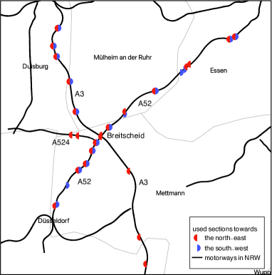
We use the traffic data collected by inductive loop detectors on 679 motorway sections in the Rhine-Ruhr metropolitan region and on 42 motorway sections around Breitscheid, all in North Rhine-Westphalia (NRW), Germany, see figure 1. The data with a resolution of one minute contains the information on time, traffic flow (i.e., the number of vehicles passing a detector per unit time) and velocity for every lane of each section.
As described in references [16, 11, 17], a motorway network exhibits different behavior on workdays and on holidays, resulting in different correlation structures between motorway sections. Here, we only use the traffic data on workdays, and focus on the afternoon rush hours (15:00–20:00), when the commute flows are more likely to produce traffic congestion. The fundamental diagram in traffic theory [31] implies that a specific traffic flow value may correspond to free as well as to congested flow, while a specific velocity value must correspond to either free or congested flow. In the latter case, it is easier to distinguish different traffic phases. Therefore, we use velocity time series to work out the empirical correlations between motorway sections.
Missing values in a data matrix will influence the spectral decomposition of the corresponding correlation matrix. To avoid this, we fill the missing values of each time series by linear interpolation of the nearest non-zero values. At the beginning or at the end of a time series, we replace the missing values with the subsequent or previous values, respectively.
2.2 Time-lagged correlation matrices
A time series of velocities in section with length is denoted by . There are such time series , , which we order in a rectangular data matrix
| (1) |
The time series of section is the -th row of , where the superscript , anticipating later usage, refers to the original data. Here for the Rhine-Ruhr metropolitan region and for the region around Breitscheid. We introduce two projection matrices
| (6) |
where is a identity matrix, and , and are , and zero matrices, respectively. With equation (6), the time series from time to in can be written as the matrix and from to in as the matrix .
For a time series from time to time , mean value and standard deviation read
| (7) |
respectively. We normalize each time series to zero mean and unit standard deviation by
| (8) |
and introduce and as the normalized data matrices of and , respectively. This yields a time-lagged correlation matrix with time lag ,
| (9) |
where indicates the transpose, such that
| (10) |
is the time-lagged correlation coefficient between sections and . We notice that the sum runs from to . Consider the motorway sections in a data matrix labeled by numbers in an ascending order. For , in equation (10) measures the time-lagged correlation between sections and , where the velocity in section lags behind the one in section at time . Considering the velocity in section at an earlier time , the time lag requires the corresponding velocity on section occurring also at an earlier time . Therefore we can reformulate as
| (11) |
where now the sum runs from to . Equation (11) can be regarded as the time-led correlation coefficient between sections and with reference time . For , either as in equation (10) or as in equation (11) gives the autocorrelation of section or . When , the correlation matrix reduces to the standard equal-time Pearson correlation matrix which is symmetric and positive semidefinite with real and positive eigenvalues. When , is asymmetric, leading to complex eigenvalues. The symmetrized time-lagged correlation matrix
| (12) |
however has real eigenvalues which can be negative. The elements
| (13) |
of the matrix is the average of the time-lagged correlation and the time-lead correlation, and the scenarios and are not distinguished.

Equation (9) is widely used for calculating correlation matrix with a time lag. A drawback of this equation is that the length of time series for calculation becomes ever shorter with increasing . This might give rise to poor statistics for very large . We thus make the length of the time series used independent of by extending the interval between and to the interval between and for the lagged time series. Thus, the data outside the initial time series between and are included, as sketched in figure 2. Here is a extended data matrix, where superscript , anticipating the later usage, refers to the extended data. Accordingly, and are two projecting matrices. We use and to represent the normalized data matrices of and . In contrast to the lagged time series, the leading time series is fixed from and for any . We refer to the correlations between the leading and lagged time series as extended correlations. The extended time-lagged correlation matrix is
| (14) |
with the elements given by
| (15) |
or
| (16) |
As in equation (12), the symmetrization of this correlation matrix results in , of which each element is the average of the time-lagged correlation and the time-led correlation.
2.3 Spectral properties as functions of the time lag
To study the spectra, we diagonalize the symmetrized, hence real-symmetric, matrices,
| (17) |
where the diagonal matrix contains the real eigenvalues of . All eigenvalues are ranked in an ascending order, such that and are the smallest and the largest eigenvalues, respectively. The -th column of the orthogonal matrix is the eigenvector to the eigenvalue . The non-symmetrized matrices are real, but not symmetric for . Thus they can be decomposed as , where the diagonal matrix contains the singular values. The orthogonal matrices and are different from each other. It may happen that for can be diagonalized in the form where is real and orthogonal and the diagonal matrix contains complex eigenvalues. Only in this case, we have
| (18) |
implying that the eigenvalues of the symmetrized time-lagged correlation matrices are the real values of those of the original time-lagged correlation matrices . In general, however, such the diagonalization for will involve unitary matrices , and the real parts of the eigenvalues will not coincide with those of the symmetrized .
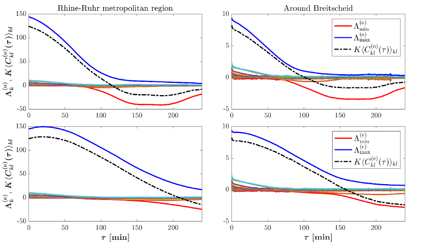
We work out and with empirical data of velocities during the time period from 15:00 to 20:00, i.e., min, for each workday. The largest time lag is restricted to 240 min. We further average and over 64 discontinuous workdays to remove the effect of noise and then symmetrize them for spectral decomposition. In figure 3, we show the eigenvalues of , x=e or o, versus the time lag for empirical data of the Rhine-Ruhr metropolitan region as well as around the motorway intersection near Breitscheid. The largest and the smallest eigenvalues are separated from other eigenvalues that are close to zero. In contrast to the case of a correlation matrix without time lags, the smallest eigenvalue becomes negative and gradually prevails over the largest eigenvalue as the time lag becomes larger. Put differently, with increasing, the dominant eigenvalue shifts from the largest eigenvalue to the smallest eigenvalue. We define the spectral transition as a change of dominant eigenvalues from positive values to negative values. The transition point corresponds to the time lag at which the sign changes. Such spectral transition happens for both motorway networks. The previous study [16] on the correlations in traffic without time lags reveals that the dominant eigenvalue, i.e. the largest positive eigenvalue, indicates the collective behavior of motorway sections. Here the transition of the dominant eigenvalue from positive values to negative values might hint a potential transition in traffic behavior.
For a correlation matrix without time lags in financial markets, the largest eigenvalue is in proportion to the average of all elements in the correlation matrix [35, 36, 37, 38]. For correlation matrices with time lags in traffic, the average correlations and are not exactly proportional to the largest eigenvalues of and , but shift from being nearly proportional to the largest eigenvalues to being nearly proportional to the smallest eigenvalues, as also shown in figure 3. Once more, a transition from positive values to negative values shows up in the evolution of either or . The transition occurs when the average correlation vanishes, i.e., or . It is worth mentioning that the transition in the original cases is earlier than in the extended ones, see figure 3. This difference may be traced back to the definition of extended correlations: the lagged time series includes ever more data outside the length of time series with increasing, effectively lowering the extended correlations than the original correlations at large .
3 Indicator correlations and congestion duration
The empirical results manifest a transition in the time evolution of eigenvalues. Is this transition related to traffic congestion? If yes, what kind of relation? One of the quantities to be measured is the congestion duration, a time period during which the velocity is below a threshold, e.g. 60 km/h. Thus, we can answer the questions just posed by replacing the time series of velocities with those of indicators for free or congested traffic, i.e. of traffic phases. This facilitates the construction of a simple model that we numerically analyze in five scenarios with different congestion durations and different shapes of congestion propagation in section 3.1. We observe transition points in the evolution of eigenvalues and explore their relation to congestion duration in section 3.2.
3.1 Spectral transitions related to congestion durations
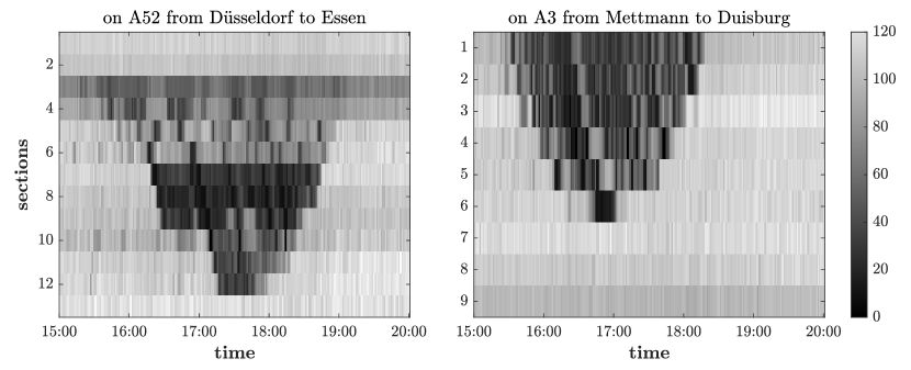
Figure 4 displays two empirical data matrices of velocities during afternoon rush hours on Jan. 18, 2017. The data matrices visualize the backward propagation of congestion, where the dark grey areas stand for low velocities, implying congested traffic phase, while the light grey areas for high velocities, implying free traffic phase. Both shapes of congestion propagation are similar to a triangle or a trapezium. To analyze the influences of congestion duration on the transition in the evolution of eigenvalues, we conduct five scenarios. We define an indicator of traffic phases on section at time as
| (19) |
which entries into a data matrix , simulated as follows. The time series in the data matrix are sorted in a descending oder of congestion duration of sections so that the time series with the longest congestion duration is the top row of , while the time series with the shortest duration () is the bottom row of . The congestion starts first at the top section and propagates backward to the bottom section in with gradually reduced durations from to . We also assume the time of backward propagation from one section to its nearest neighbouring section is one minute and the congestion duration is symmetrically located in the center of a time series with length , thereby forming the shape of a inverted pyramid or trapezoid as . Given for the top time series and for the bottom time series, we can determine the number of sections by
| (20) |
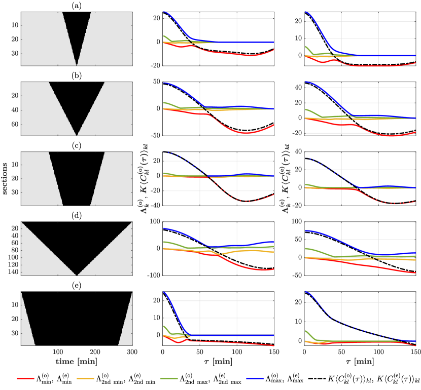
With a given and an obtained , we can set up a data matrix with binary values. Each row of the data matrix contains an indicator time series of a section, where zero is given in congestion duration and one is outside the congestion duration. Fixing the the length of time series min, we thus simulate five data matrices, as shown in figure 5, with different parameters and , listed in Table 1.
| \hlineB2 scenario | |||||||
|---|---|---|---|---|---|---|---|
| [min] | [min] | [min] | [min] | [min] | [min] | ||
| (a) | 38 | 2 | 37.5 | 39.5 | 2 | ||
| (b) | 75 | 2 | 56.5 | 62.5 | 6 | ||
| (c) | 39 | 59.5 | 69.5 | 10 | |||
| (d) | 149 | 2 | 64.5 | 91.5 | 27 | ||
| (e) | 38 | 30.5 | 130.5 | 100 | |||
| \hlineB2 |
With each of the five simulated data matrices, we work out the two kinds of correlation matrices , x=e or o, in terms of different time lags. For extended correlations, the extended part of time series are from free phases, i.e., , as the congestion found during afternoon rush hours has been resolved during the long night time. Diagonalizing each correlation matrix, we obtain the eigenvalues versus time lags visualized in figure 5. For the same longest congestion duration , e.g., for scenarios (b) and (c) and for scenarios (d) and (e), the different shortest durations lead to different congestion shapes and distinct differences . These have an influence on the remarkable transitions of the largest and the smallest eigenvalues, leading to a time gap between them. They also influence the point when the average correlation vanishes, i.e.,
| (21) |
When in scenarios (b) and (c), the remarkable transitions in the largest and the smallest eigenvalues are very close to the point at which the average correlation vanishes. Most interestingly, for scenario (c) which contains neither the smallest min (e.g., in scenarios (a), (b) and (d)) nor the largest (e.g., in scenarios (d) and (e)), the remarkable transitions in the largest and the smallest eigenvalues almost overlap with the vanishing of the average correlations at about 60 min. Increasing the duration to around in scenarios (d) and (e), the transitions in the largest and the smallest eigenvalues are more mild in extended correlations than in original correlations, leaving a wide gap between the two eigenvalues in extended correlations.
As those results show, we may utilize the vanishing of the average correlations as a substitute for the transition in the dominant eigenvalues. This substitution helps to quantify the difference between transition points and of dominant eigenvalues, which are obtained by minimizing the absolute value of the average correlation to make the average correlation as close to zero as possible,
| (22) |
as the average correlation typically does not become exactly zero. This difference is large when , but relatively small when , as listed in table 1. We further corroborate these observations by working out the transition points as function of the average congestion duration and the corresponding standard deviation. The average and the variance of congestion durations are given by
| (23) |
respectively. We use the standard deviation .
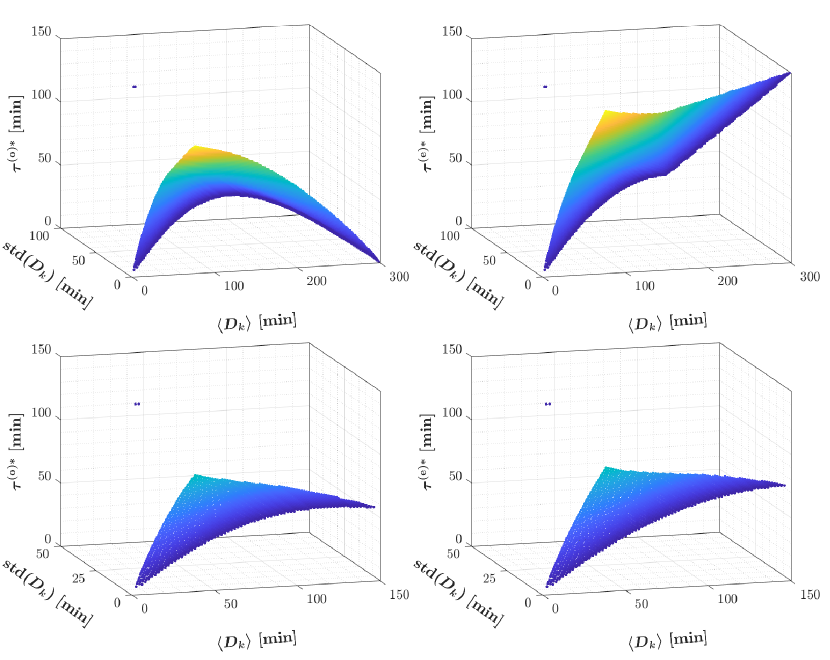
We let run from 2 to and from to with a duration step of 2 min. This generates different combinations of and . Each combination of and yields a data matrix, which results in an average congestion duration , a standard deviation of congestion durations , and a transition point with x=o or e. Figure 6 shows a nonlinear dependency of on and . For original and extended correlations, with min, the dependencies are very similar when but rather different when . In the latter case, the extended correlation might be distorted by appending the indicators of free traffic phases to the lagged indicator time series, or the vanishing of the extended correlations might not correctly reflect the transition point of the dominant eigenvalue. We find large standard deviations around . The longer the considered, the larger the differences and the standard deviations. For min, the original and the extended correlations show similar dependencies with relatively low standard deviations. Thus, we restrict our study to the scenarios with in the sequel.
3.2 Spectral transitions at the vanishing of correlations
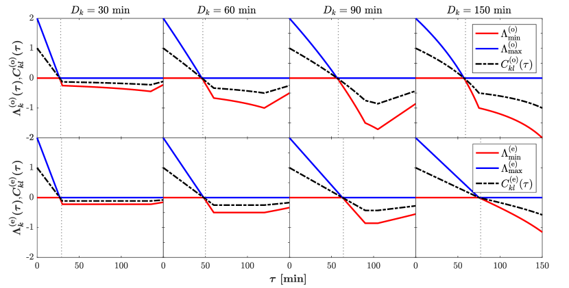
Each simulated data matrix shown in figure 5 contains time series of indicators, where . To simplify the situation, here we reduce the number of time series to two, i.e. , and simulate data matrices of indicators with min. We assume that the time series in the first row of the data matrix is from section and the time series in the second row is from section . The congestion for each time series is located symmetrically around the center of the time series of length with zero values. The other values in each time series are one, indicating free phases. For equal congestion duration, i.e., , the original and extended correlation can be considered as the autocorrelation of the same time series with lengths and , respectively. Therefore, the four elements at a certain time lag are the same, i.e., , where x=o or e. In this setting, the correlation averaged over four elements is equal to any element in the correlation matrix . Due to the symmetry of this correlation matrix, we have . The resulting two eigenvalues for each correlation matrix are shown in figure 7. For congestion duration , the transitions in the largest and the smallest eigenvalues intersect with the point when . The vanishing of the correlation between the two sections, therefore, signals the transition point of the dominant eigenvalue of a correlation matrix,
| (24) |
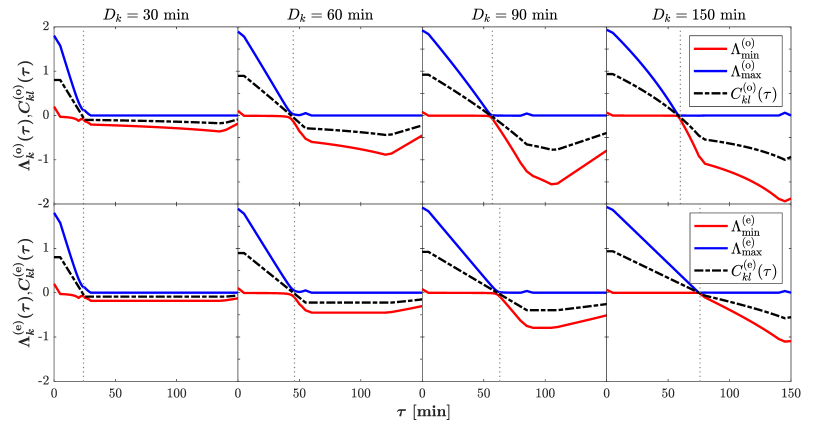
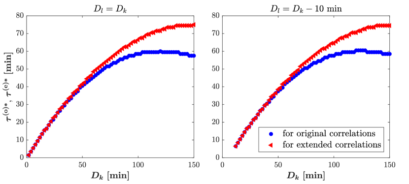
In reality, since the propagation and relief of congestion take time, the congestion durations for two sections are seldom the same, as shown in figure 4. Here we set the propagation time to be , such that . The congestion for each section also lies symmetrically around the center of the time series. In this scenario, the four elements in each correlation matrix are different. We symmetrize each correlation matrix before obtaining the eigenvalues from . Setting min, we find the transition point in eigenvalues overlaps quite well with the point when , despite the fact that is one of the off-diagonal elements in the correlation matrix instead of the average of four elements in this matrix. To enlarge the effect of propagation time on the transition points of eigenvalues, we consider min. As shown in figure 8, the transitions in the largest and the smallest eigenvalues are still very close to the point when . In contrast to the congestion duration with different values, , and 150 min, the effect of duration difference is negligible. This shows that as long as the difference between two durations is short enough, e.g. min, the transition points in dominant eigenvalues can be estimated by equation (24).
Using the vanishing of correlations, we find a relation between the transition point or in the dominant eigenvalues and the congestion duration when and min, displayed in figure 9. With increase of the congestion duration, the transition moves towards large values in a nonlinear fashion. For small congestion durations, the transition points for the original and extended correlations are close. For large congestion durations, a large deviation in the transition points emerges for the two kinds of correlations. The duration difference has little influence.
4 Analytical treatment of the model for correlation matrices
In our previous analyses, we explored the transition points of eigenvalues. We now consider a simplified, schematic version of the model that captures the features found. We normalize the indicators for original and extended correlations in section 4.1. We model five scenarios with equal and unequal durations of congestion in sections 4.2 and 4.3, respectively.
4.1 Normalized indicators for original and extended correlations
We define a relative congestion duration by normalizing to the length of time series
| (25) |
and accordingly relative time lags
| (26) |
For original correlations, the mean value and the standard deviation are calculated for the used time series of length , not for the whole time series of length . We express them in terms of and as
| (27) |
and
| (28) |
respectively. In an indicator time series , for free traffic phases and for congested traffic phases. Here and in the following calculations, we split the sum running from to or into three sums, running from 1 to , to , and to or , in which takes the values , and , respectively. For extended correlations, the time series of length is used. Thus, the mean value and the standard deviation, given by
| (29) |
and
| (30) |
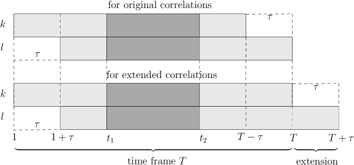
are different from the ones for the original correlations. As seen in figure 10, for each kind of correlation, given a non-zero time lag, the time series of section lags behind the time series of section , but these two time series have the same mean values and standard deviations. We then normalize the indicators of free and congested phases for original and extended correlations to zero mean and unit standard deviation,
| (31) | |||||
| (32) | |||||
| (33) | |||||
| (34) |
We notice that for original as well as for extended correlations, the normalized indicator of free traffic phases is the negative of the reciprocal of the normalized indicator of congested traffic phases, leading to and . Furthermore, reducing to zero results in and yields and .
Scenario 1
Scenario 2

4.2 Scenarios with equal durations of congestion
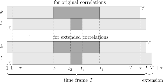
If the times at which the congestions on two sections and start and end coincide, e.g. both start at 16:00 and end at 17:00 on a workday, the two time series of indicators have equal congestion duration . We refer to the scenario that the duration is larger than the positive time lag , i.e. , as scenario 1 and to the scenario that the duration is smaller than or equal to , i.e. , as scenario 2, as sketched in figure 10. For both scenarios, the time lag is always smaller than the start time of the congestion and the congestion is always symmetrically located in a time series with length , i.e., and . Here, also requires . Otherwise, will be zero.
According to the definitions of original correlations (10) and extended correlations (15), we expand the sum of products of two normalized indicators into several parts, which are for free phases with free phases, congested phases with congested phases, free phases with congested phases and congested phases with free phases during different correlated times. In this way, we obtain expressions of correlations in terms of and . For scenario 1, the two kinds of correlations read
| (35) | |||||
and
| (36) | |||||
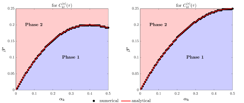
respectively. As seen in figure 7, when the correlations vanish and , the spectrum transition occurs. We therefore associate the relative time lag of transition point with the relative congestion duration , i.e.,
| (37) |
for original correlations and
| (38) |
for extended correlations. Figure 11 displays the dependence of relative time lag on relative congestion duration simulated by equations (37) and (38), Here we restrict the congestion duration to half the length of the time series, i.e., , as analyzed at the end of section 3.1. For both kinds of correlations, the analytical results perfectly match with the numerical ones. The dependent curve is a transition curve that is connected by all transition points and separates the system into two spectral phases. Below the curve, it is the first spectral phase that the largest eigenvalue dominates in the system. Above the curve, it transforms to the second spectral phase that the smallest eigenvalue dominates. According to equations (37) and (38), the maximal at for original correlations and the maximal at for extended correlations, which means the maximal transition points are at min and at min for original and extended correlation, respectively. The two values are close to the simulated transition points min and min for scenario (c) with min and min listed in table 1. The slight differences in transition points are account of different constraints, as the simulation in scenario (c) is for 39 sections with gradually changed congestion durations, while the model in scenario 1 only for two sections with the same congestion duration. Despite of this, we notice that the congestion duration plays a critical role in the transition of eigenvalues.
For scenario 2, despite the fact that the correlations in terms of and can be derived, we cannot use the vanishing of correlations to find a relation between and under the constraints and .
4.3 Scenarios with differing durations of congestion
Scenario 3
Scenario 4
Scenario 5
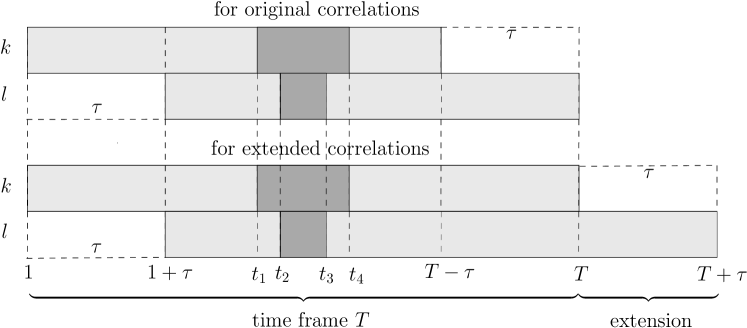
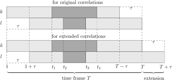
If the congestion on section starts first and propagates to section , the congestion on section will start a little later but will end earlier than on section , leading to , where and , as shown in figure 12. For instance, the congestion duration for section is from 15:50 to 17:10 and for section from 16:00 to 17:00. Here we assume the congestion is symmetrically located in each time series of length , such that , and . In the following, we consider three scenarios, namely scenarios 3, 4 and 5, where in scenarios 3 and 4, the time lag is smaller than or equal to the short congestion duration , but in scenario 5, the time lag larger than or equal to the long congestion duration . Moreover, in scenarios 3 and 5, the time lag is larger than or equal to the half difference of congestion duration , but in scenario 4, it is smaller than half the difference of congestion duration . To distinguish the five scenarios clearly, we list the constraints for each of them in table 2. In terms of the relative congestion durations and for sections and as well as the relative time lag , we work out the correlation coefficient,
| (39) | |||||
| scenario | constraint 1 | constraint 2 | constraint 3 |
|---|---|---|---|
| Scenario 1 | |||
| Scenario 2 | |||
| Scenario 3 | |||
| Scenario 4 | |||
| Scenario 5 | |||
for original correlations, and
| (40) | |||||
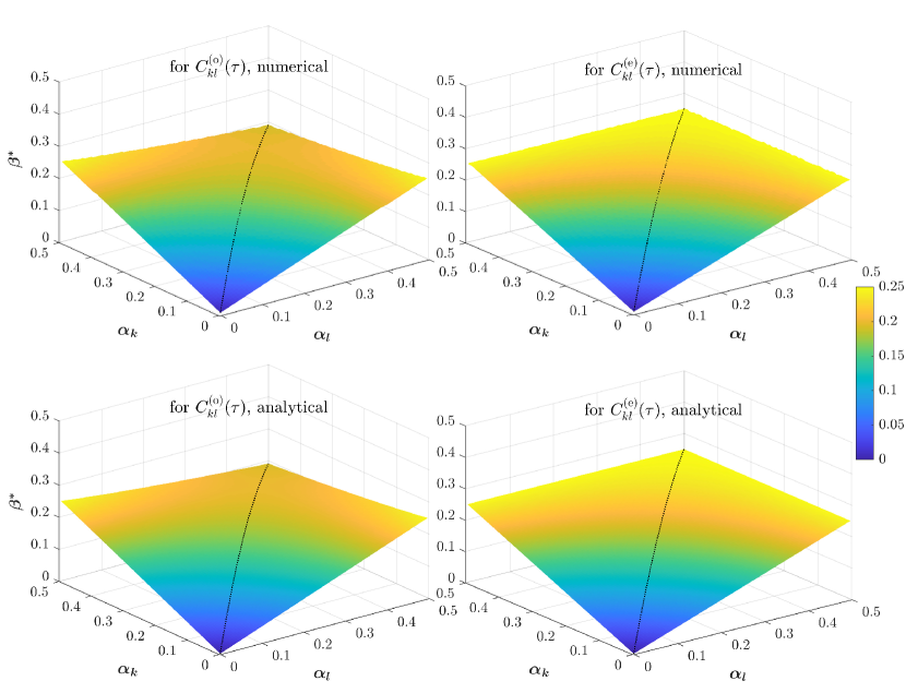
for extended ones. To find the transition point, we use the vanishing of the original correlations, i.e. , and thereby obtain
| (41) |
Analogously, we arrive at
| (42) |
by solving for extended correlations.
In the range , and , the dependence of on and manifests itself as a surface shown in a three-dimensional plot in figure 13. The analytical results are very close to the numerical ones. The colors of the surface correspond to values of regardless of how and combine. Equations (41) and (42) with result in equations (37) and (38). The black dotted line on surfaces in figure 13 corresponds to scenario 1 with equal congestion duration. Each surface in figure 13 separates spectral phase 1 from spectral phase 2. The former, under the surface, is governed by the largest, positive eigenvalue while the latter, above the surface, is dominated by the smallest, negative eigenvalue. Obviously, when the congestion durations for either or both sections are around , there are many high values of colored red on the surface, implying large transition points, before which the largest eigenvalue prevails over the smallest one for a long time. In contrast, when the congestion durations on both sections approach 0, some low values of colored blue on the surface are visible, suggesting small transition points, which further reveals the smallest eigenvalues are quickly victorious over the largest one. In other words, the largest eigenvalue dominates longer if the congestion duration of either section is around but shorter if the congestion durations of both sections approach 0. From another point of view, when given any two of the three quantities , and , we are able to infer the remaining quantity from the three-dimensional surface, especially the congestion duration or . Notably, when , equations (41) and (42) are simplified to equations (37) and (38), respectively.
For scenarios 4 and 5, a relation that fulfills the constraints , and at the same time is absent among , and .
5 Conclusions
The congestion propagation to neighbouring motorway sections gives rise to the correlated traffic behavior. The full time-lagged correlation matrix of a motorway network encodes the congestion characteristics among other information. We showed how to reveal them by the interesting spectra.
A correlation matrix without time lags is symmetric and semi-positive definite, resulting in real and positive eigenvalues. With a time lag, however, this correlation matrix becomes asymmetric and the resulting eigenvalues are complex. To obtain real eigenvalues, one can addresses the time-lagged correlation matrix either by singular value decomposition or by eigenvalue decomposition after the symmetrization of the correlation matrix. Here, we took up the latter approach for the time-lagged correlation matrix of velocities. In empirical studies, we found a transition of the dominant eigenvalue from a positive value to a negative one as function of the time lag. This transition is related to the average of all elements in the correlation matrix. We set up a model by using indicator time series of traffic phases. Our numerical simulation show that this transition occurs when the average correlation (or the cross-correlation) vanishes for the dimension of the correlation matrix larger than (or equal to) two. Moreover, our numerical simulations of scenarios with different congestion durations reveal a nonlinear dependence of the transition point on the congestion duration. The nonlinear dependence for the latter with time-lagged correlation can be analytically described by a simple, schematic indicator model that we set up. With this analytical model, the congestion duration can be readily extracted from spectral transition of the correlation matrices.
In carrying out these studies, we also studied a generic statistics issue occurring when looking at time-lagged correlations. When the time lag is very large comparing to the fixed length of time series, the statistics become rather poor. We put forward an extended time-lagged correlation, relative to the original, widely used one. In the extended time-lagged correlation we used the time series of the full length as the leading time series, and the one including additional data points at the end as the lagged time series, such that leading and lagged time series always have the same length. By comparing the two kinds of time-lagged correlations, we found the extended correlation is smaller than the original one at a given time lag. Furthermore, we found when the congestion duration is larger than the half time series, a large divergence emerges in the nonlinear dependence of the spectral transition point on the congestion duration. This phenomenon implies a limitation of congestion duration to half of the time series in the analysis of its relation with spectral transition.
Acknowledgments
We gratefully acknowledge the support from Deutsche Forschungsgemeinschaft (DFG ) within the project “Korrelationen und deren Dynamik in Autobahnnetzen” (No. 418382724). We thank Strassen.NRW for providing the empirical traffic data.
References
- [1] Cambridge Systematics. Traffic congestion and reliability: Trends and advanced strategies for congestion mitigation. Technical report, United States. Federal Highway Administration, 2005.
- [2] Inrix. Inrix 2022 global traffic scorecard. https://inrix.com/scorecard/, 01 2023.
- [3] Michael C Münnix, Takashi Shimada, Rudi Schäfer, Francois Leyvraz, Thomas H Seligman, Thomas Guhr, and H Eugene Stanley. Identifying states of a financial market. Sci. Rep., 2(1):1–6, 2012.
- [4] Qawi K Telesford, Sean L Simpson, Jonathan H Burdette, Satoru Hayasaka, and Paul J Laurienti. The brain as a complex system: using network science as a tool for understanding the brain. Brain Connect., 1(4):295–308, 2011.
- [5] Arturo Roman Messina. Inter-area oscillations in power systems: a nonlinear and nonstationary perspective. Springer Science & Business Media, 2009.
- [6] Linyin Cheng, Amir AghaKouchak, Eric Gilleland, and Richard W Katz. Non-stationary extreme value analysis in a changing climate. Clim. Change, 127:353–369, 2014.
- [7] Boris Podobnik, Duan Wang, Davor Horvatic, Ivo Grosse, and H Eugene Stanley. Time-lag cross-correlations in collective phenomena. EPL, 90(6):68001, 2010.
- [8] Mohammadreza Saeedmanesh and Nikolas Geroliminis. Dynamic clustering and propagation of congestion in heterogeneously congested urban traffic networks. Transp. Res. Proc., 23:962–979, 2017.
- [9] Leonardo Bellocchi and Nikolas Geroliminis. Unraveling reaction-diffusion-like dynamics in urban congestion propagation: Insights from a large-scale road network. Sci. Rep., 10(1):1–11, 2020.
- [10] Meead Saberi, Homayoun Hamedmoghadam, Mudabber Ashfaq, Seyed Amir Hosseini, Ziyuan Gu, Sajjad Shafiei, Divya J Nair, Vinayak Dixit, Lauren Gardner, S Travis Waller, et al. A simple contagion process describes spreading of traffic jams in urban networks. Nat. Commun., 11(1):1616, 2020.
- [11] Shanshan Wang, Sebastian Gartzke, Michael Schreckenberg, and Thomas Guhr. Quasi-stationary states in temporal correlations for traffic systems: Cologne orbital motorway as an example. J. Stat. Mech. Theory Exp., 2020(10):103404, 2020.
- [12] Sebastian M Krause, Lars Habel, Thomas Guhr, and Michael Schreckenberg. The importance of antipersistence for traffic jams. EPL, 118(3):38005, 2017.
- [13] Shanshan Wang, Sebastian Gartzke, Michael Schreckenberg, and Thomas Guhr. Transitions between quasi-stationary states in traffic systems: Cologne orbital motorway as an example. J. Stat. Mech. Theory Exp., 2023:093401, 2023.
- [14] Boris S Kerner. Understanding Real Traffic. Springer, 2021.
- [15] Sebastian Gartzke, Shanshan Wang, Thomas Guhr, and Michael Schreckenberg. Spatial correlation analysis of traffic flow on parallel motorways in germany. Physica A, 599:127367, 2022.
- [16] Shanshan Wang, Sebastian Gartzke, Michael Schreckenberg, and Thomas Guhr. Collective behavior in the North Rhine-Westphalia motorway network. J. Stat. Mech. Theory Exp., 2021:123401, 2021.
- [17] Shanshan Wang, Michael Schreckenberg, and Thomas Guhr. Identifying subdominant collective effects in a large motorway network. J. Stat. Mech. Theory Exp., 2022:113402, 2022.
- [18] Shanshan Wang, Michael Schreckenberg, and Thomas Guhr. Response functions as a new concept to study local dynamics in traffic networks. Physica A, 626:129116, 2023.
- [19] Sebastian Gartzke, Shanshan Wang, Thomas Guhr, and Michael Schreckenberg. Response of fundamental traffic observables: Differentiate patterns and determine propagation velocity of congested traffic. In preparation, 2023.
- [20] Jianjiang Yang, Lee D Han, Phillip B Freeze, Shih-Miao Chin, and Ho-Ling Hwang. Short-term freeway speed profiling based on longitudinal spatiotemporal dynamics. Transp. Res. Rec., 2467(1):62–72, 2014.
- [21] Corrado De Fabritiis, Roberto Ragona, and Gaetano Valenti. Traffic estimation and prediction based on real time floating car data. In 2008 11th international IEEE conference on intelligent transportation systems, pages 197–203. IEEE, 2008.
- [22] Lutz Neubert, Ludger Santen, Andreas Schadschneider, and Michael Schreckenberg. Single-vehicle data of highway traffic: A statistical analysis. Phys. Rev. E, 60(6):6480, 1999.
- [23] TL Pan, Agachai Sumalee, Ren-Xin Zhong, and Nakorn Indra-Payoong. Short-term traffic state prediction based on temporal–spatial correlation. IEEE Trans. Intell. Transp. Syst., 14(3):1242–1254, 2013.
- [24] Feng Guo, Xin Gu, Zhaoxia Guo, Yucheng Dong, and Stein W Wallace. Understanding the marginal distributions and correlations of link travel speeds in road networks. Sci. Rep., 10(1):11821, 2020.
- [25] Zuduo Zheng, Soyoung Ahn, and Christopher M Monsere. Impact of traffic oscillations on freeway crash occurrences. Accid. Anal. Prev., 42(2):626–636, 2010.
- [26] Srinivasa Ravi Chandra and Haitham Al-Deek. Cross-correlation analysis and multivariate prediction of spatial time series of freeway traffic speeds. Transp. Res. Rec., 2061(1):64–76, 2008.
- [27] Lu Sun. Spectral and time-frequency analyses of freeway traffic flow. J. Adv. Transp., 48(7):821–857, 2014.
- [28] Tenny Lam and Richard Rothery. The spectral analysis of speed fluctuations on a freeway. Transp. Sci., 4(3):293–310, 1970.
- [29] Wolfgang Knospe, Ludger Santen, Andreas Schadschneider, and Michael Schreckenberg. Single-vehicle data of highway traffic: Microscopic description of traffic phases. Phys. Rev. E, 65(5):056133, 2002.
- [30] Wolfgang Knospe, Ludger Santen, Andreas Schadschneider, and Michael Schreckenberg. A realistic two-lane traffic model for highway traffic. Phys. A Math. Gen., 35(15):3369, 2002.
- [31] Boris S Kerner. The Physics of Traffic: Empirical Freeway Pattern Features, Engineering Applications, and Theory. Springer, 2012.
- [32] OpenStreetMap. Copyright and License. https://www.openstreetmap.org/copyright, 2021.
- [33] Open Knowledge Foundation. Open Data Commons Open Database License (ODbL) v1.0. https://opendatacommons.org/licenses/odbl/1-0/, 2021.
- [34] QGIS. Documentation for QGIS 3.4. https://docs.qgis.org/3.4/en/docs/, 2020.
- [35] Yuriy Stepanov, Philip Rinn, Thomas Guhr, Joachim Peinke, and Rudi Schäfer. Stability and hierarchy of quasi-stationary states: financial markets as an example. J. Stat. Mech: Theory Exp., 2015(8):P08011, 2015.
- [36] Vasiliki Plerou, Parameswaran Gopikrishnan, Bernd Rosenow, Luis A Nunes Amaral, Thomas Guhr, and H Eugene Stanley. Random matrix approach to cross correlations in financial data. Phys. Rev. E, 65(6):066126, 2002.
- [37] Dong-Ming Song, Michele Tumminello, Wei-Xing Zhou, and Rosario N Mantegna. Evolution of worldwide stock markets, correlation structure, and correlation-based graphs. Phys. Rev. E, 84(2):026108, 2011.
- [38] Hirdesh K Pharasi, Kiran Sharma, Anirban Chakraborti, and Thomas H Seligman. Complex market dynamics in the light of random matrix theory. In New Perspectives and Challenges in Econophysics and Sociophysics, pages 13–34. Springer, 2019.