[1]\fnmBennet \surGebken

[1]\orgdivInsitute of Mathematics, \orgnamePaderborn University, \orgaddress\streetWarburger Str. 100, \cityPaderborn, \postcode33098, \countryGermany

A note on the convergence of deterministic gradient sampling in nonsmooth optimization

Abstract

Approximation of subdifferentials is one of the main tasks when computing descent directions for nonsmooth optimization problems. In this article, we propose a bisection method for weakly lower semismooth functions which is able to compute new subgradients that improve a given approximation in case a direction with insufficient descent was computed. Combined with a recently proposed deterministic gradient sampling approach, this yields a deterministic and provably convergent way to approximate subdifferentials for computing descent directions.

keywords:
Nonsmooth optimization, Nonsmooth analysis, Nonconvex optimization, Gradient sampling

1 Introduction

Nonsmooth optimization is concerned with the optimization of a function f:ℝn→ℝ:𝑓→superscriptℝ𝑛ℝf:\mathbb{R}^{n}\rightarrow\mathbb{R} which is not necessarily continuously differentiable. For such functions, one cannot rely on the gradient for describing the local behavior around a given point. As a replacement, generalized concepts from nonsmooth analysis can be employed. If the objective is still locally Lipschitz continuous, as is the case in many practical applications, then the standard approach is to use the Clarke subdifferential βˆ‚f𝑓\partial f [1]. However, since βˆ‚f​(x)𝑓π‘₯\partial f(x) reduces to the gradient if f𝑓f is continuously differentiable at xπ‘₯x, and since f𝑓f is typically continuously differentiable almost everywhere, the Clarke subdifferential cannot be used to capture nonsmoothness numerically. To circumvent this issue, the (Goldstein) Ξ΅πœ€\varepsilon-subdifferential βˆ‚Ξ΅fsubscriptπœ€π‘“\partial_{\varepsilon}f [2] may be used instead, which is the convex hull of all Clarke subdifferentials in an Ξ΅πœ€\varepsilon-ball around a given point. For the Ξ΅πœ€\varepsilon-subdifferential, it is sufficient for xπ‘₯x to have a distance of at most Ξ΅πœ€\varepsilon to a nonsmooth point of f𝑓f to capture the nonsmoothness. As such, it can be interpreted as a stabilized version of the Clarke subdifferential.

It is well-known that the element vΒ―βˆˆβˆ’βˆ‚Ξ΅f​(x0)¯𝑣subscriptπœ€π‘“subscriptπ‘₯0\bar{v}\in-\partial_{\varepsilon}f(x_{0}) with the smallest norm is a descent direction for f𝑓f at x0subscriptπ‘₯0x_{0} [2, 1]. Unfortunately, the full Ξ΅πœ€\varepsilon-subdifferential that is required to compute this direction is rarely available in practice and has to be approximated instead. To this end, in the gradient sampling method [3, 4, 5], the idea is to approximate βˆ‚Ξ΅f​(x0)subscriptπœ€π‘“subscriptπ‘₯0\partial_{\varepsilon}f(x_{0}) by the convex hull of the gradients at randomly generated points in the Ξ΅πœ€\varepsilon-ball around x0subscriptπ‘₯0x_{0} where f𝑓f is differentiable. While this is easy to implement and convergence can be shown with probability 111, randomly computing gradients means that one generally computes more gradients than would be necessary. Furthermore, a good approximation may require a large and a priori unknown number of sample points (which is highlighted in Appendix A). As an alternative, in [6, 7, 8], a deterministic sampling approach was used. There, the idea is to compute the approximation of βˆ‚Ξ΅f​(x0)subscriptπœ€π‘“subscriptπ‘₯0\partial_{\varepsilon}f(x_{0}) iteratively, by starting with W={ΞΎ}π‘Šπœ‰W=\{\xi\} for a subgradient ΞΎβˆˆβˆ‚f​(x0)πœ‰π‘“subscriptπ‘₯0\xi\in\partial f(x_{0}) at x0subscriptπ‘₯0x_{0}, and then adding new elements of βˆ‚Ξ΅f​(x0)subscriptπœ€π‘“subscriptπ‘₯0\partial_{\varepsilon}f(x_{0}) to Wπ‘ŠW until conv(W)convπ‘Š\operatorname*{conv}(W) is a satisfactory approximation. The mechanism for finding new elements of βˆ‚Ξ΅f​(x0)subscriptπœ€π‘“subscriptπ‘₯0\partial_{\varepsilon}f(x_{0}) is based on the observation that if v𝑣v is a direction that yields less descent than expected (based on the current approximation conv(W)convπ‘Š\operatorname*{conv}(W)), then there has to be a point x0+t​vsubscriptπ‘₯0𝑑𝑣x_{0}+tv with t>0𝑑0t>0 in the Ξ΅πœ€\varepsilon-ball at which a new subgradient ΞΎβ€²βˆˆβˆ‚f​(x0+t​v)βŠ†βˆ‚Ξ΅f​(x0)superscriptπœ‰β€²π‘“subscriptπ‘₯0𝑑𝑣subscriptπœ€π‘“subscriptπ‘₯0\xi^{\prime}\in\partial f(x_{0}+tv)\subseteq\partial_{\varepsilon}f(x_{0}) with ΞΎβ€²βˆ‰conv(W)superscriptπœ‰β€²convπ‘Š\xi^{\prime}\notin\operatorname*{conv}(W) can be sampled. To find such a t𝑑t, a subroutine based on bisection of the interval (0,Ξ΅/β€–vβ€–)0πœ€norm𝑣(0,\varepsilon/\|v\|) is used. While in [6, 7, 8], it was analyzed why this subroutine likely works (i.e., terminates) in practice and while termination was also observed in all numerical examples, a full proof (under reasonable assumptions for f𝑓f) was not given.

The goal of this note is to close the above mentioned gap in the convergence theory of the deterministic gradient sampling approach. The bisection algorithm in [6, 7, 8] is based on reformulating the problem of finding a new element of βˆ‚Ξ΅f​(x0)subscriptπœ€π‘“subscriptπ‘₯0\partial_{\varepsilon}f(x_{0}) as finding a point t>0𝑑0t>0 in which a certain nonsmooth function h:ℝ→ℝ:β„Žβ†’β„β„h:\mathbb{R}\rightarrow\mathbb{R} is increasing. The convergence issues arise in cases where the bisection converges to a critical point t¯¯𝑑\bar{t} of hβ„Žh (i.e., to a point t¯¯𝑑\bar{t} with 0βˆˆβˆ‚h​(tΒ―)0β„ŽΒ―π‘‘0\in\partial h(\bar{t})). To fix these issues, we replace hβ„Žh by a slightly modified function hc~subscriptβ„Ž~𝑐h_{\tilde{c}}. We then show convergence of the resulting method for the case where f𝑓f is weakly lower semismooth [9, 10] (meaning that βˆ’f𝑓-f is weakly upper semismooth). Since semismooth functions [11] are weakly lower semismooth, this case includes continuously differentiable functions, convex functions and piecewise differentiable functions [12]. As our result is essentially just concerned with the deterministic computation of new Ξ΅πœ€\varepsilon-subgradients (not necessarily in the context of [6, 7, 8]), it has also use in other methods based on gradient sampling, like [13, 14]. Our method has strong similarities to Procedure 4.1 in [15], which is used for the computation of new subgradients in a bundle framework. It is based on the same idea, but differs in the condition used for bisection and the stopping criterion.

The remainder of this article is structured as follows: In Section 2 we introduce the basics of gradient sampling and the bisection algorithm from [7] (which is identical to the one in [8] and almost identical to the one in [6]). In [7], the bisection was only a small part of a larger algorithm, but we will introduce it here in a stand-alone way for convenience. In Section 3 we construct the improved bisection algorithm and show its convergence when f𝑓f is weakly lower semismooth. In Section 4 we visualize the behavior of the improved bisection method in a simple example. Finally, in Section 5, we summarize our results and discuss possible directions for future research.

2 Computing descent directions for nonsmooth functions

In this section, we summarize the basic ideas of gradient sampling from [3, 4, 5, 6, 7, 8]. To this end, let f:ℝn→ℝ:𝑓→superscriptℝ𝑛ℝf:\mathbb{R}^{n}\rightarrow\mathbb{R} be locally Lipschitz continuous. The Clarke subdifferential [1] of f𝑓f at xβˆˆβ„nπ‘₯superscriptℝ𝑛x\in\mathbb{R}^{n} is given by

βˆ‚f​(x):=convassign𝑓π‘₯conv\displaystyle\partial f(x):=\operatorname*{conv} ({ΞΎβˆˆβ„n:βˆƒ(xj)jβˆˆβ„nβˆ–Ξ©Β withΒ limjβ†’βˆžxj=xΒ andΒ \displaystyle\left(\left\{\xi\in\mathbb{R}^{n}:\exists(x^{j})_{j}\in\mathbb{R}^{n}\setminus\Omega\text{ with }\lim_{j\rightarrow\infty}x^{j}=x\text{ and }\right.\right. (1)
limjβ†’βˆžβˆ‡f(xj)=ΞΎ}),\displaystyle\left.\left.\lim_{j\rightarrow\infty}\nabla f(x^{j})=\xi\right\}\right),

where Ξ©βŠ†β„nΞ©superscriptℝ𝑛\Omega\subseteq\mathbb{R}^{n} is the set of points at which f𝑓f is not differentiable. (By Rademacher’s Theorem [1], ΩΩ\Omega has measure zero.) The elements of βˆ‚f​(x)𝑓π‘₯\partial f(x) are called (Clarke) subgradients. In theory, the Clarke subdifferential can be used similarly to the standard gradient, as it can be used in generalized versions of results like the mean value theorem, the chain rule and optimality conditions [1]. In practice however, there are severe problems: βˆ‚f​(x)𝑓π‘₯\partial f(x) only captures the nonsmoothness of f𝑓f if xπ‘₯x is a point where f𝑓f is not continuously differentiable, which is typically a null set. Furthermore, when x∈Ωπ‘₯Ξ©x\in\Omega, there is no general way of computing the full subdifferential, i.e., all subgradients. Instead, a reasonable assumption is that we can only evaluate a single, arbitrary subgradient from βˆ‚f​(x)𝑓π‘₯\partial f(x) at any xβˆˆβ„nπ‘₯superscriptℝ𝑛x\in\mathbb{R}^{n}. Further explanations and examples for these issues can be found in [16]. To circumvent these problems, a more suitable object to use as a generalized derivative for constructing descent methods is the (Goldstein) Ξ΅πœ€\varepsilon-subdifferential [2]

βˆ‚Ξ΅f​(x):=conv(⋃y∈BΡ​(x)βˆ‚f​(y)),assignsubscriptπœ€π‘“π‘₯convsubscript𝑦subscriptπ΅πœ€π‘₯𝑓𝑦\displaystyle\partial_{\varepsilon}f(x):=\operatorname*{conv}\left(\bigcup_{y\in B_{\varepsilon}(x)}\partial f(y)\right),

where Ξ΅β‰₯0πœ€0\varepsilon\geq 0, BΡ​(x):={yβˆˆβ„n:β€–yβˆ’x‖≀Ρ}assignsubscriptπ΅πœ€π‘₯conditional-set𝑦superscriptℝ𝑛norm𝑦π‘₯πœ€B_{\varepsilon}(x):=\{y\in\mathbb{R}^{n}:\|y-x\|\leq\varepsilon\} and βˆ₯β‹…βˆ₯\|\cdot\| is the Euclidean norm. The elements of βˆ‚Ξ΅f​(x)subscriptπœ€π‘“π‘₯\partial_{\varepsilon}f(x) are called Ξ΅πœ€\varepsilon-subgradients. The Ξ΅πœ€\varepsilon-subdifferential can be interpreted as a β€œstabilized” Clarke subdifferential. In particular, it can be used to compute descent directions, as we demonstrate in the following.

Let x0βˆˆβ„nsubscriptπ‘₯0superscriptℝ𝑛x_{0}\in\mathbb{R}^{n}, vβˆˆβ„nβˆ–{0}𝑣superscriptℝ𝑛0v\in\mathbb{R}^{n}\setminus\{0\} and Ξ΅>0πœ€0\varepsilon>0. Then a simple application of the mean value theorem ([1], Theorem 2.3.7) shows that

f​(x0+t​v)≀f​(x0)+t​maxΞΎβˆˆβˆ‚Ξ΅f​(x0)⁑⟨ξ,vβŸ©βˆ€t∈(0,Ξ΅β€–vβ€–].formulae-sequence𝑓subscriptπ‘₯0𝑑𝑣𝑓subscriptπ‘₯0𝑑subscriptπœ‰subscriptπœ€π‘“subscriptπ‘₯0πœ‰π‘£for-all𝑑0πœ€norm𝑣\displaystyle f\left(x_{0}+tv\right)\leq f(x_{0})+t\max_{\xi\in\partial_{\varepsilon}f(x_{0})}\langle\xi,v\rangle\quad\forall t\in\left(0,\frac{\varepsilon}{\|v\|}\right]. (2)

Thus, directions v𝑣v with ⟨ξ,v⟩<0πœ‰π‘£0\langle\xi,v\rangle<0 for all ΞΎβˆˆβˆ‚Ξ΅f​(x0)πœ‰subscriptπœ€π‘“subscriptπ‘₯0\xi\in\partial_{\varepsilon}f(x_{0}) are descent directions for f𝑓f at x0subscriptπ‘₯0x_{0}. Based on convex analysis [17], the direction that minimizes the maximum of the inner products on the right-hand side of (2), called the Ξ΅πœ€\varepsilon-steepest descent direction, can be computed as

vΒ―:=βˆ’arg​minΞΎβˆˆβˆ‚Ξ΅f​(x0)⁑‖ξ‖2.assign¯𝑣subscriptargminπœ‰subscriptπœ€π‘“subscriptπ‘₯0superscriptnormπœ‰2\displaystyle\bar{v}:=-\operatorname*{arg\,min}_{\xi\in\partial_{\varepsilon}f(x_{0})}\|\xi\|^{2}. (3)

It holds either vΒ―=0¯𝑣0\bar{v}=0, in which case 0βˆˆβˆ‚Ξ΅f​(x0)0subscriptπœ€π‘“subscriptπ‘₯00\in\partial_{\varepsilon}f(x_{0}) and x0subscriptπ‘₯0x_{0} is called Ξ΅πœ€\varepsilon-critical, or

⟨ξ,vΒ―βŸ©β‰€βˆ’β€–vΒ―β€–2<0βˆ€ΞΎβˆˆβˆ‚Ξ΅f​(x0)formulae-sequenceπœ‰Β―π‘£superscriptnorm¯𝑣20for-allπœ‰subscriptπœ€π‘“subscriptπ‘₯0\displaystyle\langle\xi,\bar{v}\rangle\leq-\|\bar{v}\|^{2}<0\quad\forall\xi\in\partial_{\varepsilon}f(x_{0}) (4)

and, due to (2),

f​(x0+Ξ΅β€–v¯‖​vΒ―)≀f​(x0)βˆ’Ξ΅β€‹β€–vΒ―β€–.𝑓subscriptπ‘₯0πœ€norm¯𝑣¯𝑣𝑓subscriptπ‘₯0πœ€norm¯𝑣\displaystyle f\left(x_{0}+\frac{\varepsilon}{\|\bar{v}\|}\bar{v}\right)\leq f(x_{0})-\varepsilon\|\bar{v}\|. (5)

Unfortunately, the full Ξ΅πœ€\varepsilon-subdifferential required to solve Problem (3) is rarely available in practice. Thus, the direction v¯¯𝑣\bar{v} has to be approximated.

2.1 Random gradient sampling

In the standard gradient sampling framework [3, 4, 5], the Ξ΅πœ€\varepsilon-subdifferential is approximated by randomly (independently and uniformly) sampling mβ‰₯n+1π‘šπ‘›1m\geq n+1 elements x1,…,xm∈BΡ​(x0)βˆ–Ξ©superscriptπ‘₯1…superscriptπ‘₯π‘šsubscriptπ΅πœ€subscriptπ‘₯0Ξ©x^{1},\dots,x^{m}\in B_{\varepsilon}(x_{0})\setminus\Omega and setting

W:={βˆ‡f​(x0),βˆ‡f​(x1),…,βˆ‡f​(xm)}βŠ†βˆ‚Ξ΅f​(x0).assignπ‘Šβˆ‡π‘“subscriptπ‘₯0βˆ‡π‘“superscriptπ‘₯1β€¦βˆ‡π‘“superscriptπ‘₯π‘šsubscriptπœ€π‘“subscriptπ‘₯0\displaystyle W:=\{\nabla f(x_{0}),\nabla f(x^{1}),\dots,\nabla f(x^{m})\}\subseteq\partial_{\varepsilon}f(x_{0}).

(The differentiability of f𝑓f at the current iterate x0subscriptπ‘₯0x_{0} is enforced via a differentiability check.) As an approximation of v¯¯𝑣\bar{v} from (3), the direction

vGS:=βˆ’arg​minξ∈conv(W)⁑‖ξ‖2assignsuperscript𝑣GSsubscriptargminπœ‰convπ‘Šsuperscriptnormπœ‰2\displaystyle v^{\text{GS}}:=-\operatorname*{arg\,min}_{\xi\in\operatorname*{conv}(W)}\|\xi\|^{2} (6)

is computed, and an Armijo-like backtracking line search is used to assure decrease in f𝑓f. It can be shown that when dynamically reducing the sampling radius Ξ΅πœ€\varepsilon, then the resulting descent method (cf. [4], GS Algorithm) produces a sequence converging to a critical point of f𝑓f with probability 111. Unfortunately, sampling randomly means that a large number of sample points mπ‘šm may be required to assure that vGSsuperscript𝑣GSv^{\text{GS}} is a good approximation of v¯¯𝑣\bar{v}, i.e., to assure that meaningful decrease is achieved in every descent step. This drawback is highlighted in Appendix A.

2.2 Deterministic gradient sampling

Instead of randomly sampling points from BΡ​(x0)subscriptπ΅πœ€subscriptπ‘₯0B_{\varepsilon}(x_{0}) for the approximation of βˆ‚Ξ΅f​(x0)subscriptπœ€π‘“subscriptπ‘₯0\partial_{\varepsilon}f(x_{0}), there is also a deterministic approach [7]. (In [7] multiobjective problems are considered, but we will only consider the special case of a single objective here.) Assume that x0subscriptπ‘₯0x_{0} is not Ξ΅πœ€\varepsilon-critical. The idea is to start with a subset WβŠ†βˆ‚Ξ΅f​(x0)π‘Šsubscriptπœ€π‘“subscriptπ‘₯0W\subseteq\partial_{\varepsilon}f(x_{0}) (e.g., W={ΞΎ}π‘Šπœ‰W=\{\xi\} for ΞΎβˆˆβˆ‚f​(x0)πœ‰π‘“subscriptπ‘₯0\xi\in\partial f(x_{0})) and to then iteratively add new subgradients to Wπ‘ŠW until a direction

v~:=βˆ’arg​minξ∈conv(W)⁑‖ξ‖2assign~𝑣subscriptargminπœ‰convπ‘Šsuperscriptnormπœ‰2\displaystyle\tilde{v}:=-\operatorname*{arg\,min}_{\xi\in\operatorname*{conv}(W)}\|\xi\|^{2} (7)

is found that yields sufficient descent. The meaning of β€œsufficient descent” can be derived from (5): For some fixed c∈(0,1)𝑐01c\in(0,1), we want to have at least

f​(x0+Ξ΅β€–v~‖​v~)≀f​(x0)βˆ’c​Ρ​‖v~β€–.𝑓subscriptπ‘₯0πœ€norm~𝑣~𝑣𝑓subscriptπ‘₯0π‘πœ€norm~𝑣\displaystyle f\left(x_{0}+\frac{\varepsilon}{\|\tilde{v}\|}\tilde{v}\right)\leq f(x_{0})-c\varepsilon\|\tilde{v}\|. (8)

To find a new subgradient (that is not already contained in conv(W)convπ‘Š\operatorname*{conv}(W)) in case v~~𝑣\tilde{v} does not yield sufficient descent, note that the mean value theorem implies that there are tβ€²βˆˆ(0,Ξ΅/β€–v~β€–)superscript𝑑′0πœ€norm~𝑣t^{\prime}\in(0,\varepsilon/\|\tilde{v}\|) and ΞΎβ€²βˆˆβˆ‚f​(x0+t′​v~)superscriptπœ‰β€²π‘“subscriptπ‘₯0superscript𝑑′~𝑣\xi^{\prime}\in\partial f(x_{0}+t^{\prime}\tilde{v}) with

Ξ΅β€–v~β€–β€‹βŸ¨ΞΎβ€²,v~⟩=f​(x0+Ξ΅β€–v~‖​v~)βˆ’f​(x0)>βˆ’c​Ρ​‖v~β€–πœ€norm~𝑣superscriptπœ‰β€²~𝑣𝑓subscriptπ‘₯0πœ€norm~𝑣~𝑣𝑓subscriptπ‘₯0π‘πœ€norm~𝑣\displaystyle\frac{\varepsilon}{\|\tilde{v}\|}\langle\xi^{\prime},\tilde{v}\rangle=f\left(x_{0}+\frac{\varepsilon}{\|\tilde{v}\|}\tilde{v}\right)-f(x_{0})>-c\varepsilon\|\tilde{v}\|
⇔⇔\displaystyle\Leftrightarrow\quad βŸ¨ΞΎβ€²,v~⟩>βˆ’c​‖v~β€–2.superscriptπœ‰β€²~𝑣𝑐superscriptnorm~𝑣2\displaystyle\langle\xi^{\prime},\tilde{v}\rangle>-c\|\tilde{v}\|^{2}. (9)

Analogously to (3) and (4), it holds

⟨ξ,v~βŸ©β‰€βˆ’β€–v~β€–2<0βˆ€ΞΎβˆˆconv(W).formulae-sequenceπœ‰~𝑣superscriptnorm~𝑣20for-allπœ‰convπ‘Š\displaystyle\langle\xi,\tilde{v}\rangle\leq-\|\tilde{v}\|^{2}<0\quad\forall\xi\in\operatorname*{conv}(W).

Thus, (2.2) implies that ΞΎβ€²βˆ‰conv(W)superscriptπœ‰β€²convπ‘Š\xi^{\prime}\notin\operatorname*{conv}(W), so adding ΞΎβ€²superscriptπœ‰β€²\xi^{\prime} to Wπ‘ŠW improves the approximation of βˆ‚Ξ΅f​(x0)subscriptπœ€π‘“subscriptπ‘₯0\partial_{\varepsilon}f(x_{0}). In [6, 7], it was proven that iteratively computing v~~𝑣\tilde{v} via (7) while adding new subgradients to Wπ‘ŠW as above yields a finite algorithm which deterministically computes descent directions satisfying (8) (as long as 0βˆ‰βˆ‚Ξ΅f​(x0)0subscriptπœ€π‘“subscriptπ‘₯00\notin\partial_{\varepsilon}f(x_{0})). (For a formal definition of this algorithm, see Algorithm 2 in [7] for k=1π‘˜1k=1.)

Unfortunately, the above application of the mean value theorem does not yield an explicit formula for the computation of ΞΎβ€²superscriptπœ‰β€²\xi^{\prime} as in (2.2), so additional effort is required in practice. To this end, a strategy based on bisection can be used: Let

h:ℝ→ℝ,t↦f​(x0+t​v~)βˆ’f​(x0)+c​t​‖v~β€–2.:β„Žformulae-sequence→ℝℝmaps-to𝑑𝑓subscriptπ‘₯0𝑑~𝑣𝑓subscriptπ‘₯0𝑐𝑑superscriptnorm~𝑣2\displaystyle h:\mathbb{R}\rightarrow\mathbb{R},\quad t\mapsto f(x_{0}+t\tilde{v})-f(x_{0})+ct\|\tilde{v}\|^{2}. (10)

By the chain rule ([1], Theorem 2.3.9) it holds

βˆ‚h​(t)βŠ†βŸ¨βˆ‚f​(x0+t​v~),v~⟩+c​‖v~β€–2,β„Žπ‘‘π‘“subscriptπ‘₯0𝑑~𝑣~𝑣𝑐superscriptnorm~𝑣2\displaystyle\partial h(t)\subseteq\langle\partial f(x_{0}+t\tilde{v}),\tilde{v}\rangle+c\|\tilde{v}\|^{2}, (11)

so βˆ‚h​(tβ€²)βˆ©β„>0β‰ βˆ…β„Žsuperscript𝑑′superscriptℝabsent0\partial h(t^{\prime})\cap\mathbb{R}^{>0}\neq\emptyset for tβ€²βˆˆ(0,Ξ΅/β€–v~β€–)superscript𝑑′0πœ€norm~𝑣t^{\prime}\in(0,\varepsilon/\|\tilde{v}\|) would imply that there is some ΞΎβ€²βˆˆβˆ‚f​(x0+t′​v~)superscriptπœ‰β€²π‘“subscriptπ‘₯0superscript𝑑′~𝑣\xi^{\prime}\in\partial f(x_{0}+t^{\prime}\tilde{v}) as in (2.2). Thus, roughly speaking, the idea is to search for some interval in (0,Ξ΅/β€–v~β€–)0πœ€norm~𝑣(0,\varepsilon/\|\tilde{v}\|) on which hβ„Žh is monotonically increasing. In [7] this was done via Algorithm 1.

Algorithm 1 Computation of new Ξ΅πœ€\varepsilon-subgradients
1:Point x0βˆˆβ„nsubscriptπ‘₯0superscriptℝ𝑛x_{0}\in\mathbb{R}^{n}, radius Ξ΅>0πœ€0\varepsilon>0, descent parameter c∈(0,1)𝑐01c\in(0,1), direction v~βˆˆβ„nβˆ–{0}~𝑣superscriptℝ𝑛0\tilde{v}\in\mathbb{R}^{n}\setminus\{0\} violating (8).
2:Initialize j=1𝑗1j=1, a1=0subscriptπ‘Ž10a_{1}=0, b1=Ξ΅β€–v~β€–subscript𝑏1πœ€norm~𝑣b_{1}=\frac{\varepsilon}{\|\tilde{v}\|} and t1=12​(a1+b1)subscript𝑑112subscriptπ‘Ž1subscript𝑏1t_{1}=\frac{1}{2}(a_{1}+b_{1}).
3:Compute ΞΎβ€²βˆˆβˆ‚f​(x0+tj​v~)superscriptπœ‰β€²π‘“subscriptπ‘₯0subscript𝑑𝑗~𝑣\xi^{\prime}\in\partial f(x_{0}+t_{j}\tilde{v}).
4:If βŸ¨ΞΎβ€²,v~⟩>βˆ’c​‖v~β€–2superscriptπœ‰β€²~𝑣𝑐superscriptnorm~𝑣2\langle\xi^{\prime},\tilde{v}\rangle>-c\|\tilde{v}\|^{2} then stop.
5:If h​(bj)>h​(tj)β„Žsubscriptπ‘π‘—β„Žsubscript𝑑𝑗h(b_{j})>h(t_{j}) then set aj+1=tjsubscriptπ‘Žπ‘—1subscript𝑑𝑗a_{j+1}=t_{j} and bj+1=bjsubscript𝑏𝑗1subscript𝑏𝑗b_{j+1}=b_{j}. Otherwise set aj+1=ajsubscriptπ‘Žπ‘—1subscriptπ‘Žπ‘—a_{j+1}=a_{j} and bj+1=tjsubscript𝑏𝑗1subscript𝑑𝑗b_{j+1}=t_{j}.
6:Set tj+1=12​(aj+1+bj+1)subscript𝑑𝑗112subscriptπ‘Žπ‘—1subscript𝑏𝑗1t_{j+1}=\frac{1}{2}(a_{j+1}+b_{j+1}), j=j+1𝑗𝑗1j=j+1 and go to step 2.

It performs bisections such that h​(aj)<h​(bj)β„Žsubscriptπ‘Žπ‘—β„Žsubscript𝑏𝑗h(a_{j})<h(b_{j}) for all jβˆˆβ„•π‘—β„•j\in\mathbb{N}, while checking whether a ΞΎβ€²superscriptπœ‰β€²\xi^{\prime} was found satisfying (2.2). In [6, 7, 8], it was argued why the algorithm is likely to terminate in practice, and termination was also observed in all numerical examples, but a proper analysis was not carried out. There are basically two issues that may cause the algorithm not to terminate:

  1. 1.

    One may never encounter a tjsubscript𝑑𝑗t_{j} with βˆ‚h​(tj)βˆ©β„β‰₯0β‰ βˆ…β„Žsubscript𝑑𝑗superscriptℝabsent0\partial h(t_{j})\cap\mathbb{R}^{\geq 0}\neq\emptyset during the bisection, even if βˆ‚h​(tΒ―)βˆ©β„>0β‰ βˆ…β„ŽΒ―π‘‘superscriptℝabsent0\partial h(\bar{t})\cap\mathbb{R}^{>0}\neq\emptyset holds for the limit t¯∈[0,Ξ΅/β€–v~β€–]¯𝑑0πœ€norm~𝑣\bar{t}\in[0,\varepsilon/\|\tilde{v}\|] of (tj)jsubscriptsubscript𝑑𝑗𝑗(t_{j})_{j}.

  2. 2.

    The subgradient ΞΎβ€²superscriptπœ‰β€²\xi^{\prime} evaluated in step 2 may not correspond to a subgradient βŸ¨ΞΎβ€²,v~⟩+c​‖v~β€–2βˆˆβˆ‚h​(tj)superscriptπœ‰β€²~𝑣𝑐superscriptnorm~𝑣2β„Žsubscript𝑑𝑗\langle\xi^{\prime},\tilde{v}\rangle+c\|\tilde{v}\|^{2}\in\partial h(t_{j}), since we do not have equality in (11). So one could have βŸ¨ΞΎβ€²,v~βŸ©β‰€βˆ’c​‖v~β€–2superscriptπœ‰β€²~𝑣𝑐superscriptnorm~𝑣2\langle\xi^{\prime},\tilde{v}\rangle\leq-c\|\tilde{v}\|^{2} even when βˆ‚h​(tj)βŠ†β„>0β„Žsubscript𝑑𝑗superscriptℝabsent0\partial h(t_{j})\subseteq\mathbb{R}^{>0}.

In [8], Example 4.3.4, an example was constructed for which Algorithm 1 does not terminate with a function hβ„Žh that is not semismooth (cf. [11]). In the following, we will construct a more nuanced example that shows that the algorithm may also fail for semismooth functions.

Example 1.

For iβˆˆβ„•βˆͺ{0}𝑖ℕ0i\in\mathbb{N}\cup\{0\} let

xi1superscriptsubscriptπ‘₯𝑖1\displaystyle x_{i}^{1} :=1βˆ’7β‹…2βˆ’iβˆ’3,Ο†i1:=1βˆ’9β‹…2βˆ’2​iβˆ’3,formulae-sequenceassignabsent1β‹…7superscript2𝑖3assignsuperscriptsubscriptπœ‘π‘–11β‹…9superscript22𝑖3\displaystyle:=1-7\cdot 2^{-i-3},\ \varphi_{i}^{1}:=1-9\cdot 2^{-2i-3},
xi2superscriptsubscriptπ‘₯𝑖2\displaystyle x_{i}^{2} :=1βˆ’5β‹…2βˆ’iβˆ’3,Ο†i2:=1βˆ’3β‹…2βˆ’2​iβˆ’4.formulae-sequenceassignabsent1β‹…5superscript2𝑖3assignsuperscriptsubscriptπœ‘π‘–21β‹…3superscript22𝑖4\displaystyle:=1-5\cdot 2^{-i-3},\ \varphi_{i}^{2}:=1-3\cdot 2^{-2i-4}.

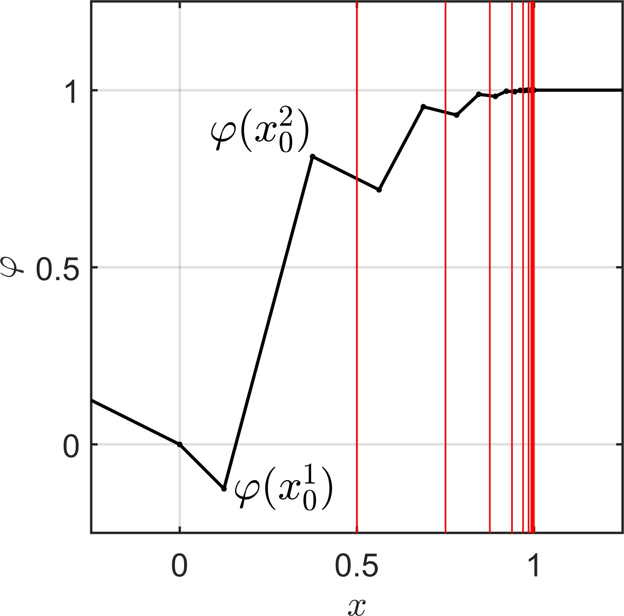
Then xi1<xi2<xi+11superscriptsubscriptπ‘₯𝑖1superscriptsubscriptπ‘₯𝑖2superscriptsubscriptπ‘₯𝑖11x_{i}^{1}<x_{i}^{2}<x_{i+1}^{1} for all iβˆˆβ„•βˆͺ{0}𝑖ℕ0i\in\mathbb{N}\cup\{0\}. We construct a function Ο†:ℝ→ℝ:πœ‘β†’β„β„\varphi:\mathbb{R}\rightarrow\mathbb{R} as follows: For x<0π‘₯0x<0 let φ​(x):=βˆ’12​xassignπœ‘π‘₯12π‘₯\varphi(x):=-\frac{1}{2}x, for xβ‰₯1π‘₯1x\geq 1 let φ​(x):=1assignπœ‘π‘₯1\varphi(x):=1 and on [0,1)01[0,1) let Ο†πœ‘\varphi be the piecewise linear function with φ​(0)=0πœ‘00\varphi(0)=0 and

φ​(xi1)=Ο†i1andφ​(xi2)=Ο†i2βˆ€iβˆˆβ„•βˆͺ{0}.formulae-sequenceπœ‘superscriptsubscriptπ‘₯𝑖1superscriptsubscriptπœ‘π‘–1andformulae-sequenceπœ‘superscriptsubscriptπ‘₯𝑖2superscriptsubscriptπœ‘π‘–2for-all𝑖ℕ0\displaystyle\varphi(x_{i}^{1})=\varphi_{i}^{1}\quad\text{and}\quad\varphi(x_{i}^{2})=\varphi_{i}^{2}\quad\forall i\in\mathbb{N}\cup\{0\}.

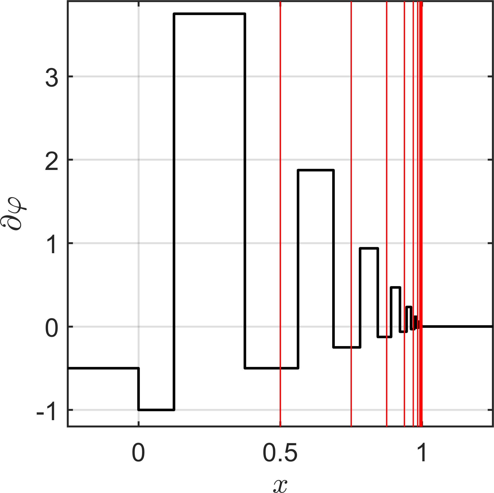
The graph of Ο†πœ‘\varphi is shown in Figure 1(a). Figure 1(b) shows the gradient of Ο†πœ‘\varphi at points where Ο†πœ‘\varphi is differentiable, and a vertical line from smallest to the largest subgradient at points where Ο†πœ‘\varphi is not differentiable.

Refer to caption

(a)

Refer to caption

(b)

Refer to caption

(c)

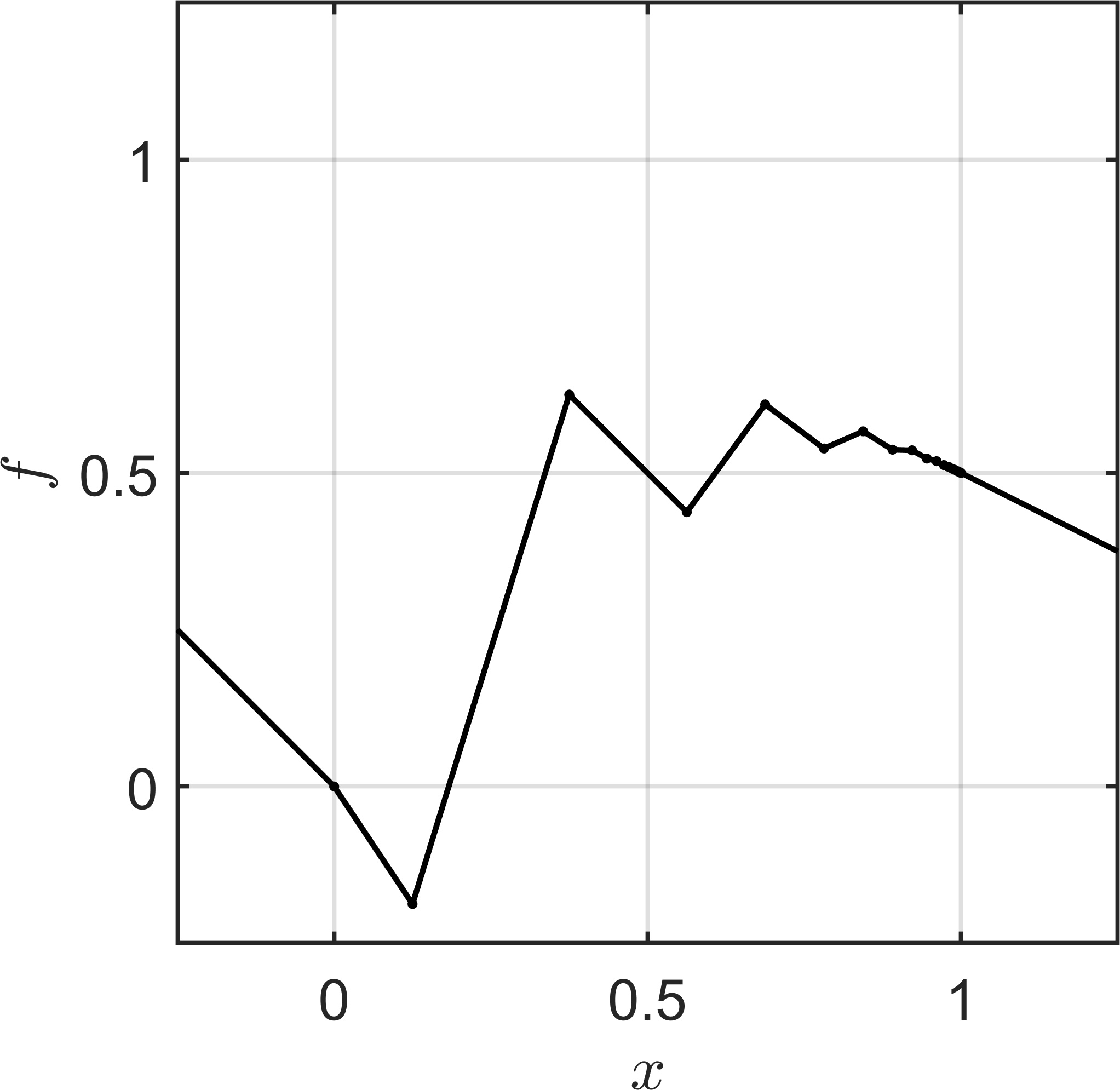
Figure 1: The graphs of (a) Ο†=hπœ‘β„Ž\varphi=h, (b) βˆ‚Ο†=βˆ‚hπœ‘β„Ž\partial\varphi=\partial h and (c) f𝑓f in Example 1. The red lines show the values of tj=1βˆ’2βˆ’jsubscript𝑑𝑗1superscript2𝑗t_{j}=1-2^{-j} for jβˆˆβ„•π‘—β„•j\in\mathbb{N}.

We see that in the limit xβ†’1β†’π‘₯1x\rightarrow 1, all subgradients tend to 00. Based on this observation, it can be shown that Ο†πœ‘\varphi is semismooth.
Now let

f:ℝ→ℝ,x↦φ​(x)βˆ’12​x:𝑓formulae-sequence→ℝℝmaps-toπ‘₯πœ‘π‘₯12π‘₯\displaystyle f:\mathbb{R}\rightarrow\mathbb{R},\quad x\mapsto\varphi(x)-\frac{1}{2}x

as shown in Figure 1(c). Let x0=0subscriptπ‘₯00x_{0}=0, Ξ΅=1πœ€1\varepsilon=1 and c=1/2𝑐12c=1/2. Assume that we have evaluated the subgradient ΞΎ:=βˆ’1βˆˆβˆ‚f​(0)=[βˆ’3/2,βˆ’1]assignπœ‰1𝑓0321\xi:=-1\in\partial f(0)=[-3/2,-1]. Then for W={ΞΎ}π‘Šπœ‰W=\{\xi\}, the direction v~~𝑣\tilde{v} from (7) is simply v~=βˆ’ΞΎ=1~π‘£πœ‰1\tilde{v}=-\xi=1. When checking whether v~~𝑣\tilde{v} yields sufficient decrease, we see that

f​(x0+Ξ΅β€–v~‖​v~)βˆ’f​(x0)=f​(1)βˆ’f​(0)=12>βˆ’12=βˆ’c​Ρ​‖v~β€–,𝑓subscriptπ‘₯0πœ€norm~𝑣~𝑣𝑓subscriptπ‘₯0𝑓1𝑓01212π‘πœ€norm~𝑣\displaystyle f\left(x_{0}+\frac{\varepsilon}{\|\tilde{v}\|}\tilde{v}\right)-f(x_{0})=f\left(1\right)-f(0)=\frac{1}{2}>-\frac{1}{2}=-c\varepsilon\|\tilde{v}\|,

i.e., v~~𝑣\tilde{v} does not yield sufficient (or even any) decrease.
For Algorithm 1 we have

h​(t)=f​(x0+t​v~)βˆ’f​(x0)+c​t​‖v~β€–2=f​(t)+12​t=φ​(t).β„Žπ‘‘π‘“subscriptπ‘₯0𝑑~𝑣𝑓subscriptπ‘₯0𝑐𝑑superscriptnorm~𝑣2𝑓𝑑12π‘‘πœ‘π‘‘\displaystyle h(t)=f(x_{0}+t\tilde{v})-f(x_{0})+ct\|\tilde{v}\|^{2}=f(t)+\frac{1}{2}t=\varphi(t).

Since 1=h​(1)=h​(b1)>h​(t)1β„Ž1β„Žsubscript𝑏1β„Žπ‘‘1=h(1)=h(b_{1})>h(t) for all t∈[0,1)𝑑01t\in[0,1), we have

aj=1βˆ’2βˆ’j+1,bj=1,tj=1βˆ’2βˆ’jβˆ€jβˆˆβ„•,formulae-sequencesubscriptπ‘Žπ‘—1superscript2𝑗1formulae-sequencesubscript𝑏𝑗1formulae-sequencesubscript𝑑𝑗1superscript2𝑗for-all𝑗ℕ\displaystyle a_{j}=1-2^{-j+1},\ b_{j}=1,\ t_{j}=1-2^{-j}\quad\forall j\in\mathbb{N},

as indicated in Figure 1(a) and (b). By construction (cf. Figure 1(b)), f𝑓f is continuously differentiable at all x0+tj​v~=tjsubscriptπ‘₯0subscript𝑑𝑗~𝑣subscript𝑑𝑗x_{0}+t_{j}\tilde{v}=t_{j} and

βˆ‚f​(x0+tj​v~)={βˆ‡f​(tj)}={βˆ’2βˆ’jβˆ’12}βˆ€jβˆˆβ„•,formulae-sequence𝑓subscriptπ‘₯0subscript𝑑𝑗~π‘£βˆ‡π‘“subscript𝑑𝑗superscript2𝑗12for-all𝑗ℕ\displaystyle\partial f(x_{0}+t_{j}\tilde{v})=\{\nabla f(t_{j})\}=\left\{-2^{-j}-\frac{1}{2}\right\}\quad\forall j\in\mathbb{N},

so

βŸ¨ΞΎβ€²,v~⟩=βˆ’2βˆ’jβˆ’12<βˆ’12=βˆ’c​‖v~β€–2βˆ€jβˆˆβ„•.formulae-sequencesuperscriptπœ‰β€²~𝑣superscript2𝑗1212𝑐superscriptnorm~𝑣2for-all𝑗ℕ\displaystyle\langle\xi^{\prime},\tilde{v}\rangle=-2^{-j}-\frac{1}{2}<-\frac{1}{2}=-c\|\tilde{v}\|^{2}\quad\forall j\in\mathbb{N}.

Thus, Algorithm 1 does not terminate.

Note that in the previous example, only the nonsmoothness of f𝑓f at x=1π‘₯1x=1 is relevant for the failure of the algorithm. Thus, by β€œsmoothing” the objective f𝑓f at all kinks except 111, one could even construct a semismooth function which is continuously differentiable everywhere outside of a single point for which the algorithm fails.

3 Improved bisection method

In this section, we propose a slightly modified version of Algorithm 1 and prove termination for the case where the objective f𝑓f is weakly lower semismooth. For any xβˆˆβ„nπ‘₯superscriptℝ𝑛x\in\mathbb{R}^{n}, we assume that we are only able to evaluate a single, arbitrary subgradient of the locally Lipschitz continuous f𝑓f at xπ‘₯x.

3.1 Derivation of the improved method

Roughly speaking, the idea is to use a smaller parameter c~<c~𝑐𝑐\tilde{c}<c in hβ„Žh (cf. (10)) to try to find a new subgradient that satisfies a stricter version of inequality (2.2). This will solve the first of the issues described in Section 2.2, as even points in which βˆ‚hβ„Ž\partial h is negative but close to zero then suffice to find subgradients that satisfy the weaker requirement with respect to c𝑐c.

More precisely, note that v~~𝑣\tilde{v} is an unacceptable descent direction if and only if

f​(x0+Ξ΅β€–v~‖​v~)>f​(x0)βˆ’c​Ρ​‖v~‖𝑓subscriptπ‘₯0πœ€norm~𝑣~𝑣𝑓subscriptπ‘₯0π‘πœ€norm~𝑣\displaystyle f\left(x_{0}+\frac{\varepsilon}{\|\tilde{v}\|}\tilde{v}\right)>f(x_{0})-c\varepsilon\|\tilde{v}\|
⇔⇔\displaystyle\Leftrightarrow\quad cmin:=βˆ’f​(x0+Ξ΅β€–v~‖​v~)βˆ’f​(x0)Ρ​‖v~β€–<c.assignsubscript𝑐min𝑓subscriptπ‘₯0πœ€norm~𝑣~𝑣𝑓subscriptπ‘₯0πœ€norm~𝑣𝑐\displaystyle c_{\text{min}}:=-\frac{f\left(x_{0}+\frac{\varepsilon}{\|\tilde{v}\|}\tilde{v}\right)-f(x_{0})}{\varepsilon\|\tilde{v}\|}<c.

Thus, if v~~𝑣\tilde{v} is an unacceptable direction, then it is also unacceptable if we replace c𝑐c in (8) by any c~∈(cmin,c)β‰ βˆ…~𝑐subscript𝑐min𝑐\tilde{c}\in(c_{\text{min}},c)\neq\emptyset. In other words, we could apply Algorithm 1 for any c~∈(cmin,c)~𝑐subscript𝑐min𝑐\tilde{c}\in(c_{\text{min}},c) and the method would still produce sequences with hc~​(aj)<hc~​(bj)subscriptβ„Ž~𝑐subscriptπ‘Žπ‘—subscriptβ„Ž~𝑐subscript𝑏𝑗h_{\tilde{c}}(a_{j})<h_{\tilde{c}}(b_{j}) for all jβˆˆβ„•π‘—β„•j\in\mathbb{N}, where, analogously to (10),

hc~:ℝ→ℝ,t↦f​(x0+t​v~)βˆ’f​(x0)+c~​t​‖v~β€–2.:subscriptβ„Ž~𝑐formulae-sequence→ℝℝmaps-to𝑑𝑓subscriptπ‘₯0𝑑~𝑣𝑓subscriptπ‘₯0~𝑐𝑑superscriptnorm~𝑣2\displaystyle h_{\tilde{c}}:\mathbb{R}\rightarrow\mathbb{R},\quad t\mapsto f(x_{0}+t\tilde{v})-f(x_{0})+\tilde{c}t\|\tilde{v}\|^{2}.

In step 333, the method would check whether βŸ¨ΞΎβ€²,v~⟩>βˆ’c~​‖v~β€–2superscriptπœ‰β€²~𝑣~𝑐superscriptnorm~𝑣2\langle\xi^{\prime},\tilde{v}\rangle>-\tilde{c}\|\tilde{v}\|^{2}. But since c~<c~𝑐𝑐\tilde{c}<c, this inequality is stricter than (2.2). Thus, instead, we apply Algorithm 1 with only hβ„Žh being replaced by hc~subscriptβ„Ž~𝑐h_{\tilde{c}} and the rest unchanged. In terms of the subdifferential of hc~subscriptβ„Ž~𝑐h_{\tilde{c}}, this means that the method may stop as soon as

βˆƒgβˆˆβˆ‚hc~​(tj):g=βŸ¨ΞΎβ€²,v~⟩+c~​‖v~β€–2>(c~βˆ’c)​‖v~β€–2,:𝑔subscriptβ„Ž~𝑐subscript𝑑𝑗𝑔superscriptπœ‰β€²~𝑣~𝑐superscriptnorm~𝑣2~𝑐𝑐superscriptnorm~𝑣2\displaystyle\exists g\in\partial h_{\tilde{c}}(t_{j}):g=\langle\xi^{\prime},\tilde{v}\rangle+\tilde{c}\|\tilde{v}\|^{2}>(\tilde{c}-c)\|\tilde{v}\|^{2}, (12)

where (c~βˆ’c)​‖v~β€–2<0~𝑐𝑐superscriptnorm~𝑣20(\tilde{c}-c)\|\tilde{v}\|^{2}<0. For clarity, this modified algorithm is denoted in Algorithm 2.

Algorithm 2 Improved computation of new Ξ΅πœ€\varepsilon-subgradients
1:Point x0βˆˆβ„nsubscriptπ‘₯0superscriptℝ𝑛x_{0}\in\mathbb{R}^{n}, radius Ξ΅>0πœ€0\varepsilon>0, descent parameters c∈(0,1)𝑐01c\in(0,1), c~∈(cmin,c)~𝑐subscript𝑐min𝑐\tilde{c}\in(c_{\text{min}},c), direction v~βˆˆβ„nβˆ–{0}~𝑣superscriptℝ𝑛0\tilde{v}\in\mathbb{R}^{n}\setminus\{0\} violating (8).
2:Initialize j=1𝑗1j=1, a1=0subscriptπ‘Ž10a_{1}=0, b1=Ξ΅β€–v~β€–subscript𝑏1πœ€norm~𝑣b_{1}=\frac{\varepsilon}{\|\tilde{v}\|} and t1=12​(a1+b1)subscript𝑑112subscriptπ‘Ž1subscript𝑏1t_{1}=\frac{1}{2}(a_{1}+b_{1}).
3:Compute ΞΎβ€²βˆˆβˆ‚f​(x0+tj​v~)superscriptπœ‰β€²π‘“subscriptπ‘₯0subscript𝑑𝑗~𝑣\xi^{\prime}\in\partial f(x_{0}+t_{j}\tilde{v}).
4:If βŸ¨ΞΎβ€²,v~⟩>βˆ’c​‖v~β€–2superscriptπœ‰β€²~𝑣𝑐superscriptnorm~𝑣2\langle\xi^{\prime},\tilde{v}\rangle>-c\|\tilde{v}\|^{2} then stop.
5:If hc~​(bj)>hc~​(tj)subscriptβ„Ž~𝑐subscript𝑏𝑗subscriptβ„Ž~𝑐subscript𝑑𝑗h_{\tilde{c}}(b_{j})>h_{\tilde{c}}(t_{j}) then set aj+1=tjsubscriptπ‘Žπ‘—1subscript𝑑𝑗a_{j+1}=t_{j} and bj+1=bjsubscript𝑏𝑗1subscript𝑏𝑗b_{j+1}=b_{j}. Otherwise set aj+1=ajsubscriptπ‘Žπ‘—1subscriptπ‘Žπ‘—a_{j+1}=a_{j} and bj+1=tjsubscript𝑏𝑗1subscript𝑑𝑗b_{j+1}=t_{j}.
6:Set tj+1=12​(aj+1+bj+1)subscript𝑑𝑗112subscriptπ‘Žπ‘—1subscript𝑏𝑗1t_{j+1}=\frac{1}{2}(a_{j+1}+b_{j+1}), j=j+1𝑗𝑗1j=j+1 and go to step 2.

3.2 Proof of termination

We begin the analysis of Algorithm 2 with some simple, technical results.

Lemma 1.

If Algorithm 2 does not terminate, then

  1. (i)

    (aj)jsubscriptsubscriptπ‘Žπ‘—π‘—(a_{j})_{j}, (bj)jsubscriptsubscript𝑏𝑗𝑗(b_{j})_{j} and (tj)jsubscriptsubscript𝑑𝑗𝑗(t_{j})_{j} have the same limit t¯∈[0,Ξ΅/β€–v~β€–]¯𝑑0πœ€norm~𝑣\bar{t}\in[0,\varepsilon/\|\tilde{v}\|],

  2. (ii)

    t¯∈[aj,bj]¯𝑑subscriptπ‘Žπ‘—subscript𝑏𝑗\bar{t}\in[a_{j},b_{j}] for all jβˆˆβ„•π‘—β„•j\in\mathbb{N},

  3. (iii)

    (hc~​(bj))jsubscriptsubscriptβ„Ž~𝑐subscript𝑏𝑗𝑗(h_{\tilde{c}}(b_{j}))_{j} is monotonically increasing and hc~​(aj)<hc~​(bj)subscriptβ„Ž~𝑐subscriptπ‘Žπ‘—subscriptβ„Ž~𝑐subscript𝑏𝑗h_{\tilde{c}}(a_{j})<h_{\tilde{c}}(b_{j}) for all jβˆˆβ„•π‘—β„•j\in\mathbb{N},

  4. (iv)

    tj<tΒ―subscript𝑑𝑗¯𝑑t_{j}<\bar{t} for infinitely many jβˆˆβ„•π‘—β„•j\in\mathbb{N}.

Proof 3.1.

(i) By construction (aj)jsubscriptsubscriptπ‘Žπ‘—π‘—(a_{j})_{j} is monotonically increasing and (bj)jsubscriptsubscript𝑏𝑗𝑗(b_{j})_{j} is monotonically decreasing in [0,Ξ΅/β€–v~β€–]0πœ€norm~𝑣[0,\varepsilon/\|\tilde{v}\|], so both sequences converge. Since Algorithm 2 does not terminate, it holds limjβ†’βˆžbjβˆ’aj=0subscript→𝑗subscript𝑏𝑗subscriptπ‘Žπ‘—0\lim_{j\rightarrow\infty}b_{j}-a_{j}=0, so they must converge to the same limit t¯∈[0,Ξ΅/β€–v~β€–]¯𝑑0πœ€norm~𝑣\bar{t}\in[0,\varepsilon/\|\tilde{v}\|]. Since tj∈(aj,bj)subscript𝑑𝑗subscriptπ‘Žπ‘—subscript𝑏𝑗t_{j}\in(a_{j},b_{j}) for all jβˆˆβ„•π‘—β„•j\in\mathbb{N}, (tj)jsubscriptsubscript𝑑𝑗𝑗(t_{j})_{j} must have the same limit.
(ii) Assume that tΒ―βˆ‰[aj,bj]¯𝑑subscriptπ‘Žπ‘—subscript𝑏𝑗\bar{t}\notin[a_{j},b_{j}] for some jβˆˆβ„•π‘—β„•j\in\mathbb{N}. Then either tΒ―<aj¯𝑑subscriptπ‘Žπ‘—\bar{t}<a_{j} or tΒ―>bj¯𝑑subscript𝑏𝑗\bar{t}>b_{j}. Due to the monotonicity of (aj)jsubscriptsubscriptπ‘Žπ‘—π‘—(a_{j})_{j} and (bj)jsubscriptsubscript𝑏𝑗𝑗(b_{j})_{j}, this is a contradiction to t¯¯𝑑\bar{t} being the limit of both sequences.
(iii) By construction, the value of (bj)jsubscriptsubscript𝑏𝑗𝑗(b_{j})_{j} only changes when hc~​(bj)≀hc~​(tj)subscriptβ„Ž~𝑐subscript𝑏𝑗subscriptβ„Ž~𝑐subscript𝑑𝑗h_{\tilde{c}}(b_{j})\leq h_{\tilde{c}}(t_{j}) in step 4. In this case bj+1subscript𝑏𝑗1b_{j+1} is set to tjsubscript𝑑𝑗t_{j}, so we have hc~​(bj+1)=hc~​(tj)β‰₯hc~​(bj)subscriptβ„Ž~𝑐subscript𝑏𝑗1subscriptβ„Ž~𝑐subscript𝑑𝑗subscriptβ„Ž~𝑐subscript𝑏𝑗h_{\tilde{c}}(b_{j+1})=h_{\tilde{c}}(t_{j})\geq h_{\tilde{c}}(b_{j}) and hc~​(aj+1)=hc~​(aj)subscriptβ„Ž~𝑐subscriptπ‘Žπ‘—1subscriptβ„Ž~𝑐subscriptπ‘Žπ‘—h_{\tilde{c}}(a_{j+1})=h_{\tilde{c}}(a_{j}). If, on the other hand, hc~​(bj)>hc~​(tj)subscriptβ„Ž~𝑐subscript𝑏𝑗subscriptβ„Ž~𝑐subscript𝑑𝑗h_{\tilde{c}}(b_{j})>h_{\tilde{c}}(t_{j}), then aj+1=tjsubscriptπ‘Žπ‘—1subscript𝑑𝑗a_{j+1}=t_{j}, so hc~​(aj+1)=hc~​(tj)<hc~​(bj)=hc~​(bj+1)subscriptβ„Ž~𝑐subscriptπ‘Žπ‘—1subscriptβ„Ž~𝑐subscript𝑑𝑗subscriptβ„Ž~𝑐subscript𝑏𝑗subscriptβ„Ž~𝑐subscript𝑏𝑗1h_{\tilde{c}}(a_{j+1})=h_{\tilde{c}}(t_{j})<h_{\tilde{c}}(b_{j})=h_{\tilde{c}}(b_{j+1}). The proof follows by induction.
(iv) Assume that this does not hold. Then there is some Nβˆˆβ„•π‘β„•N\in\mathbb{N} such that tjβ‰₯tΒ―subscript𝑑𝑗¯𝑑t_{j}\geq\bar{t} for all j>N𝑗𝑁j>N. By construction of (tj)jsubscriptsubscript𝑑𝑗𝑗(t_{j})_{j}, tj=tΒ―subscript𝑑𝑗¯𝑑t_{j}=\bar{t} may only hold once, so we can assume w.l.o.g. that tj>tΒ―subscript𝑑𝑗¯𝑑t_{j}>\bar{t} for all j>N𝑗𝑁j>N. Since t¯∈[aj,bj]¯𝑑subscriptπ‘Žπ‘—subscript𝑏𝑗\bar{t}\in[a_{j},b_{j}] for all jβˆˆβ„•π‘—β„•j\in\mathbb{N} and tjsubscript𝑑𝑗t_{j} is the midpoint of [aj,bj]subscriptπ‘Žπ‘—subscript𝑏𝑗[a_{j},b_{j}], this implies that aj=aNsubscriptπ‘Žπ‘—subscriptπ‘Žπ‘a_{j}=a_{N} for all j>N𝑗𝑁j>N. In particular, tΒ―=limjβ†’βˆžaj=aN¯𝑑subscript→𝑗subscriptπ‘Žπ‘—subscriptπ‘Žπ‘\bar{t}=\lim_{j\rightarrow\infty}a_{j}=a_{N}. Since hc~​(tΒ―)=hc~​(aN)<hc~​(bN)subscriptβ„Ž~𝑐¯𝑑subscriptβ„Ž~𝑐subscriptπ‘Žπ‘subscriptβ„Ž~𝑐subscript𝑏𝑁h_{\tilde{c}}(\bar{t})=h_{\tilde{c}}(a_{N})<h_{\tilde{c}}(b_{N}) and (hc~​(bj))jsubscriptsubscriptβ„Ž~𝑐subscript𝑏𝑗𝑗(h_{\tilde{c}}(b_{j}))_{j} is monotonically increasing with limjβ†’βˆžhc~​(bj)=hc~​(tΒ―)subscript→𝑗subscriptβ„Ž~𝑐subscript𝑏𝑗subscriptβ„Ž~𝑐¯𝑑\lim_{j\rightarrow\infty}h_{\tilde{c}}(b_{j})=h_{\tilde{c}}(\bar{t}) due to continuity, this is a contradiction.

To be able to fix the second of the two issues mentioned in Section 2.2, we need a stronger assumption for f𝑓f. An easy way to solve the issue would be to force equality in the chain rule (11) by assuming that f𝑓f is regular (cf. [1], Definition 2.3.4). While the class of regular functions includes convex functions, even simple nonconvex functions like xβ†¦βˆ’|x|maps-toπ‘₯π‘₯x\mapsto-|x| are not regular. As such, this assumption would heavily restrict the applicability of the method. Fortunately, we do not actually need equality in (11) as we are only interested in the behavior of βŸ¨βˆ‚f​(x0+t​v~),v~βŸ©π‘“subscriptπ‘₯0𝑑~𝑣~𝑣\langle\partial f(x_{0}+t\tilde{v}),\tilde{v}\rangle for tβ†’t¯→𝑑¯𝑑t\rightarrow\bar{t}, and not necessarily in βŸ¨βˆ‚f​(x0+t¯​v~),v~βŸ©π‘“subscriptπ‘₯0¯𝑑~𝑣~𝑣\langle\partial f(x_{0}+\bar{t}\tilde{v}),\tilde{v}\rangle itself. Thus, we will see that it suffices to assume that f𝑓f is weakly lower semismooth [9, 10], which means that it is locally Lipschitz and for xβˆˆβ„nπ‘₯superscriptℝ𝑛x\in\mathbb{R}^{n}, vβˆˆβ„n𝑣superscriptℝ𝑛v\in\mathbb{R}^{n} and sequences (si)iβˆˆβ„>0subscriptsubscript𝑠𝑖𝑖superscriptℝabsent0(s_{i})_{i}\in\mathbb{R}^{>0}, (ΞΎi)iβˆˆβ„nsubscriptsubscriptπœ‰π‘–π‘–superscriptℝ𝑛(\xi_{i})_{i}\in\mathbb{R}^{n} with siβ†˜0β†˜subscript𝑠𝑖0s_{i}\searrow 0 and ΞΎiβˆˆβˆ‚f​(x+si​v)subscriptπœ‰π‘–π‘“π‘₯subscript𝑠𝑖𝑣\xi_{i}\in\partial f(x+s_{i}v) for all iβˆˆβ„•π‘–β„•i\in\mathbb{N}, it holds

lim supiβ†’βˆžβŸ¨ΞΎi,vβŸ©β‰€lim infsβ†˜0f​(x+s​v)βˆ’f​(x)s.subscriptlimit-supremum→𝑖subscriptπœ‰π‘–π‘£subscriptlimit-infimumβ†˜π‘ 0𝑓π‘₯𝑠𝑣𝑓π‘₯𝑠\displaystyle\limsup_{i\rightarrow\infty}\ \langle\xi_{i},v\rangle\leq\liminf_{s\searrow 0}\frac{f(x+sv)-f(x)}{s}. (13)

Roughly speaking, weak lower semismoothness means that there is a semicontinuous relationship between directional derivatives and sequences of subgradients (via the inner product). In our case, we are interested in inequality (13) for x=x0+t¯​v~π‘₯subscriptπ‘₯0¯𝑑~𝑣x=x_{0}+\bar{t}\tilde{v} and v=βˆ’v~𝑣~𝑣v=-\tilde{v}. This will give us a lower estimate for βŸ¨ΞΎβ€²,v~⟩superscriptπœ‰β€²~𝑣\langle\xi^{\prime},\tilde{v}\rangle in step 3 of Algorithm 2, which we can use to show termination.

To this end, we will first derive an upper bound for the right-hand side of (13) in the following lemma.

Lemma 3.2.

Assume that Algorithm 2 does not terminate. Let t¯¯𝑑\bar{t} as in Lemma 1. Then

lim infsβ†˜0f​(x0+t¯​v~βˆ’s​v~)βˆ’f​(x0+t¯​v~)s≀c~​‖v~β€–2.subscriptlimit-infimumβ†˜π‘ 0𝑓subscriptπ‘₯0¯𝑑~𝑣𝑠~𝑣𝑓subscriptπ‘₯0¯𝑑~𝑣𝑠~𝑐superscriptnorm~𝑣2\displaystyle\liminf_{s\searrow 0}\frac{f(x_{0}+\bar{t}\tilde{v}-s\tilde{v})-f(x_{0}+\bar{t}\tilde{v})}{s}\leq\tilde{c}\|\tilde{v}\|^{2}. (14)
Proof 3.3.

By Lemma 1 we have tj<tΒ―subscript𝑑𝑗¯𝑑t_{j}<\bar{t} for infinitely many jβˆˆβ„•π‘—β„•j\in\mathbb{N}. Let (ji)isubscriptsubscript𝑗𝑖𝑖(j_{i})_{i} be the sequence of such j𝑗j. Note that monotonicity of (hc~​(bj))jsubscriptsubscriptβ„Ž~𝑐subscript𝑏𝑗𝑗(h_{\tilde{c}}(b_{j}))_{j} and tji<tΒ―subscript𝑑subscript𝑗𝑖¯𝑑t_{j_{i}}<\bar{t} imply that

hc~​(tΒ―)=limjβ†’βˆžhc~​(bj)β‰₯hc~​(bji)>hc~​(tji)βˆ€iβˆˆβ„•.formulae-sequencesubscriptβ„Ž~𝑐¯𝑑subscript→𝑗subscriptβ„Ž~𝑐subscript𝑏𝑗subscriptβ„Ž~𝑐subscript𝑏subscript𝑗𝑖subscriptβ„Ž~𝑐subscript𝑑subscript𝑗𝑖for-all𝑖ℕ\displaystyle h_{\tilde{c}}(\bar{t})=\lim_{j\rightarrow\infty}h_{\tilde{c}}(b_{j})\geq h_{\tilde{c}}(b_{j_{i}})>h_{\tilde{c}}(t_{j_{i}})\quad\forall i\in\mathbb{N}.

In particular, writing f​(x0+tji​v~)=f​(x0+t¯​v~βˆ’(tΒ―βˆ’tji)​v~)𝑓subscriptπ‘₯0subscript𝑑subscript𝑗𝑖~𝑣𝑓subscriptπ‘₯0¯𝑑~𝑣¯𝑑subscript𝑑subscript𝑗𝑖~𝑣f(x_{0}+t_{j_{i}}\tilde{v})=f(x_{0}+\bar{t}\tilde{v}-(\bar{t}-t_{j_{i}})\tilde{v}), it holds

0>hc~​(tji)βˆ’hc~​(tΒ―)=f​(x0+t¯​v~βˆ’(tΒ―βˆ’tji)​v~)βˆ’f​(x0+t¯​v~)+c~​(tjiβˆ’tΒ―)​‖v~β€–20subscriptβ„Ž~𝑐subscript𝑑subscript𝑗𝑖subscriptβ„Ž~𝑐¯𝑑𝑓subscriptπ‘₯0¯𝑑~𝑣¯𝑑subscript𝑑subscript𝑗𝑖~𝑣𝑓subscriptπ‘₯0¯𝑑~𝑣~𝑐subscript𝑑subscript𝑗𝑖¯𝑑superscriptnorm~𝑣2\displaystyle 0>h_{\tilde{c}}(t_{j_{i}})-h_{\tilde{c}}(\bar{t})=f(x_{0}+\bar{t}\tilde{v}-(\bar{t}-t_{j_{i}})\tilde{v})-f(x_{0}+\bar{t}\tilde{v})+\tilde{c}(t_{j_{i}}-\bar{t})\|\tilde{v}\|^{2}
⇔⇔\displaystyle\Leftrightarrow\quad f​(x0+t¯​v~βˆ’(tΒ―βˆ’tji)​v~)βˆ’f​(x0+t¯​v~)tΒ―βˆ’tji<c~​‖v~β€–2𝑓subscriptπ‘₯0¯𝑑~𝑣¯𝑑subscript𝑑subscript𝑗𝑖~𝑣𝑓subscriptπ‘₯0¯𝑑~𝑣¯𝑑subscript𝑑subscript𝑗𝑖~𝑐superscriptnorm~𝑣2\displaystyle\frac{f(x_{0}+\bar{t}\tilde{v}-(\bar{t}-t_{j_{i}})\tilde{v})-f(x_{0}+\bar{t}\tilde{v})}{\bar{t}-t_{j_{i}}}<\tilde{c}\|\tilde{v}\|^{2}

for all iβˆˆβ„•π‘–β„•i\in\mathbb{N}. Since tΒ―βˆ’tjiβ†˜0β†˜Β―π‘‘subscript𝑑subscript𝑗𝑖0\bar{t}-t_{j_{i}}\searrow 0 and the limit inferior is taken in (14), this completes the proof.

The previous lemma enables us to prove our main result.

Theorem 3.4.

Assume that f𝑓f is weakly lower semismooth. Then Algorithm 2 terminates.

Proof 3.5.

Assume that Algorithm 2 does not terminate. Choose (ji)isubscriptsubscript𝑗𝑖𝑖(j_{i})_{i} as in the proof of Lemma 3.2 and let ΞΎiβ€²βˆˆβˆ‚f​(x0+tji​v~)subscriptsuperscriptπœ‰β€²π‘–π‘“subscriptπ‘₯0subscript𝑑subscript𝑗𝑖~𝑣\xi^{\prime}_{i}\in\partial f(x_{0}+t_{j_{i}}\tilde{v}) be the subgradient evaluated in step 3 in iteration jisubscript𝑗𝑖j_{i}. Let si:=tΒ―βˆ’tjiassignsubscript𝑠𝑖¯𝑑subscript𝑑subscript𝑗𝑖s_{i}:=\bar{t}-t_{j_{i}}. Then ΞΎiβ€²βˆˆβˆ‚f​(x0+tji​v~)=βˆ‚f​(x0+t¯​v~βˆ’si​v~)subscriptsuperscriptπœ‰β€²π‘–π‘“subscriptπ‘₯0subscript𝑑subscript𝑗𝑖~𝑣𝑓subscriptπ‘₯0¯𝑑~𝑣subscript𝑠𝑖~𝑣\xi^{\prime}_{i}\in\partial f(x_{0}+t_{j_{i}}\tilde{v})=\partial f(x_{0}+\bar{t}\tilde{v}-s_{i}\tilde{v}) and siβ†˜0β†˜subscript𝑠𝑖0s_{i}\searrow 0, so by Lemma 3.2 and weak lower semismoothness, it holds

lim infiβ†’βˆžβŸ¨ΞΎiβ€²,v~⟩subscriptlimit-infimum→𝑖subscriptsuperscriptπœ‰β€²π‘–~𝑣\displaystyle\liminf_{i\rightarrow\infty}\ \langle\xi^{\prime}_{i},\tilde{v}\rangle =βˆ’lim supiβ†’βˆžβŸ¨ΞΎiβ€²,βˆ’v~⟩β‰₯βˆ’lim infsβ†˜0f​(x0+t¯​v~βˆ’s​v~)βˆ’f​(x0+t¯​v~)sabsentsubscriptlimit-supremum→𝑖subscriptsuperscriptπœ‰β€²π‘–~𝑣subscriptlimit-infimumβ†˜π‘ 0𝑓subscriptπ‘₯0¯𝑑~𝑣𝑠~𝑣𝑓subscriptπ‘₯0¯𝑑~𝑣𝑠\displaystyle=-\limsup_{i\rightarrow\infty}\ \langle\xi^{\prime}_{i},-\tilde{v}\rangle\geq-\liminf_{s\searrow 0}\frac{f(x_{0}+\bar{t}\tilde{v}-s\tilde{v})-f(x_{0}+\bar{t}\tilde{v})}{s}
β‰₯βˆ’c~​‖v~β€–2>βˆ’c​‖v~β€–2,absent~𝑐superscriptnorm~𝑣2𝑐superscriptnorm~𝑣2\displaystyle\geq-\tilde{c}\|\tilde{v}\|^{2}>-c\|\tilde{v}\|^{2},

since c~∈(cmin,c)~𝑐subscript𝑐min𝑐\tilde{c}\in(c_{\text{min}},c). In particular, we must have

⟨ξiβ€²,v~⟩>βˆ’c​‖v~β€–2subscriptsuperscriptπœ‰β€²π‘–~𝑣𝑐superscriptnorm~𝑣2\displaystyle\langle\xi^{\prime}_{i},\tilde{v}\rangle>-c\|\tilde{v}\|^{2}

after finitely many iterations, causing the algorithm to stop in step 333.

4 Example

In this section, we visualize the difference between Algorithms 1 and 2 by revisiting Example 1.

Example 4.6.
  1. (a)

    In the situation of Example 1, it holds

    cmin=βˆ’f​(0+1)βˆ’f​(0)1=βˆ’12,subscript𝑐min𝑓01𝑓0112\displaystyle c_{\text{min}}=-\frac{f(0+1)-f(0)}{1}=-\frac{1}{2},

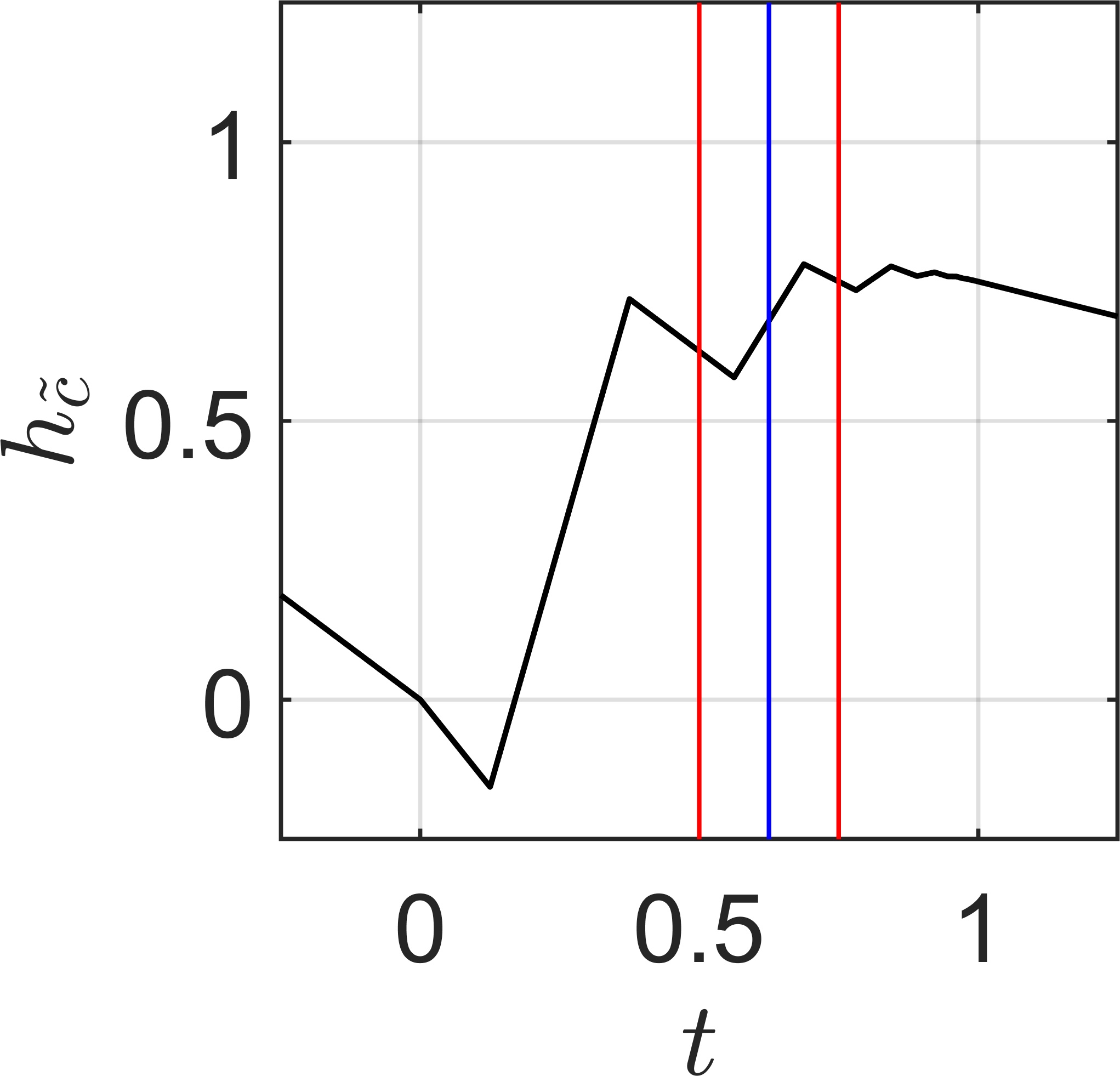
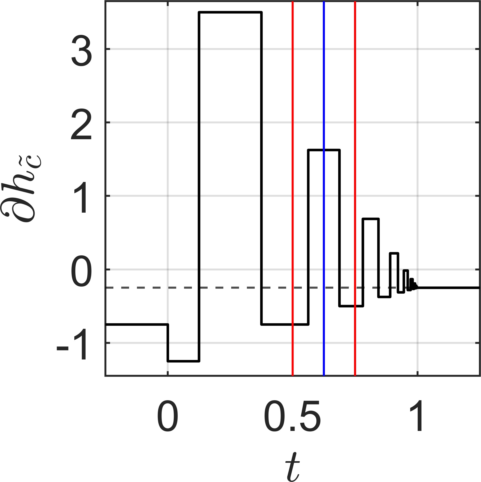
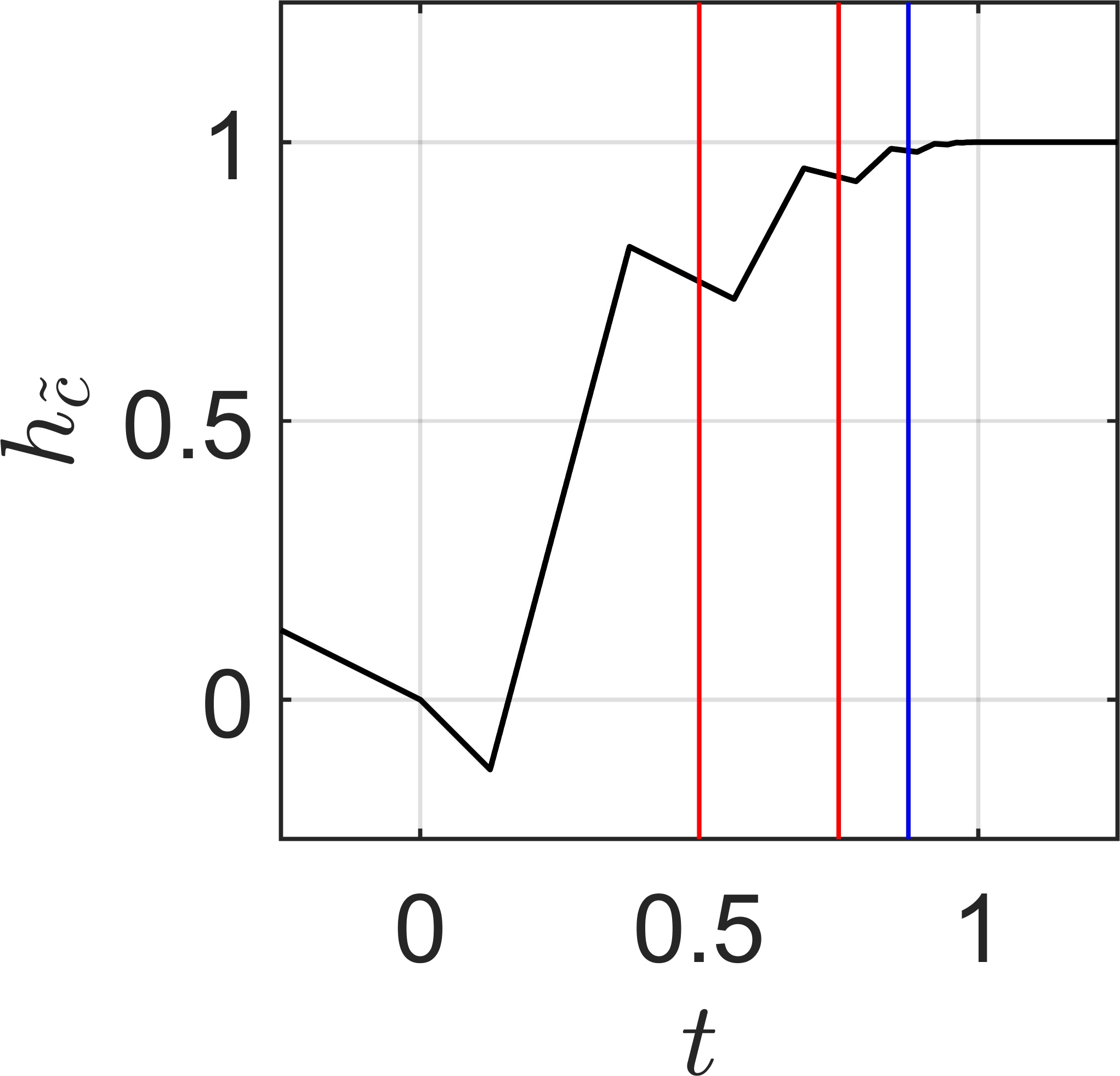
    so any c~∈(βˆ’1/2,c)=(βˆ’1/2,1/2)~𝑐12𝑐1212\tilde{c}\in(-1/2,c)=(-1/2,1/2) can be chosen for Algorithm 2. Figure 2 shows the graphs of hc~subscriptβ„Ž~𝑐h_{\tilde{c}} and βˆ‚hc~subscriptβ„Ž~𝑐\partial h_{\tilde{c}} when choosing c~=1/4~𝑐14\tilde{c}=1/4.

    Refer to caption

    (a)

    Refer to caption

    (b)

    Figure 2: The graphs of (a) hc~subscriptβ„Ž~𝑐h_{\tilde{c}} and (b) βˆ‚hc~subscriptβ„Ž~𝑐\partial h_{\tilde{c}} for c=1/2𝑐12c=1/2, c~=1/4~𝑐14\tilde{c}=1/4 in Example 4.6. The vertical lines show the sequence (tj)jsubscriptsubscript𝑑𝑗𝑗(t_{j})_{j} from Algorithm 2, with the final value colored in blue. The dashed horizontal line in (b) marks the value (c~βˆ’c)​‖v~β€–2=βˆ’1/4~𝑐𝑐superscriptnorm~𝑣214(\tilde{c}-c)\|\tilde{v}\|^{2}=-1/4 above which βˆ‚hc~​(tj)subscriptβ„Ž~𝑐subscript𝑑𝑗\partial h_{\tilde{c}}(t_{j}) must lie for the method to stop (cf. (12)).

    We see that the algorithm terminates after two iterations with t3=5/8subscript𝑑358t_{3}=5/8 and the new Ξ΅πœ€\varepsilon-subgradient ΞΎβ€²=11/8βˆ‰conv(W)={βˆ’1}superscriptπœ‰β€²118convπ‘Š1\xi^{\prime}=11/8\notin\operatorname*{conv}(W)=\{-1\}.

  2. (b)

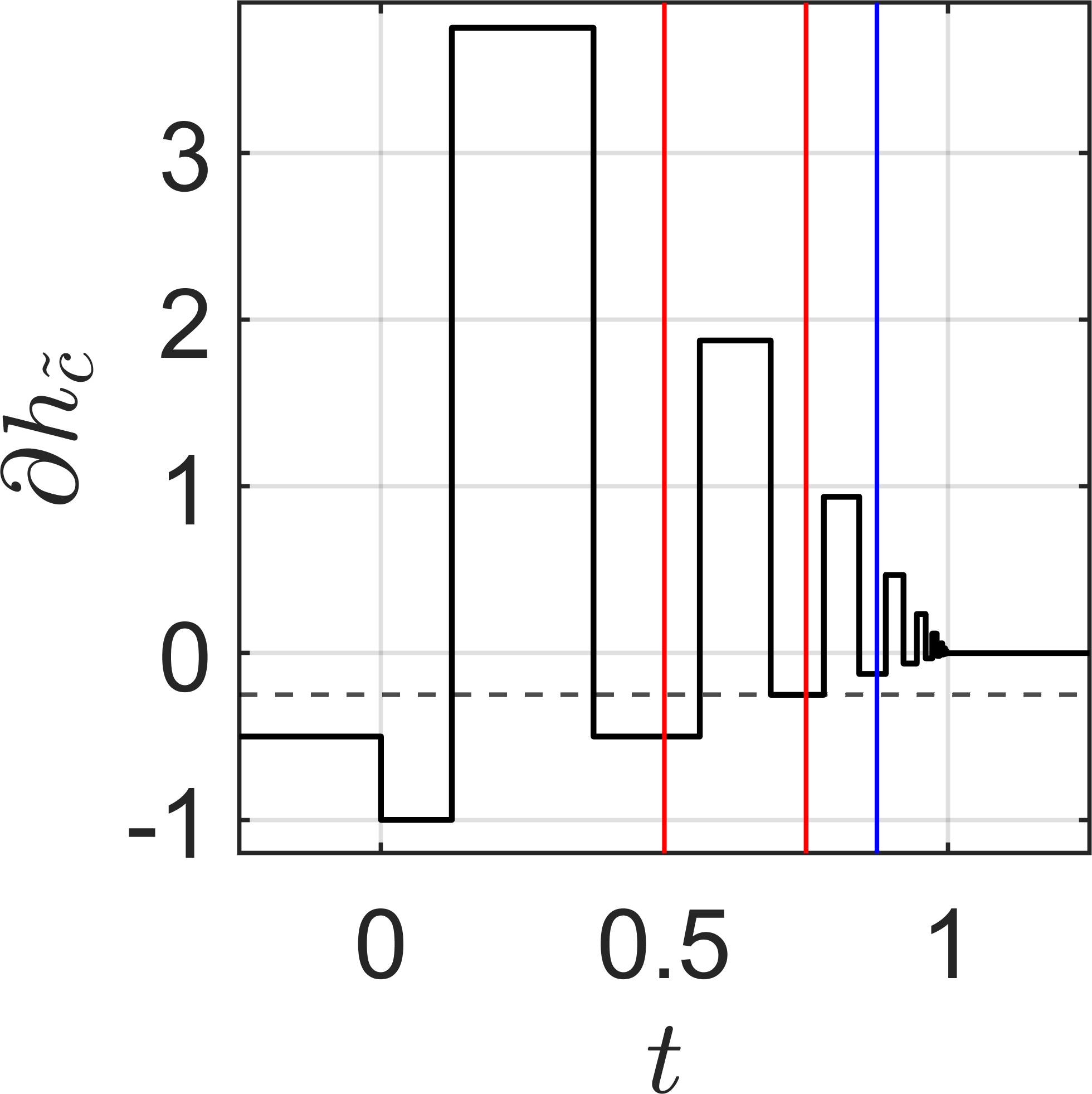
    Note that part (a) essentially solved the problem by simply choosing a different value for c𝑐c in hβ„Žh (leading to a more well-behaved function hc~subscriptβ„Ž~𝑐h_{\tilde{c}}). To better visualize differences of Algorithms 1 and 2, assume that we chose c=3/4𝑐34c=3/4, such that we may choose c~=1/2∈(cmin,c)~𝑐12subscript𝑐min𝑐\tilde{c}=1/2\in(c_{\text{min}},c). Then Algorithm 2 has to deal with the same problematic function as Algorithm 1 in Example 1. The resulting graphs of hc~subscriptβ„Ž~𝑐h_{\tilde{c}} and βˆ‚hc~subscriptβ„Ž~𝑐\partial h_{\tilde{c}} are shown in Figure 3.

    Refer to caption

    (a)

    Refer to caption

    (b)

    Figure 3: Same as Figure 2 but for c~=1/2~𝑐12\tilde{c}=1/2 and c=3/4𝑐34c=3/4.

    Since, in Algorithm 2, it is sufficient to have g>(c~βˆ’c)​‖v~β€–2𝑔~𝑐𝑐superscriptnorm~𝑣2g>(\tilde{c}-c)\|\tilde{v}\|^{2} for a subgradient g=βŸ¨ΞΎβ€²,v~⟩+c~​‖v~β€–2βˆˆβˆ‚hc~​(tj)𝑔superscriptπœ‰β€²~𝑣~𝑐superscriptnorm~𝑣2subscriptβ„Ž~𝑐subscript𝑑𝑗g=\langle\xi^{\prime},\tilde{v}\rangle+\tilde{c}\|\tilde{v}\|^{2}\in\partial h_{\tilde{c}}(t_{j}) (cf. (12)), and since all subgradients at hc~​(t)subscriptβ„Ž~𝑐𝑑h_{\tilde{c}}(t) tend to 00 as tβ†’1→𝑑1t\rightarrow 1, the method already stops in t3=7/8subscript𝑑378t_{3}=7/8 with the new Ξ΅πœ€\varepsilon-subgradient ΞΎβ€²=βˆ’5/8βˆ‰conv(W)={βˆ’1}superscriptπœ‰β€²58convπ‘Š1\xi^{\prime}=-5/8\notin\operatorname*{conv}(W)=\{-1\}.

5 Conclusion and future work

In this article, we showed how the gap in the convergence theory of the deterministic gradient sampling methods from [6, 7, 8] can be closed for weakly lower semismooth functions by a more careful handling of the sufficient decrease condition in the bisection.

For future work, it might be worth to analyze the behavior of Algorithm 2 in a more general setting. In [18], the convergence theory for the original gradient sampling method from [4] was generalized to directionally Lipschitzian functions, and already in [4], gradient sampling was successfully applied to even more general, non-Lipschitzian functions. Furthermore, the general strategy of approximating the Ξ΅πœ€\varepsilon-subdifferential in a deterministic fashion as in [15, 6, 7, 8] may lead to interesting new methods when combined with other methods that rely on random sampling, like [13, 14]. In the long run, we believe that this strategy may lead one step closer to a unified framework for both gradient sampling and bundle methods. For example, when comparing the standard gradient sampling method in [4] and the bundle method of [15], one could β€œhide” all the null steps in the bundle method in a subroutine and end up with a method that is similar to the gradient sampling method, just with a different way to approximate the Ξ΅πœ€\varepsilon-subdifferential.

\bmhead

Data Availability Data sharing not applicable to this article as no datasets were generated or analyzed during the current study.

Declarations

\bmhead

Conflict of Interest The author has no competing interests to declare that are relevant to the content of this article.

Appendix A A drawback of random sampling

Example A.7.

For n>1𝑛1n>1 let pr:ℝn→ℝnβˆ’1,x↦(x1,…,xnβˆ’1)⊀:prformulae-sequenceβ†’superscriptℝ𝑛superscriptℝ𝑛1maps-toπ‘₯superscriptsubscriptπ‘₯1…subscriptπ‘₯𝑛1top\operatorname*{pr}:\mathbb{R}^{n}\rightarrow\mathbb{R}^{n-1},x\mapsto(x_{1},\dots,x_{n-1})^{\top}, be the projection onto the first nβˆ’1𝑛1n-1 components. Let

f:ℝn→ℝ,x↦|xnβˆ’β€–pr(x)β€–|+12​xn.:𝑓formulae-sequenceβ†’superscriptℝ𝑛ℝmaps-toπ‘₯subscriptπ‘₯𝑛normprπ‘₯12subscriptπ‘₯𝑛\displaystyle f:\mathbb{R}^{n}\rightarrow\mathbb{R},\quad x\mapsto|x_{n}-\|\operatorname*{pr}(x)\||+\frac{1}{2}x_{n}.

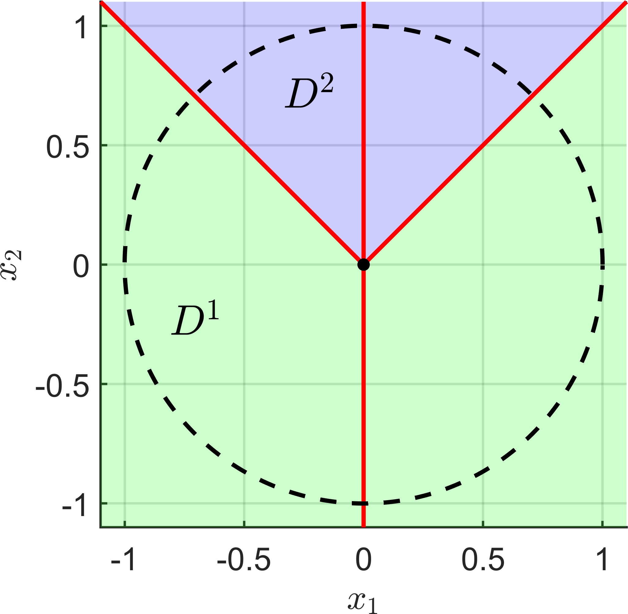
Then f𝑓f is continuously differentiable in D1βˆͺD2superscript𝐷1superscript𝐷2D^{1}\cup D^{2}, where

D1:={xβˆˆβ„n:pr(x)β‰ 0,xn<β€–pr(x)β€–},assignsuperscript𝐷1conditional-setπ‘₯superscriptℝ𝑛formulae-sequenceprπ‘₯0subscriptπ‘₯𝑛normprπ‘₯\displaystyle D^{1}:=\{x\in\mathbb{R}^{n}:\operatorname*{pr}(x)\neq 0,x_{n}<\|\operatorname*{pr}(x)\|\},
D2:={xβˆˆβ„n:pr(x)β‰ 0,xn>β€–pr(x)β€–}.assignsuperscript𝐷2conditional-setπ‘₯superscriptℝ𝑛formulae-sequenceprπ‘₯0subscriptπ‘₯𝑛normprπ‘₯\displaystyle D^{2}:=\{x\in\mathbb{R}^{n}:\operatorname*{pr}(x)\neq 0,x_{n}>\|\operatorname*{pr}(x)\|\}.

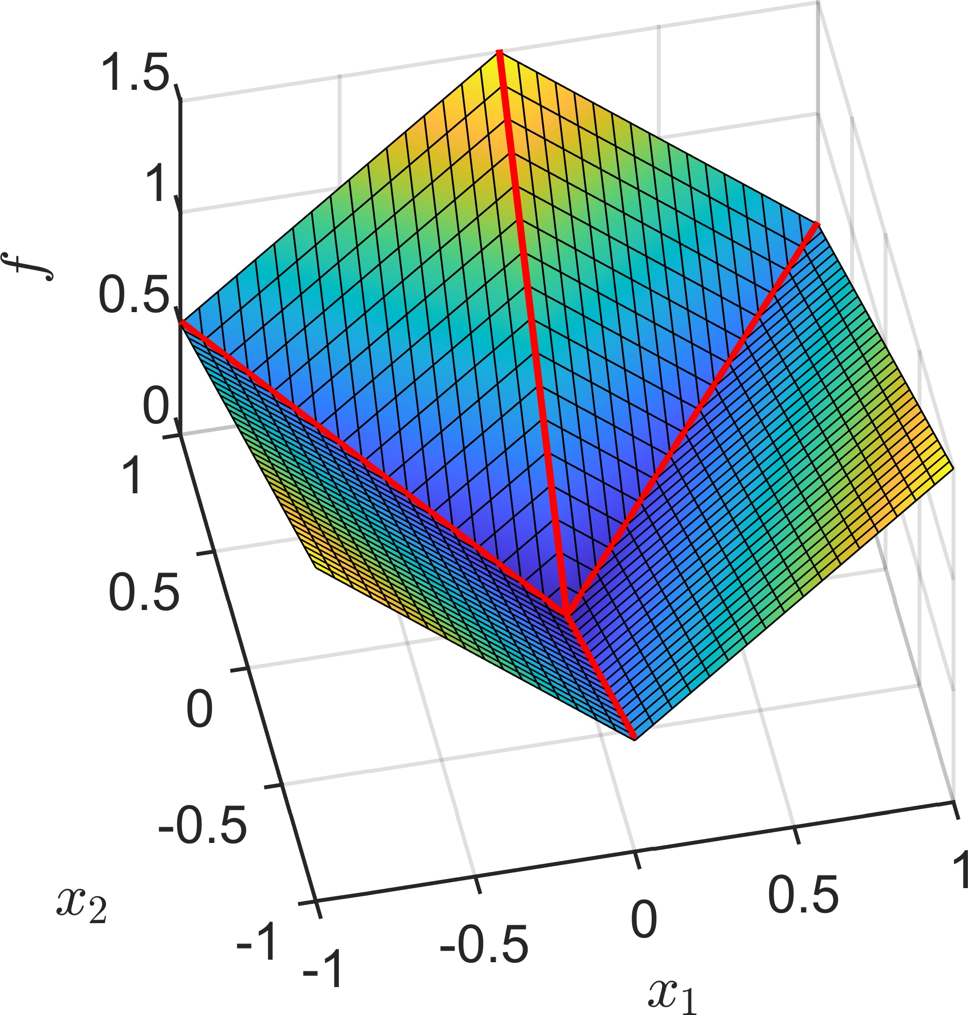
For n=2𝑛2n=2, the graph of f𝑓f and the sets D1superscript𝐷1D^{1}, D2superscript𝐷2D^{2} are shown in Figure 4.

Refer to caption

(a)

Refer to caption

(b)

Figure 4: (a) The graph of f𝑓f for n=2𝑛2n=2 in Example A.7. The red lines indicate the points in which f𝑓f is not differentiable. (b) The boundary of the unit sphere B1​(0)subscript𝐡10B_{1}(0) (dashed) and the sets D1superscript𝐷1D^{1} (green) and D2superscript𝐷2D^{2} (blue).

For the gradient we have

βˆ‡f​(x)=(pr(x)/β€–pr(x)β€–βˆ’1/2)β€‹βˆ€x∈D1,βˆ‡f​(x)=(βˆ’pr(x)/β€–pr(x)β€–3/2)β€‹βˆ€x∈D2.formulae-sequenceβˆ‡π‘“π‘₯matrixprπ‘₯normprπ‘₯12for-allπ‘₯superscript𝐷1βˆ‡π‘“π‘₯matrixprπ‘₯normprπ‘₯32for-allπ‘₯superscript𝐷2\displaystyle\nabla f(x)=\begin{pmatrix}\operatorname*{pr}(x)/\|\operatorname*{pr}(x)\|\\ -1/2\end{pmatrix}\ \forall x\in D^{1},\ \nabla f(x)=\begin{pmatrix}-\operatorname*{pr}(x)/\|\operatorname*{pr}(x)\|\\ 3/2\end{pmatrix}\ \forall x\in D^{2}.

Thus, it is easy to see that x=0π‘₯0x=0 is a critical point of f𝑓f. In particular, if x0βˆˆβ„nsubscriptπ‘₯0superscriptℝ𝑛x_{0}\in\mathbb{R}^{n} and Ξ΅>0πœ€0\varepsilon>0 such that 0∈BΡ​(x0)0subscriptπ΅πœ€subscriptπ‘₯00\in B_{\varepsilon}(x_{0}), then the solution of (3) is vΒ―=0¯𝑣0\bar{v}=0.
Clearly, to have vGS=0superscript𝑣GS0v^{\text{GS}}=0 in (6), it is necessary to sample at least one gradient from DΞ΅2:=D2∩BΡ​(x0)assignsuperscriptsubscriptπ·πœ€2superscript𝐷2subscriptπ΅πœ€subscriptπ‘₯0D_{\varepsilon}^{2}:=D^{2}\cap B_{\varepsilon}(x_{0}). For x0=0subscriptπ‘₯00x_{0}=0 and Ξ΅=1πœ€1\varepsilon=1, the probability that y∈DΞ΅2𝑦superscriptsubscriptπ·πœ€2y\in D_{\varepsilon}^{2} for a uniformly sampled y∈BΡ​(x0)𝑦subscriptπ΅πœ€subscriptπ‘₯0y\in B_{\varepsilon}(x_{0}) can be computed by comparing the hypervolume Vn​(DΞ΅2)subscript𝑉𝑛superscriptsubscriptπ·πœ€2V_{n}(D_{\varepsilon}^{2}) of DΞ΅2superscriptsubscriptπ·πœ€2D_{\varepsilon}^{2} (which can be computed via a partition of DΞ΅2superscriptsubscriptπ·πœ€2D_{\varepsilon}^{2} into a hypercone and a hyperspherical cap) to Vn​(BΡ​(x0))subscript𝑉𝑛subscriptπ΅πœ€subscriptπ‘₯0V_{n}(B_{\varepsilon}(x_{0})). In [4], m=2​nπ‘š2𝑛m=2n gradients are sampled in every iteration for the approximation of βˆ‚Ξ΅f​(x0)subscriptπœ€π‘“subscriptπ‘₯0\partial_{\varepsilon}f(x_{0}). The resulting probabilities of having at least one of the 2​n2𝑛2n sample points in DΞ΅2superscriptsubscriptπ·πœ€2D_{\varepsilon}^{2} are shown in Table 1.

Table 1: Probability that at least one of the 2​n2𝑛2n sample points lies in DΞ΅2superscriptsubscriptπ·πœ€2D_{\varepsilon}^{2} in Example A.7.
n𝑛n 222 333 555 101010 202020 505050 100100100
Prob. 0.68360.68360.6836 0.61330.61330.6133 0.45020.45020.4502 0.13940.13940.1394 0.00670.00670.0067 3.3β‹…10βˆ’7β‹…3.3superscript1073.3\cdot 10^{-7} 2.2β‹…10βˆ’14β‹…2.2superscript10142.2\cdot 10^{-14}

We see that when increasing the dimension n𝑛n, it quickly becomes highly unlikely that random gradient sampling correctly identifies x0=0subscriptπ‘₯00x_{0}=0 as Ξ΅πœ€\varepsilon-critical. Note that this is not related to x0=0subscriptπ‘₯00x_{0}=0 being a nonsmooth point of f𝑓f, and we get a similar (or even worse) result when choosing some x0∈D1subscriptπ‘₯0superscript𝐷1x_{0}\in D^{1} close to zero. (It would just become more difficult to compute the exact probabilities as in the table for x0β‰ 0subscriptπ‘₯00x_{0}\neq 0.) In this case, the method from [4] would perform descent steps with short step lengths (and little descent), which would require many function evaluations due to the backtracking nature of the line search, without recognizing that the iterates are already Ξ΅πœ€\varepsilon-critical.
If deterministic sampling is used instead (cf. Section 2.2), then a simple computation shows that if the first two subgradients ΞΎ1superscriptπœ‰1\xi^{1} and ΞΎ2superscriptπœ‰2\xi^{2} were sampled from D1superscript𝐷1D^{1}, then the next v~~𝑣\tilde{v} from (7) (for W={ΞΎ1,ΞΎ2}π‘Šsuperscriptπœ‰1superscriptπœ‰2W=\{\xi^{1},\xi^{2}\}) must be v~=(0,…,0,1/2)⊀~𝑣superscript0…012top\tilde{v}=(0,\dots,0,1/2)^{\top}, so the next subgradient is sampled at x0+1/2​v~subscriptπ‘₯012~𝑣x_{0}+1/2\ \tilde{v} (cf. Algorithm 2). If x0subscriptπ‘₯0x_{0} is close to zero, then x0+1/2​v~∈D2subscriptπ‘₯012~𝑣superscript𝐷2x_{0}+1/2\ \tilde{v}\in D^{2} such that a subgradient from D2superscript𝐷2D^{2} is sampled. After at most one additional iteration, the procedure stops and correctly obtains v~=vΒ―=0~𝑣¯𝑣0\tilde{v}=\bar{v}=0. Thus, for arbitrary n𝑛n, at most 444 subgradients have to be sampled when sampling deterministically.

References

  • \bibcommenthead
  • Clarke [1990] Clarke, F.H.: Optimization and Nonsmooth Analysis. Society for Industrial and Applied Mathematics, Philadelphia (1990). https://doi.org/10.1137/1.9781611971309
  • Goldstein [1977] Goldstein, A.A.: Optimization of lipschitz continuous functions. Mathematical Programming 13(1), 14–22 (1977) https://doi.org/10.1007/bf01584320
  • Burke etΒ al. [2002] Burke, J.V., Lewis, A.S., Overton, M.L.: Approximating Subdifferentials by Random Sampling of Gradients. Mathematics of Operations Research 27(3), 567–584 (2002) https://doi.org/10.1287/moor.27.3.567.317
  • Burke etΒ al. [2005] Burke, J.V., Lewis, A.S., Overton, M.L.: A Robust Gradient Sampling Algorithm for Nonsmooth, Nonconvex Optimization. SIAM Journal on Optimization 15(3), 751–779 (2005) https://doi.org/10.1137/030601296
  • Burke etΒ al. [2020] Burke, J.V., Curtis, F.E., Lewis, A.S., Overton, M.L., SimΓ΅es, L.E.A.: Gradient Sampling Methods for Nonsmooth Optimization. In: Numerical Nonsmooth Optimization: State of the Art Algorithms, pp. 201–225. Springer, Cham (2020). https://doi.org/10.1007/978-3-030-34910-3_6
  • Mahdavi-Amiri and Yousefpour [2012] Mahdavi-Amiri, N., Yousefpour, R.: An Effective Nonsmooth Optimization Algorithm for Locally Lipschitz Functions. Journal of Optimization Theory and Applications 155(1), 180–195 (2012) https://doi.org/10.1007/s10957-012-0024-7
  • Gebken and Peitz [2021] Gebken, B., Peitz, S.: An Efficient Descent Method for Locally Lipschitz Multiobjective Optimization Problems. Journal of Optimization Theory and Applications 80, 3–29 (2021) https://doi.org/10.1007/s10957-020-01803-w
  • Gebken [2022] Gebken, B.: Computation and analysis of Pareto critical sets in smooth and nonsmooth multiobjective optimization. PhD Thesis, Paderborn University (2022) https://doi.org/10.17619/UNIPB/1-1327
  • Mifflin [1977] Mifflin, R.: An algorithm for constrained optimization with semismooth functions. Mathematics of Operations Research 2(2), 191–207 (1977) https://doi.org/10.1287/moor.2.2.191
  • Lewis and Overton [2013] Lewis, A.S., Overton, M.L.: Nonsmooth optimization via quasi-Newton methods. Mathematical Programming 141, 135–163 (2013) https://doi.org/10.1007/s10107-012-0514-2
  • Mifflin [1977] Mifflin, R.: Semismooth and Semiconvex Functions in Constrained Optimization. SIAM Journal on Control and Optimization 15(6), 959–972 (1977) https://doi.org/10.1137/0315061
  • Sun and Sun [2008] Sun, D., Sun, J.: LΓΆwner’s Operator and Spectral Functions in Euclidean Jordan Algebras. Mathematics of Operations Research 33(2), 421–445 (2008) https://doi.org/10.1287/moor.1070.0300
  • Curtis and Que [2013] Curtis, F.E., Que, X.: An adaptive gradient sampling algorithm for non-smooth optimization. Optimization Methods and Software 28(6), 1302–1324 (2013) https://doi.org/10.1080/10556788.2012.714781
  • Curtis and Que [2015] Curtis, F.E., Que, X.: A quasi-Newton algorithm for nonconvex, nonsmooth optimization with global convergence guarantees. Mathematical Programming Computation 7(4), 399–428 (2015) https://doi.org/10.1007/s12532-015-0086-2
  • Kiwiel [2009] Kiwiel, K.C.: Improved Convergence Result for the Discrete Gradient and Secant Methods for Nonsmooth Optimization. Journal of Optimization Theory and Applications 144(1), 69–75 (2009) https://doi.org/10.1007/s10957-009-9584-6
  • LemarΓ©chal [1989] LemarΓ©chal, C.: Chapter VII. Nondifferentiable Optimization. In: Handbooks in Operations Research and Management Science, pp. 529–572. Elsevier, Amsterdam (1989). https://doi.org/10.1016/s0927-0507(89)01008-x
  • Cheney and Goldstein [1959] Cheney, W., Goldstein, A.A.: Proximity maps for convex sets. Proceedings of the American Mathematical Society 10(3), 448–448 (1959) https://doi.org/10.1090/s0002-9939-1959-0105008-8
  • Burke and Lin [2021] Burke, J.V., Lin, Q.: Convergence of the gradient sampling algorithm on directionally lipschitz functions. Set-Valued and Variational Analysis 29(4), 949–966 (2021) https://doi.org/%****␣main.bbl␣Line␣300␣****10.1007/s11228-021-00610-3