Numerical computation of quasinormal modes
in
the first-order approach to black hole perturbations in modified gravity

Abstract

We present a novel approach to the numerical computation of quasi-normal modes, based on the first-order (in radial derivative) formulation of the equations of motion and using a matrix version of the continued fraction method. This numerical method is particularly suited to the study of static black holes in modified gravity, where the traditional second-order, Schrödinger-like, form of the equations of motion is not always available. Our approach relies on the knowledge of the asymptotic behaviours of the perturbations near the black hole horizon and at spatial infinity, which can be obtained via the systematic algorithm that we have proposed recently. In this work, we first present our method for the perturbations of a Schwarzschild black hole and show that we recover the well-know frequencies of the QNMs to a very high precision. We then apply our method to the axial perturbations of an exact black hole solution in a particular scalar-tensor theory of gravity. We also cross-check the obtained QNM frequencies with other numerical methods.

I Introduction

The recent detection of gravitational waves (GW) has opened a new window on gravitational physics by giving unprecedented access to the regime of strong gravity. So far, the GW measurements are in good agreement with the predictions of general relativity (GR), but the rapidly increasing number of events and the improved sensitivity of the detectors expected in the near future will enable to verify GR to a high degree of precision or, alternatively, to detect some deviations from GR.

In this perspective, it is important to consider alternative theories of gravity, or extensions of GR, and study how their predictions deviate from GR, so that future analyses can extract the most relevant information from upcoming GW data. Most extensions of GR are scalar-tensor theories, which involve, directly or in disguise, a scalar field in addition to the usual metric tensor. The most general scalar-tensor theories that propagate a single scalar degree of freedom have been classified within the framework of DHOST theories, allowing for higher-order derivatives of the scalar field in the action Langlois:2015cwa ; Langlois:2015skt ; BenAchour:2016cay ; Crisostomi:2016czh ; BenAchour:2016fzp (see Langlois:2018dxi ; Kobayashi:2019hrl for reviews). These theories possess a very rich phenomenology and admit a number of exact static and spherically symmetric solutions (black holes or more exotic objects) even though very few exact rotating solutions are known Babichev:2017guv ; BenAchour:2018dap ; Motohashi:2019sen ; Charmousis:2019vnf ; Minamitsuji:2019shy ; BenAchour:2020wiw ; Minamitsuji:2019tet ; Anson:2020trg ; BenAchour:2020fgy ; Takahashi:2020hso ; Babichev:2020qpr ; Baake:2020tgk ; Capuano:2023yyh ; Bakopoulos:2023fmv (see also the review Babichev:2023psy ).

In the GW signal from a binary black hole merger, the ringdown phase is particularly interesting as it can be described by linear perturbations about a stationary black hole (BH) and is therefore easier to predict in theories of modified gravity than the whole inspiral phase. The ringdown signal mainly corresponds to a superposition of quasinormal modes, whose frequencies are quantised (see e.g. Kokkotas:1999bd ; Nollert:1999ji ; Berti:2009kk ; Konoplya:2011qq for reviews) and its detailed analysis via so-called “black hole spectroscopy”, represents an invaluable tool to test GR and look for characteristic signatures of modified gravity Berti:2005ys ; Berti:2018vdi .

In parallel to semi-analytical methods (see e.g. Hui:2022vov for recent works), many numerical techniques have been developed to compute QNMs Berti:2009kk ; Pani:2013pma ; Franchini:2023eda . One particularly efficient method was introduced by Leaver Leaver:1985ax , who managed to compute a large number of QNMs for the Schwarzschild and Kerr solutions with a high level of accuracy. His idea was to start from the equation of motion for the BH perturbations, written in the form of a second-order Schrödinger-like equation, thanks to the seminal works of Regge-Wheeler Regge:1957td and Zerilli Zerilli:1970se for Schwarzschild, and of Teukolsky Teukolsky:1973ha for Kerr, and to construct an ansatz for the solution that automatically implements the appropriate boundary conditions near the BH horizon and at spatial infinity. The ansatz depends on a bounded function, which can be expanded in a power series, and the equation of motion translates into a three-term recurrence relation for the coefficients of the series. A viable solution corresponds to a convergent series, associated with the so-called minimal solution of the recurrence relation, which can be obtained by solving a continued-fraction equation.

In theories of modified gravity, the equations of motion for the BH perturbations become more complicated than in GR and a nice second-order Schrödinger-like equation is not always available. This is why we have recently developed a new approach that directly extracts the asymptotic behaviour of the perturbations from the first-order system of the equations of motion Langlois:2021xzq . In the present work, we use this approach to construct an ansatz for the solution of the first-order system, with the appropriate asymptotic behaviour. The ansatz now depends on several bounded functions which, when expressed in power series, must satisfy a matrix recurrence relation, which we solve numerically by using a matricial version of the continued fraction method.

In order to test this new numerical technique we have first applied it to the familiar Schwarzschild case, starting directly from the first-order system of equations, in contrast with Leaver’s approach. We show that the well-known QNM frequencies for Schwarzschild can be recovered in this way, with a high precision. We then consider the axial perturbations of an exact BH solution in a scalar-tensor theory, constructed in Babichev:2017guv and dubbed BCL here, which can be seen as a one-parameter deformation of Schwarzschild. Using our first-order approach, we compute numerically the QNM frequencies of the axial perturbations, for different values of the parameter. We also cross-check the robustness of our technique with different numerical tests and comparison with other methods. While the first-order system we study is of dimension 2, our method can in principle be applied to higher-dimensional systems such as the ones appearing in the polar sector of perturbations Langlois:2021aji ; Langlois:2022eta . Note that a first order approach has already been used, in a case where the asymptotic analysis of the perturbations is straightforward, to compute numerically QNMs with a shooting method (e.g. in Blazquez-Salcedo:2016enn ; Blazquez-Salcedo:2017txk for Einstein-Gauss-Bonnet-Dilaton gravity).

This paper is structured as follows. In the next section, after a brief review of the derivation of the equations of motion in the Schwarzschild case, we explain in detail the method of matrix continued fraction for solving the first-order system of equations and show that we recover the standard values of the Schwarzschild QNMs. In the subsequent section, we present the exact BH in modified gravity and give the first-order system of equations satisfied by the axial perturbations. In section IV, we apply our numerical technique to this new system and obtain the QNMs, which depend on a single parameter, thus providing a continuum of modes in the complex plane relating the Schwarzschild BH QNMs and those of this family of solutions. In section IV, we present numerical convergence and consistency checks. We finally conclude with some perspectives. We also provide some details and comparisons with other numerical methods in the appendices.

II Schwarzschild BH QNM spectrum

In this section, we briefly recall how to derive the equations for linear perturbations about a Schwarzschild BH in GR, obtaining directly a system of two coupled first-order equations. Then, we use this “simple” example to illustrate how one can adapt the well-known continuous fraction method (originally used to compute the spectrum of Schrödinger-like operators) to such a first order matrix system.

II.1 Dynamics of linear perturbations

II.1.1 Perturbation equations in a first-order system

To derive the equations of motion for the linear perturbations, we substitute in the GR action,

$$S_{\mathrm{GR}}[g_{\mu\nu}]=\int\differential[4]{x}\sqrt{-g}\,R\,,$$ (1)

the perturbed metric

$$g_{\mu\nu}=\bar{g}_{\mu\nu}+h_{\mu\nu}\,,$$ (2)

where $\bar{g}_{\mu\nu}$ is the background solution and $h_{\mu\nu}$ the perturbation, and expand the action up to quadratic order in $h_{\mu\nu}$. The dynamics of the perturbations is governed by the quadratic action $S_{\mathrm{quad}}$, which reads, when the Ricci tensor vanishes (since we are in vacuum),

$$S_{\mathrm{quad}}[h_{\mu\nu}]=\int\differential[4]{x}\sqrt{-\bar{g}}\Big{[} \quad\frac{1}{2}(\bar{\nabla}_{\mu}h)(\bar{\nabla}^{\mu}h)-2(\bar{\nabla}_{\mu}\tensor{h}{{}^{\mu}_{\nu}})(\bar{\nabla}_{\rho}\tensor{h}{{}_{\nu}^{\rho}})-(\bar{\nabla}_{\mu}h)(\bar{\nabla}_{\nu}\tensor{h}{{}^{\mu}{}^{\nu}})$$

$$\qquad+3(\bar{\nabla}_{\nu}\tensor{h}{{}_{\mu}{}_{\rho}})(\bar{\nabla}^{\rho}\tensor{h}{{}^{\mu}{}^{\nu}})-\frac{1}{2}(\bar{\nabla}_{\rho}\tensor{h}{{}_{\mu}{}_{\nu}})(\bar{\nabla}^{\rho}\tensor{h}{{}^{\mu}{}^{\nu}})-2\tensor{\bar{R}}{{}_{\mu}{}_{\rho}{}_{\nu}{}_{\sigma}}\tensor{h}{{}^{\mu}{}^{\nu}}\tensor{h}{{}^{\rho}{}^{\sigma}}\Big{]}\,,$$ (3)

where $\bar{R}_{\mu\nu\rho\sigma}$ is the Riemann tensor of the background metric $\bar{g}_{\mu\nu}$ and $\bar{\nabla}$ denotes the covariant derivative compatible with $\bar{g}_{\mu\nu}$.

For a static and spherically symmetric background, the metric is of the form

$$\bar{g}_{\mu\nu}\differential{x^{\mu}}\differential{x^{\nu}}=-A(r)\differential{t}^{2}+\frac{\differential{r}^{2}}{B(r)}+C(r)\differential{\Omega}^{2}\,,\\$$

and in the particular case of the Schwarzschild solution, we have

$$A(r)=B(r)=1-\frac{\mu}{r}\,,\quad C(r)=r^{2}\,,$$ (4)

where $\mu$ is a constant corresponding to twice the black hole mass.

The perturbations $h_{\mu\nu}$ are conveniently described via a $2+2$ decomposition onto the sphere, in which the various components are expanded in spherical harmonics $Y_{\ell m}(\theta,\varphi)$ according to

$$h_{tt} =A(r)\sum_{\ell,\,m}H_{0}^{\ell m}(t,r)Y_{\ell m}(\theta,\varphi)\,,$$

$$h_{tr} =\sum_{\ell,\,m}H_{1}^{\ell m}(t,r)Y_{\ell m}(\theta,\varphi)\,,$$

$$h_{rr} =\frac{1}{B(r)}\sum_{\ell,\,m}H_{2}^{\ell m}(t,r)Y_{\ell m}(\theta,\varphi)\,,$$

$$h_{ta} =\sum_{\ell,\,m}\quantity[\beta^{\ell}(t,r)\partial_{a}+h_{0}^{\ell m}(t,r)\sin\theta\,\epsilon_{ab}\partial^{b}]Y_{\ell m}(\theta,\varphi)\,,$$

$$h_{ra} =\sum_{\ell,\,m}\quantity[\alpha^{\ell m}(t,r)\partial_{a}+h_{1}^{\ell m}(t,r)\sin\theta\,\epsilon_{ab}\partial^{b}]Y_{\ell m}(\theta,\varphi)\,,$$

$$h_{ab}=\frac{1}{2}\sum_{\ell,\,m}h_{2}^{\ell m}(t,r)\sin\theta(\epsilon_{ac}\nabla^{c}\nabla_{b}+\epsilon_{bc}\nabla^{c}\nabla_{a})Y_{\ell m}(\theta,\varphi)\,$$

$$+\sum_{\ell,\,m}\quantity[K^{\ell m}(t,r)g_{ab}+G^{\ell m}(t,r)\nabla_{a}\nabla_{b}]Y_{\ell m}(\theta,\varphi)\,,$$ (5)

where $h_{0}$, $h_{1}$, $h_{2}$, $H_{0}$, $H_{1}$, $H_{2}$, $\alpha$, $\beta$, $K$ and $G$ are functions of $(t,r)$. The indices $a$ and $b$ denote the angular coordinates $\{\theta,\varphi\}$ and $\epsilon_{ab}$ is the fully antisymmetric tensor associated with the metric of the 2-sphere. Since there is no mixing between modes with different values of $\ell$ and $m$ at the linear level, we will drop these labels in the following. Furthermore, it is convenient to work in the frequency domain so that any function $f(t,r)$ is replaced by ${f}(r)e^{-i\omega t}$.

The equations of motion for the perturbations are given by

$$\mathcal{E}_{\mu\nu}\vcentcolon=\functionalderivative{S_{\mathrm{quad}}}{h_{\mu\nu}}=0\,.$$ (6)

By a gauge transformation, one can always take $\alpha$, $\beta$, $G$ and $h_{2}$ to be zero Kobayashi:2012kh ; Kobayashi:2014wsa : this is the well-known Regge-Wheeler gauge Regge:1957td . Substituting the expressions (5) into the perturbation equations (6) yields two decoupled systems (see Langlois:2021xzq ) which can be written in a matrix form as follows,

$$\derivative{X_{\mathrm{ax}}}{r}=M_{\mathrm{ax}}X_{\mathrm{ax}}\,,\qquad\derivative{X_{\mathrm{po}}}{r}=M_{\mathrm{pol}}X_{\mathrm{pol}}\,.$$ (7)

The first system corresponds to axial perturbations of the Schwarzschild black hole with

$$X_{\mathrm{ax}}=\begin{pmatrix}h_{0}\\ h_{1}\end{pmatrix}\mbox{\quad and\quad}M_{\mathrm{ax}}=\begin{pmatrix}\frac{2}{r}&-i\omega+\frac{2i\lambda(r-\mu)}{\omega r^{3}}\\ -\frac{i\omega r^{2}}{(r-\mu)^{2}}&-\frac{\mu}{r(r-\mu)}\end{pmatrix}\,,$$ (8)

where

$$\lambda=\frac{\ell(\ell+1)}{2}-1\,.$$ (9)

The second system corresponds to polar perturbations with

$$X_{\mathrm{pol}}=\begin{pmatrix}K\\ \ifrac{H_{1}}{\omega}\end{pmatrix}\quad\text{and}$$

$$M_{\mathrm{pol}}=\frac{1}{3\mu+2\lambda r}\begin{pmatrix}\frac{\mu(3\mu+(\lambda-2)r)-2r^{4}\omega^{2}}{r(r-\mu)}&\frac{2i(\lambda+1)(\mu+\lambda r)+2ir^{3}\omega^{2}}{r^{2}}\\ \frac{ir\left(9\mu^{2}-8\lambda r^{2}+8(\lambda-1)\mu r\right)+4ir^{5}\omega^{2}}{2(r-\mu)^{2}}&\frac{2r^{4}\omega^{2}-\mu(3\mu+3\lambda r+r)}{r(r-\mu)}\\ \end{pmatrix}\,.$$ (10)

In the following, we focus our attention on the system of axial perturbations.

II.1.2 Definition of quasinormal modes

As described in Langlois:2021xzq , one can extract the asymptotic behaviours of the perturbations, at the horizon and at spatial infinity, directly from the first-order system (8) by resorting to an asymptotic expansion of the matrix $M_{\mathrm{ax}}$.

Introducing the traditional tortoise coordinate defined by

$$\derivative{r_{*}}{r}=\frac{1}{1-\ifrac{\mu}{r}}\,\Longrightarrow\;r_{*}=r+\mu\ln(r-\mu)\,,$$ (11)

the leading-order terms in the asymptotic expansion of the perturbations at the horizon (i.e. when $r\to\mu$ or equivalently $r_{*}\to-\infty$) were found to be given by Langlois:2021xzq

$$h_{0}(r) =(c^{\mathrm{hor}}_{+}e^{i\omega r_{*}}+c^{\mathrm{hor}}_{-}e^{-i\omega r_{*}})(1+\mathcal{O}(r-\mu))\,,$$

$$h_{1}(r) =\frac{\mu}{r-\mu}(-c^{\mathrm{hor}}_{+}e^{i\omega r_{*}}+c^{\mathrm{hor}}_{-}e^{-i\omega r_{*}})(1+\mathcal{O}(r-\mu))\,,$$ (12)

where $c^{\mathrm{hor}}_{\pm}$ are constants. At spatial infinity, i.e. when $r,r_{*}\to+\infty$ , the corresponding leading-order expressions are Langlois:2021xzq

$$h_{0}(r) =r(c^{\infty}_{-}e^{-i\omega r_{*}}-c^{\infty}_{+}e^{i\omega r_{*}})(1+\mathcal{O}(1/r))\,,$$

$$h_{1}(r) =r(c^{\infty}_{-}e^{-i\omega r_{*}}+c^{\infty}_{+}e^{i\omega r_{*}})(1+\mathcal{O}(1/r))\,,$$ (13)

where $c^{\infty}_{\pm}$ are other constants and $r_{*}=r(1+{o}(r))$ at infinity.

Moreover, restoring the time dependence in $e^{-i\omega t}$, one sees that the asymptotic terms in (12) and (13), consist of the superposition of an ingoing mode, proportional to $e^{-i\omega(t+r_{*})}$, and of an outgoing mode, proportional to $e^{-i\omega(t-r_{*})}$, propagating radially along the coordinate $r_{*}$ at speed 1.

Quasinormal modes are the perturbations that are purely ingoing at the BH horizon and outgoing at spatial infinity, which is possible only for a discrete set of specific frequencies. Therefore, identifying the QNMs means finding the complex values $\omega$ such that the solution to (8) satisfies

$$c^{\infty}_{-}=0\mbox{\quad and\quad}c^{\mathrm{hor}}_{+}=0\,.$$ (14)

We will see in the following subsection, how these QNM frequencies can be determined numerically.

II.2 Matrix continued fraction

We show below how to adapt the continuous fraction method to compute QNMs directly from the first order system, without using a Schrödinger-like reformation of the perturbations equations, as in the seminal work by Leaver Leaver:1985ax .

II.2.1 Boundary conditions and ansatz

Imposing the QNM boundary conditions (14) in the general asymptotic behaviours of $X_{\mathrm{ax}}$ and using $e^{i\omega r_{*}}=e^{i\omega r}(r-\mu)^{i\mu\omega}$, which follows from (11), we get

$$X_{\mathrm{ax}}(r) = c_{-}^{\mathrm{hor}}\,e^{-i\omega r}(r-\mu)^{-i\mu\omega}\begin{pmatrix}r-\mu\\ \mu\end{pmatrix}\left(\frac{1}{r-\mu}+\mathcal{O}(1)\right)\,,\quad\text{when}\quad r\to\mu\,,$$ (15)

$$X_{\mathrm{ax}}(r) = c_{+}^{\infty}\,e^{i\omega r}(r-\mu)^{i\mu\omega}\begin{pmatrix}-1\\ 1\end{pmatrix}(r+{\cal O}(1))\,,\quad\text{when}\quad r\to+\infty\,.$$ (16)

In order to find a solution that satisfies simultaneously these two behaviours at the boundaries, one starts with an ansatz of the form

$$X_{\mathrm{ax}}(r)=e^{i\omega r}r^{1+i\mu\omega}\quantity(\frac{r-\mu}{r})^{-i\mu\omega}\times\begin{pmatrix}f_{0}(u)\\ f_{1}(u)/u\end{pmatrix}\mbox{\quad with\quad}u=\frac{r-\mu}{r}\,.$$ (17)

The two complex-valued functions $f_{0}$ and $f_{1}$ are supposed to be bounded (with no singularities) for $u\in[0,1]$ and should satisfy the boundary conditions

$$f_{0}(0)=f_{1}(0)\,,\qquad f_{0}(1)=-f_{1}(1)\,,$$ (18)

so that the appropriate asymptotic behaviours are indeed obtained.

II.2.2 Recurrence relation

As the two functions are bounded for $u\in[0,1]$, they can be expanded in power series as follows,

$$f_{0}(u)=\sum_{n=0}^{\infty}a_{n}u^{n}\mbox{\quad and\quad}f_{1}(u)=\sum_{n=0}^{\infty}b_{n}u^{n}\,,$$ (19)

where $a_{n}$ and $b_{n}$ are complex numbers. Substituting the ansatz  (17) together with the expressions (19) into the equations of motion  (8) leads to a recurrence relation for the coefficients $a_{n}$ and $b_{n}$. In order to write this recurrence relation in a compact form, it is convenient to view the coefficients $a_{n}$ and $b_{n}$ as the components of 2-dimensional vectors $Y_{n}$, i.e.

$$Y_{n}=\begin{pmatrix}a_{n}\\ b_{n}\end{pmatrix}\,,$$ (20)

which in turn satisfy the relations

$$\alpha_{n}Y_{n+1}+\beta_{n}Y_{n}+\gamma_{n}Y_{n-1}+\delta_{n}Y_{n-2}=0\,,\qquad\forall n\geq 2\,,$$ (21)

where the matrix coefficients are given by

$$\alpha_{n} =\begin{pmatrix}\frac{n+1-i\mu\omega}{\mu}&i\omega\\ i\mu^{2}\omega&\mu(n+1-i\mu\omega)\end{pmatrix}\,, \beta_{n}= \begin{pmatrix}\frac{-2n-1+4i\mu\omega}{\mu}&\ifrac{-2i\lambda}{\mu^{2}\omega}\\ 0&\mu(-2n+1+4i\mu\omega)\end{pmatrix}\,,$$

$$\gamma_{n} =\begin{pmatrix}\frac{n}{\mu}-2i\omega&\ifrac{4i\lambda}{\mu^{2}\omega}\\ 0&\mu(n-2-2i\mu\omega)\end{pmatrix}\,, \delta_{n}= \begin{pmatrix}0&\ifrac{-2i\lambda}{\mu^{2}\omega}\\ 0&0\end{pmatrix}\,.$$ (22)

This relation (21) still holds for $0\leq n<2$ in which cases the number of terms is reduced, defining $\alpha_{n}=\beta_{n}=\gamma_{n}=\delta_{n}=0$ when $n<0$ by convention. When $n=0$, it reduces to a 2-term relation as it involves $Y_{1}$ and $Y_{0}$ only; when $n=1$, it is a 3-term relation between $Y_{2}$, $Y_{1}$ and $Y_{0}$.

In order to solve this 4-term recurrence relation (21), we first show that it can always be reformulated as a 3-term recurrence relation. To prove this is indeed possible, we proceed by induction. Hence, let us assume that it is possible to write (21) at some order $n$ in the form

$$\tilde{\alpha}_{n}Y_{n+1}+\tilde{\beta}_{n}Y_{n}+\tilde{\gamma}_{n}Y_{n-1}=0\,,$$ (23)

where $\tilde{\alpha}_{n}$, $\tilde{\beta}_{n}$ and $\tilde{\gamma}_{n}$ are matrices to be determined, a priori different from (22). If we assume, in addition, that the matrix $\tilde{\gamma}_{n}$ is invertible, then we can express $Y_{n-1}$ as an explicit linear combination of $Y_{n}$ and $Y_{n+1}$. As a consequence, the original 4-terms recurrence relation (21) at order $n+1$ can also be reformulated as a 3-term recurrence relation as follows,

$$\alpha_{n+1}Y_{n+2}+\quantity(\beta_{n+1}-\delta_{n+1}\cdot\tilde{\gamma}_{n}^{-1}\cdot\tilde{\alpha}_{n})Y_{n+1}+\quantity(\gamma_{n+1}-\delta_{n+1}\cdot\tilde{\gamma}_{n}^{-1}\cdot\tilde{\beta}_{n})Y_{n}=0\,.$$ (24)

As (21) reduces to a 3-terms relation for $n=1$ (and also a 2-terms relation for $n=0$), it is indeed possible to transform the recurrence relation into (23) for any $n$. The matrices entering in the 3-term recurrence relation are recursively defined by

$$\tilde{\alpha}_{n}=\alpha_{n}\,,\quad\tilde{\beta}_{n}=\beta_{n}-\delta_{n}\cdot\tilde{\gamma}_{n-1}^{-1}\cdot\tilde{\alpha}_{n-1}\,,\quad\tilde{\gamma}_{n}=\gamma_{n}-\delta_{n}\cdot\tilde{\gamma}_{n-1}^{-1}\cdot\tilde{\beta}_{n-1}\,,\quad\text{for}\quad n\geq 1\,,$$ (25)

with, at order $n=0$, the initial matrices

$$\tilde{\alpha}_{0}=\alpha_{0}\,,\qquad\tilde{\beta}_{0}=\beta_{0}\,,\qquad\tilde{\gamma}_{0}=0\,.$$ (26)

II.2.3 Convergence of the series

In general, three-term recurrence relations like (23) have solutions that can be expressed as a linear combination of two independent sequences (similarly to second order differential equations). However, not every solution will lead to the convergence of the power series (19) whereas the convergence of both power series is required in order to impose the right boundary condition at infinity. In the case of scalar recurrence relations (where $Y_{n}$ are complex numbers), a condition to ensure the convergence was found by Gautschi in gautschiComputationalAspectsThreeTerm1967 , in the form of an equation containing a continued fraction. It was then used by Leaver Leaver:1985ax to compute QNMs, leading to the “continued fraction method”.

Later, this study was generalised to recurrence relations where $Y_{n}$ are vectors linked by matrix-valued coefficients (see simmendingerAnalyticalApproachFloquet1999 ; Rosa:2011my ; Pani:2013pma for instance). Here, we apply these results to our problem to ensure that $f_{0}$ and $f_{1}$ are regular functions of $u$ in the whole interval $[0,1]$ with finite limits at the boundaries $u=0$ and $u=1$. This corresponds to choosing the appropriate branch for $Y_{n}$.

Let us proceed by first introducing invertible matrices $R_{n}$ such that

$$Y_{n+1}=R_{n}Y_{n}\,,\qquad\,n\geq 0\,.$$ (27)

Note that such relations do not uniquely define the matrices $R_{n}$. If one substitutes the above relation into the recurrence relation (23), one obtains

$$(\tilde{\alpha}_{0}R_{0}+\tilde{\beta}_{0})Y_{0}=0\,,\qquad(\tilde{\alpha}_{n}R_{n}+\tilde{\beta}_{n}+\tilde{\gamma}_{n}R_{n-1}^{-1})\,Y_{n}\;=\;0\qquad\text{for}\;\;n\geq 1\,.$$ (28)

This identity is trivially satisfied if the matrices $R_{n}$ themselves satisfy a recurrence relation which can be expressed as follows,

$$R_{n-1}=-(\tilde{\beta}_{n}+\tilde{\alpha}_{n}R_{n})^{-1}\tilde{\gamma}_{n}\,\qquad\text{for}\;\;n\geq 1\,.$$ (29)

Interestingly, when the matrices $R_{n}$ satisfy this relation, the power series defining the two functions $f_{0}$ and $f_{1}$ can be expected to be convergent. In other words, (29) selects the right branch for the solution $Y_{n}$. Furthermore, the zeroth order equation in (28) can be seen as a system of algebraic equations for $\omega$ whose solutions are the quasi-normal frequencies of the Schwarzschild black hole.

Remarkably, one can construct an infinite number of algebraic equations satisfied by the QNMs. Indeed, if we combine the $n=0$ order equation in (28) with (29) for $n=1$, we obtain a new equation which links $R_{1}$ to $Y_{1}$,

$$(\tilde{\alpha}_{0}R_{0}+\tilde{\beta}_{0})Y_{0}=(\tilde{\alpha}_{0}R_{0}+\tilde{\beta}_{0})R_{0}^{-1}R_{0}Y_{0}=\quantity[\tilde{\alpha}_{0}-\tilde{\beta}_{0}\tilde{\gamma}_{1}^{-1}(\tilde{\beta}_{1}+\tilde{\alpha}_{1}R_{1})]Y_{1}=0$$

$$\qquad\qquad\Longrightarrow\quantity[\tilde{\alpha}_{1}R_{1}+\tilde{\beta}_{1}-\tilde{\gamma}_{1}\tilde{\beta}_{0}^{-1}\tilde{\alpha}_{0}]Y_{1}=0\,.$$ (30)

It can be viewed again as an algebraic equation for the QNMs. Of course, we can proceed in this way recursively to obtain, at any order $n\geq 0$, relations of the form

$$(\tilde{\alpha}_{n}R_{n}+Q_{n})Y_{n}=0\,,$$ (31)

where the matrices $Q_{n}$ must satisfy

$$\text{for}\,n\geq 1,\quad Q_{n}=\tilde{\beta}_{n}-\tilde{\gamma}_{n}\cdot Q_{n-1}^{-1}\cdot\tilde{\alpha}_{n-1}\qquad\text{and}\quad Q_{0}=\tilde{\beta}_{0}\,.$$ (32)

Hence, the method is reminiscent of the usual construction of a continued fraction based on the Schrödinger-like formulation. At each order, the equation (31) can be seen as an algebraic equation for $\omega$ and then, each solution of this equation corresponds to a QNM. Of course, there exists a non-trivial solution of eq. (31) only when

$$\det(\tilde{\alpha}_{n}R_{n}+Q_{n})=0\,,$$ (33)

which is the equation we will solve numerically in the following section. In principle, (33) is necessary but not sufficient to satisfy (31). Therefore, we will need to check that the values of $\omega$ we obtain by solving the former equation also solve the latter. Further details on the numerical resolution will be given in the next subsection II.3.

II.3 Numerical method and results

The numerical method consists in applying a root-finding algorithm in the complex plane to determine the values of $\omega$ that solve (33), for given values of the black hole mass $2\mu$, of the angular momentum integer $\ell$, or equivalently $\lambda$, and the so-called inversion index $n$.

One must first determine the matrix $R_{n}$, which can be computed from $R_{n+1}$ via the inverse recurrence relation (29). In practice, in order to compute $R_{n}$ in a finite number of steps, a truncation is necessary at some large value $N$, where we impose the simple condition

$$R_{N}=0\,.$$ (34)

The precision on the quasi-normal frequency is then controlled by the value of the truncation index $N$. One should note that the value we choose for $R_{N}$ is arbitrary: it will introduce a small error which turns out to be negligible when $N$ is chosen to be large enough.

The other matrix appearing in (33), $Q_{n}$, is computed via the recurrence relation (32). The last step consists in finding the frequencies solving (33) thanks to the root-finding algorithm. One finally checks that the values thus obtained are stable when the truncation integer $N$ is increased.

We find empirically that increasing $n$ leads to a better precision for the computation of high-overtone modes. By choosing increasingly large values for $N$, we are able to compute several hundreds of QNMs for the Schwarzschild black hole, up to very high precision (around 10 digits). More details on the convergence and consistency checks are given in section V in the case of the BCL black hole. Since the Schwarzschild QNMs are well-known, we simply provide the first 20 frequencies obtained by our method in table 1. These values agree with existing data (for example Berti:2009kk ) up to the 6-digit precision we set for our computation, which confirms the validity of our method.

$\bm{n}$	$\bm{\omega_{n}}$
0	0.747343-0.177924i
1	0.693422-0.547830i
2	0.602107-0.956554i
3	0.503010-1.410296i
4	0.415029-1.893690i
5	0.338598-2.391216i
6	0.266504-2.895821i
7	0.185645-3.407682i
8	0.000000-3.999000i
9	0.126527-4.605289i

$\bm{n}$	$\bm{\omega_{n}}$
10	0.153107-5.121653i
11	0.165196-5.630884i
12	0.171456-6.137389i
13	0.174788-6.642460i
14	0.176478-7.146641i
15	0.177181-7.650211i
16	0.177265-8.153329i
17	0.176953-8.656100i
18	0.176381-9.158594i
19	0.175641-9.660860i

Table 1: Values computed for the QNMs of the Schwarzschild black hole using the first order system and the matrix continued fraction method. We set $\mu=1$ and $\lambda=2$ (corresponding to $\ell=2$). We focus only on modes with $\real(\omega)>0$; for each mode in this half-plane, there exists a mode with the same imaginary part and an opposite real part.

III BCL black hole in Scalar-Tensor Theories

We now consider an exact black hole solution in a scalar-tensor theory of gravity, for which we compute for the first time the axial quasi-normal modes, as presented in the next section.

III.1 BH solution in modified gravity

The scalar-tensor theory discussed here is described by an action of the form

$$S[g_{\mu\nu},\phi]=\int\differential^{4}{x}\sqrt{-g}\Big{[}F(X)R+P(X)+2\partialderivative{F}{X}(\phi_{\mu\nu}\phi^{\mu\nu}-(\square\phi)^{2})\Big{]}\,,$$ (35)

where $X\equiv\nabla^{\mu}\phi\nabla_{\mu}\phi$, $\phi_{\mu\nu}\equiv\nabla_{\mu}\nabla_{\nu}\phi$ and

$$F(X)=F_{0}+F_{1}\sqrt{X}\,,\qquad P(X)=-P_{1}X\,.$$ (36)

This action, which depends on second derivatives of the scalar field $\phi$, belongs to the subfamily of Horndeski theories Horndeski:1974wa , itself included in the general family DHOST theories discussed in the introduction.

Our motivation for choosing this specific theory is the existence of an exact BH solution, dubbed BCL solution after its authors Babichev:2017guv . It is described by the metric

$$\differential{s}^{2}=-A(r)\differential{t}^{2}+\frac{1}{B(r)}\differential{r}^{2}+C(r)\differential{\Omega}^{2}\,,$$ (37)

with

$$A(r)=B(r)=\quantity(1-\frac{r_{+}}{r})\quantity(1+\frac{r_{-}}{r})\,,\qquad C(r)=r^{2}\,,$$ (38)

where the (positive) quantities $r_{+}$ and $r_{-}$ are defined by

$$r_{+}r_{-}=\frac{F_{1}^{2}}{2F_{0}P_{1}}\,,\quad r_{+}-r_{-}=\mu\mbox{\quad and\quad}r_{+}>r_{-}>0\,.$$ (39)

The metric possesses only one horizon located at $r=r_{+}$ and the function $A$ can be rewritten as

$$A(r)=1-\frac{\mu}{r}-\frac{\mu^{2}\xi}{2r^{2}}\mbox{\quad with\quad}\xi=\frac{2r_{+}r_{-}}{\mu^{2}}\,,$$ (40)

which shows that $\mu$ corresponds to twice the ADM mass, as previously in the Schwarzschild case.

As for the scalar field, its configuration is given by

$$\phi(r)=\pm\frac{f_{1}}{{p_{1}}\sqrt{r_{+}r_{-}}}\arctan\left[\frac{(r_{+}-r_{-})r+2r_{+}r_{-}}{2\sqrt{r_{+}r_{-}}\sqrt{(r-r_{+})(r+r_{-})}}\right]\,+{\text{cst}}\,.$$ (41)

The global sign of $\phi(r)$ and the constant are physically irrelevant Babichev:2017guv .

Interestingly, the above solution can be seen as a one-parameter deformation of the Schwarzschild solution, with $r_{-}$ playing the role of the deformation parameter. In the limit $r_{-}=0$, corresponding to $F_{1}=0$, one recovers precisely the Schwarzschild metric, while the scalar field vanishes.

III.2 Perturbation equations

To obtain the equations of motion for the linear perturbations, one proceeds similarly to the GR case presented in section II.1. We substitute in the action (35) the metric and scalar field

$$g_{\mu\nu} =\bar{g}_{\mu\nu}+h_{\mu\nu}\,,\qquad\phi=\bar{\phi}+\variation{\phi}\,,$$ (42)

where $\bar{g}_{\mu\nu}$ and $\bar{\phi}$ are respectively the metric and scalar field of the background, while $h_{\mu\nu}$ and $\variation{\phi}$ are the corresponding perturbations.

We then expand the action (35) up to quadratic order in $h_{\mu\nu}$ and $\delta\phi$, and obtain (after some calculations) the quadratic action for linear perturbations

$$S_{\mathrm{quad}}[h_{\mu\nu},\variation{\phi}]\,.$$ (43)

The equations of motion for the perturbations are then given by the Euler-Lagrange equations,

$$\mathcal{E}_{\mu\nu}=\frac{\delta S_{\mathrm{quad}}}{\delta h_{\mu\nu}}=0\mbox{\quad and\quad}\mathcal{E}_{\phi}=\frac{\delta S_{\mathrm{quad}}}{\delta(\variation{\phi})}=0\,.$$ (44)

One can check that the equation $\mathcal{E}_{\phi}=0$ is redundant due to Bianchi’s identities.

In the following, we only consider axial perturbations, for which the perturbation of the scalar field vanishes, i.e. $\variation{\phi}=0$. The situation is then analogous to the GR case, although the equations of motion are now different. As shown in Langlois:2021aji , we obtain the first-order system

$$\derivative{X_{\mathrm{ax}}}{r}=M_{\mathrm{ax}}X_{\mathrm{ax}}$$ (45)

with

$$X_{\mathrm{ax}}=\begin{pmatrix}h_{0}\\ h_{1}\end{pmatrix}\,,\qquad\qquad M_{\mathrm{ax}}=\begin{pmatrix}\frac{2}{r}&-i\omega+\frac{2i\lambda(r-r_{+})(r+r_{-})}{r^{4}\omega}\\ -\frac{i\omega r^{2}(r^{2}+2r_{-}r_{+})}{(r-r_{+})^{2}(r-r_{-})^{2}}&-\frac{r(r_{+}-r_{-})+2r_{+}r_{-}}{r(r-r_{+})(r+r_{-})}\,\end{pmatrix}\,.$$ (46)

As we can see, we recover the Schwarzschild system (8) in the limit $r_{-}=0$, where $\mu=r_{+}$.

IV Axial quasinormal modes of the BCL Black Hole

In this section, we compute the axial QNMs of the BCL black hole using the “matrix continued fraction” method introduced earlier for Schwarzschild. Then, we compare our results with those obtained from already existing methods to perform consistency checks.

IV.1 Ansatz and recurrence relation

In order to guess an appropriate ansatz, we need the asymptotic behaviours of axial perturbations at both the horizon and spatial infinity. They have already been computed in Langlois:2021aji where we found that the leading-order terms in the asymptotic expansion at spatial infinity (when $r\to\infty$) are given by

$$h_{0}(r) =r(c^{\infty}_{+}e^{i\omega r}r^{i\mu\omega}-c^{\infty}_{-}e^{-i\omega r}r^{-i\mu\omega})(1+\mathcal{O}(1/r))\,,$$

$$h_{1}(r) =r(c^{\infty}_{+}e^{i\omega r}r^{i\mu\omega}+c^{\infty}_{-}e^{-i\omega r}r^{-i\mu\omega})(1+\mathcal{O}(1/r))\,,$$ (47)

where $c^{\infty}_{\pm}$ are constant. And the asymptotic expansion near the horizon (when $r\to r_{+}$) yields, at leading order,

$$h_{0}(r) =(c^{\mathrm{hor}}_{+}(r-r_{+})^{+i\omega r_{0}}+c^{\mathrm{hor}}_{-}(r-r_{+})^{-i\omega r_{0}})(1+\mathcal{O}(r-r_{+}))\,,$$

$$h_{1}(r) =\frac{r_{0}}{r_{+}}(-c^{\mathrm{hor}}_{+}(r-r_{+})^{+i\omega r_{0}-1}+c^{\mathrm{hor}}_{-}(r-r_{+})^{-i\omega r_{0}-1})(1+\mathcal{O}(r-r_{+}))\,,$$ (48)

where $c^{\mathrm{hor}}_{\pm}$ are constant and $r_{0}$, which has the dimension of a radius, is defined by

$$r_{0}=r_{+}\frac{\sqrt{r_{+}(r_{+}+2r_{-})}}{r_{+}+r_{-}}\,.$$ (49)

As usual, QNMs are outgoing at infinity and ingoing at the horizon, corresponding to the boundary conditions $c^{\infty}_{-}=0$ and $c^{\mathrm{hor}}_{+}=0$. Following the same strategy as in the GR case, we choose the following ansatz for the solution,

$$X_{\mathrm{ax}}(r)=e^{i\omega r}r^{i\mu\omega+1}\quantity(\frac{r-r_{+}}{r})^{-i\omega r_{0}}\begin{pmatrix}f_{0}(u)\\ f_{1}(u)/u\end{pmatrix}\mbox{\quad with\quad}u=\frac{r-r_{+}}{r}\,,$$ (50)

where $f_{0}$ and $f_{1}$ are supposed to be bounded in the whole domain $u\in[0,1]$ and should satisfy the boundary conditions

$$f_{0}(0)=\frac{r_{+}}{r_{0}}f_{1}(0)\mbox{\quad and\quad} f_{0}(1)=-f_{1}(1)\,,$$ (51)

We again decompose the two functions $f_{0}$ and $f_{1}$ in power series,

$$f_{0}(u)=\sum_{n=0}^{\infty}a_{n}u^{n}\mbox{\quad and\quad}f_{1}(u)=\sum_{n=0}^{\infty}b_{n}u^{n}\,,$$ (52)

and the differential system (45) leads to a recurrence relation for the vector $Y_{n}$, defined as in (20), that now involves 5 terms,

$$\alpha_{n}Y_{n+1}+\beta_{n}Y_{n}+\gamma_{n}Y_{n-1}+\delta_{n}Y_{n-2}+\varepsilon_{n}Y_{n-3}=0\,,\qquad n\geq 3\,.$$ (53)

The matrix coefficients are given explicitly in appendix A. This relation still holds for $0\leq n<3$ in which cases the number of terms is reduced, defining $\alpha_{n}=\beta_{n}=\gamma_{n}=\delta_{n}=\epsilon_{n}=0$ when $n<0$ by convention. When $n=0$, it reduces to a 2-terms relation as it involves $Y_{1}$ and $Y_{0}$ only; when $n=1$, it is a 3-terms relation (between $Y_{2}$, $Y_{1}$ and $Y_{0}$); when $n=2$, it is a 4-terms relation (between $Y_{3}$, $Y_{2}$, $Y_{1}$ and $Y_{0}$).

The process of casting the recurrence relation (53) into a three-term recurrence relation is completely similar to the one presented in section II.2.2, with an additional step since the relation in the BCL case is five-term long. It is therefore always possible to recover a recurrence relation of the form (23), with values of the matrix coefficients $\tilde{\alpha}_{n}$, $\tilde{\beta}_{n}$ and $\tilde{\gamma}_{n}$ depending on $r_{+}$ and $r_{-}$. The expressions of these matrices are given in appendix B.

IV.2 Numerical results

In this subsection, we present the QNM frequencies obtained by our numerical method applied to the BCL axial perturbations. Convergence tests and consistency checks (via comparison with other references or methods) will be discussed in section V and in appendix C.

As explained above, the QNM spectrum is obtained from a resolution of (33) with the truncation (34) at a given rank $N$. We use a root-finding method to locate the position of the modes and the threshold for convergence is set at variations smaller than $10^{-6}$, unless stated otherwise.

We work in units of $r_{+}$, which corresponds to setting $r_{+}=1$. On figure 1 where $\lambda=2$ (which corresponds to $\ell=2$), we show the first 40 modes and their migration in the complex plane when $r_{-}$ goes from 0, which corresponds to the Schwarzschild case, to $0.5$. Hence, as already mentioned, $r_{-}$ parametrises the deviation from GR. We have also noticed that the evolution of these modes with $r_{-}$ is very similar for higher values of lambda. For this reason we do not show the QNM spectra for other values of $\lambda$.

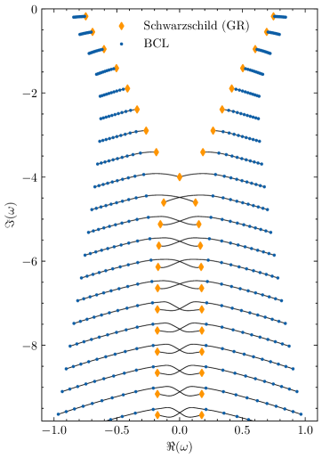
Figure 1: Axial quasinormal mode spectrum of the BCL black hole, for $\lambda=2$ and $r_{+}=1$. The parameter $r_{-}$ varies between 0 (Schwarzschild case, represented by diamonds) and 0.5. Blue dots correspond to increments of $0.05$ to the value of $r_{-}$.

We observe that higher-overtone modes are much more sensitive to small variations of $r_{-}$ (and thus to deviations from GR) even though this does not seem to come from a spectral instability Jaramillo:2020tuu here. For high overtones, the QNM points appear to be aligned along a straight line which, in contrast with the Schwarzschild case, is no longer vertical when $r_{-}\neq 0$. We can check that modes of much higher overtone still follow the same line, which seems to indicate that it corresponds to a real asymptote of the QNM spectrum. We have not been able to find an analytical argument to explain this behaviour. On figure 2, we illustrate the existence of such an asymptote at high overtones, which can be parametrised by the equation

$$\imaginary(\omega)=a\times\real(\omega)+b\,.$$ (54)

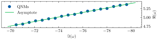
Figure 2: Asymptote of the QNM spectrum for $\lambda=2$, $r_{+}=1$ and $r_{-}=0.5$. The real and imaginary axes are rotated by 90 degrees compared to figure 1 for the sake of clarity.

The dependence on $r_{-}$ of the slope of the asymptote is shown in figure 3. The Schwarzschild case $r_{-}=0$ corresponds to a vertical asymptote with $1/a=0$. As $r_{-}$ becomes larger, the asymptote is less and less vertical.

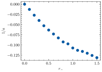
Figure 3: Inverse of the slope $a$ of the asymptote for $r_{+}=1$ and $\lambda=2$. Values of $r_{-}$ span between 0 (Schwarzschild case where the asymptote is vertical and $1/a=0$) and 1.5, with increments of 0.1.

As a final remark, we recall that the Schwarzschild QNM spectrum is well-known to contain special modes which have a vanishing real part, meaning they are purely-damped (non-oscillating) modes. They are associated with an “algebraically special” solution of the perturbation equations, obtained in chandrasekharAlgebraicallySpecialPerturbations1997 , and linked to the Robinson-Trautman metric describing nonperturbative gravitational waves onto a Schwarzschild background Qi:1993ey . When $\ell=2$, there is one such mode which corresponds to the overtone $n=8$ on figure 1. In the case of the BCL black hole, one sees that the mode of overtone $n=8$ is no longer purely-damped: as $r_{-}$ becomes non-zero, this mode splits into two modes of positive and negative real parts. Nevertheless, one can see that every subsequent mode moves towards the imaginary axis when $r_{-}$ increases and, for some critical value of $r_{-}$, reaches this axis. As a consequence, for some particular values of $r_{-}$, algebraically special modes still exist for the BCL black hole.

V Consistency checks

The numerical resolution of (33) requires a truncation of the recurrence relations at some finite rank $N$ (34). Such a truncation enables us to compute the matrices $R_{n}$ for any $n\leq N$ and then to solve (33).

V.1 Convergence of the method when $N$ increases

As a first consistency check, we need to make sure that the QNM frequencies thus computed converge towards a fixed value when $N$ increases. This is shown on figure 4 where we plot the difference between the computed QNM value $\omega$ in the Schwarzschild case ($r_{-}=0$) of axial perturbations and the known value $\omega_{*}$ computed in Berti:2009kk . We study several values of the overtone $n$. We observe that as $N$ increases, all modes converge to their theoretical value; however, higher overtones need higher values of $N$ to reach a good precision.

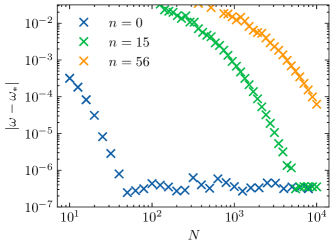
Figure 4: Convergence of the computed QNM frequencies, for different overtones. The convergence threshold is set at $10^{-6}$, which explains why the convergence does not improve beyond this value.

V.2 QNM mode functions

Given a value $\omega$ in the QNM spectrum, it is possible to perform a self-consistency check by computing $f_{0}$ and $f_{1}$ in (52) and verifying that the resulting functions solve the perturbation equations with the required boundary conditions as expected.

To see this is indeed the case, we first reformulate the perturbation equations in terms of $f_{0}$ and $f_{1}$. Hence, we substitute the ansatz (50) into the original perturbation equations (45-46), and we obtain that $f_{0}$ and $f_{1}$ must satisfy

$$\mathcal{E}_{0} \equiv g_{0}^{\prime}(r)+\kappa_{1}(r)g_{0}(r)+\kappa_{2}(r)g_{1}(r)=0\,,$$

$$\mathcal{E}_{1} \equiv g_{1}^{\prime}(r)+\kappa_{3}(r)g_{0}(r)+\kappa_{4}(r)g_{1}(r)=0\,,$$ (55)

where $g_{i}(r)=f_{i}(u(r))$ and the functions $\kappa_{i}$ are given by

$$\kappa_{1}(r) =\frac{1}{r}\quantity[-1+i\omega\quantity(r-r_{-}+r_{+}-\frac{r_{+}^{2}r_{0}}{r-r_{+}})]\,,$$

$$\kappa_{2}(r) =\frac{ir\omega}{r-r_{+}}-2i\lambda\frac{r+r_{-}}{r^{3}\omega}\,,$$

$$\kappa_{3}(r) =\frac{ir(r^{2}+2r_{+}r_{-})}{(r-r_{+})(r+r_{-})^{2}}\,,$$

$$\kappa_{4}(r) =\frac{1}{r+r_{-}}+i\omega\quantity[1+\frac{1}{r}\quantity(r_{+}-r_{-}-\frac{r_{+}^{2}r_{0}}{r-r_{+}})]\,.$$ (56)

We recall that the constants $r_{\pm}$ and $r_{0}$ are defined in (39) and in (49), respectively. Once we have these equations, we wish to check that, when $\omega$ belongs to the QNM spectrum, the functions $f_{0}$ and $f_{1}$ obtained numerically are indeed solutions. We perform two tests: first we pick up a frequency which is not a QNM and then we compare to the case where $\omega$ belongs to the spectrum.

Let us start by considering an arbitrary value of $\omega$. We compute the coefficients $a_{n}$ and $b_{n}$ and truncate the power series in (19) at some order $M$. We plot in figure 5 the values of $a_{n}$ and $b_{n}$ and see that they do not tend to zero, but on the contrary seem to diverge, which implies that the series  (19) are ill-defined. Furthermore, whereas equations $\mathcal{E}_{0}=0$ and $\mathcal{E}_{1}=0$ are verified close to the horizon, which is consistent with the fact that the power series decomposition of $f$ is done with respect to the variable $u=\ifrac{(r-r_{+})}{r}$, while at high values of $r$, the equations are clearly not satisfied very far from zero as $\mathcal{E}_{0}$ and $\mathcal{E}_{1}$ reach a constant value . As a consequence, when $\omega$ is not a QNM frequency, the numerical method does not lead to a solution for $f_{0}$ and $f_{1}$.

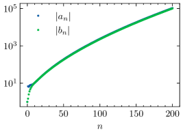
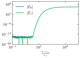
Figure 5: Absolute value of the coefficients $a_{n}$ and $b_{n}$ along with the absolute value of equations $\mathcal{E}_{0}$ and $\mathcal{E}_{1}$ for $r_{+}=1$, $r_{-}=0.2$, $\lambda=2$ and $\omega=0.5-0.3i$. The truncation is taken at $M=200$.

Let us now study the situation where $\omega$ belongs to the QNM spectrum. As an example, we take the fundamental mode $\omega_{0}$ for $\ell=2$ when $r_{-}=0.2$. The numerical calculation gives

$$\omega_{0}=0.785460-0.184148i\,\quad\text{or}\quad\,\omega_{0}=0.78546018859393-0.18414793488781i\,,$$ (57)

when the convergence threshold is put at $10^{-6}$ or at $10^{-14}$ respectively. Then, we compute the coefficients $a_{n}$ and $b_{n}$ for these two different precisions. The results are plotted in figure 6. We see that the first coefficients do seem to converge to zero, at least up to a certain value of $n$ represented by a dotted vertical line. As the accuracy of the mode increases, the convergence of the sequences $a_{n}$ and $b_{n}$ improves. Henceforth, we should truncate the sequence at the point where the coefficients start diverging: this means that with 6-digit accuracy, we should take $M\simeq 20$ while using 14-digit accuracy, we should use $M\simeq 100$.

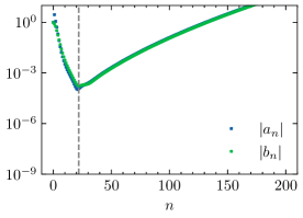
(a) 6-digits accuracy

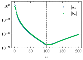
(b) 14-digits accuracy

Figure 6: Absolute values of the coefficients $a_{n}$ and $b_{n}$ for $r_{+}=1$, $r_{-}=0.2$, $\lambda=2$ and $\omega=\omega_{0}$. We consider two cases: in 6(a), we compute the value of $\omega_{0}$ up to 6 decimals and in 6(b), we compute it up to 14 decimals. In both cases, the truncation is taken at $M=200$. The vertical dotted line corresponds to threshold values of $n$ above which the coefficients do not seem to converge to zero anymore.

Finally we evaluate $\mathcal{E}_{0}$ and $\mathcal{E}_{1}$ to see whether the two series are indeed solutions of the equations. As in the previous case, these two equations are satisfied near the horizon. It is more interesting to look at these equations in the limit $r\rightarrow\infty$ where both equations converge towards a constant value at infinity similarly to what was seen in figure 5 for a non-QNM value of $\omega$. Furthermore, we notice that the asymptotic values for $\absolutevalue{\mathcal{E}_{0}}$ and $\absolutevalue{\mathcal{E}_{1}}$ are very close, and then we define $\mathcal{E}_{\infty}$ by

$$\mathcal{E}_{\infty}=\lim_{r\to\infty}\absolutevalue{\mathcal{E}_{0}}\simeq\lim_{r\to\infty}\absolutevalue{\mathcal{E}_{1}}\,.$$ (58)

On figure 7, we plot the values of $\mathcal{E}_{\infty}$ for different truncation values $M$. We find that, at low truncation rank $M$, $\mathcal{E}_{\infty}$ decreases with $M$ and reaches very low values. This means that the equations are solved and the value of $\omega$ is indeed a QNM. At higher values of $M$ however, equations do not seem to converge to zero anymore: this is because the sequences of coefficients $a_{n}$ and $b_{n}$ have stopped converging (as one can see in figure 6). What is important is that this threshold on $M$ increases as the precision on the QNM gets better: an arbitrarily high precision on the QNM frequency would lead to fully converging series of $a_{n}$ and $b_{n}$, and therefore a monotonous behaviour of $\mathcal{E}_{\infty}$.

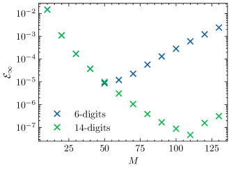
Figure 7: Values of $\mathcal{E}_{\infty}$ for $r_{+}=1$, $r_{-}=0.2$, $\lambda=2$ and $\omega=\omega_{0}$, for varying values of the truncation. We see that values decrease as $M$ increases, which means that the perturbation equations are verified. When $M$ becomes too high, convergence stops. We see that this threshold on $M$ increases with the precision sought for the NM value: as the precision increases, the threshold also increases.

In conclusion, we have shown that the QNM frequency $\omega$ computed with our method is associated with mode functions that do obey the perturbation equations (55). As the truncation value of the series (19) increases, we have checked that equations $\mathcal{E}_{0}$ and $\mathcal{E}_{1}$ get closer to zero, at least up to a threshold determined by the accuracy with which the QNM frequency was computed. This constitutes a strong self-consistency check of our method.

V.3 Initial coefficient vs. boundary condition at the horizon

Each QNM computed is such that the determinant of $\tilde{\alpha}_{0}R_{0}+Q_{0}$ is zero, which means that this matrix admits at least one null direction $Y_{0}$ (28). However, $Y_{0}$ is not arbitrary and it has been fixed by the asymptotic behaviour of the differential system at the horizon, given by (51) for the BCL black hole, which leads to

$$Y_{0}\propto\begin{pmatrix}r_{+}\\ r_{0}\end{pmatrix}\,.$$ (59)

In order to check this property, we compute a null vector $U$ of $\tilde{\alpha}_{0}R_{0}+Q_{0}$ for each QNM we have identified. To compare the directions of $U$ and $Y_{0}$, we compute their determinant or, equivalently, the quantity $\eta$ defined by

$$\eta=\frac{U_{1}}{U_{0}}-\frac{r_{0}}{r_{+}}\,.$$ (60)

The results are given in table (2) for different QNMs and different BH parameters. One can observe that the numerical vector $U$ is colinear with theoretical null vector $Y_{0}$, which is another strong indication of the consistency of our method. Notice however that the agreement worsens as the overtone increases. Interestingly, it has been observed (see Leaver:1985ax ) that solving the equation

$$\det(\tilde{\alpha}_{m}R_{m}+Q_{m})=0$$ (61)

for $m>0$ gives a better precision for the computation of the overtone $m$. Then, in order to have a good precision for high overtones, one should instead solve (61) for the corresponding value of $m$.

$\bm{n}$	$\bm{\eta}$
0	$1.1\text{\times}{10}^{-6}$
1	$1.5\text{\times}{10}^{-6}$
2	$4.3\text{\times}{10}^{-6}$
3	$3.8\text{\times}{10}^{-6}$
4	$1.2\text{\times}{10}^{-5}$
5	$3.4\text{\times}{10}^{-5}$
6	$6.2\text{\times}{10}^{-5}$
7	$1.9\text{\times}{10}^{-4}$
8	$2.0\text{\times}{10}^{-4}$
9	$3.0\text{\times}{10}^{-5}$

$\bm{n}$	$\bm{\eta}$
0	$9.9\text{\times}{10}^{-7}$
1	$2.9\text{\times}{10}^{-6}$
2	$7.1\text{\times}{10}^{-6}$
3	$7.8\text{\times}{10}^{-6}$
4	$2.1\text{\times}{10}^{-5}$
5	$3.9\text{\times}{10}^{-5}$
6	$6.3\text{\times}{10}^{-5}$
7	$2.3\text{\times}{10}^{-4}$
8	$3.9\text{\times}{10}^{-4}$
9	$4.3\text{\times}{10}^{-4}$

$\bm{n}$	$\bm{\eta}$
0	$8.7\text{\times}{10}^{-7}$
1	$2.6\text{\times}{10}^{-6}$
2	$4.6\text{\times}{10}^{-6}$
3	$1.2\text{\times}{10}^{-5}$
4	$1.8\text{\times}{10}^{-5}$
5	$3.7\text{\times}{10}^{-5}$
6	$8.1\text{\times}{10}^{-5}$
7	$2.1\text{\times}{10}^{-4}$
8	$5.0\text{\times}{10}^{-4}$
9	$6.5\text{\times}{10}^{-4}$

Table 2: Value of $\eta$ for $r_{-}=0$ (left), $r_{-}=0.25$ (middle) and $r_{-}=0.5$ (right). We have fixed $r_{+}=1$, $\lambda=2$, $N=1000$. We solved the equation (61) for $m=0$.

VI Discussion and conclusions

In the present work, we have implemented a numerical computation of the QNM frequencies based on the first-order form of the BH perturbation equations, using a matrix continued fraction method. To apply this method, an important ingredient is the knowledge of the asymptotic behaviours of the modes near the BH horizon and at spatial infinity. This information is obtained by using our previous works which provided an algorithm that can systematically identify the asymptotics of such first-order systems.

Here, we have applied our method to the Schwarzschild case, using the first-order form of the GR perturbed equations rather than the second-order Schrödinger equation, as a way to check the validity of this new approach, qualitatively and quantitatively. We have indeed verified that the Schwarzschild QNMs can be obtained in this way with a high precision.

We have then used the same method to compute, for the first time, the QNM frequencies of an exact BH solution obtained in a particular Horndeski theory. Interestingly, since the BH solution depends on a parameter that quantifies the deviation from the Schwarzschild solution, we can visualise the migration, in the complex plane, of the initial Schwarzschild QNMs as this parameter is increased. To check the robustness of our numerical results, we have performed various tests and compare our results with those based on other techniques.

For simplicity, we have restricted the present work to axial perturbations, where the scalar field perturbation vanishes, so that there is only one degree of freedom as in GR, even if the equations of motion are different. In this case, the recurrence relation involves matrices defined in a 2-dimensional vector space. Since this system can be easily rewritten in a second-order Schrödinger-like equation, we were able to check the accuracy of our numerical method versus existing methods that rely on such a reformulation. This constitutes a proof of concept for our numerical method, confirming that it gives high-precision results.

Moreover, our method should be readily applicable to a first-order system of any dimension. In particular, we expect the same technique to be applicable to polar perturbations, which contain the scalar field perturbation in addition to one gravitational mode, leading to a recurrence relation defined in a 4-dimensional space. We plan to pursue this in future work.

Beyond the specific numerical techniques used to compute the quasi-normal of a specific solutions, let us mention that recent discussions have raised interesting questions concerning the so-called spectral instability Jaramillo:2020tuu ; Jaramillo:2021tmt ; Destounis:2021lum ; Konoplya:2022pbc . Indeed, it has been observed that, under some hypotheses, a “small-scale” deviation from General Relativity could lead to a “large” deviation of the overtones, not necessary of very high (complex) frequency. These observations question the relevance of using QNM to test deviations from GR in the ringdown, even though the deviation is very “small”. However, in the case of the BCL Black Hole, we do not see such an instability: overtones deviate from the ones of Schwarzschild but in a linear controlled manner. Hence, it would be interesting to understand why some deviations lead indeed to a spectral instability and why others do not.

Appendix A recurrence relation for the BCL black hole

The matrix coefficients entering the 5-term recurrence relation (53) that we have obtained for the BCL black hole are given by

$$\alpha_{n} =\begin{pmatrix}\frac{n+1-ir_{0}\omega}{r_{+}}&i\omega\\ ir_{+}(2r_{-}+r_{+})\omega&(r_{+}+r_{-})^{2}\frac{n+1-ir_{0}\omega}{r_{+}}\end{pmatrix}\,,\quad\beta_{n}=\begin{pmatrix}\frac{-2n-1+i\omega(2r_{+}+2r_{0}-r_{-})}{r_{+}}&-\frac{2i\lambda(r_{+}+r_{-})}{r_{+}^{3}\omega}\\ -4ir_{+}r_{-}\omega&\beta_{22}\end{pmatrix}\,,$$

$$\gamma_{n} =\begin{pmatrix}\frac{n-i\omega(r_{+}+r_{0}-r_{-})}{r_{+}}&\frac{2i\lambda(2r_{+}+3r_{-})}{r_{+}^{3}\omega}\\ 2ir_{+}r_{-}\omega&\gamma_{22}\end{pmatrix}\,,\quad\delta_{n}=\begin{pmatrix}0&-\frac{2i\lambda(r_{+}+3r_{-})}{r_{+}^{3}\omega}\\ 0&\delta_{22}\end{pmatrix}\,,$$

$$\varepsilon_{n} =\begin{pmatrix}0&\frac{2i\lambda r_{-}}{r_{+}^{3}\omega}\\ 0&\frac{r_{-}^{2}}{r_{+}}\quantity[n-3-i\omega(r_{+}+r_{0}-r_{-})]\end{pmatrix}\,.$$

The expressions of the coefficients $\beta_{22}$, $\gamma_{22}$ and $\delta_{22}$ are given by

$$\beta_{22} = \frac{r_{+}+r_{-}}{r_{+}}\quantity[-2n(2r_{-}+r_{+})+r_{+}+i\omega(2r_{+}^{2}+r_{+}(2r_{0}+r_{-})+r_{-}(4r_{0}-r_{-}))],$$

$$\gamma_{22} = \frac{3ir_{-}^{3}\omega}{r_{+}}+\frac{r_{-}^{2}}{r_{+}}\quantity[6(n-1)-i\omega(r_{+}+6r_{0})]+r_{-}\quantity[6n-8-i\omega(5r_{+}+6r_{0})]+r_{+}\quantity[n-2-i\omega(r_{+}+r_{0})],$$

$$\delta_{22} = \frac{r_{-}}{r_{+}}\quantity[-2n(r_{+}+2r_{-})+5r_{+}+8r_{-}+i\omega(-3r_{-}^{2}+2r_{+}(r_{0}+r_{+})+2r_{-}(2r_{0}+r_{+}))]\,.$$

One recovers the coefficients for the Schwarzschild recurrence relation given in (22) in the limit $r_{+}=\mu$ and $r_{-}=0$.

Appendix B Gaussian reduction for a 5-term recurrence relation

In this appendix, we describe the Gaussian reduction procedure that enables us to reduce the five-term recurrence relation (53) into a three-term recurrence relation of the form (23). We give a proof by induction. Let us assume that there exists $p\geq 3$ such that the five-term recurrence relation (53) for all $n\leq p$ can be equivalently reformulated into the form

$$\tilde{\alpha}_{n}Y_{n+1}+\tilde{\beta}_{n}Y_{n}+\tilde{\gamma}_{n}Y_{n-1}=0\,,$$ (62)

for all $n\leq p$ as well. Then, we want to prove that it is possible to cast the next order,

$$\alpha_{p+1}Y_{p+2}+\beta_{p+1}Y_{p+1}+\gamma_{p+1}Y_{p}+\delta_{p+1}Y_{p-1}+\varepsilon_{p+1}Y_{p-2}=0\,,$$ (63)

into a similar form.

The first step consists in using (62) at order $p-1$,

$$\tilde{\alpha}_{p-1}Y_{p}+\tilde{\beta}_{p-1}Y_{p-1}+\tilde{\gamma}_{p-1}Y_{p-2}=0\,.$$ (64)

If we assume $\tilde{\gamma}_{p-1}$ to be invertible, we can eliminate $Y_{p-2}$ in (63) and we obtain,

$$\alpha_{p+1}Y_{p+2}+\beta_{p+1}Y_{p+1}+\big{(}\gamma_{p+1}-\varepsilon_{p+1}\cdot\tilde{\gamma}_{p-1}^{-1}\cdot\tilde{\alpha}_{p-1}\big{)}Y_{p}+\big{(}\delta_{p+1}-\varepsilon_{p+1}\cdot\tilde{\gamma}_{p-1}^{-1}\cdot\tilde{\beta}_{p-1}\big{)}Y_{p-1}=0\,.$$ (65)

Now, we use once more (62) but now at order $p$ so that we can express $Y_{p-1}$ in terms of $Y_{p}$ and $Y_{p+1}$ assuming that $\tilde{\gamma}_{p}$ is invertible. Hence, after a direct calculation, we end up with the 3-term recurrence relation,

$$\alpha_{p+1}Y_{p+2}+\Big{[}\beta_{p+1}-\big{(}\delta_{p+1}-\varepsilon_{p+1}\cdot\tilde{\gamma}_{p-1}^{-1}\cdot\tilde{\beta}_{p-1}\big{)}\cdot\tilde{\gamma}_{p}^{-1}\cdot\tilde{\alpha}_{p}\Big{]}Y_{p+1}\\ +\Big{[}\big{(}\gamma_{p+1}-\varepsilon_{p+1}\cdot\tilde{\gamma}_{p-1}^{-1}\cdot\tilde{\alpha}_{p-1}\big{)}-\big{(}\delta_{p+1}-\varepsilon_{p+1}\cdot\tilde{\gamma}_{p-1}^{-1}\cdot\tilde{\beta}_{p-1}\big{)}\cdot\tilde{\gamma}_{p}^{-1}\cdot\tilde{\beta}_{p}\Big{]}Y_{p}=0\,.$$ (66)

Finally, as the hypothesis (62) is true for any $n\leq 3$ (i.e. for $p=3$), the five-term recurrence relation can be equivalently reformulated as (62) for any $n$. Furthermore, the new matrix coefficients $\tilde{\alpha}_{n+1}$, $\tilde{\beta}_{n+1}$ and $\tilde{\gamma}_{n+1}$ can be computed recursively from

$$\tilde{\alpha}_{n+1} =\alpha_{n+1}\,,$$ (67)

$$\tilde{\beta}_{n+1} =\beta_{n+1}-\big{(}\delta_{n+1}-\varepsilon_{n+1}\cdot\tilde{\gamma}_{n-1}^{-1}\cdot\tilde{\beta}_{n-1}\big{)}\cdot\tilde{\gamma}_{n}^{-1}\cdot\tilde{\alpha}_{n}\,,$$ (68)

$$\tilde{\gamma}_{n+1} =\big{(}\gamma_{n+1}-\varepsilon_{n+1}\cdot\tilde{\gamma}_{n-1}^{-1}\cdot\tilde{\alpha}_{n-1}\big{)}-\big{(}\delta_{n+1}-\varepsilon_{n+1}\cdot\tilde{\gamma}_{n-1}^{-1}\cdot\tilde{\beta}_{n-1}\big{)}\cdot\tilde{\gamma}_{n}^{-1}\cdot\tilde{\beta}_{n}\,.$$ (69)

Appendix C Comparison with other methods

In order to further verify the authenticity of the computed QNMs, it is important to compare their value outside of the Schwarzschild limit $r_{-}=0$. However, until now, there has been no investigation of the QNMs of the BCL black hole in the literature. Therefore, we adapt existing methods to the case of this black hole and compare the results obtained.

In the following, we use the fact that axial perturbations of the BCL black hole can be cast into the Schrödinger-like form Langlois:2021aji

$$-\derivative[2]{\Psi}{r_{*}}+(V(r)-\omega^{2})\Psi=0\,,$$ (70)

with the potential given by

$$V(r)=\frac{(r-r_{+})(r+r_{-})}{r^{4}(r^{2}+2r_{+}r_{-})^{3}}\times\sum_{k=0}^{6}p_{k}r^{k}\,,$$ (71)

where the coefficients $p_{k}$ are given by

$$p_{0} =r_{+}^{3}r_{-}^{3}(16\lambda-5)\,, p_{1} =3r_{+}^{2}r_{-}^{2}(r_{-}-r_{+})\,, p_{2} =6r_{+}^{2}r_{-}^{2}(4\lambda-1)\,,$$

$$p_{3} =4r_{+}r_{-}(r_{-}-r_{+})\,, p_{4} =3r_{+}r_{-}(4\lambda-1)\,, p_{5} =3(r_{-}-r_{+})\,,$$

$$p_{6} =2(\lambda+1)\,.$$ (72)

The tortoise coordinate $r_{*}$ is defined such that

$$\derivative{r_{*}}{r}=\frac{1}{A(r)}\,,$$ (73)

with $A(r)$ given in (38).

C.0.1 WKB method

The WKB method allows one to compute QNMs by approximating the potential $V$ near its maximum. It was proposed originally in Schutz:1985km , improved in Iyer:1986np ; Iyer:1986nq and further improved in Konoplya:2003ii ; Matyjasek:2017psv (see Konoplya:2019hlu for a review). The results of Iyer:1986nq , sufficient for our computation, can be summed up as follows: if the potential $V$ seen as a function of $r_{*}$ has a maximum at $r_{*}=r_{*0}$, then one can decompose the potential as

$$V(r_{*})=V_{0}+\frac{1}{2}V_{0}^{(2)}(r_{*}-r_{*0})^{2}+...=V_{0}+\sum_{k=2}^{+\infty}\frac{1}{k!}V_{0}^{(k)}(r_{*}-r_{*0})^{k}\,.$$ (74)

If one truncates the decomposition of (74) at order 6, then the QNMs $\omega_{n}$ are given by the solutions of

$$\omega_{n}^{2}=\quantity(V_{0}+\sqrt{-2V_{0}^{(2)}}\Lambda)-i\quantity(n+\frac{1}{2})\sqrt{-2V_{0}^{(2)}}(1+\Omega)\,,$$ (75)

where $\Lambda$ and $\Omega$ are functions of $V_{0}^{(2)},...,V_{0}^{(6)}$ whose expressions are given in Iyer:1986nq .

Equation (75) can then be solved for $\omega_{n}$. In table 3, we compare the QNM values obtained via the matrix continued fraction method and the WKB method for a nonzero $r_{-}$.

$\bm{n}$	Matrix continued fraction	WKB method
0	0.843719 - 0.197227i	0.843204 - 0.19805i
1	0.794262 - 0.607533i	0.793898 - 0.60744i
2	0.720858 - 1.059862i	0.715865 - 1.03543i
3	0.661666 - 1.556088i	0.615373 - 1.47301i
4	0.632640 - 2.077741i	0.490639 - 1.91668i
5	0.627338 - 2.610898i	0.340383 - 2.36668i
6	0.636227 - 3.149321i	0.164472 - 2.82404i

Table 3: Comparison between the first QNM values obtained via our numerical method and the WKB approximation, for $\lambda=2$, $r_{+}=1$, $r_{-}=0.5$.

We observe that the first overtones are very well approximated by the WKB method while this method fails at higher values of $n$.

C.0.2 Spectral decomposition

We can also compare our QNM computation with another fully numerical computation, based on the numerical resolution of the Schrödinger-like reformulation of the axial perturbations equations. This method was developed in Jansen:2017oag and relies on a spectral decomposition of the mode function in order to cast the QNM computation problem into a generalized eigenvalue problem. It is available as a Mathematica package and only requires the Schrödinger-like equation (70) and the potential (71), rescaled in an appropriate way.

In table 4, we compare the QNM values obtained via the matrix continued fraction method and this numerical method (called QNMSpectral) for a non-zero $r_{-}$.

$\bm{n}$	Matrix continued fraction	QNMSpectral method
0	0.84371827443 - 0.19722719264i	0.84371827438 - 0.19722719255i
1	0.79426238123 - 0.60753311430i	0.79426237852 - 0.60753340736i
2	0.72085805503 - 1.05986135470i	0.72088369854 - 1.05978730679i

Table 4: Comparison between the first QNM values obtained via our numerical method and the QNMSpectral numerical routine, for $\lambda=2$, $r_{+}=1$, $r_{-}=0.5$.

We observe that both methods agree up to a very high precision on the first overtones (we used a convergence threshold of $10^{-14}$ to account for this). However, it is not possible to reach higher values of $n$ using the QNMSpectral approach (and this method requires a Schrödinger-like reformulation, which is not available for polar perturbations).

References

- (1) D. Langlois and K. Noui, “Degenerate higher derivative theories beyond Horndeski: Evading the Ostrogradski instability,” Journal of Cosmology and Astroparticle Physics 2016 (Feb., 2016) 034–034, 1510.06930.
- (2) D. Langlois and K. Noui, “Hamiltonian analysis of higher derivative scalar-tensor theories,” JCAP 1607 (2016), no. 07 016, 1512.06820.
- (3) J. Ben Achour, D. Langlois, and K. Noui, “Degenerate higher order scalar-tensor theories beyond Horndeski and disformal transformations,” Physical Review D 93 (June, 2016) 124005, 1602.08398.
- (4) M. Crisostomi, K. Koyama, and G. Tasinato, “Extended Scalar-Tensor Theories of Gravity,” Journal of Cosmology and Astroparticle Physics 2016 (Apr., 2016) 044–044, 1602.03119.
- (5) J. Ben Achour, M. Crisostomi, K. Koyama, D. Langlois, K. Noui, and G. Tasinato, “Degenerate higher order scalar-tensor theories beyond Horndeski up to cubic order,” Journal of High Energy Physics 2016 (Dec., 2016) 100, 1608.08135.
- (6) David Langlois, “Dark Energy and Modified Gravity in Degenerate Higher-Order Scalar-Tensor (DHOST) theories: A review,” International Journal of Modern Physics D 28 (Apr., 2019) 1942006, 1811.06271.
- (7) T. Kobayashi, “Horndeski theory and beyond: A review,” Reports on Progress in Physics 82 (Aug., 2019) 086901, 1901.07183.
- (8) E. Babichev, C. Charmousis, and A. Lehébel, “Asymptotically flat black holes in Horndeski theory and beyond,” Journal of Cosmology and Astroparticle Physics 2017 (Apr., 2017) 027–027, 1702.01938.
- (9) J. Ben Achour and H. Liu, “Hairy Schwarzschild-(A)dS black hole solutions in DHOST theories beyond shift symmetry,” Physical Review D 99 (Mar., 2019) 064042, 1811.05369.
- (10) H. Motohashi and M. Minamitsuji, “Exact black hole solutions in shift-symmetric quadratic degenerate higher-order scalar-tensor theories,” Physical Review D 99 (Mar., 2019) 064040, 1901.04658.
- (11) C. Charmousis, M. Crisostomi, R. Gregory, and N. Stergioulas, “Rotating Black Holes in Higher Order Gravity,” Physical Review D 100 (Oct., 2019) 084020, 1903.05519.
- (12) M. Minamitsuji and J. Edholm, “Black hole solutions in shift-symmetric degenerate higher-order scalar-tensor theories,” Physical Review D100 (2019), no. 4 044053, 1907.02072.
- (13) J. Ben Achour, H. Liu, and S. Mukohyama, “Hairy black holes in DHOST theories: Exploring disformal transformation as a solution-generating method,” JCAP 02 (2020) 023, 1910.11017.
- (14) M. Minamitsuji and J. Edholm, “Black holes with a nonconstant kinetic term in degenerate higher-order scalar tensor theories,” Physical Review D101 (2020), no. 4 044034, 1912.01744.
- (15) T. Anson, E. Babichev, C. Charmousis, and M. Hassaine, “Disforming the kerr metric,” JHEP 01 (2021) 018, 2006.06461.
- (16) J. Ben Achour, H. Liu, H. Motohashi, S. Mukohyama, and K. Noui, “On rotating black holes in DHOST theories,” JCAP 11 (2020), no. references numbers: YITP-20-81, IPMU20-0067 001, 2006.07245.
- (17) K. Takahashi and H. Motohashi, “General Relativity solutions with stealth scalar hair in quadratic higher-order scalar-tensor theories,” Journal of Cosmology and Astroparticle Physics 2020 (June, 2020) 034–034, 2004.03883.
- (18) E. Babichev, C. Charmousis, A. Cisterna, and M. Hassaine, “Regular black holes via the Kerr-Schild construction in DHOST theories,” JCAP 06 (2020) 049, 2004.00597.
- (19) O. Baake, M. F. Bravo Gaete, and M. Hassaine, “Spinning black holes for generalized scalar tensor theories in three dimensions,” Physical Review D: Particles and Fields 102 (2020), no. 2 024088, 2005.10869.
- (20) L. Capuano, L. Santoni, and E. Barausse, “Black hole hairs in scalar-tensor gravity and the lack thereof,” Physical Review D 108 (Sept., 2023) 064058, 2304.12750.
- (21) A. Bakopoulos, C. Charmousis, P. Kanti, N. Lecoeur, and T. Nakas, “Black holes with primary scalar hair,” 2310.11919.
- (22) E. Babichev, C. Charmousis, and N. Lecoeur, “Exact black hole solutions in higher-order scalar-tensor theories,” 2309.12229.
- (23) K. D. Kokkotas and B. G. Schmidt, “Quasi-Normal Modes of Stars and Black Holes,” Living Reviews in Relativity 2 (1999), no. 1 gr-qc/9909058.
- (24) H.-P. Nollert, “Quasinormal modes: The characteristic ’sound’ of black holes and neutron stars,” Classical and Quantum Gravity 16 (Nov., 1999) R159–R216.
- (25) E. Berti, V. Cardoso, and A. O. Starinets, “Quasinormal modes of black holes and black branes,” Classical and Quantum Gravity 26 (Aug., 2009) 163001, 0905.2975.
- (26) R. A. Konoplya and A. Zhidenko, “Quasinormal modes of black holes: From astrophysics to string theory,” Reviews of Modern Physics 83 (July, 2011) 793–836.
- (27) E. Berti, V. Cardoso, and C. M. Will, “On gravitational-wave spectroscopy of massive black holes with the space interferometer LISA,” Physical Review D 73 (Mar., 2006) 064030, gr-qc/0512160.
- (28) E. Berti, K. Yagi, H. Yang, and N. Yunes, “Extreme Gravity Tests with Gravitational Waves from Compact Binary Coalescences: (II) Ringdown,” General Relativity and Gravitation 50 (May, 2018) 49, 1801.03587.
- (29) L. Hui, A. Podo, L. Santoni, and E. Trincherini, “An analytic approach to quasinormal modes for coupled linear systems,” Journal of High Energy Physics 2023 (Mar., 2023) 60, 2210.10788.
- (30) P. Pani, “Advanced Methods in Black-Hole Perturbation Theory,” International Journal of Modern Physics A 28 (Sept., 2013) 1340018, 1305.6759.
- (31) N. Franchini and S. H. Völkel, “Testing General Relativity with Black Hole Quasi-Normal Modes,” 2305.01696.
- (32) E. W. Leaver and S. Chandrasekhar, “An analytic representation for the quasi-normal modes of Kerr black holes,” Proceedings of the Royal Society of London. A. Mathematical and Physical Sciences 402 (Jan., 1997) 285–298.
- (33) T. Regge and J. A. Wheeler, “Stability of a Schwarzschild Singularity,” Physical Review 108 (Nov., 1957) 1063–1069.
- (34) F. J. Zerilli, “Effective Potential for Even-Parity Regge-Wheeler Gravitational Perturbation Equations,” Physical Review Letters 24 (Mar., 1970) 737–738.
- (35) S. A. Teukolsky, “Perturbations of a rotating black hole. 1. Fundamental equations for gravitational electromagnetic and neutrino field perturbations,” Astrophysical Journal 185 (1973) 635–647.
- (36) D. Langlois, K. Noui, and H. Roussille, “Asymptotics of linear differential systems and application to quasi-normal modes of nonrotating black holes,” Physical Review D 104 (Dec., 2021) 124043, 2103.14744.
- (37) D. Langlois, K. Noui, and H. Roussille, “Black hole perturbations in modified gravity,” Physical Review D 104 (Dec., 2021) 124044, 2103.14750.
- (38) D. Langlois, K. Noui, and H. Roussille, “Linear perturbations of Einstein-Gauss-Bonnet black holes,” Journal of Cosmology and Astroparticle Physics 2022 (Sept., 2022) 019, 2204.04107.
- (39) J. L. Blázquez-Salcedo, C. F. B. Macedo, V. Cardoso, V. Ferrari, L. Gualtieri, F. S. Khoo, J. Kunz, and P. Pani, “Perturbed black holes in Einstein-dilaton-Gauss-Bonnet gravity: Stability, ringdown, and gravitational-wave emission,” Physical Review D 94 (Nov., 2016) 104024, 1609.01286.
- (40) J. L. Blázquez-Salcedo, F. S. Khoo, and J. Kunz, “Quasinormal modes of Einstein-Gauss-Bonnet-dilaton black holes,” Physical Review D: Particles and Fields 96 (2017), no. 6 064008, 1706.03262.
- (41) T. Kobayashi, H. Motohashi, and T. Suyama, “Black hole perturbation in the most general scalar-tensor theory with second-order field equations I: The odd-parity sector,” Physical Review D 85 (Apr., 2012) 084025, 1202.4893.
- (42) T. Kobayashi, H. Motohashi, and T. Suyama, “Black hole perturbation in the most general scalar-tensor theory with second-order field equations II: The even-parity sector,” Physical Review D 89 (Apr., 2014) 084042, 1402.6740.
- (43) W. Gautschi, “Computational Aspects of Three-Term Recurrence Relations,” SIAM Review 9 (Jan., 1967) 24–82.
- (44) C. Simmendinger, A. Wunderlin, and A. Pelster, “Analytical approach for the Floquet theory of delay differential equations,” Physical Review E 59 (May, 1999) 5344–5353.
- (45) J. G. Rosa and S. R. Dolan, “Massive vector fields on the Schwarzschild spacetime: Quasinormal modes and bound states,” Physical Review D 85 (Feb., 2012) 044043, 1110.4494.
- (46) G. W. Horndeski, “Second-order scalar-tensor field equations in a four-dimensional space,” Int.J.Theor.Phys. 10 (1974) 363–384.
- (47) J. L. Jaramillo, R. P. Macedo, and L. A. Sheikh, “Pseudospectrum and black hole quasi-normal mode (in)stability,” Physical Review X 11 (July, 2021) 031003, 2004.06434.
- (48) S. Chandrasekhar, “On algebraically special perturbations of black holes,” Proceedings of the Royal Society of London. A. Mathematical and Physical Sciences 392 (Jan., 1997) 1–13.
- (49) G. Qi and B. F. Schutz, “Robinson-Trautman equations and Chandrasekhar’s special perturbation of the Schwarzschild metric,” General Relativity and Gravitation 25 (Nov., 1993) 1185–1188.
- (50) J. L. Jaramillo, R. P. Macedo, and L. A. Sheikh, “Gravitational wave signatures of black hole quasi-normal mode instability,” Physical Review Letters 128 (May, 2022) 211102, 2105.03451.
- (51) K. Destounis, R. P. Macedo, E. Berti, V. Cardoso, and J. L. Jaramillo, “Pseudospectrum of Reissner-Nordström black holes: Quasinormal mode instability and universality,” Physical Review D 104 (Oct., 2021) 084091, 2107.09673.
- (52) R. A. Konoplya and A. Zhidenko, “First few overtones probe the event horizon geometry,” 2209.00679.
- (53) B. F. Schutz and C. M. Will, “Black hole normal modes - A semianalytic approach,” The Astrophysical Journal 291 (Apr., 1985) L33–L36.
- (54) S. Iyer and C. M. Will, “Black-hole normal modes: A WKB approach. I. Foundations and application of a higher-order WKB analysis of potential-barrier scattering,” Physical Review D 35 (June, 1987) 3621–3631.
- (55) S. Iyer, “Black-hole normal modes: A WKB approach. II. Schwarzschild black holes,” Physical Review D 35 (June, 1987) 3632–3636.
- (56) R. A. Konoplya, “Quasinormal behavior of the D-dimensional Schwarzshild black hole and higher order WKB approach,” Physical Review D 68 (July, 2003) 024018, gr-qc/0303052.
- (57) J. Matyjasek and M. Opala, “Quasinormal modes of black holes. The improved semianalytic approach,” Physical Review D 96 (July, 2017) 024011, 1704.00361.
- (58) R. A. Konoplya, A. Zhidenko, and A. F. Zinhailo, “Higher order WKB formula for quasinormal modes and grey-body factors: Recipes for quick and accurate calculations,” Classical and Quantum Gravity 36 (Aug., 2019) 155002, 1904.10333.
- (59) A. Jansen, “Overdamped modes in Schwarzschild-de Sitter and a Mathematica package for the numerical computation of quasinormal modes,” The European Physical Journal Plus 132 (Dec., 2017) 546, 1709.09178.