When Model Meets New Normals:
Test-Time Adaptation for Unsupervised Time-Series Anomaly Detection

Abstract

Time-series anomaly detection deals with the problem of detecting anomalous timesteps by learning normality from the sequence of observations. However, the concept of normality evolves over time, leading to a "new normal problem", where the distribution of normality can be changed due to the distribution shifts between training and test data. This paper highlights the prevalence of the new normal problem in unsupervised time-series anomaly detection studies. To tackle this issue, we propose a simple yet effective test-time adaptation strategy based on trend estimation and a self-supervised approach to learning new normalities during inference. Extensive experiments on real-world benchmarks demonstrate that incorporating the proposed strategy into the anomaly detector consistently improves the model’s performance compared to the baselines, leading to robustness to the distribution shifts.

Introduction

In real-world monitoring systems, the continuous operation of numerous sensors generates substantial real-time measurements. Time-series anomaly detection aims to identify observations that deviate from the concept of normality (Ruff et al. 2021; Pang et al. 2022) within a sequence of observations. Examples of anomalous events include physical attacks on industrial systems (Mathur and Tippenhauer 2016; Han et al. 2021), unpredictable robot behavior (Park, Hoshi, and Kemp 2018), faulty sensors from wide-sensor networks (Wang, Kuang, and Duan 2015; Rassam, Maarof, and Zainal 2018), cybersecurity attacks on server monitoring systems (Su et al. 2019; Abdulaal, Liu, and Lancewicki 2021), and spacecraft malfunctions based on telemetry sensor data (Hundman et al. 2018; Shin et al. 2020; Liu, Liu, and Peng 2016).

However, detecting abnormal timesteps presents significant challenges due to several factors. Firstly, the complex nature of system dynamics, characterized by the coordination of multiple sensors, complicates the task. Secondly, the increasing volume of incoming signals to monitoring systems adds to the difficulty. Lastly, acquiring labels for abnormal behaviors is problematic. To address these challenges, unsupervised time-series anomaly detection models (Xu et al. 2022; Audibert et al. 2020; Su et al. 2019; Park, Hoshi, and Kemp 2018; Malhotra et al. 2016) have emerged, focusing on learning normal patterns from available training datasets and being deployed after training.

Nevertheless, the concept of normality can change over time, widely known as a distribution shift (Quinonero-Candela et al. 2008; Kim et al. 2022b; Sun et al. 2020; Gulrajani and Lopez-Paz 2021; Wang et al. 2021, 2022), as can be seen in the Fig. 1-(a). We have observed that off-the-shelf models are susceptible to such shifts, leading to a "new normal problem", where the distribution of normality during test time cannot be fully characterized solely based on training data. Without consideration of distribution shifts, these models tend to rely on past observations and generate false alarms, compromising the consistency of monitoring systems (Dragoi et al. 2022; Cao, Zhu, and Pang 2023).

Figure 1: Motivation for learning new normals. (a) T-SNE visualization of the SWaT benchmark (Mathur and Tippenhauer 2016) reveals distinct behavior between the training (red) and test data (blue). (b) Our test-time adaptation strategy surpasses previous state-of-the-art time-series anomaly detection models in terms of F1 score, even with simple baselines such as MLP-based autoencoders. (c) This improvement arises from effectively handling significant distribution shifts in the time-series data. Over time, off-the-shelf models fail to adapt to these new normals, while our approach exhibits robustness to such distribution shifts. Consequently, previous approaches (Audibert et al. 2020; Shen, Li, and Kwok 2020) produce false positive cases due to the model’s inability to keep pace with changing dynamics, thereby "the model is staying in the past while the world is changing."

Recently, test-time adaptation mechanisms (Wang et al. 2021, 2022; Niu et al. 2022) have been proposed to adapt models for alleviating performance degradation due to distribution shifts between training and test datasets, especially in the computer vision field. Test-time adaptation methods update the model parameters to generalize to different data distributions, without relying on either additional supervision from labels or access to training data. Time-series anomaly detection task also shares motivation for applying test-time adaptation strategies; frequent access to past data for adaptation is costly as monitoring systems work in real-time (Abdulaal, Liu, and Lancewicki 2021; Shin et al. 2020; Su et al. 2019) and model update without supervision is desired as acquiring labels is often limited (Geiger et al. 2020; Ruff et al. 2021; Audibert et al. 2020). Motivated by these advancements, we propose a test-time adaptation for unsupervised time-series anomaly detection under distribution shifts.

Our paper highlights the prevalence of the new normal problem in time-series anomaly detection literature. To address this issue properly, we propose a simple yet effective adaptation strategy using trend estimates and model updates with normal instances based on the model’s prediction itself. Trend estimate, given by the exponential moving average of the observations, follows the expected value of a time-series with adaptation to changing conditions (Muth 1960) with computational efficiency. After model deployment, we update the model parameters with the normalized input sequence, which is detrended by subtracting the trend estimate, to learn complicated dynamics that cannot be captured solely on the trend estimate. Our proposed method makes the model robust to such distribution shifts, thereby increasing detector performance, as shown in Fig. 1-(b) and Fig. 1-(c).

Our contributions can be summarized as follows:

• We discover that new normal problems pose a significant challenge in modeling unsupervised time-series anomaly detection under distribution shifts.

• We propose a simple yet effective adaptation strategy following the trend estimate of the time-series data and update the model parameters using a detrended sequence to address these problems.

• Through extensive experiments on various real-world datasets, our method consistently improves the model’s performance when facing a severe distribution shift problem between training data and test data.

Related Works

Unsupervised time-series anomaly detection. Unsupervised time-series anomaly detection (Su et al. 2019; Audibert et al. 2020; Xu et al. 2022) aims to detect observations that deviate considerably from normality, assuming the non-existence of the available labels. To the extent of conventional anomaly detection approaches (Breunig et al. 2000; Schölkopf et al. 1999; Tax and Duin 1999) and deep-learning-based anomaly detection approaches (Zong et al. 2018; Ruff et al. 2018), unsupervised time-series anomaly detection models aim to build an architecture that can model the temporal dynamics of the sequence.

The main categories of unsupervised time-series anomaly detection models include reconstruction-based models, clustering-based models, and forecasting-based models. Building upon the assumption of better reconstruction performance of normal instances compared to anomalous instances, reconstruction-based models encompass a range of approaches involving LSTM (Malhotra et al. 2016; Park, Hoshi, and Kemp 2018; Su et al. 2019) and MLP (Audibert et al. 2020) architectures, as well as the integration of GANs (Schlegl et al. 2017; Geiger et al. 2020; Han et al. 2021). Clustering-based methods include the extension of one-class support vector machine approaches (Schölkopf et al. 1999; Tax and Duin 1999), tensor decomposition-based clustering methods for the detection of anomalies (Shin et al. 2020), and the utilization of latent representations for clustering (Ruff et al. 2018; Shen, Li, and Kwok 2020). Forecasting-based methods rely on detecting anomalies by identifying substantial deviations between past sequences and ground truth labels, as exemplified by the use of ARIMA (Pena, de Assis, and Jr. 2013), LSTM (Hundman et al. 2018), and transformer (Xu et al. 2022).

Figure 2: Illustration of the necessity for estimating trends and test-time adaptation. (a) NeurIPS-TS-UNI shows synthetic data generated based on the previous work (Lai et al. 2021), revealing an abrupt trend shift while preserving underlying dynamics. The objective of the trend estimation module is to adapt to such trend shifts successfully. (b) Solely relying on trend estimation may not be adequate to fully capture the dynamics, as demonstrated by the Yahoo-A1-R20 series. The shaded purple and yellow areas represent the standard deviations of the train and test data, respectively. To model this shift in dynamics, which cannot be fully captured alone with trend estimates, it is necessary to learn distribution shifts through test-time model updates outlined directly.

Distribution shift in time-series data. Due to the nature of continually changing temporal dynamics, mitigating distribution shifts emerges as a pivotal concern within the time-series data analysis, notably within tasks such as time-series forecasting (Kim et al. 2022b; Liu et al. 2022) and anomaly detection (Sankararaman et al. 2022; Dragoi et al. 2022).

Online RNN-AD (Saurav et al. 2018) adapts to concept drift with RNN architectures, which update the model with backpropagation of anomaly scores using all stream data. Our work differentiates from this work by introducing detrending modules for model updates and selective learning of a set of normal instances in a self-supervised way. Although recent work (Sankararaman et al. 2022) also presents an adaptable framework for anomaly detection, it hinges on a dynamic window mechanism applied to historical data streams. Notably, our approach diverges from their assumption of accessibility of past sequences; we keep model parameters at hand, process input sequences immediately, and evict after.

Test-time adaptation. To alleviate the performance degradation caused by distribution shift, unsupervised domain adaptation (Ganin et al. 2016; Zou et al. 2018; Yoo, Chung, and Kwak 2022; Liang, Hu, and Feng 2020) methods have been developed in various fields. These methods align with our work from the perspective of addressing the covariate shift problem. In recent times, fully test-time adaptation (TTA) (Wang et al. 2021) methods have emerged to enhance the model performance on test data through real-time adaptation using unlabeled test samples during inference, without relying on access to the training data. Most TTA approaches employ entropy minimization (Wang et al. 2021; Niu et al. 2022; Choi et al. 2022) or pseudo labels (Wang et al. 2022) to update the model parameters using unlabeled test samples. However, simply adopting previous TTA methods may not be directly applicable to unsupervised time-series anomaly detection. This is due to the vulnerability of the model when updating the model using all test samples, as abnormal test samples have the potential to disrupt its functionality. Consequently, this work aims to successfully apply the concept of test-time adaptation to the unsupervised time-series anomaly detection task.

Method

Problem Statement

Unsupervised time-series anomaly detection aims to detect anomalous timesteps during test time without explicit supervision by learning the concept of normality. The concept of normality is defined as the probability distribution $\mathbb{P}$ on data $\mathcal{D}$ that is the ground-truth law of normal behavior in a given task (Ruff et al. 2021). Accordingly, a set of anomalies is defined as data with sufficiently small probability under such distribution, i.e., $p(x)<\epsilon$. New normal problem that we tackle can be formulated as the phenomena of underlying distribution $\mathbb{P}$ is not stationary, i.e., $\mathbb{P}_{train}\neq\mathbb{P}_{test}$.

For observations over $N$ timesteps with $F$ features, time-series data is specified by a sequence $\mathcal{D}=\{X_{1},X_{2},...,X_{N}\}$, where each $X_{i}\in\mathbb{R}^{F}$. An anomaly detector aims to map each observation to a class label $y=\{0,1\}$, where $y=0$ and $y=1$ each denote normal and abnormal timesteps. The detector is specified by an anomaly score function $\mathcal{A}:\mathbb{R}^{F}\rightarrow\mathbb{R}$, along with a decision threshold $\tau$. Concretely, observation $X_{t}$ is classified as anomalous if $\mathcal{A}(X_{t})>\tau$. We denote the set of train-time instances as $\mathcal{D}_{train}$ and the set of test-time instances as $\mathcal{D}_{test}$. Accordingly, test-time normals and anomalies can be defined each as $\{X\in\mathcal{D}_{test}\ |\ y=0\}$ and $\{X\in\mathcal{D}_{test}\ |\ y=1\}$.

To reflect the temporal context of time-series data to detect anomalous timestep(s), a set of observations $\mathcal{D}$ is preprocessed with a sliding window setting. Specifically, we denote a sequence of $w$ observations until timestep $t$ as $\mathcal{X}_{w,t}=[X_{t-w+1},X_{t-w+2},...,X_{t-1},X_{t}]$ and its corresponding class label and prediction of the model as $\mathcal{Y}_{w,t}=[y_{t-w+1},y_{t-w+2},...,y_{t-1},y_{t}]$ and $\hat{\mathcal{Y}}_{w,t}=[\hat{y}_{t-w+1},\hat{y}_{t-w+2},...,\hat{y}_{t-1},\hat{y}_{t}]$ following conventional approaches of the time-series anomaly detection literatures (Shen, Li, and Kwok 2020; Su et al. 2019).

Input Normalization Using Trend Estimate

A trend estimation module aims to adapt to new normals that significantly differ in trend with preserving the underlying dynamics of the sequence. Accordingly, previous work (Lai et al. 2021) defines trend-outlier as:

$$\Delta(\mathcal{T}(\cdot),\tilde{\mathcal{T}}(\cdot))>\delta,$$ (1)

where $\Delta$ is a function that measures the discrepancy between two functions. $\tilde{\mathcal{T}}$ is a function that returns the trend of normal sequences. $\mathcal{T}$ is a trend of an arbitrary sequence to compare to the trend of normal sequences. Fig. 2-(a) illustrates the importance of properly estimating the trend of normalities. Even though sequences before and after the transition shares the same dynamics, observations after the trend shift are classified as anomalies without proper adaptation to trends. To address such a problem, we simply detrend with trend estimates using the exponential moving average statistics. Technically, we estimate the trend as:

$$\tilde{\mathcal{T}}(\cdot):\mu_{t}\leftarrow\gamma\mu_{t-w}+(1-\gamma)\hat{\mu},$$ (2)

where $\hat{\mu}=\frac{1}{w}\Sigma_{i=t-w+1}^{t}X_{i}$, which is the empirical mean of the stream data, and $\gamma$ is a hyperparameter that controls an exponentially moving average update rate for tracking the trend of the data stream. This procedure is one form of eliminating nonstationary trend components with mean adjustment (Shumway and Stoffer 2017), allowing models to be updated with numerical stability. Concretely, as shown in Fig. 3, along with reconstruction-based anomaly detection models, the model reconstructs detrended sequence $\mathcal{X}_{w,t}-\mu_{t}$ instead of $\mathcal{X}_{w,t}$ and denormalize the reconstructed sequence by adding estimated trend for the final output.

Figure 3: Illustration on detrend module.

Model Update with New Normals

Test-time adaptation with model update aims to learn the underlying dynamics of the time series data, which cannot be fully captured by trend estimation alone, as shown in Fig. 2-(b). Specifically, our approach continuously updates the model parameters with normal sequences during test time in a fully unsupervised manner. Formally, the normal instances during test-time observations can be formulated as $\{X\in\mathcal{D}_{test}\ |\ y=0\}$. To update the model parameters $\theta$ during test-time, the prediction of the model itself, $\hat{\mathcal{Y}}$ acts as selection criteria for filtering normal timesteps. The model is updated based on online gradient descent (Zinkevich 2003) using the following scheme:

$$\theta\leftarrow\theta-\eta\nabla_{\theta}\mathcal{L}(\mathcal{X}_{w,t},\hat{\mathcal{Y}}_{w,t},\mu_{t},\tau),$$ (3)

where $\eta$ is the test-time learning rate for the model update. $\tau$ denotes a threshold for classifying the anomalous timesteps. Specifically, our approach uses autoencoder architectures along with reconstruction loss. Hence, mentioned updating scheme can be further described as:

$$\mathcal{L}(\mathcal{X}_{w,t},\hat{\mathcal{Y}}_{w,t},\mu_{t},\tau)=(1-\hat{\mathcal{Y}}_{w,t}^{\top})(\hat{\mathcal{X}}_{w,t}-\mathcal{X}_{w,t})^{2},$$ (4)

where $\hat{\mathcal{X}}_{w,t}$ denotes reconstructed output from the model and ${\hat{\mathcal{Y}}}_{w,t}$ denotes predicted labels, where 0 and 1 indicate normal and abnormal, respectively.

Although we utilize the entire time-series data for trend estimate, we only incorporate the normal instances to update the model based on the model’s predictions. The rationale behind this strategy stems from the assumption that unsupervised anomaly detectors are trained using normal data before model deployment. Consequently, the inclusion of anomaly samples for model updates during test time can potentially have a detrimental impact on the model’s performance. In contrast, to enable trend estimation even in scenarios with substantial variations, it is essential to incorporate normal instances that could potentially be predicted as anomalies by the anomaly detector.

Experiments

Experiment Setups

Datasets. We selected datasets for experiments based on the following criteria: (i) widely used datasets in time-series anomaly detection literature (SWaT), (ii) subsets with significant distribution shifts from commonly utilized datasets (SMD, MSL, SMAP), (iii) datasets including substantial distribution shifts (WADI, Yahoo), (iv) datasets with minimal distribution shifts (CreditCard).

Descriptions for the real-world datasets we utilized are as follows. (1) The SWaT (Mathur and Tippenhauer 2016) and WADI  consist of measurements collected from water treatment system testbeds. SWaT dataset covers 11 days of measurement from 51 sensors, while WADI dataset covers 16 days of measurement from 123 sensors. (2) The SMD dataset (Su et al. 2019) includes 5 weeks of data from 28 distinct server machines with 38-dimensional sensor inputs. For the experiment, two specific server machines (Machine 1-4 and Machine 2-1) were selected due to their distribution shift problems. (3) The SMAP and MSL (Hundman et al. 2018) datasets are derived from spacecraft monitoring systems. SMAP dataset comprises monitoring data from 28 unique machines with 55 telemetry channels, whereas MSL dataset includes data from 19 unique machines with 27 telemetry channels. Data from two specific machines with distribution shifts, MSL (P-15) and SMAP (T-3), are selected for our experiments. (4) The CreditCard dataset  consists of transactional logs spanning two days. It contains 28 PCA-anonymized features along with time and transaction amount information. (5) The Yahoo dataset  is a combination of real (A1) and synthetic (A2, A3, A4) datasets. Yahoo-A1 dataset contains 67 univariate real-world datasets, with a specific focus on two datasets (A1-R20 and A1-R55) exhibiting distribution shift problems. Further details and main statistics of the datasets can be found in the supplementary.

Figure 4: Kullback–Leibler Divergence (KLD) of various datasets. $D_{KL}(\mathcal{D}_{test}||\mathcal{D}_{train})$ is given, which implies how much additional information is needed to fully describe $\mathcal{D}_{test}$, given $\mathcal{D}_{train}$. The measure quantifies the distribution shift problem of the datasets.

Baselines. We compare our methodology with 5 baselines: MLP-based autoencoder (MLP), LSTMEncDec (LSTM) (Malhotra et al. 2016), USAD (Audibert et al. 2020), THOC (Shen, Li, and Kwok 2020) and anomaly transformer (AT) (Xu et al. 2022). LSTM, USAD, and THOC have been re-implemented based on the description of each paper. Official implementation of anomaly transformer is utilized in our experiments. We use hyperparameters and default settings of THOC, USAD, and AT described in their papers. MLP and LSTM use the latent dimension of 128 as default. As all the approaches are fully unsupervised, we trained all the models with the assumption of normality for train datasets. During test time, our approach gets input of $w$ non-overlapping window, which is the same input as the train-time window size. Details of hyperparameters can be found in supplementary.

Evaluation metrics. We report a metric called F1-PA (Xu et al. 2018), widely utilized in the recent time-series anomaly detection studies (Xu et al. 2022; Shen, Li, and Kwok 2020; Audibert et al. 2020; Su et al. 2019). This metric views the whole successive abnormal segment as correctly detected if any of the timesteps in the segment is classified as an anomaly. Note that F1-PA metric overestimate classifier performance (Kim et al. 2022a), even though this metric has practical justifications (Xu et al. 2018).

Therefore, we consider three additional evaluation metrics, which are F1 score, area under receiver operating characteristic curve (AUROC), and area under the precision-recall curve (AUPRC). Different from F1-PA, the F1 score can measure the anomaly detection status for each individual timestep, which directly reflects the performance of the anomaly detector. We also report AUROC and AUPRC over test data anomaly scores, which gives an overall summary of anomaly detector performance for all possible candidates of thresholds $\tau$. AUROC takes into account the performance across all possible decision thresholds, making it less sensitive to the choice of a specific threshold. We measure AUPRC, which is well-suited for imbalanced classification scenarios (Saito and Rehmsmeier 2015; Sørbø and Ruocco 2023).

For brevity, we report these four metrics in the main paper. Other metrics for adjusted and non-adjusted metrics, including accuracy, precision, recall, F1, and confusion matrix (The number of true negatives, false positives, false negatives, and true positives), are provided in the supplementary.

Comparison with Baselines

Main results. To validate the effectiveness of our method, we conducted a comparative analysis between unsupervised time-series anomaly detection models and the MLP model combined with our approach. As presented in Table 1, the results demonstrate that our method consistently improves the performance of the MLP model across various evaluation metrics. Notably, we achieve a significant improvement of up to 13% in the AUROC of the WADI dataset and 51% in the AUPRC of MSL (P-15), which exhibits a distribution shift problem as illustrated in Fig. 4. In the case of the Yahoo A1-R20 dataset, shown in Fig. 2-(b), our method demonstrates the highest performance gain in terms of the F1 score. In contrast to most of the datasets, our method shows only marginal improvement in the CreditCard dataset.

It is due to the fact that the dataset has a minimal distribution shift problem, resulting in a limited performance gain. The dataset that exhibits lower F1 performance compared to the off-the-shelf baseline is WADI. This discrepancy is a result of the threshold setting with test anomaly scores. Specifically, the maximum anomaly score for the WADI train data using the USAD model is 0.225, while the threshold that yields the reported F1 score in the table is 585.845, which is significantly higher. Consequently, although USAD and LSTM models exhibit higher scores for F1, the overall classifier performance measured by AUROC is lower.

Moreover, we compared our method to the anomaly transformer (AT), one of the state-of-the-art methods. While AT shows comparable performance in terms of F1-PA, it falls short regarding the F1 score, AUROC, and AUPRC. This disparity arises because the anomaly transformer generates positive predictions at certain intervals rather than specifying the exact moments of anomalous points. Details of test-time anomaly scores of baselines are reported in supplementary.

Dataset	Metrics	MLP	LSTM	USAD	THOC	AT	Ours
SWaT	F1	0.765	0.401	0.557	0.776	0.218	0.784
	F1-PA	0.831	0.768	0.655	0.862	0.962	0.903
	AUROC	0.832	0.697	0.737	0.838	0.530	0.892
	AUPRC	0.722	0.248	0.457	0.744	0.195	0.780
WADI	F1	0.131	0.245	0.260	0.124	0.109	0.148
	F1-PA	0.175	0.279	0.279	0.153	0.915	0.346
	AUROC	0.485	0.525	0.530	0.484	0.501	0.624
	AUPRC	0.052	0.195	0.205	0.144	0.059	0.081
SMD (M-1-4)	F1	0.273	0.282	0.159	0.379	0.059	0.463
	F1-PA	0.544	0.500	0.296	0.521	0.799	0.874
	AUROC	0.805	0.818	0.673	0.869	0.479	0.845
	AUPRC	0.169	0.151	0.103	0.223	0.034	0.354
SMD (M-2-1)	F1	0.236	0.283	0.308	0.295	0.094	0.249
	F1-PA	0.814	0.910	0.922	0.705	0.866	0.974
	AUROC	0.674	0.727	0.738	0.668	0.498	0.764
	AUPRC	0.190	0.251	0.246	0.161	0.052	0.280
MSL (P-15)	F1	0.263	0.056	0.060	0.018	0.071	0.440
	F1-PA	0.848	0.351	0.097	0.027	0.437	0.944
	AUROC	0.645	0.617	0.661	0.332	0.568	0.801
	AUPRC	0.061	0.012	0.016	0.005	0.023	0.575
SMAP (T-3)	F1	0.095	0.091	0.044	0.154	0.042	0.218
	F1-PA	0.992	0.998	0.940	0.747	0.772	0.708
	AUROC	0.510	0.515	0.500	0.591	0.490	0.617
	AUPRC	0.044	0.050	0.031	0.049	0.017	0.111
Credit Card	F1	0.127	0.220	0.323	0.138	0.039	0.135
	F1-PA	0.145	0.234	0.323	0.148	0.056	0.151
	AUROC	0.943	0.930	0.887	0.770	0.548	0.943
	AUPRC	0.055	0.109	0.234	0.041	0.007	0.063
Yahoo (A1-R20)	F1	0.067	0.065	0.277	0.106	0.098	0.678
	F1-PA	0.259	0.426	0.695	0.106	0.185	0.895
	AUROC	0.367	0.394	0.668	0.198	0.525	0.971
	AUPRC	0.056	0.057	0.161	0.067	0.048	0.637
Yahoo (A1-R55)	F1	0.366	0.446	0.281	0.059	0.010	0.633
	F1-PA	0.424	0.446	0.320	0.059	0.010	0.744
	AUROC	0.916	0.877	0.867	0.875	0.478	0.958
	AUPRC	0.303	0.242	0.177	0.019	0.002	0.624

Table 1: Comparison with the existing baselines. All results are based on five independent trials. This table reports the average of five trials for each metrics. Complete results with confidence intervals are reported in the supplementary.

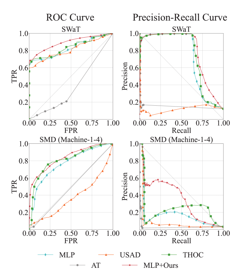
Figure 5: ROC curves (left) Precision-Recall curves (right) visualizations of baselines and MLP+Ours.

Analysis on ROC and Precision-Recall curves. Our method consistently outperforms previous approaches in terms of AUROC across all datasets except for SMD (M-1-4), and AUPRC across all datasets except for WADI and Creditcard. This indicates that previous off-the-shelf baselines are sensitive to threshold settings, which poses a challenge for robustness in real-world scenarios where finding an optimal threshold is difficult. Fig. 5 shows a visualization of the receiver operating curve (ROC curve) and precision-recall curve of our approach, along with baselines. Consistently, for both, our approach (red) improves the off-the-shelf classifier results (blue) significantly.

Results on AnoShift Benchmark

The AnoShift benchmark (Dragoi et al. 2022) offers a testbed for the robustness of anomaly detection algorithm under distribution shift problem. The dataset spans a decade, partitioned into a training set covering the period 2006-2010, and two distinct test sets denoted as NEAR (2011-2013) and FAR (2014-2015). Visualized in Fig. 6-(a), the data distribution progressively deviates from the train set as time progresses.

The principal objective of evaluation on the AnoShift benchmark is to investigate the effectiveness of our proposed algorithm against such distribution shifts. The evaluation entails three metrics—namely, Area Under the Receiver Operating Characteristic curve (AUROC), Area Under the Precision-Recall Curve with inliers as the positive class (AUPRC-in), and Area Under the Precision-Recall Curve with outliers as the positive class (AUPRC-out), following previous work (Dragoi et al. 2022). The performance of our method is compared to other deep-learning-based baselines, including SO-GAAL (Liu et al. 2020), deepSVDD (Ruff et al. 2018), LUNAR (Goodge et al. 2022), ICL (Shenkar and Wolf 2022), BERT (Devlin et al. 2019) for anomalies.

Table 2 demonstrates a significant improvement in performance when our method is integrated into an MLP-based autoencoder, as evidenced by an increase in AUROC of up to 0.216. Despite its simplicity, our approach markedly augments the baseline MLP performance, which previously showed inferior performance. This improvement is especially significant in FAR splits, which entail a severe distribution shift problem compared to NEAR splits. While our experiments focused on MLP, it’s worth noting that our module can be seamlessly added to other baselines.

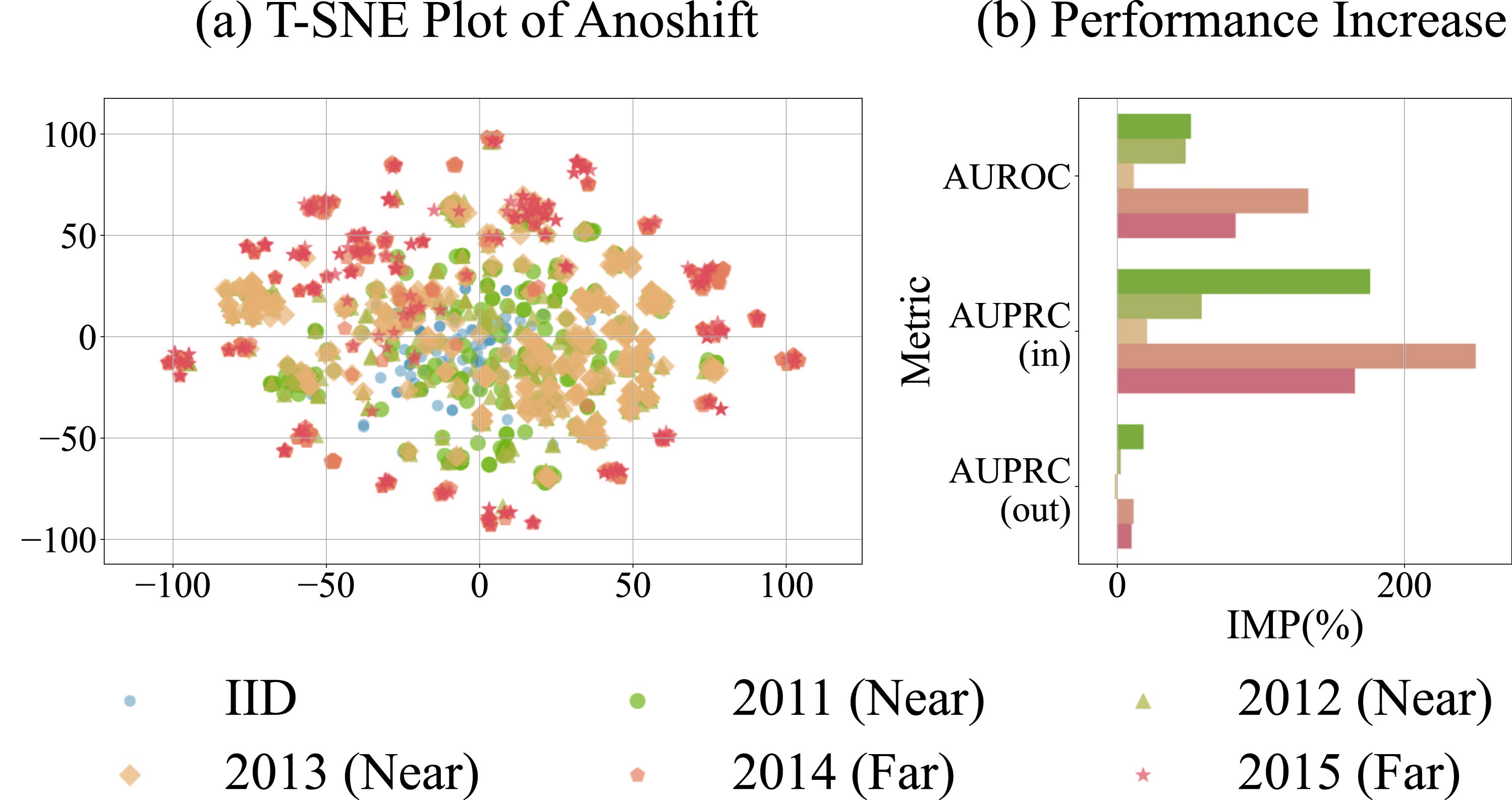
Figure 6: (a) T-SNE plot according to chronological distance and (b) performance increase with respect to three different evaluation metrics: AUROC, AUPRC-in and AUPRC-out.

Method	NEAR			FAR
	ROC	PRC (in)	PRC (out)	ROC	PRC (in)	PRC (out)
SO-GAAL†	0.545	0.435	0.877	0.493	0.107	0.927
deepSVDD†	0.870	0.717	0.942	0.345	0.100	0.823
LUNAR†	0.490	0.294	0.809	0.282	0.093	0.794
ICL†	0.523	0.273	0.819	0.225	0.088	0.775
BERT†	0.861	0.589	0.960	0.281	0.082	0.784
MLP†	0.441	0.262	0.730	0.200	0.085	0.757
MLP	0.441	0.207	0.776	0.208	0.085	0.758
MLP+Ours	0.639 (+0.194)	0.404 (+0.197)	0.841 (+0.065)	0.424 (+0.216)	0.259 (+0.173)	0.838 (+0.081)

Table 2: Performance on Anoshift benchmark. $\dagger$ denotes that metrics are reported from the results in the original paper. AUROC and AUPRC are denoted as ROC and PRC.

Ablation Study

Figure 7: F1 scores according to various thresholds.

DT	TTA	SWaT				SMD (M-2-1)				MSL (P-15)
		F1	F1-PA	AUROC	AUPRC	F1	F1-PA	AUROC	AUPRC	F1	F1-PA	AUROC	AUPRC
✗	✗	0.765	0.834	0.832	0.722	0.236	0.814	0.674	0.190	0.263	0.848	0.645	0.061
✓	✗	0.762	0.837	0.846	0.738	0.234	0.855	0.749	0.205	0.221	0.703	0.799	0.124
✗	✓	0.784	0.907	0.888	0.778	0.239	0.881	0.689	0.204	0.019	0.027	0.640	0.060
✓	✓	0.784	0.903	0.892	0.780	0.249	0.974	0.764	0.280	0.440	0.944	0.801	0.575

Table 3: Ablation study on our proposed method. DT and TTA indicate a detrend module and test-time adaptation, respectively.

As shown in Table 3, we perform the ablation study on our method to analyze the effectiveness of each component. MLP with detrend module and test-time adaptation with the model update is consistently showing better results, compared to the cases when used alone (MLP+DT, MLP+TTA) and none of them used (MLP). Here, DT and TTA denote a detrend module and test-time adaptation with model updates, respectively. Moreover, Fig. 7 also demonstrates that when the appropriate threshold is selected MLP model with our full method consistently outperforms these baselines, including the best performance of the off-the-shelf MLP model.

This behavior can be further described in Fig. 8-(a), illustrating those four options at once. (1) Our approach (red) shows better reconstruction compared to off-the-shelf MLP (blue). The off-the-shelf MLP model is constantly generating reconstruction errors even after the transition of an overall trend, which results in many false positive cases. (2) Also, the detrend module alone fails to detect anomalies, showing less sensitivity compared to our approach, although they share the same EMA parameter $\gamma$. This shows model update can contribute to such sensitivity of the anomaly detector, as it keeps updating with recent observations. (3) Without proper update of such trend estimate, test-time adaptation with model updates alone (green) can harm the robustness of the model, as it can be overfitted to sequence before trend shift, with a lack of ability to adapt to newly coming sequences.

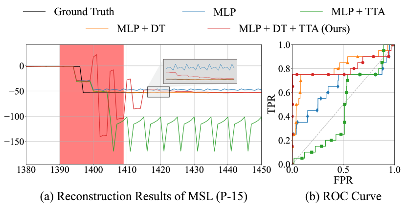
Figure 8: Ablation study on the proposed method using the MSL (P-15) dataset.

Discussion and Limitation

Threshold for Anomaly Detection. Existing unsupervised time-series anomaly detection studies (Audibert et al. 2020; Xu et al. 2022) have a major limitation in that they determine the threshold for normality by inferring the entire test data and selecting it based on the best performance. However, this approach is not practically feasible in real-world scenarios. Therefore, we report AUROC to evaluate overall performance and decide the threshold based on the training data statistics in our experiments. We posit that the performance of the anomaly detector could be further enhanced with an appropriate choice of threshold.

Inconsistent Labeling in Anomaly Detection. In the time-series anomaly detection task, the criteria of anomaly vary for each scenario, making it difficult to establish consistent labels. For this reason, distinguishing whether test samples with significant differences from the normal in train sets are abnormal or normal with distribution shifts is challenging. In our case, based on the assumption that there are more normal instances in test sets, we employ trend estimation and model predictions for test-time adaptation. To improve the adaptation performance, employing active learning (Ren et al. 2021) where human annotators provide labels for a subset of test data can be a valuable research direction.

Conclusion

In this work, we highlighted the distribution shift problem in unsupervised time-series anomaly detection. We have shown that the concept of normality may change over time. This can be a significant challenge for designing robust time-series anomaly detection frameworks, leading to many false positives, which harms the system’s consistency. To mitigate this issue, we propose a simple yet effective strategy of incorporating new normals into the model architecture, by following trend estimates along with test-time adaptation. Concretely, our method consistently outperforms standard baselines for real-world benchmarks with such problems.

Appendix A Detailed Dataset Description

Secure Water Treatment (SWaT) and WAter DIstribution (WADI) (Mathur and Tippenhauer 2016). The SWaT and WADI datasets encompass data collected from a testbed designed for cyber-physical systems involved in controlling water treatment processes. The SWaT dataset captures time-series data from 51 sensors and actuators deployed in industrial water treatment systems. This dataset spans a total of 11 days, consisting of 7 days of normal operation and 4 days for attack simulations. On the other hand, the WADI dataset focuses on a comprehensive system comprising water treatment, storage, and distribution networks. It includes 123 sensors deployed throughout the system. The dataset covers 16 days, encompassing 14 days of normal operations and 2 days of attack scenarios.

Server Machine Dataset (SMD) (Su et al. 2019). The SMD dataset, sourced from OmniAnomaly (Su et al. 2019), consists of a comprehensive collection of data spanning five weeks and encompassing 28 distinct machines. To facilitate model training and evaluation, each observation from a machine is partitioned into two segments. The first half of the sequence serves as the training data, while the latter half is designated as the test data. we specifically selected two datasets, namely SMD-machine-1-4 and SMD-machine-2-1, which are characterized by significant distributional shifts.

SMAP (Soil Moisture Active Passive) and Mars Science Laboratory (MSL). (Hundman et al. 2018) The SMAP/MSL dataset comprises expert-labeled data extracted from the reports of spacecraft monitoring systems. Specifically, the SMAP dataset consists of 55 telemetry channels, while the MSL dataset contains 27 telemetry channels. Within these datasets, there are 28 unique entities referred to as Incident Surprise Anomaly (ISA) Reports in SMAP and 19 in MSL. For our experimental analysis, we specifically selected two ISA entities, namely MSL (P-15) and SMAP (T-3), to investigate and evaluate their anomaly detection performance.

CreditCard. The CreditCard dataset consists of transaction logs of European cardholders spanning two days. For confidentiality reasons, the dataset only provides 28 principal component analysis (PCA) features, which have been anonymized, along with timestamp and transaction amount. The dataset is divided into two segments: the first half serves as the training dataset, while the latter half is designated as the test dataset.

Yahoo. The Yahoo dataset comprises both real (A1) and synthetic (A2, A3, A4) time-series data for anomaly detection. Our primary focus was on the real-world data (A1) characterized by distribution shifts. From this subset, we specifically selected two datasets, namely A1-R20 and A1-R55, which both are univariate time-series. In our experimental setup, the initial 400 timesteps were used as the training dataset, while the remaining timesteps were allocated for testing purposes.

Dataset	SWaT	WADI	SMD (M-1-4)	SMD (M-2-1)	MSL (P-15)	SMAP (T-3)	CreditCard	Yahoo (A1-R20)	Yahoo (A1-R55)
$|\mathcal{D}_{train}|$	496800	784571	23706	23693	3682	2876	142403	400	400
$|\mathcal{D}_{test}|$	449919	172803	23707	23694	2856	8579	142404	1022	1027
$F$	51	123	38	38	55	25	29	1	1
$\frac{|\mathcal{D}_{test}\cap\mathcal{D}_{\pi}|}{|\mathcal{D}_{test}|}$	12.1%	5.77%	0.0304%	0.0494	0.00700	0.0212	0.00157	0.0323	0.00487

Table 4: Dataset Descriptions. The number of observations in the training dataset and test dataset are denoted by $|\mathcal{D}_{train}|$ and $|\mathcal{D}_{test}|$ respectively. $F$ represents the number of features. Anomaly ratio during test-time is denoted as $\frac{|\mathcal{D}_{test}\cap\mathcal{D}_{\pi}|}{|\mathcal{D}_{test}|}$.

Appendix B Visualization Results of Datasets

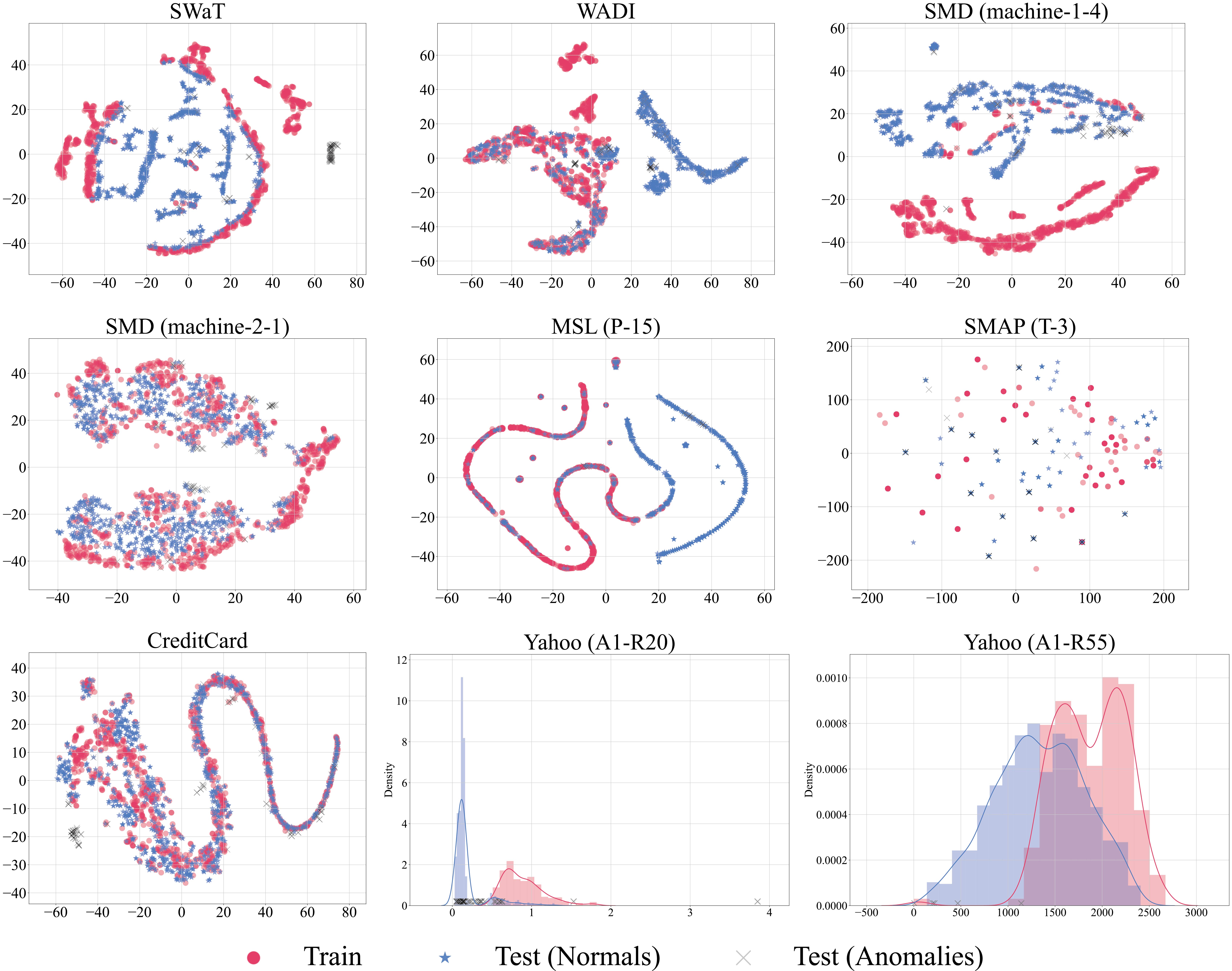
Figure 9: Visualization results of datasets. Red and blue each represent normal observations from the train and test datasets. Test-time anomalies are indicated by the symbol "X".

Figure 9 presents visualizations of the training and test dataset distributions for various benchmark datasets. T-SNE is used for visualization in all cases except for the Yahoo dataset, which contains univariate series.

It is worth noting that all datasets exhibit a "new normal problem", except for the CreditCard dataset. These visualizations highlight distinct behavior between the training (red) and test (blue) datasets. This discrepancy implies that off-the-shelf models are prone to generating numerous false positives, compromising the reliability of the monitoring system.

Specifically, our approach addresses this issue in datasets such as SWaT and SMD (M-2-1), where test-time anomalies are distinguishable from both training and test distributions. By adapting to test-time normals, our approach enhances detection performance. In contrast, datasets such as SMD (M-1-4), MSL(P-15), and Yahoo exhibit test-time anomalies that are visually indistinguishable from test-time normals.

These are cases of contextual anomalies, where values remain within the range of normal behavior, but anomalous events are defined by significant deviations from recent context. Nevertheless, even in these cases, fitting the model to normal behavior significantly reduces false positives.

In the case of the WADI dataset, a trade-off emerges between reducing false positives and potentially missing true positives. Our approach reduces false positives by 73% (from 102,824 to 75,076) while increasing true positives by 28% (from 8,122 to 3,248) in WADI, as detailed in Table 12. The significance of balancing this trade-off depends on the specific application, as a decrease in true positives or an increase in false positives may have varying consequences. Exploring strategies to achieve this balance depending on the application is a promising avenue for future research.

Appendix C Pseudocode for the proposed framework

In the method section, we suggest a simple algorithm for the model to adapt to new normals. In practice, our proposed methodology can be easily implemented by introducing an additional model update for the testing pipeline. Anomaly detector is denoted as $f_{\theta}$ where $\theta$ being model parameters, initially trained with $\mathcal{D}_{train}$. $\mathcal{D}_{test}$ with a stream of input length (or sliding window length) $w$ is assumed to arrive one after another. Hyperparameters include threshold $\tau$, test-time learning rate $\eta$, EMA update rate $\gamma$. Anomaly score of the stream is denoted as $\mathcal{A}(\mathcal{X}_{w,t})$.

Algorithm 1 Pseudocode for the proposed framework

Input: $f_{\theta}$, $\mathcal{D}_{test}$, $\tau$, $\eta$, $\gamma$.
Output: $\mathcal{A}(\mathcal{X}_{w,t})$

1:for $\mathcal{X}_{w,t}\ in\ \mathcal{D}_{test}$ do $\triangleright$ Stream input of length $w$

2:     $\mu_{t}\leftarrow\gamma\mu_{t-w}+(1-\gamma)\hat{\mu}$ $\triangleright$ Update trend estimate

3:     $\mathcal{A}(\mathcal{X}_{w,t})\leftarrow f_{\theta}(\mathcal{X}_{w,t},\tau)$ $\triangleright$ Anomaly Score of stream

4:     $\hat{\mathcal{Y}}_{w,t}\leftarrow\mathcal{A}(\mathcal{X}_{w,t})>\tau$ $\triangleright$ Mask that filters anomalies

5:     $\mathcal{L}(\cdot)\leftarrow(1-\hat{\mathcal{Y}}_{w,t})^{\top}\mathcal{L}(\mathcal{X}_{w,t})$ $\triangleright$ Filter normals

6:     $\theta\leftarrow\theta-\eta\nabla_{\theta}\mathcal{L}(\cdot)$ $\triangleright$ Update model parameters

7:end for

Appendix D Computational Cost Analysis

Measures	MLP	LSTM	USAD	THOC	AT
Running Time (ms)	0.402 ($\pm$0.030)	5.674 ($\pm$0.823)	0.732 ($\pm$0.009)	4.686 ($\pm$0.336)	4.407 ($\pm$0.112)
Total Flops	586740	84480	880110	1724360	4078068
Parameter Size (MB)	2.35	2.90	3.53	1.82	1.32
Forward/Backward Pass Size (MB)	0.01	0.03	0.02	0.11	0.33

Table 5: Computational Cost of Baselines.

Table 5 presents a comprehensive analysis of the computational costs associated with the baseline methods. In order to ensure a fair and accurate comparison, the following parameters were kept constant: window size ($w$) was set to 12, the number of features ($F$) was set to 55, the hidden dimension ($d$) was set to 128, and the batch size was set to 1. The computational cost was measured using a Titan Xp with CUDA version 11.1.

To evaluate the running time, the mean of 30 trials was calculated, along with their standard deviation, for a single batch. MLP demonstrated the lowest computational time among all the baselines, whereas LSTM had the least total flops for the operation with the longest computational time.

Appendix E Hyperparameter Settings

Table 6, 7, 8, 9, 10 present the default hyperparameter settings for the baseline models, along with the test-time hyperparameters ($\eta$, $\gamma$) for the MLP model. The default hyperparameters specified in the respective papers for Anomaly Transformer (Xu et al. 2022), USAD (Audibert et al. 2020) and THOC (Shen, Li, and Kwok 2020) are used for training. The official implementation of Anomaly Transformer  is employed, while the other models are re-implemented based on the architectural specifications provided in the papers.

In the context of test-time adaptation, a lower learning rate ($\eta$) and update speed ($\gamma$) are favored for SWaT, WADI, and CreditCard datasets, where longer sequences of instances are available in the test data. Conversely, for other datasets with shorter test datasets such as SMD, MSL, SMAP, and Yahoo, were updated relatively faster in both learning rate and trend estimate. In order to update with an identical scheme through time, SGD without momentum is used for test-time parameter update.

Datasets	SWaT	WADI	SMD (M-1-4)	SMD (M-2-1)	MSL (P-15)	SMAP (T-3)	CreditCard	Yahoo (A1-R20)	Yahoo (A1-R55)
$W$	12	12	5	5	5	5	12	5	5
$S_{train}$	12	12	5	5	5	5	12	1	1
$S_{test}$	12	12	5	5	5	5	12	5	5
$d$	128	128	16	16	16	16	128	2	2
$\gamma$	0.99999	0.99	0.4	0.99	0.6	0.8	0.999	0.9	0.1
$\eta$	0.005	0.001	0.1	0.05	0.1	1.0	0.01	0.005	0.005

Table 6: Hyperparameters for MLP model.

Datasets	SWaT	WADI	SMD (M-1-4)	SMD (M-2-1)	MSL (P-15)	SMAP (T-3)	CreditCard	Yahoo (A1-R20)	Yahoo (A1-R55)
$W$	12	12	5	5	5	5	12	5	5
$S_{train}$	12	12	5	5	5	5	12	5	5
$S_{test}$	12	12	5	5	5	5	12	5	5
$d$	128	128	128	128	128	128	128	128	128

Table 7: Hyperparameters for LSTM model.

Datasets	SWaT	WADI	SMD (M-1-4)	SMD (M-2-1)	MSL (P-15)	SMAP (T-3)	CreditCard	Yahoo (A1-R20)	Yahoo (A1-R55)
$W$	12	10	5	5	5	5	12	5	5
$S_{train}$	12	10	5	5	5	5	12	1	1
$S_{test}$	12	10	5	5	5	5	12	5	5
$d$	40	40	38	38	33	55	40	40	40

Table 8: Hyperparameters for USAD model.

Datasets	SWaT	WADI	SMD (M-1-4)	SMD (M-2-1)	MSL (P-15)	SMAP (T-3)	CreditCard	Yahoo (A1-R20)	Yahoo (A1-R55)
$W$	100	100	100	100	100	100	100	100	100
$S_{train}$	1	1	1	1	1	1	1	1	1
$S_{test}$	1	1	1	1	1	1	1	1	1
$d$	64	64	64	64	64	64	64	64	64

Table 9: Hyperparameters for THOC model.

Datasets	SWaT	WADI	SMD (M-1-4)	SMD (M-2-1)	MSL (P-15)	SMAP (T-3)	CreditCard	Yahoo (A1-R20)	Yahoo (A1-R55)
$W$	100	100	100	100	100	100	100	100	100
$S_{train}$	100	100	100	100	100	100	100	100	100
$S_{test}$	100	100	100	100	100	100	100	100	100
$r$	0.5	0.5	0.5	0.5	1.0	1.0	0.5	1.0	1.0

Table 10: Hyperparameters for Anomaly Transformer model.

Appendix F Detailed Experiment Results for Main Experiment and Ablation Study

Table 11: Detailed results for baseline models, except for MLP.

	Metrics	Thr	$\tau$	Acc	Prec	Rec	F1	AUROC	TN	FP	FN	TP	Acc+	Prec+	Rec+	F1+	TN+	FP+	FN+	TP+
LSTMEncDec	SWaT	$Q^{*}$	1.67E+07	0.827	0.377	0.646	0.476	0.749	337014	58321	19296	35288	0.848	0.434	0.819	0.567	337014	58321	9873	44711
		Q100	1.98E+08	0.880	0.963	0.010	0.021	0.749	395313	22	54011	573	0.962	0.999	0.685	0.813	395313	22	17203	37381
	WADI	$Q^{*}$	9.67E+14	0.951	0.997	0.150	0.260	0.531	162821	5	8484	1493	0.952	0.997	0.162	0.279	162821	5	8360	1617
		$Q^{*}$	9.67E+14	0.951	0.997	0.150	0.260	0.531	162821	5	8484	1493	0.952	0.997	0.162	0.279	162821	5	8360	1617
	SMD (M-1-4)	$Q^{*}$	4814.900	0.924	0.183	0.431	0.257	0.754	21604	1383	410	310	0.942	0.342	1	0.510	21604	1383	0	720
		$Q^{*}$	4814.900	0.924	0.183	0.431	0.257	0.754	21604	1383	410	310	0.942	0.342	1	0.510	21604	1383	0	720
	SMD (M-2-1)	$Q^{*}$	1308.600	0.912	0.248	0.386	0.302	0.745	21151	1373	718	452	0.942	0.460	1	0.630	21151	1373	0	1170
		Q100	812719.938	0.952	0.915	0.037	0.071	0.745	22520	4	1127	43	0.992	0.996	0.836	0.909	22520	4	192	978
	MSL (P-15)	$Q^{*}$	4.33E+07	0.952	0.040	0.250	0.068	0.599	2715	121	15	5	0.958	0.142	1	0.248	2715	121	0	20
		$Q^{*}$	4.33E+07	0.952	0.040	0.250	0.068	0.599	2715	121	15	5	0.958	0.142	1	0.248	2715	121	0	20
	SMAP (T-3)	$Q^{*}$	6450.760	0.977	0.263	0.055	0.091	0.525	8369	28	172	10	0.997	0.867	1	0.929	8369	28	0	182
		Q100	31647.510	0.978	0.222	0.011	0.021	0.525	8390	7	180	2	0.999	0.963	1	0.981	8390	7	0	182
	CreditCard	$Q^{*}$	10681.869	0.998	0.308	0.197	0.240	0.930	142082	99	179	44	0.998	0.336	0.224	0.269	142082	99	173	50
		$Q^{*}$	10681.869	0.998	0.308	0.197	0.240	0.930	142082	99	179	44	0.998	0.336	0.224	0.269	142082	99	173	50
	Yahoo (A1-R20)	$Q^{*}$	0.052	0.635	0.036	0.394	0.065	0.408	636	353	20	13	0.655	0.085	1	0.158	636	353	0	33
		Q99	0.186	0.795	0.027	0.152	0.046	0.408	808	181	28	5	0.816	0.126	0.788	0.217	808	181	7	26
	Yahoo (A1-R55)	$Q^{*}$	8.950	0.989	0.286	0.800	0.421	0.879	1012	10	1	4	0.989	0.286	0.800	0.421	1012	10	1	4
		$Q^{*}$	8.950	0.989	0.286	0.800	0.421	0.879	1012	10	1	4	0.989	0.286	0.800	0.421	1012	10	1	4
USAD	SWaT	$Q^{*}$	0.446	0.949	0.987	0.590	0.739	0.811	394910	425	22353	32231	0.959	0.988	0.668	0.797	394910	425	18106	36478
		$Q^{*}$	0.446	0.949	0.987	0.590	0.739	0.811	394910	425	22353	32231	0.959	0.988	0.668	0.797	394910	425	18106	36478
	WADI	$Q^{*}$	585.845	0.951	0.997	0.150	0.260	0.543	162821	5	8484	1493	0.952	0.997	0.162	0.279	162821	5	8360	1617
		$Q^{*}$	585.845	0.951	0.997	0.150	0.260	0.543	162821	5	8484	1493	0.952	0.997	0.162	0.279	162821	5	8360	1617
	SMD (M-1-4)	$Q^{*}$	20.129	0.969	0.397	0.037	0.069	0.374	22946	41	693	27	0.970	0.544	0.068	0.121	22946	41	671	49
		Q96	0.309	0.942	0.057	0.058	0.058	0.374	22295	692	678	42	0.945	0.128	0.142	0.135	22295	692	618	102
	SMD (M-2-1)	$Q^{*}$	0.075	0.925	0.269	0.303	0.285	0.744	21561	963	815	355	0.959	0.549	1	0.708	21561	963	0	1170
		Q98	0.113	0.951	0.519	0.115	0.189	0.744	22399	125	1035	135	0.991	0.897	0.928	0.912	22399	125	84	1086
	MSL (P-15)	$Q^{*}$	0.963	0.866	0.033	0.650	0.064	0.676	2460	376	7	13	0.868	0.051	1	0.096	2460	376	0	20
		$Q^{*}$	0.963	0.866	0.033	0.650	0.064	0.676	2460	376	7	13	0.868	0.051	1	0.096	2460	376	0	20
	SMAP (T-3)	$Q^{*}$	0.020	0.441	0.023	0.615	0.045	0.520	3672	4725	70	112	0.449	0.037	1	0.072	3672	4725	0	182
		Q99	0.121	0.976	0.071	0.011	0.019	0.520	8371	26	180	2	0.997	0.875	1	0.933	8371	26	0	182
	CreditCard	$Q^{*}$	0.017	0.998	0.292	0.359	0.322	0.931	141987	194	143	80	0.998	0.292	0.359	0.322	141987	194	143	80
		$Q^{*}$	0.017	0.998	0.292	0.359	0.322	0.931	141987	194	143	80	0.998	0.292	0.359	0.322	141987	194	143	80
	Yahoo (A1-R20)	$Q^{*}$	0.852	0.960	0.167	0.061	0.089	0.389	979	10	31	2	0.983	0.722	0.788	0.754	979	10	7	26
		$Q^{*}$	0.852	0.960	0.167	0.061	0.089	0.389	979	10	31	2	0.983	0.722	0.788	0.754	979	10	7	26
	Yahoo (A1-R55)	$Q^{*}$	0.462	0.996	1	0.200	0.333	0.875	1022	0	4	1	0.996	1	0.200	0.333	1022	0	4	1
		Q99	0.290	0.988	0.182	0.400	0.250	0.875	1013	9	3	2	0.989	0.250	0.600	0.353	1013	9	2	3
THOC	SWaT	$Q^{*}$	0.108	0.954	0.991	0.631	0.771	0.839	395008	327	20159	34425	0.966	0.992	0.726	0.838	395008	327	14974	39610
		$Q^{*}$	0.108	0.954	0.991	0.631	0.771	0.839	395008	327	20159	34425	0.966	0.992	0.726	0.838	395008	327	14974	39610
	WADI	$Q^{*}$	0.099	0.267	0.070	0.947	0.130	0.494	36621	126205	530	9447	0.270	0.073	1	0.137	36621	126205	0	9977
		Q97	0.100	0.440	0.061	0.600	0.110	0.494	70115	92711	3994	5983	0.463	0.097	1	0.177	70115	92711	0	9977
	SMD (M-1-4)	$Q^{*}$	0.101	0.927	0.207	0.490	0.291	0.812	21634	1353	367	353	0.940	0.323	0.897	0.475	21634	1353	74	646
		$Q^{*}$	0.101	0.927	0.207	0.490	0.291	0.812	21634	1353	367	353	0.940	0.323	0.897	0.475	21634	1353	74	646
	SMD (M-2-1)	$Q^{*}$	0.102	0.885	0.214	0.497	0.300	0.682	20391	2133	588	582	0.910	0.354	1	0.523	20391	2133	0	1170
		Q99	0.102	0.926	0.268	0.285	0.276	0.682	21613	911	837	333	0.962	0.562	1	0.720	21613	911	0	1170
	MSL (P-15)	$Q^{*}$	0.109	0.486	0.009	0.650	0.017	0.326	1374	1462	7	13	0.488	0.013	1	0.027	1374	1462	0	20
		$Q^{*}$	0.109	0.486	0.009	0.650	0.017	0.326	1374	1462	7	13	0.488	0.013	1	0.027	1374	1462	0	20
	SMAP (T-3)	$Q^{*}$	0.100	0.967	0.220	0.214	0.217	0.611	8259	138	143	39	0.984	0.569	1	0.725	8259	138	0	182
		Q97	0.102	0.972	0.191	0.099	0.130	0.611	8321	76	164	18	0.991	0.705	1	0.827	8321	76	0	182
	CreditCard	$Q^{*}$	0.104	0.998	0.192	0.184	0.188	0.864	142008	173	182	41	0.998	0.195	0.188	0.192	142008	173	181	42
		$Q^{*}$	0.104	0.998	0.192	0.184	0.188	0.864	142008	173	182	41	0.998	0.195	0.188	0.192	142008	173	181	42
	Yahoo (A1-R20)	$Q^{*}$	0.102	0.170	0.037	1	0.072	0.157	141	848	0	33	0.170	0.037	1	0.072	141	848	0	33
		$Q^{*}$	0.102	0.170	0.037	1	0.072	0.157	141	848	0	33	0.170	0.037	1	0.072	141	848	0	33
	Yahoo (A1-R55)	$Q^{*}$	0.107	0.884	0.025	0.600	0.048	0.847	905	117	2	3	0.884	0.025	0.600	0.048	905	117	2	3
		$Q^{*}$	0.107	0.884	0.025	0.600	0.048	0.847	905	117	2	3	0.884	0.025	0.600	0.048	905	117	2	3
Anomaly Transformer	SWaT	$Q^{*}$	0	0.121	0.121	1	0.216	0.382	0	395335	0	54584	0.121	0.121	1	0.216	0	395335	0	54584
		Q99	0.003	0.861	0.081	0.014	0.024	0.382	386657	8678	53818	766	0.981	0.863	1	0.926	386657	8678	0	54584
	WADI	$Q^{*}$	0.000	0.672	0.072	0.396	0.122	0.540	112241	50585	6026	3951	0.707	0.165	1	0.283	112241	50585	0	9977
		Q99	0.010	0.931	0.068	0.015	0.025	0.540	160763	2063	9827	150	0.988	0.829	1	0.906	160763	2063	0	9977
	SMD (M-1-4)	$Q^{*}$	0	0.030	0.030	1	0.059	0.508	0	22987	0	720	0.030	0.030	1	0.059	0	22987	0	720
		Q99	0.091	0.960	0.045	0.015	0.023	0.508	22752	235	709	11	0.985	0.720	0.838	0.774	22752	235	117	603
	SMD (M-2-1)	$Q^{*}$	0.00E+00	0.049	0.049	1	0.094	0.500	0	22524	0	1170	0.049	0.049	1	0.094	0	22524	0	1170
		Q99	0.170	0.942	0.059	0.012	0.020	0.500	22300	224	1156	14	0.985	0.823	0.893	0.857	22300	224	125	1045
	MSL (P-15)	$Q^{*}$	0.038	0.985	0.071	0.100	0.083	0.586	2810	26	18	2	0.991	0.435	1	0.606	2810	26	0	20
		Q100	33.389	0.988	0.067	0.050	0.057	0.586	2822	14	19	1	0.995	0.588	1	0.741	2822	14	0	20
	SMAP (T-3)	$Q^{*}$	0.00E+00	0.021	0.021	1	0.042	0.460	0	8397	0	182	0.021	0.021	1	0.042	0	8397	0	182
		Q99	0.003	0.969	0.022	0.011	0.015	0.460	8309	88	180	2	0.990	0.674	1	0.805	8309	88	0	182
	CreditCard	$Q^{*}$	3.800	0.998	0.155	0.067	0.094	0.549	142099	82	208	15	0.998	0.241	0.117	0.157	142099	82	197	26
		$Q^{*}$	3.800	0.998	0.155	0.067	0.094	0.549	142099	82	208	15	0.998	0.241	0.117	0.157	142099	82	197	26
	Yahoo (A1-R20)	$Q^{*}$	0	0.032	0.032	1	0.063	0.493	0	989	0	33	0.032	0.032	1	0.063	0	989	0	33
		Q98	0.000	0.929	0.024	0.030	0.027	0.493	948	41	32	1	0.934	0.146	0.212	0.173	948	41	26	7
	Yahoo (A1-R55)	$Q^{*}$	0.00E+00	0.005	0.005	1	0.010	0.483	0	1022	0	5	0.005	0.005	1	0.010	0	1022	0	5
		$Q^{*}$	0.00E+00	0.005	0.005	1	0.010	0.483	0	1022	0	5	0.005	0.005	1	0.010	0	1022	0	5

Table 12: Detailed results for ablation study.

	Metrics	Thr	$\tau$	Acc	Prec	Rec	F1	AUROC	TN	FP	FN	TP	Acc+	Prec+	Rec+	F1+	TN+	FP+	FN+	TP+
Off-the-shelf MLP	SWaT	$Q^{*}$	6.954	0.953	0.988	0.621	0.763	0.828	394908	427	20667	33917	0.965	0.989	0.721	0.834	394908	427	15218	39366
		Q99.98	4.723	0.949	0.918	0.633	0.750	0.828	392264	3071	20017	34567	0.965	0.931	0.765	0.840	392264	3071	12846	41738
	WADI	$Q^{*}$	0.141	0.394	0.073	0.814	0.134	0.499	60002	102824	1855	8122	0.405	0.088	1	0.163	60002	102824	0	9977
		Q99.6	1.208	0.446	0.057	0.551	0.103	0.499	71629	91197	4480	5497	0.472	0.099	1	0.180	71629	91197	0	9977
	SMD (M-1-4)	$Q^{*}$	0.822	0.931	0.189	0.383	0.253	0.793	21801	1186	444	276	0.950	0.378	1	0.548	21801	1186	0	720
		$Q^{*}$	0.822	0.931	0.189	0.383	0.253	0.793	21801	1186	444	276	0.950	0.378	1	0.548	21801	1186	0	720
	SMD (M-2-1)	$Q^{*}$	1.576	0.933	0.264	0.196	0.225	0.678	21885	639	941	229	0.973	0.647	1	0.785	21885	639	0	1170
		Q99	1.882	0.940	0.299	0.162	0.210	0.678	22080	444	981	189	0.981	0.725	1	0.841	22080	444	0	1170
	MSL (P-15)	$Q^{*}$	11.173	0.992	0.417	0.250	0.312	0.647	2829	7	15	5	0.998	0.741	1	0.851	2829	7	0	20
		$Q^{*}$	11.173	0.992	0.417	0.250	0.312	0.647	2829	7	15	5	0.998	0.741	1	0.851	2829	7	0	20
	SMAP (T-3)	$Q^{*}$	15.779	0.978	0.370	0.055	0.096	0.523	8380	17	172	10	0.998	0.915	1	0.955	8380	17	0	182
		Q100	46.906	0.978	0.286	0.011	0.021	0.523	8392	5	180	2	0.999	0.973	1	0.986	8392	5	0	182
	CreditCard	$Q^{*}$	22.099	0.997	0.150	0.143	0.146	0.946	141999	182	191	32	0.997	0.173	0.170	0.172	141999	182	185	38
		$Q^{*}$	22.099	0.997	0.150	0.143	0.146	0.946	141999	182	191	32	0.997	0.173	0.170	0.172	141999	182	185	38
	Yahoo (A1-R20)	$Q^{*}$	10.701	0.947	0.080	0.061	0.069	0.369	966	23	31	2	0.971	0.531	0.788	0.634	966	23	7	26
		$Q^{*}$	10.701	0.947	0.080	0.061	0.069	0.369	966	23	31	2	0.971	0.531	0.788	0.634	966	23	7	26
	Yahoo (A1-R55)	$Q^{*}$	18.927	0.989	0.250	0.600	0.353	0.921	1013	9	2	3	0.990	0.308	0.800	0.444	1013	9	1	4
		$Q^{*}$	18.927	0.989	0.250	0.600	0.353	0.921	1013	9	2	3	0.990	0.308	0.800	0.444	1013	9	1	4
MLP + DT	SWaT	Q99.98	4.723	0.953	0.980	0.627	0.765	0.843	394622	713	20348	34236	0.965	0.982	0.721	0.832	394622	713	15218	39366
		Q99.97	3.118	0.945	0.867	0.646	0.741	0.843	389935	5400	19315	35269	0.967	0.893	0.829	0.860	389935	5400	9353	45231
	WADI	$Q^{*}$	0.141	0.387	0.070	0.788	0.129	0.546	59045	103781	2116	7861	0.399	0.088	1	0.161	59045	103781	0	9977
		Q99.7	1.447	0.541	0.058	0.456	0.103	0.546	88922	73904	5426	4551	0.572	0.119	1	0.213	88922	73904	0	9977
	SMD (M-1-4)	Q98	0.248	0.964	0.418	0.483	0.448	0.838	22503	484	372	348	0.980	0.598	1	0.748	22503	484	0	720
		$Q^{*}$	0.822	0.972	0.568	0.260	0.357	0.838	22845	142	533	187	0.992	0.827	0.942	0.881	22845	142	42	678
	SMD (M-2-1)	Q98	1.136	0.927	0.237	0.219	0.228	0.751	21701	823	914	256	0.965	0.587	1	0.740	21701	823	0	1170
		Q99	1.882	0.944	0.345	0.156	0.215	0.751	22176	348	987	183	0.985	0.771	1	0.871	22176	348	0	1170
	MSL (P-15)	Q99	3.461	0.985	0.156	0.250	0.192	0.811	2809	27	15	5	0.991	0.426	1	0.597	2809	27	0	20
		$Q^{*}$	11.173	0.992	0.250	0.100	0.143	0.811	2830	6	18	2	0.998	0.769	1	0.870	2830	6	0	20
	SMAP (T-3)	Q95	0.007	0.945	0.097	0.192	0.129	0.581	8071	326	147	35	0.962	0.358	1	0.528	8071	326	0	182
		Q100	46.906	0.979	0.333	0.011	0.021	0.581	8393	4	180	2	1.000	0.978	1	0.989	8393	4	0	182
	CreditCard	Q99.93	20.458	0.997	0.139	0.143	0.141	0.939	141982	199	191	32	0.997	0.160	0.170	0.165	141982	199	185	38
		Q99.93	20.458	0.997	0.139	0.143	0.141	0.939	141982	199	191	32	0.997	0.160	0.170	0.165	141982	199	185	38
	Yahoo (A1-R20)	Q88	1.747	0.984	0.758	0.758	0.758	0.989	981	8	8	25	0.992	0.805	1	0.892	981	8	0	33
		Q90	2.041	0.980	0.783	0.545	0.643	0.989	984	5	15	18	0.995	0.868	1	0.930	984	5	0	33
	Yahoo (A1-R55)	Q94	2.447	0.998	1	0.600	0.750	0.953	1022	0	2	3	0.999	1	0.800	0.889	1022	0	1	4
		Q94	2.447	0.998	1	0.600	0.750	0.953	1022	0	2	3	0.999	1	0.800	0.889	1022	0	1	4
MLP + TTA	SWaT	Q99.6	0.537	0.956	0.936	0.680	0.788	0.888	392795	2540	17472	37112	0.974	0.947	0.836	0.888	392795	2540	8977	45607
		Q99.5	0.465	0.954	0.922	0.681	0.783	0.887	392212	3123	17418	37166	0.981	0.940	0.899	0.919	392212	3123	5515	49069
	WADI	Q92	0.090	0.390	0.074	0.832	0.136	0.492	59106	103720	1681	8296	0.400	0.088	1	0.161	59106	103720	0	9977
		Q99.5	1.052	0.446	0.057	0.550	0.103	0.496	71657	91169	4486	5491	0.472	0.099	1	0.180	71657	91169	0	9977
	SMD (M-1-4)	$Q^{*}$	0.822	0.916	0.148	0.374	0.212	0.767	21443	1544	451	269	0.935	0.318	1	0.483	21443	1544	0	720
		$Q^{*}$	0.822	0.916	0.148	0.374	0.212	0.767	21443	1544	451	269	0.935	0.318	1	0.483	21443	1544	0	720
	SMD (M-2-1)	$Q^{*}$	1.576	0.943	0.356	0.181	0.240	0.681	22140	384	958	212	0.984	0.753	1	0.859	22140	384	0	1170
		Q99	1.882	0.947	0.404	0.159	0.228	0.693	22250	274	984	186	0.988	0.810	1	0.895	22250	274	0	1170
	MSL (P-15)	Q93	0.395	0.461	0.010	0.750	0.019	0.571	1301	1535	5	15	0.463	0.013	1	0.025	1301	1535	0	20
		Q100	46.060	0.490	0.007	0.500	0.014	0.546	1390	1446	10	10	0.494	0.014	1	0.027	1390	1446	0	20
	SMAP (T-3)	$Q^{*}$	15.779	0.976	0.217	0.055	0.088	0.491	8361	36	172	10	0.996	0.835	1	0.910	8361	36	0	182
		$Q^{*}$	15.779	0.976	0.217	0.055	0.088	0.491	8361	36	172	10	0.996	0.835	1	0.910	8361	36	0	182
	CreditCard	Q99.93	20.458	0.997	0.148	0.161	0.154	0.947	141973	208	187	36	0.997	0.161	0.179	0.170	141973	208	183	40
		Q99.93	20.458	0.997	0.148	0.161	0.154	0.947	141973	208	187	36	0.997	0.161	0.179	0.170	141973	208	183	40
	Yahoo (A1-R20)	Q81	1.348	0.104	0.031	0.879	0.060	0.369	77	912	4	29	0.108	0.035	1	0.067	77	912	0	33
		Q100	13.274	0.969	1	0.030	0.059	0.598	989	0	32	1	0.970	1	0.061	0.114	989	0	31	2
	Yahoo (A1-R55)	$Q^{*}$	18.927	0.997	1	0.400	0.571	0.910	1022	0	3	2	0.997	1	0.400	0.571	1022	0	3	2
		$Q^{*}$	18.927	0.997	1	0.400	0.571	0.910	1022	0	3	2	0.997	1	0.400	0.571	1022	0	3	2
MLP + DT + TTA (Ours)	SWaT	Q99.56	0.626	0.955	0.954	0.664	0.783	0.889	393574	1761	18357	36227	0.978	0.963	0.848	0.902	393574	1761	8321	46263
		Q99.3	0.399	0.953	0.905	0.682	0.778	0.891	391419	3916	17358	37226	0.980	0.927	0.909	0.918	391419	3916	4975	49609
	WADI	Q99.9	2.753	0.800	0.105	0.326	0.159	0.629	135078	27748	6729	3248	0.822	0.202	0.705	0.314	135078	27748	2943	7034
		Q99.8	1.887	0.755	0.083	0.323	0.132	0.610	127243	35583	6754	3223	0.794	0.219	1	0.359	127243	35583	0	9977
	SMD (M-1-4)	Q97	0.215	0.968	0.469	0.490	0.480	0.845	22588	399	367	353	0.983	0.643	1	0.783	22588	399	0	720
		Q99	0.384	0.971	0.545	0.356	0.430	0.845	22773	214	464	256	0.991	0.771	1	0.871	22773	214	0	720
	SMD (M-2-1)	Q99.76	1.473	0.942	0.342	0.187	0.242	22102	422	951	219	0.982	0.735	1.0	0.847	22102	422	0	1170	0.703
		Q99	1.882	0.947	0.403	0.162	0.231	0.713	22242	282	980	190	0.988	0.806	1	0.892	22242	282	0	1170
	MSL (P-15)	Q99.9	28.991	0.996	0.909	0.500	0.645	0.809	2835	1	10	10	1.000	0.952	1	0.976	2835	1	0	20
		Q99.9	28.991	0.996	0.909	0.500	0.645	0.809	2835	1	10	10	1.000	0.952	1	0.976	2835	1	0	20
	SMAP (T-3)	Q96	0.078	0.958	0.153	0.220	0.180	0.605	8175	222	142	40	0.974	0.450	1.0	0.621	8175	222	0	182
		Q98	0.971	0.973	0.152	0.055	0.081	0.625	8341	56	172	10	0.993	0.765	1	0.867	8341	56	0	182
	CreditCard	Q99.93	20.458	0.997	0.154	0.170	0.162	0.946	141972	209	185	38	0.997	0.164	0.184	0.173	141972	209	182	41
		Q99.93	20.458	0.997	0.154	0.170	0.162	0.946	141972	209	185	38	0.997	0.164	0.184	0.173	141972	209	182	41
	Yahoo (A1-R20)	Q87	1.720	0.984	0.758	0.758	0.758	0.989	981	8	8	25	0.992	0.805	1	0.892	981	8	0	33
		Q90	2.041	0.980	0.783	0.545	0.643	0.989	984	5	15	18	0.995	0.868	1	0.930	984	5	0	33
	Yahoo (A1-R55)	Q95	2.762	0.998	1	0.600	0.750	0.954	1022	0	2	3	0.999	1	0.800	0.889	1022	0	1	4
		Q95	2.762	0.998	1	0.600	0.750	0.954	1022	0	2	3	0.999	1	0.800	0.889	1022	0	1	4

Table 11 and Table 12 provide detailed results for the main experiment and ablation study, respectively. In these tables, various metrics are reported to evaluate the performance of the models. The "Thr" column represents the threshold applied, while the symbol $\tau$ denotes the exact threshold value. Additionally, $Qp$ represents the $p$-th percentile of the train anomaly score, and $Q^{*}$ represents the threshold that maximizes the F1-score using the test anomaly scores and test labels, which is calculated using the ROC curve.

The available metrics include Accuracy (ACC), Precision (Prec), Recall (Rec), F1-score (F1), True Negatives (TN), False Positives (FP), False Negatives (FN), and True Positives (TP). Metrics reported with a "+" sign indicate that a point-adjust is applied. The first and second lines of each entry in the tables represent detailed results that maximize the F1-score and F1-PA (F1 with Point Adjust), respectively. It should be noted that the off-the-shelf baselines utilize $Q^{*}$ as the threshold to have maximum achievable performance for off-the-shelf baselines, while our approach sets the threshold using only the train anomaly scores.

Dataset	Metrics	MLP	LSTM	USAD	THOC	AT	Ours
SWaT	F1	0.765$\pm$0.002	0.401$\pm$0.060	0.557$\pm$0.174	0.776$\pm$0.012	0.218$\pm$0.003	0.784$\pm$0.003
	F1-PA	0.831$\pm$0.004	0.768$\pm$0.104	0.655$\pm$0.182	0.862$\pm$0.030	0.962$\pm$0.002	0.903$\pm$0.003
	AUROC	0.832$\pm$0.003	0.697$\pm$0.051	0.737$\pm$0.110	0.838$\pm$0.005	0.530$\pm$0.020	0.892$\pm$0.003
	AUPRC	0.722$\pm$0.004	0.248$\pm$0.046	0.457$\pm$0.228	0.744$\pm$0.008	0.195$\pm$0.033	0.780$\pm$0.002
WADI	F1	0.131$\pm$0.002	0.245$\pm$0.015	0.260$\pm$0.000	0.124$\pm$0.004	0.109$\pm$0.000	0.148$\pm$0.010
	F1-PA	0.175$\pm$0.010	0.279$\pm$0.000	0.279$\pm$0.000	0.153$\pm$0.013	0.915$\pm$0.003	0.346$\pm$0.022
	AUROC	0.485$\pm$0.005	0.525$\pm$0.004	0.530$\pm$0.029	0.484$\pm$0.008	0.501$\pm$0.002	0.624$\pm$0.004
	AUPRC	0.052$\pm$0.000	0.195$\pm$0.009	0.205$\pm$0.003	0.144$\pm$0.088	0.059$\pm$0.004	0.081$\pm$0.002
SMD (M-1-4)	F1	0.273$\pm$0.011	0.282$\pm$0.009	0.159$\pm$0.023	0.379$\pm$0.026	0.059$\pm$0.000	0.463$\pm$0.006
	F1-PA	0.544$\pm$0.026	0.500$\pm$0.016	0.296$\pm$0.043	0.521$\pm$0.023	0.799$\pm$0.020	0.874$\pm$0.006
	AUROC	0.805$\pm$0.007	0.818$\pm$0.029	0.673$\pm$0.044	0.869$\pm$0.032	0.479$\pm$0.011	0.845$\pm$0.002
	AUPRC	0.169$\pm$0.006	0.151$\pm$0.008	0.103$\pm$0.010	0.223$\pm$0.019	0.034$\pm$0.003	0.354$\pm$0.005
SMD (M-2-1)	F1	0.236$\pm$0.008	0.283$\pm$0.014	0.308$\pm$0.051	0.295$\pm$0.038	0.094$\pm$0.000	0.249$\pm$0.137
	F1-PA	0.814$\pm$0.023	0.910$\pm$0.010	0.922$\pm$0.002	0.705$\pm$0.038	0.866$\pm$0.017	0.974$\pm$0.004
	AUROC	0.674$\pm$0.015	0.727$\pm$0.007	0.738$\pm$0.040	0.668$\pm$0.031	0.498$\pm$0.004	0.764$\pm$0.022
	AUPRC	0.190$\pm$0.008	0.251$\pm$0.011	0.246$\pm$0.049	0.161$\pm$0.031	0.052$\pm$0.006	0.280$\pm$0.097
MSL (P-15)	F1	0.263$\pm$0.061	0.056$\pm$0.007	0.060$\pm$0.005	0.018$\pm$0.000	0.071$\pm$0.038	0.440$\pm$0.183
	F1-PA	0.848$\pm$0.028	0.351$\pm$0.146	0.097$\pm$0.013	0.027$\pm$0.000	0.437$\pm$0.357	0.944$\pm$0.018
	AUROC	0.645$\pm$0.006	0.617$\pm$0.011	0.661$\pm$0.010	0.332$\pm$0.004	0.568$\pm$0.088	0.801$\pm$0.011
	AUPRC	0.061$\pm$0.017	0.012$\pm$0.002	0.016$\pm$0.001	0.005$\pm$0.000	0.023$\pm$0.015	0.575$\pm$0.094
SMAP (T-3)	F1	0.095$\pm$0.002	0.091$\pm$0.007	0.044$\pm$0.001	0.154$\pm$0.089	0.042$\pm$0.000	0.218$\pm$0.032
	F1-PA	0.992$\pm$0.007	0.998$\pm$0.003	0.940$\pm$0.008	0.747$\pm$0.074	0.772$\pm$0.027	0.708$\pm$0.045
	AUROC	0.510$\pm$0.012	0.515$\pm$0.012	0.500$\pm$0.020	0.591$\pm$0.062	0.490$\pm$0.007	0.617$\pm$0.007
	AUPRC	0.044$\pm$0.003	0.050$\pm$0.011	0.031$\pm$0.001	0.049$\pm$0.029	0.017$\pm$0.003	0.111$\pm$0.015
Credit Card	F1	0.127$\pm$0.009	0.220$\pm$0.009	0.323$\pm$0.062	0.138$\pm$0.045	0.039$\pm$0.027	0.135$\pm$0.011
	F1-PA	0.145$\pm$0.015	0.234$\pm$0.019	0.323$\pm$0.062	0.148$\pm$0.045	0.056$\pm$0.041	0.151$\pm$0.009
	AUROC	0.943$\pm$0.003	0.930$\pm$0.005	0.887$\pm$0.048	0.770$\pm$0.027	0.548$\pm$0.033	0.943$\pm$0.002
	AUPRC	0.055$\pm$0.004	0.109$\pm$0.008	0.234$\pm$0.065	0.041$\pm$0.018	0.007$\pm$0.005	0.063$\pm$0.003
Yahoo (A1-R20)	F1	0.067$\pm$0.002	0.065$\pm$0.001	0.277$\pm$0.038	0.106$\pm$0.017	0.098$\pm$0.023	0.678$\pm$0.170
	F1-PA	0.259$\pm$0.243	0.426$\pm$0.216	0.695$\pm$0.086	0.106$\pm$0.017	0.185$\pm$0.042	0.895$\pm$0.051
	AUROC	0.367$\pm$0.001	0.394$\pm$0.012	0.668$\pm$0.031	0.198$\pm$0.022	0.525$\pm$0.017	0.971$\pm$0.036
	AUPRC	0.056$\pm$0.000	0.057$\pm$0.001	0.161$\pm$0.031	0.067$\pm$0.024	0.048$\pm$0.013	0.637$\pm$0.153
Yahoo (A1-R55)	F1	0.366$\pm$0.033	0.446$\pm$0.029	0.281$\pm$0.071	0.059$\pm$0.010	0.010$\pm$0.000	0.633$\pm$0.235
	F1-PA	0.424$\pm$0.070	0.446$\pm$0.029	0.320$\pm$0.093	0.059$\pm$0.010	0.010$\pm$0.000	0.744$\pm$0.290
	AUROC	0.916$\pm$0.006	0.877$\pm$0.044	0.867$\pm$0.022	0.875$\pm$0.028	0.478$\pm$0.004	0.958$\pm$0.011
	AUPRC	0.303$\pm$0.011	0.242$\pm$0.075	0.177$\pm$0.096	0.019$\pm$0.004	0.002$\pm$0.000	0.624$\pm$0.004

Table 13: Confidence interval report for the main experiment.

DT

TTA

SWaT

SMD (M-2-1)

MSL (P-15)

F1

F1-PA

AUROC

AUPRC

F1

F1-PA

AUROC

AUPRC

F1

F1-PA

AUROC

AUPRC

✗

✗

0.765 $\pm$0.002

0.834 $\pm$0.003

0.832 $\pm$0.003

0.722 $\pm$0.004

0.236 $\pm$0.008

0.814 $\pm$0.023

0.674 $\pm$0.015

0.190 $\pm$0.008

0.263 $\pm$0.061

0.848 $\pm$0.028

0.645 $\pm$0.006

0.061 $\pm$0.017

✓

✗

0.762 $\pm$0.006

0.837 $\pm$0.014

0.846 $\pm$0.005

0.738 $\pm$0.004

0.234 $\pm$0.007

0.855 $\pm$0.018

0.749 $\pm$0.011

0.205 $\pm$0.005

0.221 $\pm$0.019

0.703 $\pm$0.352

0.799 $\pm$0.008

0.124 $\pm$0.015

✗

✓

0.784 $\pm$0.001

0.907 $\pm$0.007

0.888 $\pm$0.003

0.778 $\pm$0.002

0.239 $\pm$0.006

0.881 $\pm$0.018

0.689 $\pm$0.007

0.204 $\pm$0.006

0.019 $\pm$0.000

0.027 $\pm$0.000

0.640 $\pm$0.036

0.060 $\pm$0.026

✓

✓

0.784 $\pm$0.003

0.903 $\pm$0.003

0.892 $\pm$0.003

0.780 $\pm$0.002

0.249 $\pm$0.137

0.974 $\pm$0.004

0.764 $\pm$0.022

0.280 $\pm$0.097

0.440 $\pm$0.183

0.944 $\pm$0.018

0.801 $\pm$0.011

0.575 $\pm$0.094

Table 14: Confidence interval report for the ablation study.

Appendix G Visualization of Anomaly Scores

Figure 10 presents the visualization results of anomaly scores, $\mathcal{A}(X_{t})$, for the SWaT test dataset. For MLP, the anomaly score is defined as the channel-wise mean of reconstruction errors for each timestep. For other baselines, anomaly scores are calculated following the definition of $\mathcal{A}(X_{t})$ for each model.

The upper five rows of figures display the anomaly scores obtained from off-the-shelf baselines (MLP, LSTM, USAD, THOC, AT), while the lower figure corresponds to MLP with our adaptation strategy. The black horizontal line represents the threshold ($\tau$) applied, the red shade indicates the ground truth anomaly labels, and the gray shade represents the models’ predictions of anomalies. To facilitate visualization, all anomaly scores, including thresholds, have been scaled to the range of 0 to 1.

It is evident from the visualization that all off-the-shelf baselines exhibit gradually increasing anomaly scores. This indicates that these models have failed to adapt to the changing trend and dynamics observed during the test phase. In contrast, our proposed approach demonstrates robustness in the face of such shifts, which serves as the primary driver behind the observed performance improvements.

Figure 10: Visualization of anomaly scores for various baselines and our method. The black horizontal line represents the threshold ($\tau$) applied, the red shade indicates the ground truth anomaly labels, and the gray shade represents the models’ predictions of anomalies.

References

- Abdulaal, Liu, and Lancewicki (2021) Abdulaal, A.; Liu, Z.; and Lancewicki, T. 2021. Practical Approach to Asynchronous Multivariate Time Series Anomaly Detection and Localization. In Proc. the ACM SIGKDD International Conference on Knowledge Discovery and Data Mining (KDD).
- Audibert et al. (2020) Audibert, J.; Michiardi, P.; Guyard, F.; Marti, S.; and Zuluaga, M. A. 2020. USAD: UnSupervised Anomaly Detection on Multivariate Time Series. In Proc. the ACM SIGKDD International Conference on Knowledge Discovery and Data Mining (KDD).
- Breunig et al. (2000) Breunig, M. M.; Kriegel, H.; Ng, R. T.; and Sander, J. 2000. LOF: Identifying Density-Based Local Outliers. In Proceedings of the 2000 ACM SIGMOD International Conference on Management of Data, May 16-18, 2000, Dallas, Texas, USA.
- Cao, Zhu, and Pang (2023) Cao, T.; Zhu, J.; and Pang, G. 2023. Anomaly Detection under Distribution Shift. CoRR, abs/2303.13845.
- Choi et al. (2022) Choi, S.; Yang, S.; Choi, S.; and Yun, S. 2022. Improving test-time adaptation via shift-agnostic weight regularization and nearest source prototypes. In Proc. of the European Conference on Computer Vision (ECCV), 440–458. Springer.
- Devlin et al. (2019) Devlin, J.; Chang, M.; Lee, K.; and Toutanova, K. 2019. BERT: Pre-training of Deep Bidirectional Transformers for Language Understanding. In Burstein, J.; Doran, C.; and Solorio, T., eds., Proc. of The Annual Conference of the North American Chapter of the Association for Computational Linguistics (NAACL).
- Dragoi et al. (2022) Dragoi, M.; Burceanu, E.; Haller, E.; Manolache, A.; and Brad, F. 2022. AnoShift: A Distribution Shift Benchmark for Unsupervised Anomaly Detection. In NeurIPS.
- Ganin et al. (2016) Ganin, Y.; Ustinova, E.; Ajakan, H.; Germain, P.; Larochelle, H.; Laviolette, F.; Marchand, M.; and Lempitsky, V. 2016. Domain-adversarial training of neural networks. The journal of machine learning research, 17(1): 2096–2030.
- Geiger et al. (2020) Geiger, A.; Liu, D.; Alnegheimish, S.; Cuesta-Infante, A.; and Veeramachaneni, K. 2020. TadGAN: Time Series Anomaly Detection Using Generative Adversarial Networks. In 2020 IEEE International Conference on Big Data (IEEE BigData 2020), Atlanta, GA, USA, December 10-13, 2020, 33–43. IEEE.
- Goodge et al. (2022) Goodge, A.; Hooi, B.; Ng, S.; and Ng, W. S. 2022. LUNAR: Unifying Local Outlier Detection Methods via Graph Neural Networks. In Proc. the AAAI Conference on Artificial Intelligence (AAAI).
- Gulrajani and Lopez-Paz (2021) Gulrajani, I.; and Lopez-Paz, D. 2021. In Search of Lost Domain Generalization. In Proc. the International Conference on Learning Representations (ICLR).
- Han et al. (2021) Han, C.; Rundo, L.; Murao, K.; Noguchi, T.; Shimahara, Y.; Milacski, Z. Á.; Koshino, S.; Sala, E.; Nakayama, H.; and Satoh, S. 2021. MADGAN: unsupervised medical anomaly detection GAN using multiple adjacent brain MRI slice reconstruction. BMC Bioinform., 22-S(2): 31.
- Hundman et al. (2018) Hundman, K.; Constantinou, V.; Laporte, C.; Colwell, I.; and Söderström, T. 2018. Detecting Spacecraft Anomalies Using LSTMs and Nonparametric Dynamic Thresholding. In Proc. the ACM SIGKDD International Conference on Knowledge Discovery and Data Mining (KDD).
- Kim et al. (2022a) Kim, S.; Choi, K.; Choi, H.; Lee, B.; and Yoon, S. 2022a. Towards a Rigorous Evaluation of Time-Series Anomaly Detection. In Proc. the AAAI Conference on Artificial Intelligence (AAAI).
- Kim et al. (2022b) Kim, T.; Kim, J.; Tae, Y.; Park, C.; Choi, J.; and Choo, J. 2022b. Reversible Instance Normalization for Accurate Time-Series Forecasting against Distribution Shift. In Proc. the International Conference on Learning Representations (ICLR).
- Lai et al. (2021) Lai, K.; Zha, D.; Xu, J.; Zhao, Y.; Wang, G.; and Hu, X. 2021. Revisiting Time Series Outlier Detection: Definitions and Benchmarks. In Proc. the Advances in Neural Information Processing Systems (NeurIPS).
- Liang, Hu, and Feng (2020) Liang, J.; Hu, D.; and Feng, J. 2020. Do we really need to access the source data? source hypothesis transfer for unsupervised domain adaptation. In International Conference on Machine Learning, 6028–6039. PMLR.
- Liu, Liu, and Peng (2016) Liu, L.; Liu, D.; and Peng, Y. 2016. Detection and identification of sensor anomaly for aerospace applications. In 2016 Annual Reliability and Maintainability Symposium (RAMS), 1–6. IEEE.
- Liu et al. (2020) Liu, Y.; Li, Z.; Zhou, C.; Jiang, Y.; Sun, J.; Wang, M.; and He, X. 2020. Generative Adversarial Active Learning for Unsupervised Outlier Detection. IEEE Trans. Knowl. Data Eng., 32(8): 1517–1528.
- Liu et al. (2022) Liu, Y.; Wu, H.; Wang, J.; and Long, M. 2022. Non-stationary Transformers: Exploring the Stationarity in Time Series Forecasting. In NeurIPS.
- Malhotra et al. (2016) Malhotra, P.; Ramakrishnan, A.; Anand, G.; Vig, L.; Agarwal, P.; and Shroff, G. 2016. LSTM-based Encoder-Decoder for Multi-sensor Anomaly Detection. CoRR, abs/1607.00148.
- Mathur and Tippenhauer (2016) Mathur, A. P.; and Tippenhauer, N. O. 2016. SWaT: a water treatment testbed for research and training on ICS security. In 2016 International Workshop on Cyber-physical Systems for Smart Water Networks, CySWater@CPSWeek 2016, Vienna, Austria, April 11, 2016.
- Muth (1960) Muth, J. F. 1960. Optimal properties of exponentially weighted forecasts. Journal of the american statistical association, 55(290): 299–306.
- Niu et al. (2022) Niu, S.; Wu, J.; Zhang, Y.; Chen, Y.; Zheng, S.; Zhao, P.; and Tan, M. 2022. Efficient test-time model adaptation without forgetting. In Proc. the International Conference on Machine Learning (ICML), 16888–16905. PMLR.
- Pang et al. (2022) Pang, G.; Shen, C.; Cao, L.; and van den Hengel, A. 2022. Deep Learning for Anomaly Detection: A Review. ACM Comput. Surv., 54(2): 38:1–38:38.
- Park, Hoshi, and Kemp (2018) Park, D.; Hoshi, Y.; and Kemp, C. C. 2018. A Multimodal Anomaly Detector for Robot-Assisted Feeding Using an LSTM-Based Variational Autoencoder. IEEE Robotics Autom. Lett.
- Pena, de Assis, and Jr. (2013) Pena, E. H. M.; de Assis, M. V. O.; and Jr., M. L. P. 2013. Anomaly Detection Using Forecasting Methods ARIMA and HWDS. In 32nd International Conference of the Chilean Computer Science Society, SCCC 2013, Temuco, Cautin, Chile, November 11-15, 2013, 63–66. IEEE Computer Society.
- Quinonero-Candela et al. (2008) Quinonero-Candela, J.; Sugiyama, M.; Schwaighofer, A.; and Lawrence, N. D. 2008. Dataset shift in machine learning. Mit Press.
- Rassam, Maarof, and Zainal (2018) Rassam, M. A.; Maarof, M. A.; and Zainal, A. 2018. A distributed anomaly detection model for wireless sensor networks based on the one-class principal component classifier. Int. J. Sens. Networks, 27(3): 200–214.
- Ren et al. (2021) Ren, P.; Xiao, Y.; Chang, X.; Huang, P.-Y.; Li, Z.; Gupta, B. B.; Chen, X.; and Wang, X. 2021. A survey of deep active learning. ACM computing surveys (CSUR), 54(9): 1–40.
- Ruff et al. (2018) Ruff, L.; Görnitz, N.; Deecke, L.; Siddiqui, S. A.; Vandermeulen, R. A.; Binder, A.; Müller, E.; and Kloft, M. 2018. Deep One-Class Classification. In Proc. the International Conference on Machine Learning (ICML).
- Ruff et al. (2021) Ruff, L.; Kauffmann, J. R.; Vandermeulen, R. A.; Montavon, G.; Samek, W.; Kloft, M.; Dietterich, T. G.; and Müller, K. 2021. A Unifying Review of Deep and Shallow Anomaly Detection. Proc. IEEE, 109(5): 756–795.
- Saito and Rehmsmeier (2015) Saito, T.; and Rehmsmeier, M. 2015. The precision-recall plot is more informative than the ROC plot when evaluating binary classifiers on imbalanced datasets. PloS one, 10(3): e0118432.
- Sankararaman et al. (2022) Sankararaman, A.; Narayanaswamy, B.; Singh, V. Y.; and Song, Z. 2022. FITNESS: (Fine Tune on New and Similar Samples) to detect anomalies in streams with drift and outliers. In Proc. the International Conference on Machine Learning (ICML).
- Saurav et al. (2018) Saurav, S.; Malhotra, P.; TV, V.; Gugulothu, N.; Vig, L.; Agarwal, P.; and Shroff, G. 2018. Online anomaly detection with concept drift adaptation using recurrent neural networks. In Proceedings of the ACM India Joint International Conference on Data Science and Management of Data, COMAD/CODS 2018, Goa, India, January 11-13, 2018.
- Schlegl et al. (2017) Schlegl, T.; Seeböck, P.; Waldstein, S. M.; Schmidt-Erfurth, U.; and Langs, G. 2017. Unsupervised Anomaly Detection with Generative Adversarial Networks to Guide Marker Discovery. In Information Processing in Medical Imaging - 25th International Conference, IPMI 2017, Boone, NC, USA, June 25-30, 2017, Proceedings, volume 10265 of Lecture Notes in Computer Science, 146–157. Springer.
- Schölkopf et al. (1999) Schölkopf, B.; Williamson, R. C.; Smola, A. J.; Shawe-Taylor, J.; and Platt, J. C. 1999. Support Vector Method for Novelty Detection. In Solla, S. A.; Leen, T. K.; and Müller, K., eds., Proc. the Advances in Neural Information Processing Systems (NeurIPS).
- Shen, Li, and Kwok (2020) Shen, L.; Li, Z.; and Kwok, J. T. 2020. Timeseries Anomaly Detection using Temporal Hierarchical One-Class Network. In Proc. the Advances in Neural Information Processing Systems (NeurIPS).
- Shenkar and Wolf (2022) Shenkar, T.; and Wolf, L. 2022. Anomaly Detection for Tabular Data with Internal Contrastive Learning. In Proc. the International Conference on Learning Representations (ICLR).
- Shin et al. (2020) Shin, Y.; Lee, S.; Tariq, S.; Lee, M. S.; Jung, O.; Chung, D.; and Woo, S. S. 2020. ITAD: Integrative Tensor-based Anomaly Detection System for Reducing False Positives of Satellite Systems. In Proc. the ACM Conference on Information and Knowledge Management (CIKM).
- Shumway and Stoffer (2017) Shumway, R. H.; and Stoffer, D. S. 2017. Time series analysis and its applications: With R examples. Springer.
- Sørbø and Ruocco (2023) Sørbø, S.; and Ruocco, M. 2023. Navigating the Metric Maze: A Taxonomy of Evaluation Metrics for Anomaly Detection in Time Series. CoRR, abs/2303.01272.
- Su et al. (2019) Su, Y.; Zhao, Y.; Niu, C.; Liu, R.; Sun, W.; and Pei, D. 2019. Robust Anomaly Detection for Multivariate Time Series through Stochastic Recurrent Neural Network. In Proc. the ACM SIGKDD International Conference on Knowledge Discovery and Data Mining (KDD).
- Sun et al. (2020) Sun, Y.; Wang, X.; Liu, Z.; Miller, J.; Efros, A. A.; and Hardt, M. 2020. Test-Time Training with Self-Supervision for Generalization under Distribution Shifts. In Proc. the International Conference on Machine Learning (ICML).
- Tax and Duin (1999) Tax, D. M. J.; and Duin, R. P. W. 1999. Data domain description using support vectors. In 7th European Symposium on Artificial Neural Networks, ESANN 1999, Bruges, Belgium, April 21-23, 1999, Proceedings.
- Wang et al. (2021) Wang, D.; Shelhamer, E.; Liu, S.; Olshausen, B. A.; and Darrell, T. 2021. Tent: Fully Test-Time Adaptation by Entropy Minimization. In Proc. the International Conference on Learning Representations (ICLR).
- Wang, Kuang, and Duan (2015) Wang, J.; Kuang, Q.; and Duan, S. 2015. A new online anomaly learning and detection for large-scale service of Internet of Thing. Pers. Ubiquitous Comput., 19(7): 1021–1031.
- Wang et al. (2022) Wang, Q.; Fink, O.; Gool, L. V.; and Dai, D. 2022. Continual Test-Time Domain Adaptation. In Proc. of the IEEE conference on computer vision and pattern recognition (CVPR).
- Xu et al. (2018) Xu, H.; Chen, W.; Zhao, N.; Li, Z.; Bu, J.; Li, Z.; Liu, Y.; Zhao, Y.; Pei, D.; Feng, Y.; Chen, J.; Wang, Z.; and Qiao, H. 2018. Unsupervised Anomaly Detection via Variational Auto-Encoder for Seasonal KPIs in Web Applications. In Proc. the International Conference on World Wide Web (WWW).
- Xu et al. (2022) Xu, J.; Wu, H.; Wang, J.; and Long, M. 2022. Anomaly Transformer: Time Series Anomaly Detection with Association Discrepancy. In Proc. the International Conference on Learning Representations (ICLR).
- Yoo, Chung, and Kwak (2022) Yoo, J.; Chung, I.; and Kwak, N. 2022. Unsupervised Domain Adaptation for One-Stage Object Detector Using Offsets to Bounding Box. In Proc. of the European Conference on Computer Vision (ECCV), 691–708. Springer.
- Zinkevich (2003) Zinkevich, M. 2003. Online Convex Programming and Generalized Infinitesimal Gradient Ascent. In Proc. the International Conference on Machine Learning (ICML).
- Zong et al. (2018) Zong, B.; Song, Q.; Min, M. R.; Cheng, W.; Lumezanu, C.; Cho, D.; and Chen, H. 2018. Deep Autoencoding Gaussian Mixture Model for Unsupervised Anomaly Detection. In Proc. the International Conference on Learning Representations (ICLR).
- Zou et al. (2018) Zou, Y.; Yu, Z.; Kumar, B.; and Wang, J. 2018. Unsupervised domain adaptation for semantic segmentation via class-balanced self-training. In Proc. of the European Conference on Computer Vision (ECCV), 289–305.