Supplement - ’Automatic Parameter Selection for Non-Redundant Clustering’

1 Symbols

We use the following symbols in our paper as well as in the supplement:

Table 1: Description of the used symbols.

Symbol	Interpretation
$N\in\mathbb{N}$	Number of objects
$d\in\mathbb{N}$	Dimensionality of the feature space
$J\in\mathbb{N}$	Number of subspaces
$V\in\mathbb{R}^{d\times d}$	Orthogonal (rotation) matrix
$\delta\in\mathbb{R}$	The precision of the encoding
$I_{m_{j}}\in\mathbb{N}^{m_{j}\times m_{j}}$	$m_{j}\times m_{j}$ identity matrix
$X\subseteq\mathbb{R}^{d}$	Set of all objects
$k_{j}\in\mathbb{N}$	Number of clusters in subspace $j$
$m_{j}\in\mathbb{N}$	Dimensionality of subspace $j$
$P_{j}\in\mathbb{N}^{d\times m_{j}}$	Projection matrix of subspace $j$
$p_{j}\in\mathbb{N}$	Number of distribution-specific parameters in subspace $j$
$X_{j}\subseteq\mathbb{R}^{m_{j}}$	X projected to subspace $j$
$O_{j}\subseteq X_{j}$	Set of outliers in subspace $j$
$\mu_{j,i}\in\mathbb{R}^{m_{j}}$	Center of cluster $i$ in subspace $j$
$\Sigma_{j,i}\in\mathbb{R}^{m_{j}\times m_{j}}$	Covariance matrix of cluster $i$ in subspace $j$
$C_{j,i}\subseteq X_{j}$	Objects of cluster $i$ in subspace $j$
$J_{p}\in\mathbb{N}$	Number of predicted subspaces
$J{gt}\in\mathbb{N}$	Number of true subspaces
$R^{p}\in\mathbb{N}^{N\times J_{p}}$	Prediction labels matrix
$R^{gt}\in\mathbb{N}^{N\times J_{gt}}$	Ground truth labels matrix

2 Encoding the Constant Values

At this point, we would like to give a brief intuition on how the constant components of the encoding strategy we present in the paper could be handled.

The number of objects $N$ and dimensionality $d$ can again be encoded using the natural prior for integers. Therefore, we need $L^{0}(N)+L^{0}(d)$ bits to encode these values.

In general real values $r$ can be encoded by separately encoding the integer part $\lfloor r\rfloor$ and the decimal places [5]. Here, the precision $\delta$ is required for the decimal places. Hence, the following applies:

$$L(r)=L^{0}(\lfloor r\rfloor)-\log_{2}(\delta).$$

This can be used to encode the $d+1$ values needed to define the hypercube. It can also be used to encode $V$. Since all the column vectors of $V$ are orthonormal, they all have a length of $1$. Therefore, all values of a column are less than or equal to $1$ and we can consequently ignore $L^{0}(\lfloor r\rfloor)$. Moreover, since the orientation is indifferent, the last entry can be calculated using the first $d-1$ entries. Thereby each column loses one degree of freedom. Furthermore, the orthogonal property means that each following column loses an additional degree of freedom. Therefore, we can encode the first column using $-\log_{2}(\delta)(d-1)$ bits, the second with $-\log_{2}(\delta)(d-2)$ bits, and so forth. All in all, the code length of $V$ is $-\log_{2}(\delta)\frac{d(d-1)}{2}$.

From these encodings, it is very easy to see that the values are actually constants that are independent of a particular clustering result.

3 Search Space Restrictions

In this section, we would like to justify our restrictions on the search space with an example.

In the paper, we say that we restrict the number of clusters in case of a cluster space split as follows:

$$\text{max}(k_{\text{split}_{1}},k_{\text{split}_{2}})\leq k_{\text{original}}\leq k_{\text{split}_{1}}\cdot k_{\text{split}_{2}}.$$

Also, we restrict the number of clusters for a cluster space merge with the inverted rule.

$$\text{max}(k_{\text{original}_{1}},k_{\text{original}_{2}})\leq k_{\text{merge}}\leq k_{\text{original}_{1}}\cdot k_{\text{original}_{2}}$$

(a) Subspace with $4$ clusters.

(b) Subspace with $3$ clusters.

Figure 1: Histograms of two $1$-dimensional subspaces.

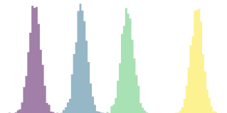
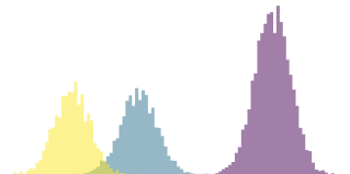
To better understand these rules, assume that we have the $1$-dimensional subspaces shown in Figure 1 with $4$ and $3$ clusters, respectively. If we want to merge these subspaces, we will always get at least 4 clusters, since 4 clusters are already contained in the first subspace. Moreover, there are a maximum of $12$ cluster combinations that can occur. Both extreme situations are illustrated in Figure 2.

(a) Combination with the minimum number of $4$ clusters.

(b) Combination with the maximum number of $12$ clusters.

Figure 2: Two possible combinations of the two subspaces from Figure 1.

With a cluster space split, essentially the same applies, but in reverse. Here, no subspace may be created that already has more than the original number of clusters. Furthermore, $k_{\text{split}_{1}}\cdot k_{\text{split}_{2}}$ must be greater than or equal to the original number of clusters. If one of these two rules is not met, subspaces would be created that do not fit the structure of the original subspace.

These rules can also be applied to higher dimensional subspaces.

4 Pseudo-code

1 Function main(dataset $X$)

2       $V$ = initialize randomly

3       $R_{\text{best}}$ = Initial result (single noise space)

4       // Sort by MDL costs, add noise space last

5       sortedSpaces = sortSubspaces($R_{\text{best}}$)

6       for $j\in sortedSpaces$ do

7             $X_{j}=\{xVP_{j}|x\in X\}$

8             if $j$ is cluster space then

9                   // Split space into two cluster spaces

10                   $j_{s_{1}},j_{s_{2}}$ = clusterSpaceSplit($X_{j}$, $k_{j}$)

11                  

12            else if $j$ is noise space then

13                   // Split space into cluster and noise space

14                   $j_{s_{1}},j_{s_{2}}$ = noiseSpaceSplit($X_{j}$)

15                  

16            // Check MDL costs

17             if cost($j_{s_{1}}$) + cost($j_{s_{2}}$) $<$ cost($j$) then

18                   // Join parameters for full-space execution

19                   $V_{\text{tmp}},P_{\text{tmp}},\mu_{\text{tmp}}$ = joinParams($R_{\text{best}},V,j_{s_{1}},j_{s_{2}}$)

20                   $R_{\text{tmp}}$, $V_{\text{tmp}}$ = fullSpace($X,V_{\text{tmp}},P_{\text{tmp}},\mu_{\text{tmp}}$)

21                   // Check full-space MDL costs

22                   if cost($R_{\text{tmp}}$) $<$ cost($R_{\text{best}}$) then

23                         $R_{\text{best}}$ $=$ $R_{\text{tmp}}$; $V=V_{\text{tmp}}$

24                         go to line 1

25                        

26                  

27            

28      $R_{\text{best}},V$ = merging($R_{\text{best}},V$)

29       if merging was successful then

30             go to line 1

31      return $R_{\text{best}}$

32

33 Function merging($R_{\text{best}},V$)

34      

35      for each pair ($j_{1}$, $j_{2}$) of cluster spaces  do

36             $X_{j_{1},j_{2}}=\{xVP_{j_{1},j_{2}}|x\in X\}$

37             $j_{m}$ = clusterSpaceMerge($X_{j_{1},j_{2}}$, $k_{j_{1}}$, $k_{j_{2}}$)

38             // Check MDL costs

39             if cost($j_{m}$) $<$ cost($j_{1}$) + cost($j_{2}$) then

40                   // Join parameters for the full-space execution

41                   $V_{\text{tmp}},P_{\text{tmp}},\mu_{\text{tmp}}$ = joinParams($R_{\text{best}},V,j_{m}$)

42                   $R_{\text{tmp}},V_{\text{tmp}}$ = fullSpace($X,V_{\text{tmp}},P_{\text{tmp}},\mu_{\text{tmp}}$)

43                   // Check full-space MDL costs

44                   if cost($R_{\text{tmp}}$) $<$ cost($R_{\text{best}}$) then

45                         $R_{\text{best}}=R_{\text{tmp}}$; $V=V_{\text{tmp}}$

46                        

47                  

48            

49      if better result found then

50             go to line 1

51      return $R_{\text{best}},V$

Algorithm 1 Parameter search algorithm.

In order to determine the number of subspaces and clusters within subspaces for non-redundant clustering, the following steps are executed:

• Noise Space Split

• Cluster Space Split

• Cluster Space Merge

Additionally, we regularly combine model parameters to perform a full-space execution. To better understand how all these steps are linked, Algorithm 1 can be analyzed.

5 Implementation Details of AutoNR

We want to give additional information regarding the implementation of AutoNR.

Unfortunately, Nr-Kmeans introduced another parameter that has to be set by the user. The algorithm optimizes $V$ and $P_{j}$ through eigenvalue decompositions. Here, the eigenvectors represent the direction, and the signs of the eigenvalues $E$ determine to which subspace the dimensions are assigned. Dimensions not matching the structure of any cluster space are assigned to the noise space. Consequently, the noise space will capture all dimensions corresponding to eigenvalues $\geq 0$. Yet, the supplementary of [6] states that eigenvectors with a negative eigenvalue close to zero should also be assigned to the noise space. An example value is given in the respective publication. However, the optimal threshold changes depending on the input dataset. We want to avoid such hard thresholds in our approach. Therefore, we utilize the described encoding strategy to determine which dimensions should be contained in the cluster and which in the noise space.

The rotation matrix $V$ can be updated independently of the new subspace dimensionalities. Therefore, $V$ can be calculated a priori and used in the process to define the new $m_{\text{cluster}}$ and $m_{\text{noise}}$. The parameters present in the current iteration of Nr-Kmeans can be used to calculate the temporary MDL costs of the model. Since the cluster assignments, cluster centers, and scatter matrices stay constant during this operation, only those costs that depend on the subspace dimensionalities $m_{j}$ and the projections $P_{j}$ need to be considered. We start with a cluster space that only obtains the dimension corresponding to the lowest eigenvalue and a noise space containing the other $|E|-1$ dimensions. The approach is repeated with a rising number of cluster space dimensions until the MDL costs exceed the result from the previous iteration or the dimensionality of the cluster space equals the number of negative eigenvalues. This means that an initial threshold is no longer necessary

We further utilize the initialization procedure of k-means++ [1] to seed the cluster centers.

6 Evaluation Setup

(a) Increasing $N$ ($d=6,J=3$).

(b) Increasing $d$ ($N=5000,J=3$).

(c) Increasing $J$ ($N=5000,d=2J$).

(d) Legend.

Figure 3: Scalability of AutoNR without (-) and with (+) outlier detection compared to its competitors. All tests are repeated ten times and the mean is stated.

Datasets: syn3 is a synthetic dataset with three subspaces containing $4$, $3$, and $2$ clusters. Each cluster was created using a Gaussian distribution. For syn3o, we randomly added 150 uniformly distributed outliers in each subspace. We additionally created the NRLetters dataset. It consists of 10000 $9\times 7$ RGB images of the letters ’A’, ’B’, ’C’, ’X’, ’Y’, and ’Z’ in the colors pink, cyan, and yellow. Moreover, in each image, a corner pixel is highlighted in the color of the letter. This results in three possible clusterings. An extract of this dataset can be seen in the paper in Figure 1. Wine is a real-world dataset from the UCI repository with three clusters. The UCI dataset Optdigits consists of 5620 $8\times 8$ images, each representing a digit. The Fruits [4] dataset was created using 105 images of apples, bananas, and grapes in red, green, and yellow. The images have been preprocessed, resulting in six attributes. The Amsterdam Library of Object Image dataset (ALOI) contains images of 1000 objects recorded from different angles. For our analysis, we use a common subset of this data consisting of 288 images illustrating the objects ’box’ and ’ball’ in the colors green and red. Dancing Stick Figures [3] (DSF) is a dataset containing 900 $20\times 20$ images. It comprises two subspaces describing three upper- and three lower-body motions. CMUface is again taken from the UCI repository and is composed of 640 $30\times 32$ gray-scaled images showing 20 persons in four different poses (up, straight, left, right). Among those images, 16 show glitches resulting in 624 useful objects. The WebKB dataset contains 1041 Html documents from four universities. These web pages belong to one of four categories. We preprocessed the data using stemming and removed stop words and words with a document frequency $<1\%$. Afterward, we removed words with a variance $<0.25$, resulting in 323 features.

Comparison Methods: We compare the results of AutoNR without (AutoNR-) and with (AutoNR+) outlier detection against the parameter-free algorithms ISAAC [9] and MISC [8] as well as NrDipmeans [7]. Furthermore, we extend the subspace clustering approach FOSSCLU [2] to iteratively identify new subspaces by removing the subspaces found in previous iterations. For NrDipmeans and FOSSCLU we have to state the desired number of subspaces. In case of FOSSCLU we need to define limits for $m_{j}$ and $k_{j}$. We set those to $1\leq m_{j}\leq 3$ and $2\leq k_{j}\leq 10$. We wanted to set the upper bound of $k_{j}$ to $20$ for CMUface, so FOSSCLU would be able to determine all parameters correctly. Unfortunately, this leads to memory issues. Where required, AutoNR runs $15$ executions of Nr-Kmeans. The significance for NrDipmeans is set to $0.01$.

Experiments are conducted using the Scala implementations of Nr-Kmeans and NrDipmeans and the Matlab implementations of ISAAC and MISC as referenced in [6], [7], [9] and [8] respectively. Regarding FOSSCLU, we extend the Java version referenced in [2] as described above. AutoNR is implemented in Python.

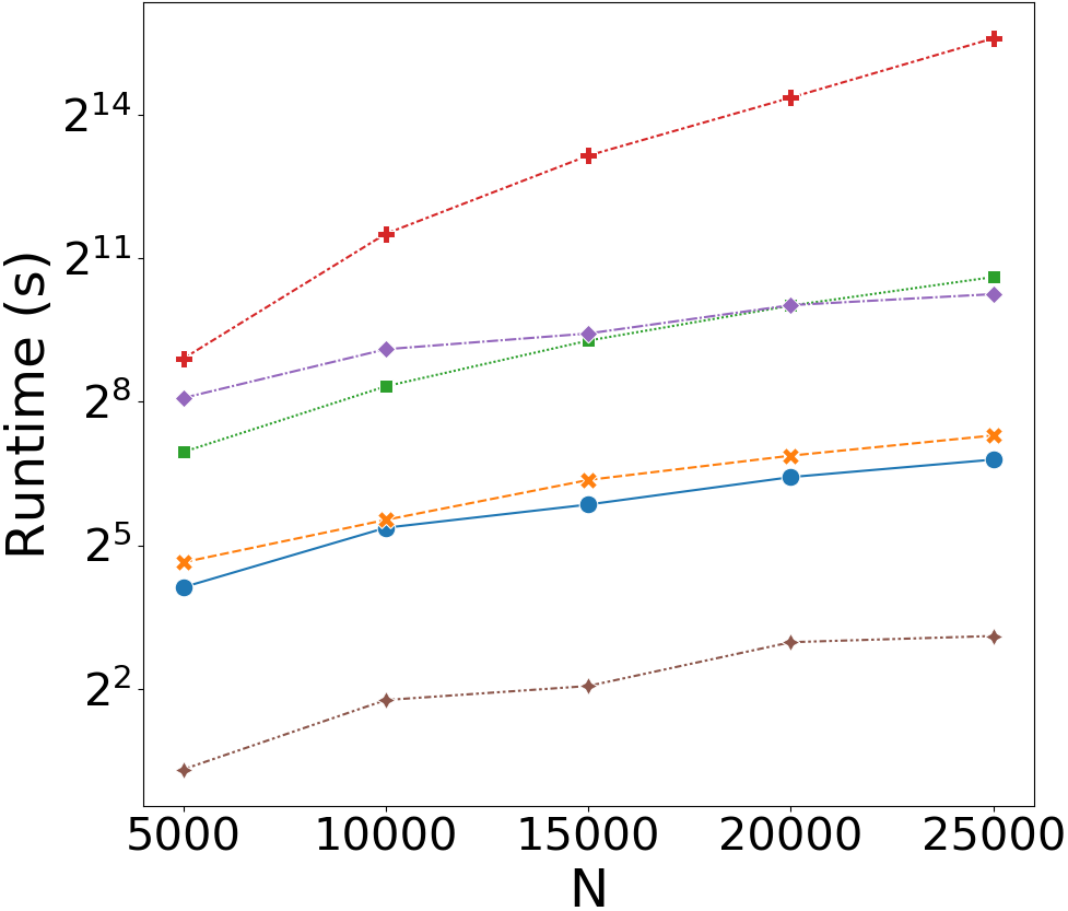
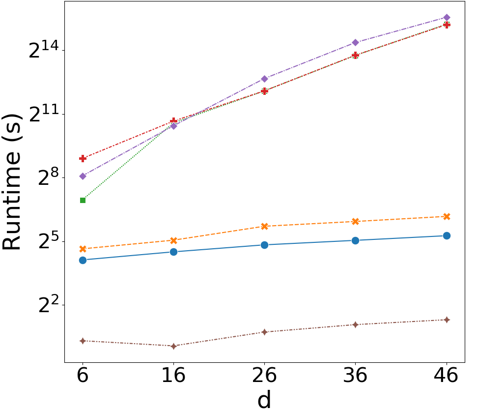
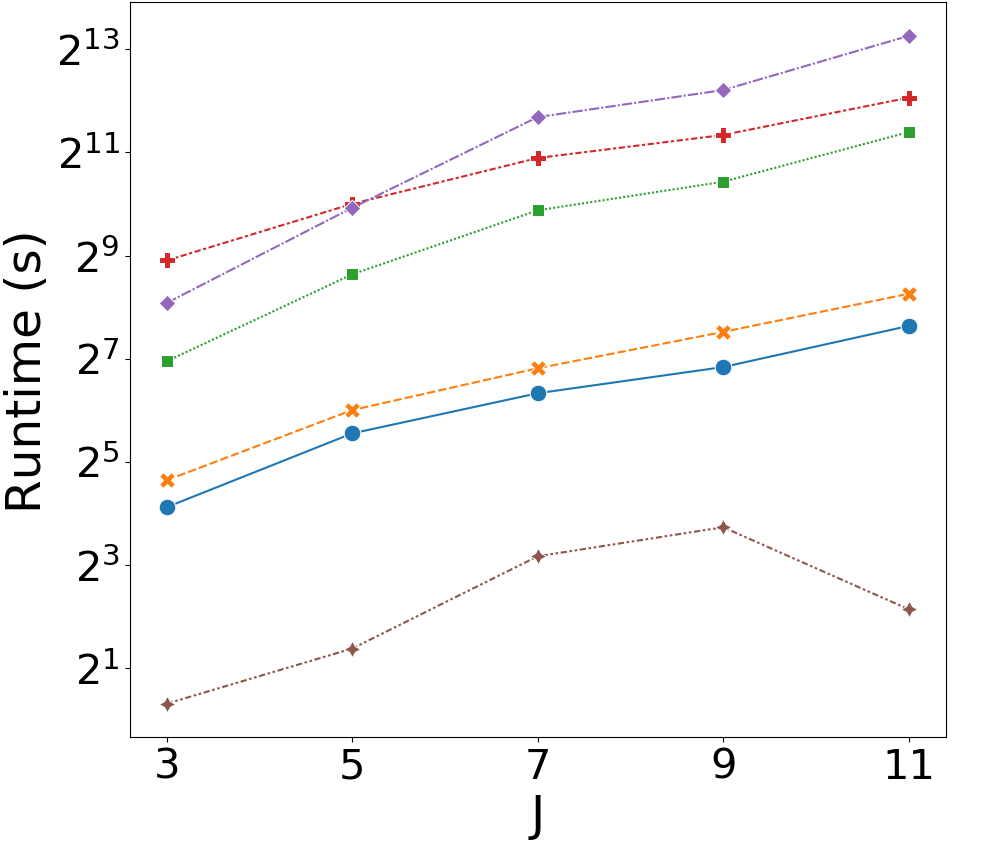
7 Runtime Analysis

We conduct runtime experiments on datasets with a rising number of objects $N$, dimensions $d$, and subspaces $J$. The created cluster spaces are always two-dimensional and contain three Gaussian clusters each.

All experiments are performed on a computer with an Intel Core i7-8700 3.2 GHz processor and 32GB RAM. The runtime results again correspond to the average of ten consecutive executions. The outcomes are illustrated in Figure 3.

The charts show that our approach is well applicable to high-dimensional datasets. The runtime increases only slightly with additional noise space dimensions (3(b)). ISAAC and MISC have to conduct an ISA which does not scale well to high-dimensional datasets. FOSSCLU has to perform Givens rotations multiple times, which is an expensive operation. On the other hand, our framework performs most steps in lower-dimensional subspaces where the overall dimensionality has no significant influence. If additional cluster spaces accompany a higher dimensionality, the runtimes of all algorithms behave similarly (3(c)). For large datasets, the differences in runtime are also much less prominent (3(a)). Only MISC needs significantly more time because a kernel graph regularized semi-nonnegative matrix factorization has to be performed.

Due to the additional operations required to calculate the outlier distance threshold for each subspace in each iteration, the execution of AutoNR with outlier detection expectably takes more time than without. Furthermore, the cluster centers and covariance matrices are updated after each outlier detection procedure.

NrDipmeans is the fastest in all experiments. However, it must be noted that NrDipmeans knows the correct number of subspaces and therefore does not need to run tests to identify $J$. Furthermore, in the case of $J=11$, it settles with the initial two clusters in each subspace and does not invest time in finding better structures. Therefore, it seems to have problems running with a high $J$. AutoNR, on the other hand, almost always correctly identifies all clusters in all subspaces.

Our procedure could be further accelerated by, for example, parallelizing the multiple executions of Nr-Kmeans with identical parameters.

8 Comparison to Nr-Kmeans

We perform additional experiments using the original Nr-Kmeans algorithm, to show that the good experimental results are based on our proposal and not merely on the integration of Nr-Kmeans. The new results are shown in Table 2. As in the paper, we repeated each experiment ten times and added the average score $\pm$ the standard deviation to the table.

Table 2: Results of AutoNR- and AutoNR+ compared to our Nr-Kmeans version, where the dimensionality of the noise space is determined through MDL (see supplement Section 5), and the original Nr-Kmeans implementation on various datasets. The left side shows the NMI results in %, the F1 results in % are shown on the right. All experiments were run ten times, and the average result $\pm$ the standard deviation is stated. The best algorithm for each subspace is marked in bold.

		NMI (%)				F1 (%)
Dataset	Subspace	AutoNR-	AutoNR+	Nr-Kmeans (MDL-based noise space)	Nr-Kmeans (Original)	AutoNR-	AutoNR+	Nr-Kmeans (MDL-based noise space)	Nr-Kmeans (Original)
syn3	1st ($k_{j}$=4)	$100\pm 0$	$100\pm 0$	$73\pm 20$	$59\pm 16$	$100\pm 0$	$100\pm 0$	$72\pm 18$	$61\pm 11$
(N=5000, d=11)	2nd ($k_{j}$=3)	$100\pm 0$	$100\pm 0$	$81\pm 13$	$75\pm 17$	$100\pm 0$	$100\pm 0$	$82\pm 12$	$78\pm 16$
	3rd ($k_{j}$=2)	$100\pm 0$	$100\pm 0$	$72\pm 22$	$75\pm 17$	$100\pm 0$	$100\pm 0$	$79\pm 16$	$81\pm 14$
syn3o	1st ($k_{j}$=4)	$86\pm 10$	$97\pm 0$	$62\pm 17$	$54\pm 13$	$83\pm 18$	$99\pm 0$	$64\pm 14$	$57\pm 10$
(N=5150, d=11)	2nd ($k_{j}$=3)	$90\pm 10$	$96\pm 0$	$67\pm 15$	$69\pm 11$	$91\pm 17$	$99\pm 0$	$73\pm 14$	$75\pm 9$
	3rd ($k_{j}$=2)	$77\pm 20$	$94\pm 0$	$56\pm 10$	$68\pm 13$	$80\pm 27$	$99\pm 0$	$63\pm 10$	$77\pm 13$
Fruits	Species ($k_{j}$=3)	$85\pm 9$	$83\pm 7$	$70\pm 14$	$74\pm 11$	$89\pm 9$	$87\pm 7$	$78\pm 11$	$78\pm 11$
(N=105, d=6)	Color ($k_{j}$=3)	$17\pm 2$	$18\pm 1$	$15\pm 2$	$16\pm 2$	$47\pm 3$	$44\pm 5$	$42\pm 3$	$44\pm 3$
ALOI	Shape ($k_{j}$=2)	$62\pm 4$	$64\pm 3$	$47\pm 26$	$54\pm 30$	$65\pm 2$	$65\pm 1$	$73\pm 13$	$77\pm 15$
(N=288, d=611)	Color ($k_{j}$=2)	$62\pm 4$	$64\pm 3$	$34\pm 0$	$31\pm 10$	$65\pm 2$	$65\pm 1$	$66\pm 0$	$66\pm 0$
DSF	Body-up ($k_{j}$=3)	$100\pm 0$	$100\pm 0$	$70\pm 20$	$81\pm 26$	$100\pm 0$	$100\pm 0$	$77\pm 16$	$85\pm 20$
(N=900, d=400)	Body-low ($k_{j}$=3)	$100\pm 0$	$100\pm 0$	$63\pm 22$	$56\pm 30$	$100\pm 0$	$100\pm 0$	$70\pm 17$	$68\pm 22$
CMUface	Identity ($k_{j}$=20)	$68\pm 4$	$64\pm 4$	$78\pm 6$	$75\pm 7$	$38\pm 4$	$34\pm 3$	$57\pm 9$	$52\pm 9$
(N=624, d=960)	Pose ($k_{j}$=4)	$35\pm 3$	$33\pm 1$	$28\pm 8$	$26\pm 6$	$45\pm 4$	$42\pm 4$	$41\pm 10$	$37\pm 10$
WebKB	Category ($k_{j}$=4)	$32\pm 2$	$34\pm 3$	$32\pm 3$	$30\pm 2$	$50\pm 5$	$58\pm 7$	$48\pm 3$	$48\pm 2$
(N=1041, d=323)	University ($k_{j}$=4)	$56\pm 4$	$57\pm 3$	$47\pm 8$	$45\pm 7$	$51\pm 2$	$52\pm 3$	$54\pm 7$	$52\pm 3$
NRLetters	Letter ($k_{j}$=6)	$100\pm 0$	$100\pm 0$	$85\pm 9$	$83\pm 9$	$100\pm 0$	$100\pm 0$	$78\pm 13$	$72\pm 12$
(N=10000, d=189)	Color ($k_{j}$=3)	$100\pm 0$	$100\pm 0$	$52\pm 29$	$39\pm 25$	$100\pm 0$	$100\pm 0$	$61\pm 22$	$52\pm 18$
	Corner ($k_{j}$=4)	$100\pm 0$	$100\pm 0$	$57\pm 26$	$48\pm 25$	$100\pm 0$	$100\pm 0$	$61\pm 23$	$51\pm 19$
Wine (N=178, d=13)	Type ($k_{j}$=3)	$76\pm 5$	$85\pm 3$	$87\pm 2$	$79\pm 15$	$81\pm 6$	$90\pm 4$	$92\pm 2$	$87\pm 10$
Optdigits (N=5620, d=64)	Digit ($k_{j}$=10)	$73\pm 1$	$74\pm 1$	$72\pm 2$	$70\pm 2$	$54\pm 4$	$58\pm 4$	$66\pm 3$	$64\pm 3$

AutoNR returns superior results in most experiments, even though Nr-Kmeans already knows the correct number of subspaces and clusters for each subspace. Only for the non-redundant dataset ALOI does the original Nr-Kmeans perform better regarding the F1 score. This case, however, has already been mentioned in the paper. The biggest advantage of our application is the fact that it discovers structures one by one while preserving the ability to adjust already found subspaces. This gives great flexibility, so that possible errors can be compensated in a following iteration. Another advantage is the definition of the noise space using MDL (see supplement Section 5), as it can be seen with the datasets CMUface, WebKB, NRLetters, Wine and Optdigits.

One could argue that the multiple repetitions of Nr-Kmeans included in each run of AutoNR strongly favor our algorithm. However, we would like to counter this by stating that Nr-Kmeans by itself is often unable to achieve a perfect result just once (e.g., for syn3). In contrast, AutoNR often assigns the points to the correct clusters every time. This shows that the iterative identification of subspaces can be beneficial, with the effect becoming stronger the more subspaces there are.

9 Importance of Correct Parametrization

Figure 4: Results of various parametrizations of Nr-Kmeans on NRLetters. $k_{1}$ is set to $6$. The left image shows the NMI, and the right the F1 results.

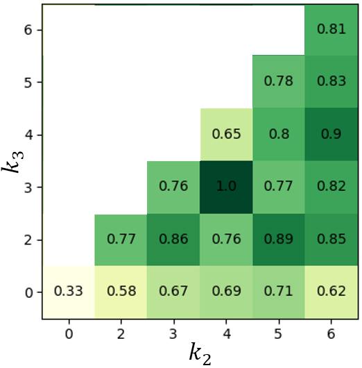
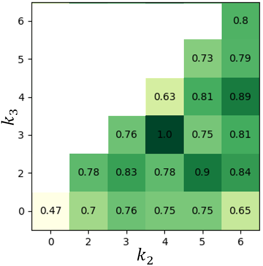
To better assess the importance of a correct parametrization of non-redundant clustering approaches, we perform another experiment. Suppose that we know that NRLetters comprises six different letters. We know nothing about the other clustering possibilities. Therefore, we try different parameters for Nr-Kmeans using a brute-force search. Here, we assume that no subspace contains more than six clusters. The NMI and F1 results can be seen in Figure 4. To arrive at a single number that indicates the quality of a non-redundant clustering result, we compute the average result over all three subspaces.

$$\text{score}(R^{gt},R^{p})=\frac{1}{J_{gt}}\sum_{1\leq j\leq J_{gt}}\textit{score}_{j}(R^{gt},R^{p}),$$

where $\textit{score}_{j}(R^{gt},R^{p})$ is the evaluation method as described in the paper and $J_{gt}$ is the number of label sets in the ground truth. Each run is repeated ten times and the best result is added to the heatmap.

We see that the quality of the results deteriorates away from the optimum ($k_{2}=4,k_{3}=3$) even though we know the correct number of clusters in the first subspace. This shows the value of our framework, which achieved a perfect result in all ten iterations and that, without prior knowledge.

References

- [1] D. Arthur and S. Vassilvitskii, k-means++: The advantages of careful seeding, in 18th ACM-SIAM SODA, Society for Industrial and Applied Mathematics, 2007, pp. 1027–1035.
- [2] S. Goebl, X. He, C. Plant, and C. Böhm, Finding the optimal subspace for clustering, in 14th IEEE ICDM, IEEE, 2014, pp. 130–139.
- [3] S. Günnemann, I. Färber, M. Rüdiger, and T. Seidl, Smvc: semi-supervised multi-view clustering in subspace projections, in 20th ACM SIGKDD, 2014, pp. 253–262.
- [4] J. Hu, Q. Qian, J. Pei, R. Jin, and S. Zhu, Finding multiple stable clusterings, Knowledge and Information Systems, 51 (2017), pp. 991–1021.
- [5] T. C. Lee, An introduction to coding theory and the two-part minimum description length principle, International statistical review, 69 (2001), pp. 169–183.
- [6] D. Mautz, W. Ye, C. Plant, and C. Böhm, Discovering non-redundant k-means clusterings in optimal subspaces, in 24th ACM SIGKDD, 2018, pp. 1973–1982.
- [7] D. Mautz, W. Ye, C. Plant, and C. Böhm, Non-redundant subspace clusterings with nr-kmeans and nr-dipmeans, ACM Transactions on Knowledge Discovery from Data (TKDD), 14 (2020), pp. 1–24.
- [8] X. Wang, J. Wang, C. Domeniconi, G. Yu, G. Xiao, and M. Guo, Multiple independent subspace clusterings, in AAAI, vol. 33, 2019, pp. 5353–5360.
- [9] W. Ye, S. Maurus, N. Hubig, and C. Plant, Generalized independent subspace clustering, in 16th IEEE ICDM, IEEE, 2016, pp. 569–578.