Stability of Multi-Agent Learning in Competitive Networks:
Delaying the Onset of Chaos
Abstract
The behaviour of multi-agent learning in competitive network games is often studied within the context of zero-sum games, in which convergence guarantees may be obtained. However, outside of this class the behaviour of learning is known to display complex behaviours and convergence cannot be always guaranteed. Nonetheless, in order to develop a complete picture of the behaviour of multi-agent learning in competitive settings, the zero-sum assumption must be lifted.
Motivated by this we study the Q-Learning dynamics, a popular model of exploration and exploitation in multi-agent learning, in competitive network games. We determine how the degree of competition, exploration rate and network connectivity impact the convergence of Q-Learning. To study generic competitive games, we parameterise network games in terms of correlations between agent payoffs and study the average behaviour of the Q-Learning dynamics across all games drawn from a choice of this parameter. This statistical approach establishes choices of parameters for which Q-Learning dynamics converge to a stable fixed point. Differently to previous works, we find that the stability of Q-Learning is explicitly dependent only on the network connectivity rather than the total number of agents. Our experiments validate these findings and show that, under certain network structures, the total number of agents can be increased without increasing the likelihood of unstable or chaotic behaviours.
Introduction
Multi-Agent Learning in competitive games requires agents to maximise their individual, competing rewards whilst simultaneously exploring their actions to find optimal strategies. This leads to a highly non-stationary problem where agents must react to the changing behaviour of adversarial agents. The study of Multi-Agent Learning in competitive settings has achieved a number of successes within the context of zero-sum games and their network variants These games model perfect competition between agents, yielding an underlying structure which make them amenable for studying multi-agent learning. In particular it is known that certain learning dynamics asymptotically converge to an equilibrium in network zero-sum games (Ewerhart and Valkanova 2020; Leonardos, Piliouras, and Spendlove 2021; Kadan and Fu 2021) whilst others converge in time average (Anagnostides et al. 2022; Hadikhanloo et al. 2022; Bailey and Piliouras 2019).
Yet in practice the requirement of an arbitrary competitive game to exactly satisfy the zero-sum condition is restrictive. It therefore becomes important to study the behaviour of learning agents in arbitrary competitive games.The challenge in taking this step is that there are infinitely many realisations of games which can be considered competitive, making a case by case analysis intractable. Furthermore, the non-stationarity of learning in competitive games often leads to complex behaviours such as cycles (Galla 2011; Mertikopoulos, Papadimitriou, and Piliouras 2018) and even chaos (Griffin, Semonsen, and Belmonte 2022; Sato, Akiyama, and Farmer 2002). In fact, recent work has shown that chaotic dynamics occur in games even slightly perturbed from the zero-sum setting (Galla and Farmer 2013; Sato, Akiyama, and Farmer 2002). In addition, recent work (Hussain, Belardinelli, and Piliouras 2023; Sanders, Farmer, and Galla 2018) has shown that the ability of learning dynamics to reach an equilibrium with low exploration rates diminishes as the number of agents increases. These technical challenges present a strong barrier towards ensuring the convergence of learning in competitive games with many players.
However, in both (Hussain, Belardinelli, and Piliouras 2023) and (Sanders, Farmer, and Galla 2018) it was assumed that all agents are directly influenced by all other agents in the environment. In practice, however, this does not hold. Many ML applications, including Generative Adversarial Networks (GANs) enforce structured interactions between models (Hoang et al. 2018; LI et al. 2017). Furthermore, real world problems such as robotic systems (Hamann 2018; Shokri and Kebriaei 2020) and competitive game playing (Perolat et al. 2022) impose a communication network between agents. In economic settings, agents interact through social networks either online or in communities.
Model and Contributions
Motivated by this, we study multi-agent learning in network games, in which interactions between agents are modelled by an underlying communication network. In this setting, we study the Q-Learning dynamic (Sato and Crutchfield 2003; Tuyls, Hoen, and Vanschoenwinkel 2006), a foundational model for studying the behaviour of agents who explore their state space, whilst simultaneously exploiting their rewards.
To address the issue of studying generic competitive games, we take a statistical approach towards our analysis which is inspired by the study of ecological systems (Opper and Diederich 1992; Galla 2006) and statistical mechanics (Hertz, Roudi, and Sollich 2016; De Giuli and Scalliet 2022). Rather than engaging in a case-by-case analysis, we parameterise competitive network games by the strength of anti-correlation between agent payoffs. Then, we perform a kind of average case analysis over all games which are drawn from this parameter. This process has shown a number of success in the analysis of learning in games (Galla and Farmer 2013; Sanders, Farmer, and Galla 2018; Coolen 2005) and neural networks (Coolen 2001; Kadmon and Sompolinsky 2015; Sompolinsky, Crisanti, and Sommers 1988).
Our analysis allows us to determine how the stability of the Q-Learning dynamics is influenced by the competitiveness of the game and on the exploration rate. In particular, we are able to define a stability boundary in terms of these parameters. We find that stable behaviours occur with low exploration rates in highly competitive games, such as zero-sum games. However, as the game deviates further from perfect competition, higher exploration rates are required to ensure convergent behaviours. We also analyse how the network itself influences Q-learning dynamics. We find that complex dynamics occurs frequently in strongly connected networks as the number of agents increases. By contrast, there are networks for which the total number of agents has no influence on the asymptotic convergence of learning.
The statistical approach requires taking the limit of large action spaces. As a result, our theoretical stability boundary holds exactly in this limit. However, we evaluate its predictions through rigorous numerical experiments in finite games, including representative examples from the literature. We find that the experiments agree with the theoretical results and show that the likelihood of complex learning dynamics depends explicitly on the network structure rather than the total number of agents. In fact it is found that, as long as the network is chosen appropriately, an arbitrarily large number of agents can be added to the multi-agent system without compromising convergence of learning.
Related Work
A number of recent advances in the theory of learning in games have drawn from tools in evolutionary game theory (Hofbauer and Sigmund 1998, 2003; Tuyls 2023). Here, popular learning algorithms such as Q-Learning (Sutton and Barto 2018), Follow-the-Regularised-Leader (Shalev-Shwartz 2011) and Fictitious Play (Brown P 1949) can be approximated by continuous time models (Tuyls, Hoen, and Vanschoenwinkel 2006; Mertikopoulos and Sandholm 2016). Then, tools from the study of continuous dynamical systems (Strogatz 2015; Meiss 2007) can be used to analyse the asymptotic behaviour of the learning dynamic. In this manner, strong predictions can be made regarding convergence of learning in games (Krichene 2016; Abe, Sakamoto, and Iwasaki 2022; Bloembergen et al. 2015; Perolat et al. 2020). Notable successes of this method lie in network zero sum games (Cai et al. 2016; Abernethy, Lai, and Wibisono 2021) which models perfect competition between agents. In this setting, it is known that a number of learning dynamics converge asymptotically to an equilibrium (Leonardos, Piliouras, and Spendlove 2021; Ewerhart and Valkanova 2020; Kadan and Fu 2021).
By contrast, few guarantees can be provided outside of this class (Anagnostides et al. 2022). In fact, complex behaviour such as limit cycles (Imhof, Fudenberg, and Nowak 2005; Galla 2011; Mertikopoulos, Papadimitriou, and Piliouras 2018) and chaos (Sanders, Farmer, and Galla 2018; van Strien and Sparrow 2011) are known to be prevalent in generic games. To make progress on this front, learning in games has benefited from tools derived from the study of disordered systems (Hertz, Roudi, and Sollich 2016). The premise is that the exact choice of rewards in generic games has infinitely many possible realisations. Therefore, it becomes necessary to parameterise the game and then analyse the average behaviour of the learning dynamic under all games which share the same parameter. This analysis has been successful in the analysis of ecological systems (Opper and Diederich 1992; De Giuli and Scalliet 2022), Recurrent Neural Networks, (Coolen 2001) and evolutionary game theory (Coolen 2005; Chowdhury et al. 2021).
Most similar to our work are (Galla and Farmer 2013; Sanders, Farmer, and Galla 2018). In the former, the authors analysed two player competitive games and studied Experience Weighted Attraction (EWA) (Camerer and Ho 1999), a learning algorithm closely related to Q-Learning (Leonardos, Piliouras, and Spendlove 2021). They were able to derive a boundary in terms of game competitiveness and exploration rate between stable learning dynamics and complex dynamics. In (Sanders, Farmer, and Galla 2018), the authors extended this work towards multi-player games in which each agent interacts with all others. In this setting, it was shown the stability boundary depends on the total number of agents in the game. In particular, the region in which learning converges to fixed point seems to vanish as the number of agents increases. This result is supported by that of (Hussain, Belardinelli, and Piliouras 2023) in which a lower bound on exploration rates was determined so that Q-Learning dynamics converge to a unique equilibrium. Again it was shown that this lower bound increases with the number of agents.
In this work, we refine the result of (Sanders, Farmer, and Galla 2018) towards the setting of generic network games. Importantly, we find that the stability boundary is independent of the total number of agents in the game, but rather explicitly dependent on the connectivity of the network.
Preliminaries
Game Model
A network polymatrix game (henceforth network game) is described by a tuple . Here, denotes a set of agents indexed by , and denotes the set of edges in an underlying network. In particular, if agents and are connected in the network. The set of neighbours of an agent is denoted by . Associated with each edge are the payoff matrices , where denotes the number of actions an agent can play. The set of actions playable by agent is indexed by . The strategy of agent is a probability distribution over their set of actions and so is chosen from the -simplex . Then for any agent , given the joint strategy of their opponents, their total reward is given by
| (1) |
In words, it is the sum of the payoff they receive in each of the games played along their edges. With this in place we can define an equilibrium for the game as follows.
Definition 1 (Quantal Response Equilibrium (QRE)).
A joint mixed strategy is a Quantal Response Equilibrium (QRE) if, for all agents and all actions
where denotes the exploration rate of all agents.
The QRE (Camerer, Ho, and Chong 2004) is the prototypical extension of the Nash Equilibrium to the case of agents with bounded rationality, parameterised by the exploration rate . In particular, the limit corresponds exactly to the Nash Equilibrium, whereas the limit corresponds to a purely irrational case, where the QRE is unique and lies at the uniform distribution (McKelvey and Palfrey 1995).
Payoff Correlations
As mentioned in the introduction, the entries of can take any value in , making a case-by-case analysis intractable. We therefore move towards a kind of average case analysis. In particular, we construct ensembles of games at random which are parameterised by the strength of anti-correlation between opponent payoffs. Then we can analyse the expected behaviour of Q-Learning dynamics for different choices of this parameter. This approach has yielded a number of successes in analysing replicator dynamics (Opper and Diederich 1992) and learning in games (Galla and Farmer 2013; Sanders, Farmer, and Galla 2018).
Averaging over the infinite possibilities of payoff matrices which could arise in a game theoretic setting has the immediate effect of reducing the information available regarding the effect of the payoffs on stability. However, the primary concern of this work is to understand the effect of the network structure on stability. As such, it makes sense to average over other factors. Indeed, the relevance of the payoff matrices on the learning dynamics is an open and important topic for research and we point the interested reader to (Pangallo, Heinrich, and Farmer 2019; Pangallo et al. 2022) for rigorous treatments on the matter.
We must then ask how best to parameterise the payoffs. We do this by invoking the maximum entropy principle which is foundational to statistical mechanics (Galla and Farmer 2013; Hertz, Roudi, and Sollich 2016). This states that the natural choice for the payoff matrices is that which maximises entropy subject to given conditions. In particular, these conditions are
| (2) | ||||
Intuitively, these conditions enforce that payoffs have zero mean and positive variance and, crucially, enforces a correlation between the payoffs between two connected agents parameterised by . In the Supplementary Material we discuss, as an example, games which are drawn with . Here, the payoffs to each agent are exactly negatively correlated, corresponding to a zero-sum game. By contrast, when , the payoffs are completely uncorrelated. As such, controls the competitiveness of the game. In line with the maximum entropy argument and previous literature (Galla and Farmer 2013; Sanders, Farmer, and Galla 2018), we draw the payoff matrices from a multivariate Gaussian distribution with mean and covariance defined as in (Payoff Correlations). A careful treatment on why the multivariate distribution satisfies the maximum entropy argument can be found in (Galla and Farmer 2013). Furthermore, as we show in our experiments(and in line with previous studies on the analysis of random games (Galla and Farmer 2013; Sanders, Farmer, and Galla 2018)), the predictions made in the average case analysis of random games carries over strongly in experiments.
Learning Model
In this work, we analyse the Q-Learning dynamic, a prototypical model for determining optimal policies by balancing exploration and exploitation. In this model, each agent maintains a history of the past performance of each of their actions. This history is updated via the Q-update:
where denotes the current time step, and denotes the Q-value maintained by agent about the performance of action . In effect gives a discounted history of the rewards received when is played, with as the discount factor.
Given these Q-values, each agent updates their mixed strategies according to the Boltzmann distribution, given by
in which is the exploration rate of all agents.
It was shown in (Tuyls, Hoen, and Vanschoenwinkel 2006; Sato and Crutchfield 2003) that a continuous time approximation of the Q-Learning algorithm could be written as
| (QLD) |
which we call the Q-Learning dynamics (QLD). The fixed points of this dynamic coincide with the QRE of the game (Leonardos, Piliouras, and Spendlove 2021). We can rewrite the dynamic in the following form
| (3) | ||||
| (4) |
In this light, can be seen as a normalisation factor which ensures that . In addition, it is clear that the behaviour of the Q-Learning dynamics depend strongly on the choice of , the structure of the edge set , and the payoffs . In (Sanders, Farmer, and Galla 2018), a variant of (QLD) was analysed in which the concept of the interaction network was not introduced. Rather, each agent would be required to play a single -player game against all other agents in the environment. In their work, it was found that complex dynamics (cycles and chaos) becomes more prominent as the number of players in the game increases. This is similarly true of (Hussain, Belardinelli, and Piliouras 2023) in which (QLD) was analysed in arbitrary games, without imposing any structure on interactions between agents. The authors similarly concluded that, as the number of agents increases, higher exploration rates are required to ensure convergence to a QRE.
The introduction of a communication network allows for the interactions between agents to be included in the study. In particular, we determine how the number of neighbours for each agent affects the stability of (QLD) and compare this with the total number of players. In this light, we make the following assumption.
Assumption 1.
The agents all share the same number of neighbours , i.e., . In graph theoretic terms, we require that the network is regular (Ji and Egerstedt 2007).
Assumption 1 allows us to parameterise the connectivity of the network using only the number of neighbours . Additionally it allows us to make a direct comparison of our results with that of (Sanders, Farmer, and Galla 2018) who study the case where all agents are connected, in our case this is . Whilst the study of regular networks is certainly well motivated in the literature on multi-agent systems (Ji and Egerstedt 2007; Rahmani et al. 2009; Olfati-Saber, Fax, and Murray 2007), a fruitful direction for extending the work in this paper would be to introduce graph theoretic parameterisations (e.g. norms on the adjacency matrix) to include heterogeneously coupled networks in the analysis.
Statistical Analysis of Learning in Networks
In this section, we derive a necessary condition for (QLD) to converge in generic network games. The process for doing this is as follows. First, we average over the ensemble of games drawn using a particular choice of . This allows us to define an effective dynamic, which reflects the expected behaviour of (QLD) over all games within the ensemble. Then, we determine a necessary condition for a fixed point of this dynamic to be stable. Similar calculations have been used to analyse replicator dynamics (Galla 2006; Opper and Diederich 1992) and variants of Q-Learning (Sanders, Farmer, and Galla 2018; Galla and Farmer 2013), as well as minority games (Coolen 2005) and recurrent neural networks (Coolen 2001). By following this process, we derive an estimate for the boundary between stable fixed points and other behaviours, such as limit cycles and chaos. This boundary is determined with respect to the payoff correlations and the exploration rate .
The analytic result requires applying techniques from statistical mechanics, where the theory holds exactly only in the limit of large payoff matrices, i.e., the number of actions . As shown in this Section the method allows us to isolate precisely how the number of neighbours and the total number of players affects the stability of learning in arbitrary competitive games. The limitation is that the analytic result will overestimate the stability boundary for finite games. However, our numerical experiments show that the predictions made in the limit hold in practice for finite games.
Effective Dynamics
In our first step, we derive an effective dynamics which describes the expected behaviour of the Q-Learning dynamics averaged over all possible assignments of payoff matrices. This calculation is lengthy, so we report the full details in the Supplementary Material. The idea is to define a probability measure (Generating Functional described in the Appendix) over trajectories generated by Q-Learning dynamics, given some payoff matrices. Next, we invoke the assumption that the payoff matrices are drawn from a multivariate Gaussian with correlations parameterised by . Using this, we find the average form of the probability measure over all games generated with a choice of , which we call its effective form. It is here that we use the limit of large payoff matrices (number of actions ). Finally, we identify the effective probability measure with an associated dynamical system, which we call the effective form for the Q-Learning dynamics. Intuitively, the effective Q-Learning dynamics (5) describes the average trajectories of Q-Learning over all, possibly infinite, games which are generated from a choice of .
| (5) |
Here, is a Gaussian random variable which satisfies and . Following (Opper and Diederich 1992), we use to denote an average taken over all possible realisations of payoffs drawn using a choice of . Similarly, is a random variable satisfying As such, and capture the time correlations between the strategy at times and . We assume, as part of our derivation, that the initial conditions for all agent strategies are independently and identically distributed (i.i.d) and so we drop the distiction between agents and actions in (5).
Stability Analysis
Next, we determine the stability of fixed points for the effective dynamics. To do this, we write where denotes a fixed point of (5) and denotes perturbations due to an additive white noise term which is drawn from a Gaussian of zero mean and unit variance. Similarly we write where gives perturbations in the time correlation variable due to the random noise. The problem of determining stability of fixed points is now a question of the growth or decay of close to the fixed point . To do this, we only need to keep terms in (5) which are linear in . This yields
| (6) | ||||
where we also account for the fact that, at the fixed point time correlations are constant so that , which we rewrite as .
Since (6) contains a convolution term , a classical eigenvalue analysis is intractable as an approach to determining stability. Instead, we adopt the procedure presented in (Opper and Diederich 1992) which we now outline, with full details given in the Supplementary Material. We first take the Fourier transform of (6). Doing so yields an equation in terms of frequency rather than time and reduces the convolution term into a product. In particular we obtain
| (7) | ||||
where we overload notation by identifying each variable with its Fourier Transform, e.g. . This leads to the relation
where we recall again that denotes an expectation over all realisations of the effective dynamics from an ensemble of games drawn with the same choice of . In order to analyse asymptotic stability, we focus on the limit , since this corresponds to longer timescales in . Finally, we apply the relation to write the dynamic solely in terms of . This gives
| (8) |
By definition, the left hand side of (8) is positive, so a contradiction is reached if
| (9) |
where . As a result, (9) defines a sufficient condition for the onset of instability in the effective dynamics.
Discussion
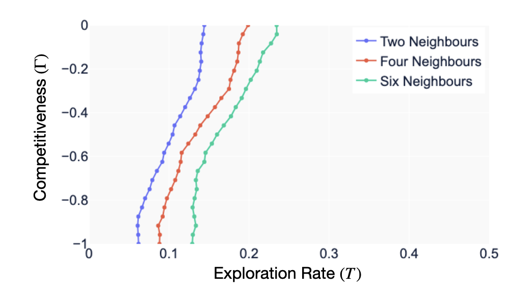
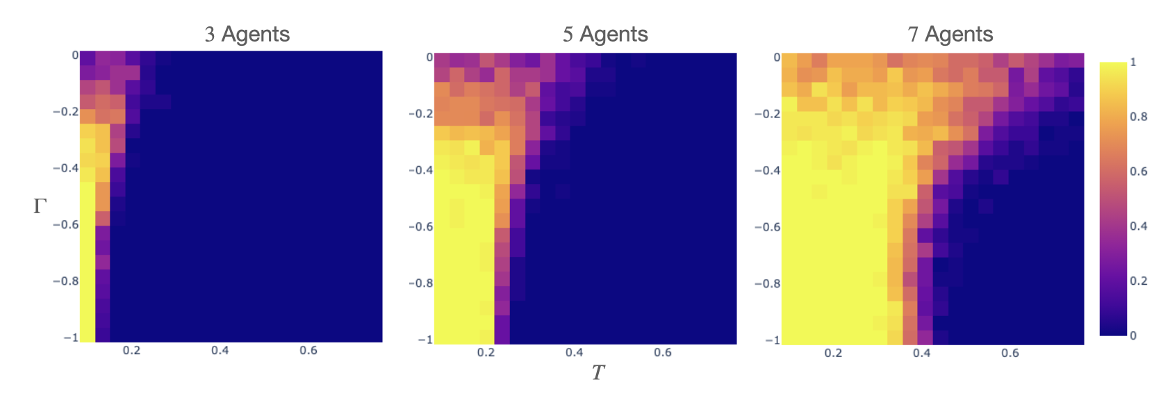
In general, the stability condition (9) is not straightforward to parse and cannot be solved in closed form. This is mostly due to the dependence on the fixed point , whose form can be complicated. Nevertheless, it is possible to numerically estimate the location of the stability boundary, i.e., the boundary between choices of which satisfy (9) and those which do not. To do this, we fix a choice of , iteratively solve for and subsequently evaluate (9). Repeating this procedure for many choices of yields the stability boundary depicted in Figure 1, in which each line depicts the transition from satisfying the condition (9) on the right to its violation on the left. By examining this we can assess how each of the parameters influence the stability of Q-Learning Dynamics.
The most notable feature of the necessary condition for stability (9) is the dependence on the number of neighbours . Even from (9) itself we can discern the explicit independence on the total number of agents , which does not appear anywhere in the condition. Therefore, in competitive games, the stability of learning is not influenced by the total number of agents, so long as the number of neighbours per agent is kept constant. By contrast, as the number of neighbours increases the unstable region occupies more of the parameter space.
This result refines that of (Sanders, Farmer, and Galla 2018) in which a stability boundary was determined for multi-player games without any underlying communication structure. In this setting the authors showed that increasing number of players leads to a larger unstable region. In our setting, this corresponds to a fully connected network in which . From Figure 1 it is clear that our result yields the same prediction. Similarly, (9) aligns exactly with the result of (Galla and Farmer 2013) which derives a stability boundary in two-player games. In our case this corresponds to any network game in which .
Another feature shown by Figure 1 is that the stability boundary increases in as decreases from to . That is, as the strength of anticorrelation between agent payoffs decreases, higher exploration rates are required for Q-Learning dynamics to settle to an equilbrium. Recall that corresponds to case where games along each edge are exactly negatively correlated, i.e., a zero-sum game. From (Leonardos, Piliouras, and Spendlove 2021) it is known that that Q-Learning dynamics asymptotically converge in network games which are exactly zero-sum for any positive value of . Figure 1 shows that, as the competitiveness of the game decreases (i.e., as ), higher exploration rates are required to guarantee convergence.
Experiments
In this section we test the validity of the predictions made in our theoretical analysis in the case of games with finite action sets by running the Q-Learning algorithm, outlined in the Preliminaries.
Representative Examples of Networks
In our experiments we analyse two examples of networks - the ring network and the fully connected network. These act as prototypical examples for regular networks, which satisfy Assumption 1. In the former, the payoff for any agent is given by
where addition and subtraction are taken . In this case, each agent has only two neighbours, i.e. so the network connectivity is independent of the total number of agents . In the fully connected network, the payoff is given by
so that each agent has neighbours. This corresponds also to the case analysed by (Sanders, Farmer, and Galla 2018) and (Hussain, Belardinelli, and Piliouras 2023) in which it was predicted that the boundary between stable and unstable learning dynamics is impacted by the total number of agents.
Example: Network Sato Game
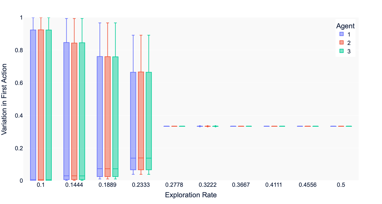
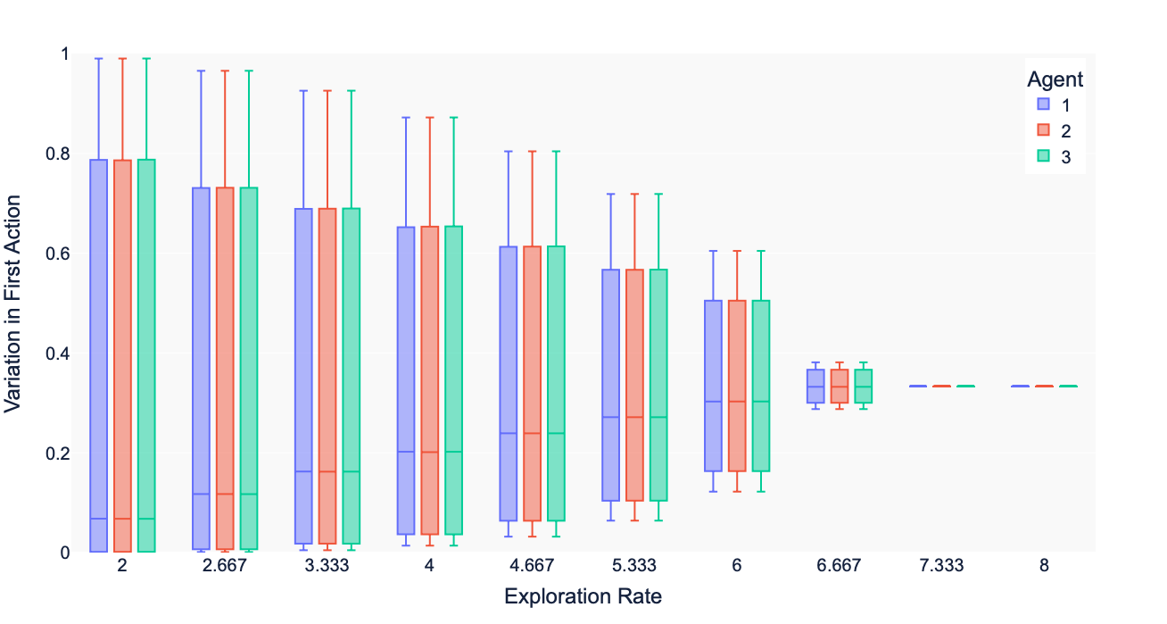
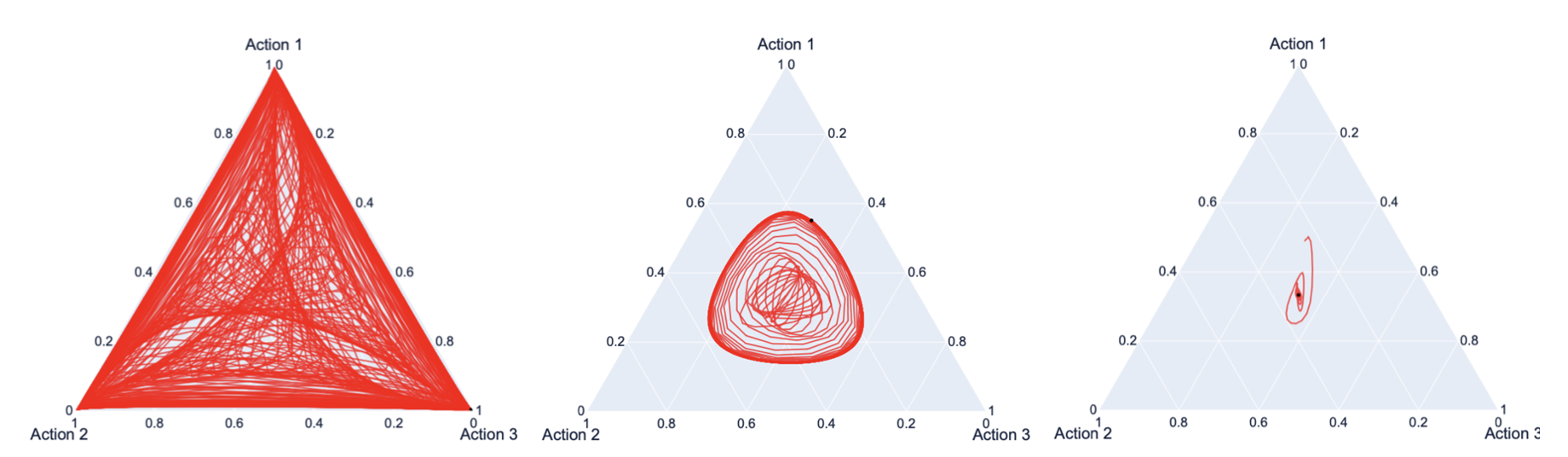
We first illustrate the behaviour of Q-Learning on a representative example. This is an extension of the variant of Rock-Paper-Scissors first examined in (Sato, Akiyama, and Farmer 2002). The network extension is described in the Supplementary Material, alongside visualisations of chaotic trajectories generated by Q-Learning. In Figure 2, we simulate 50 agents playing the Network Sato Game. We record the agents’ mixed strategies in the final iterations of Q-Learning and, for three representative agents, plot the probabilities with which they play their first action. As such, Figure 2 depicts the spread of the asymptotic trajectory over the simplex. It is clear that, in the fully connected network, a large value of is required in order for the agents to converge to an equilibrium, whereas in the ring network is sufficient.
Arbitrary Finite Games
Next, we determine the correctness of the analytic result in arbitrary games. In Figure 3, we draw games with actions for each agent given choice of using the formulation in Payoff Correlations. Once again, we simulate Q-Learning dynamics for time steps and record the final iterations. To characterise the limiting behaviour, we apply the following heuristic. We first determine whether, for each agent and each strategy component, the relative difference between the maximum and minimum value across all 10000 time-steps is less than . Formally, we determine whether
where is taken over the final 10000 iterations of learning. Next, we determine the variance across the final iterations as
| (10) |
We check if the variance is less than . If both of the above conditions are met, then the dynamic is considered to have converged. As an example, the convergent dynamics in Figure 2 satisfy both of these conditions. If, across all 10000 time steps, there is some such that, for all agents and all , , , , are all within of each other, then it is considered that a stable periodic orbit has been reached.
If neither of these conditions are met, then the dynamic is deemed to be non-convergent. Note this does not conclude that the dynamics are formally chaotic, as limit cycle behaviours are also known to occur in learning (Mertikopoulos, Papadimitriou, and Piliouras 2018; Imhof, Fudenberg, and Nowak 2005). Examples of such behaviours are displayed in the Supplementary Material. However, in (Galla and Farmer 2013; Sanders, Farmer, and Galla 2018) Q-Learning dynamics were shown to exhibit chaotic behaviour for certain choices of . This is also in line with the rich literature on chaos in multi-agent learning (Sato, Akiyama, and Farmer 2002; Mukhopadhyay and Chakraborty 2020; van Strien and Sparrow 2011).
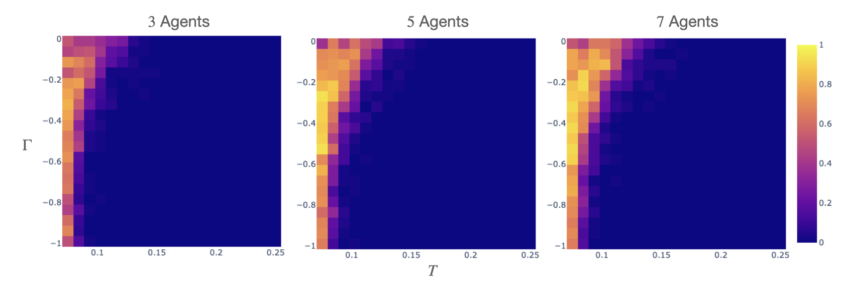
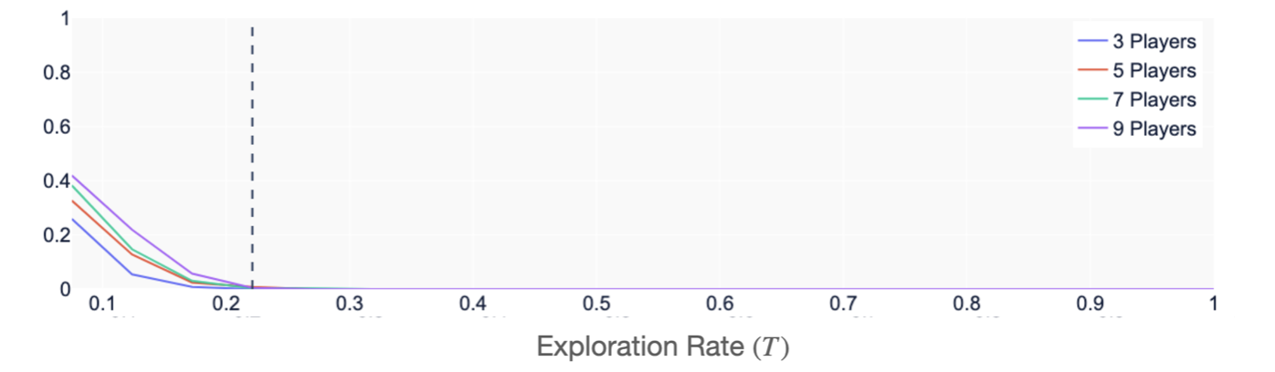
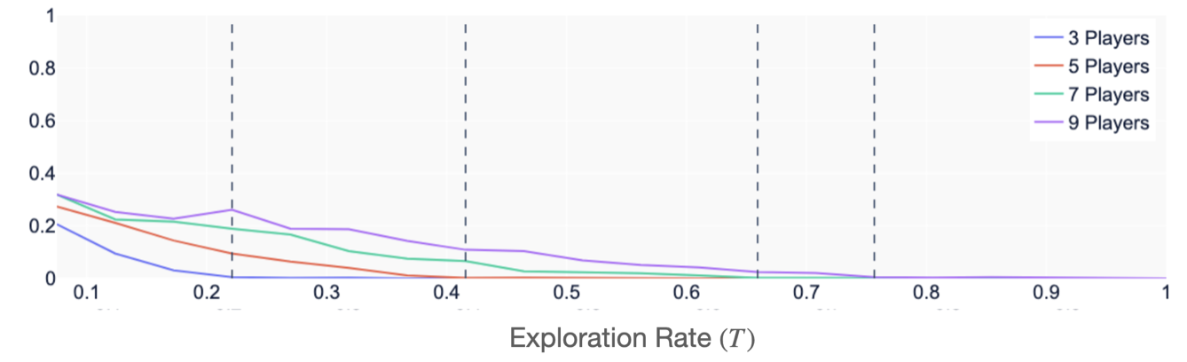
From Figure 3, it can be seen that the form of the analytic stability boundary holds in practice. The reason that the empirical boundary overestimates the theoretical result is that the latter considers asymptotic trajectories, i.e. infinite time-scales, whilst the former is evaluated over 75,000 steps. Therefore, in the experiments, slow convergence can be mistaken for non-convergence. Overall, however, we see a strong alignment between the theoretical predictions and experimental evaluation. Namely, lower exploration rates are required strictly competitive games, i.e. as , whilst uncorrelated games require higher exploration rates in order to converge to an equilibrium. In addition, the stability boundary is unaffected by the number of players in the ring network.
The latter point is highlighted in Figure 4 in which we average over multiple choices of to isolate the effect of the number of neighbours on the stability boundary in terms of . It is evident that increasing the number of players in a ring network plays no impact on the stability boundary. As a result, it is possible to increase the number of agents in such games arbitrarily without compromising convergence of Q-Learning to a fixed point. By contrast fully connected networks do not scale well, as non-convergent behaviours remain prevalent for low values of as the number of agents increase.
Conclusion
In this study we have refined the previously held belief that chaotic behaviours are more prevalent in games with many players. In particular, we analyse network games and show that stability of the Q-Learning dynamic depends on the structure of the network, the competitiveness of the game and the exploration rates of agents. We show that in certain networks, such as the ring network, an arbitrary number of agents may be added to the system without compromising the propensity for learning to converge. By contrast, if agents are heavily connected in the network, non-convergent behaviours, such as limit cycles and chaos, become prevalent even with a small total number of agents.
The present work has isolated the effect of the number of neighbours and the number of players in the game. However, there are other factors which may affect the stability of Q-Learning. For instance, whilst we have required to be the same for all agents, it would be fruitful to analyse heterogeneously coupled networks. More generally, tools from graph theory may be applied within this framework to uncover the role of the network in convergence for arbitrary network games. Our work, therefore, presents a first step towards building a complete picture of the stability of multi-agent learning in network games.
Acknowledgments
Aamal Hussain and Francesco Belardinelli are partly funded by the UKRI Centre for Doctoral Training in Safe and Trusted Artificial Intelligence (grant number EP/S023356/1)
References
- Abe, Sakamoto, and Iwasaki (2022) Abe, K.; Sakamoto, M.; and Iwasaki, A. 2022. Mutation-driven follow the regularized leader for last-iterate convergence in zero-sum games. In Cussens, J.; and Zhang, K., eds., Proceedings of the Thirty-Eighth Conference on Uncertainty in Artificial Intelligence, volume 180 of Proceedings of Machine Learning Research, 1–10. PMLR.
- Abernethy, Lai, and Wibisono (2021) Abernethy, J.; Lai, K. A.; and Wibisono, A. 2021. Last-Iterate Convergence Rates for Min-Max Optimization: Convergence of Hamiltonian Gradient Descent and Consensus Optimization. In Feldman, V.; Ligett, K.; and Sabato, S., eds., Proceedings of the 32nd International Conference on Algorithmic Learning Theory, volume 132 of Proceedings of Machine Learning Research, 3–47. PMLR.
- Anagnostides et al. (2022) Anagnostides, I.; Panageas, I.; Farina, G.; and Sandholm, T. 2022. On Last-Iterate Convergence Beyond Zero-Sum Games. In Chaudhuri, K.; Jegelka, S.; Song, L.; Szepesvari, C.; Niu, G.; and Sabato, S., eds., Proceedings of the 39th International Conference on Machine Learning, volume 162 of Proceedings of Machine Learning Research, 536–581. PMLR.
- Bailey and Piliouras (2019) Bailey, J. P.; and Piliouras, G. 2019. Fast and Furious Learning in Zero-Sum Games: Vanishing Regret with Non-Vanishing Step Sizes. In Proceedings of the 33rd International Conference on Neural Information Processing Systems. Red Hook, NY, USA: Curran Associates Inc.
- Bloembergen et al. (2015) Bloembergen, D.; Tuyls, K.; Hennes, D.; and Kaisers, M. 2015. Evolutionary dynamics of multi-agent learning: A survey.
- Brown P (1949) Brown P, G. W. 1949. SOME NOTES ON COMPUTATION OF GAMES SOLUTIONS. Technical report.
- Cai et al. (2016) Cai, Y.; Candogan, O.; Daskalakis, C.; and Papadimitriou, C. 2016. Zero-sum polymatrix games: a generalization of minmax. Mathematics of Operations Research, 41(2): 648–656.
- Camerer and Ho (1999) Camerer, C.; and Ho, T. H. 1999. Experience-weighted attraction learning in normal form games. Econometrica, 67(4): 827–874.
- Camerer, Ho, and Chong (2004) Camerer, C. F.; Ho, T. H.; and Chong, J. K. 2004. Behavioural game theory: Thinking, learning and teaching. Advances in Understanding Strategic Behaviour: Game Theory, Experiments and Bounded Rationality, 120–180.
- Chowdhury et al. (2021) Chowdhury, S. N.; Kundu, S.; Perc, M.; and Ghosh, D. 2021. Complex evolutionary dynamics due to punishment and free space in ecological multigames. Proceedings of the Royal Society A: Mathematical, Physical and Engineering Sciences, 477(2252): 20210397.
- Coolen (2001) Coolen, A. C. C. 2001. Chapter 15 Statistical mechanics of recurrent neural networks II — Dynamics. In Moss, F.; and Gielen, S., eds., Neuro-Informatics and Neural Modelling, volume 4 of Handbook of Biological Physics, 619–684. North-Holland.
- Coolen (2005) Coolen, A. C. C. 2005. The Mathematical Theory of Minority Games: Statistical Mechanics of Interacting Agents (Oxford Finance Series). USA: Oxford University Press, Inc. ISBN 0198520808.
- (13) Coolen ACC. ???? A Short Course on Path Integral Methods in the Dynamics of Disordered Spin Systems.
- De Giuli and Scalliet (2022) De Giuli, E.; and Scalliet, C. 2022. Dynamical mean-field theory: from ecosystems to reaction networks. Journal of Physics A: Mathematical and Theoretical, 55(47): 474002.
- Ewerhart and Valkanova (2020) Ewerhart, C.; and Valkanova, K. 2020. Fictitious play in networks. Games and Economic Behavior, 123: 182–206.
- Galla (2006) Galla, T. 2006. Random replicators with asymmetric couplings. Journal of Physics A: Mathematical and General, 39(15): 3853–3869.
- Galla (2011) Galla, T. 2011. Cycles of cooperation and defection in imperfect learning. Journal of Statistical Mechanics: Theory and Experiment, 2011(8).
- Galla and Farmer (2013) Galla, T.; and Farmer, J. D. 2013. Complex dynamics in learning complicated games. Proceedings of the National Academy of Sciences of the United States of America, 110(4): 1232–1236.
- Griffin, Semonsen, and Belmonte (2022) Griffin, C.; Semonsen, J.; and Belmonte, A. 2022. Generalized Hamiltonian Dynamics and Chaos in Evolutionary Games on Networks. Physica A: Statistical Mechanics and its Applications, 597.
- Hadikhanloo et al. (2022) Hadikhanloo, S.; Laraki, R.; Mertikopoulos, P.; and Sorin, S. 2022. Learning in nonatomic games part I Finite action spaces and population games. Journal of Dynamics and Games. 2022, 0(0): 0.
- Hamann (2018) Hamann, H. 2018. Swarm Robotics: A Formal Approach. Springer International Publishing.
- Hertz, Roudi, and Sollich (2016) Hertz, J. A.; Roudi, Y.; and Sollich, P. 2016. Path integral methods for the dynamics of stochastic and disordered systems. Journal of Physics A: Mathematical and Theoretical, 50(3): 033001.
- Hoang et al. (2018) Hoang, Q.; Nguyen, T. D.; Le, T.; and Phung, D. 2018. MGAN: Training Generative Adversarial Nets with Multiple Generators. In International Conference on Learning Representations.
- Hofbauer and Sigmund (1998) Hofbauer, J.; and Sigmund, K. 1998. Evolutionary Games and Population Dynamics. Cambridge University Press. ISBN 9780521623650.
- Hofbauer and Sigmund (2003) Hofbauer, J.; and Sigmund, K. 2003. Evolutionary Game Dynamics. BULLETIN (New Series) OF THE AMERICAN MATHEMATICAL SOCIETY, 40(4): 479–519.
- Hussain, Belardinelli, and Piliouras (2023) Hussain, A.; Belardinelli, F.; and Piliouras, G. 2023. Asymptotic Convergence and Performance of Multi-Agent Q-Learning Dynamics. 1578–1586. International Foundation for Autonomous Agents and Multiagent Systems. ISBN 9781450394321.
- Imhof, Fudenberg, and Nowak (2005) Imhof, L. A.; Fudenberg, D.; and Nowak, M. A. 2005. Evolutionary cycles of cooperation and defection. In Proceedings of the National Academy of Sciences of the United States of America, volume 102, 10797–10800.
- Ji and Egerstedt (2007) Ji, M.; and Egerstedt, M. 2007. A Graph-Theoretic Characterization of Controllability for Multi-agent Systems. In 2007 American Control Conference, 4588–4593.
- Kadan and Fu (2021) Kadan, A.; and Fu, H. 2021. Exponential Convergence of Gradient Methods in Concave Network Zero-Sum Games. Lecture Notes in Computer Science (including subseries Lecture Notes in Artificial Intelligence and Lecture Notes in Bioinformatics), 12458 LNAI: 19–34.
- Kadmon and Sompolinsky (2015) Kadmon, J.; and Sompolinsky, H. 2015. Transition to Chaos in Random Neuronal Networks. Physical Review X, 5(4): 041030.
- Krichene (2016) Krichene, W. 2016. Continuous and Discrete Dynamics for Online Learning and Convex Optimization. Ph.D. thesis, University of California, Berkeley.
- Leonardos, Piliouras, and Spendlove (2021) Leonardos, S.; Piliouras, G.; and Spendlove, K. 2021. Exploration-Exploitation in Multi-Agent Competition: Convergence with Bounded Rationality. Advances in Neural Information Processing Systems, 34: 26318–26331.
- LI et al. (2017) LI, C.; Xu, T.; Zhu, J.; and Zhang, B. 2017. Triple Generative Adversarial Nets. In Guyon, I.; Luxburg, U. V.; Bengio, S.; Wallach, H.; Fergus, R.; Vishwanathan, S.; and Garnett, R., eds., Advances in Neural Information Processing Systems, volume 30. Curran Associates, Inc.
- McKelvey and Palfrey (1995) McKelvey, R. D.; and Palfrey, T. R. 1995. Quantal Response Equilibria for Normal Form Games. Games and Economic Behavior, 10(1): 6–38.
- Meiss (2007) Meiss, J. D. 2007. Differential Dynamical Systems. Society for Industrial and Applied Mathematics.
- Mertikopoulos, Papadimitriou, and Piliouras (2018) Mertikopoulos, P.; Papadimitriou, C.; and Piliouras, G. 2018. Cycles in adversarial regularized learning. Proceedings, 2703–2717.
- Mertikopoulos and Sandholm (2016) Mertikopoulos, P.; and Sandholm, W. H. 2016. Learning in Games via Reinforcement and Regularization. https://doi.org/10.1287/moor.2016.0778, 41(4): 1297–1324.
- Mukhopadhyay and Chakraborty (2020) Mukhopadhyay, A.; and Chakraborty, S. 2020. Deciphering chaos in evolutionary games. Chaos, 30(12): 121104.
- Olfati-Saber, Fax, and Murray (2007) Olfati-Saber, R.; Fax, J. A.; and Murray, R. M. 2007. Consensus and Cooperation in Networked Multi-Agent Systems. Proceedings of the IEEE, 95(1): 215–233.
- Opper and Diederich (1992) Opper, M.; and Diederich, S. 1992. Phase transition and 1/f noise in a game dynamical model. Physical Review Letters, 69(10): 1616–1619.
- Pangallo, Heinrich, and Farmer (2019) Pangallo, M.; Heinrich, T.; and Farmer, J. D. 2019. Best reply structure and equilibrium convergence in generic games. Science Advances, 5(2).
- Pangallo et al. (2022) Pangallo, M.; Sanders, J. B.; Galla, T.; and Farmer, J. D. 2022. Towards a taxonomy of learning dynamics in 2 × 2 games. Games and Economic Behavior, 132: 1–21.
- Perolat et al. (2020) Perolat, J.; Munos, R.; Lespiau, J. B.; Omidshafiei, S.; Rowland, M.; Ortega, P.; Burch, N.; Anthony, T.; Balduzzi, D.; de Vylder, B.; Piliouras, G.; Lanctot, M.; and Tuyls, K. 2020. From poincaré recurrence to convergence in imperfect information games: finding equilibrium via regularization. Technical report.
- Perolat et al. (2022) Perolat, J.; Vylder, B. D.; Hennes, D.; Tarassov, E.; Strub, F.; de Boer, V.; Muller, P.; Connor, J. T.; Burch, N.; Anthony, T.; McAleer, S.; Elie, R.; Cen, S. H.; Wang, Z.; Gruslys, A.; Malysheva, A.; Khan, M.; Ozair, S.; Timbers, F.; Pohlen, T.; Eccles, T.; Rowland, M.; Lanctot, M.; Lespiau, J.-B.; Piot, B.; Omidshafiei, S.; Lockhart, E.; Sifre, L.; Beauguerlange, N.; Munos, R.; Silver, D.; Singh, S.; Hassabis, D.; and Tuyls, K. 2022. Mastering the game of Stratego with model-free multiagent reinforcement learning. Science, 378(6623): 990–996.
- Rahmani et al. (2009) Rahmani, A.; Ji, M.; Mesbahi, M.; and Egerstedt, M. 2009. Controllability of Multi-Agent Systems from a Graph-Theoretic Perspective. SIAM Journal on Control and Optimization, 48(1): 162–186.
- Sanders, Farmer, and Galla (2018) Sanders, J. B. T.; Farmer, J. D.; and Galla, T. 2018. The prevalence of chaotic dynamics in games with many players. Scientific Reports, 8(1): 4902.
- Sato, Akiyama, and Farmer (2002) Sato, Y.; Akiyama, E.; and Farmer, J. D. 2002. Chaos in learning a simple two-person game. Proceedings of the National Academy of Sciences of the United States of America, 99(7): 4748–4751.
- Sato and Crutchfield (2003) Sato, Y.; and Crutchfield, J. P. 2003. Coupled replicator equations for the dynamics of learning in multiagent systems. Physical Review E, 67(1): 015206.
- Shalev-Shwartz (2011) Shalev-Shwartz, S. 2011. Online Learning and Online Convex Optimization. Foundations and Trends in Machine Learning, 4(2).
- Shokri and Kebriaei (2020) Shokri, M.; and Kebriaei, H. 2020. Leader-Follower Network Aggregative Game with Stochastic Agents’ Communication and Activeness. IEEE Transactions on Automatic Control, 65(12): 5496–5502.
- Sompolinsky, Crisanti, and Sommers (1988) Sompolinsky, H.; Crisanti, A.; and Sommers, H. J. 1988. Chaos in Random Neural Networks. Physical Review Letters, 61(3): 259–262.
- Strogatz (2015) Strogatz, S. 2015. Nonlinear dynamics and chaos : with applications to physics, biology, chemistry, and engineering. Second edition. Boulder, CO : Westview Press, a member of the Perseus Books Group, [2015].
- Sutton and Barto (2018) Sutton, R.; and Barto, A. 2018. Reinforcement Learning: An Introduction. MIT Press.
- Tuyls (2023) Tuyls, K. 2023. Multiagent Learning: From Fundamentals to Foundation Models. In Proceedings of the 2023 International Conference on Autonomous Agents and Multiagent Systems, AAMAS ’23, 1. Richland, SC: International Foundation for Autonomous Agents and Multiagent Systems. ISBN 9781450394321.
- Tuyls, Hoen, and Vanschoenwinkel (2006) Tuyls, K.; Hoen, P. J. T.; and Vanschoenwinkel, B. 2006. An Evolutionary Dynamical Analysis of Multi-Agent Learning in Iterated Games. Autonomous Agents and Multi-Agent Systems, 12(1): 115–153.
- van Strien and Sparrow (2011) van Strien, S.; and Sparrow, C. 2011. Fictitious play in 3×3 games: Chaos and dithering behaviour. Games and Economic Behavior, 73(1): 262–286.
- Watkins and Dayan (1992) Watkins, C. J. C. H.; and Dayan, P. 1992. Q-learning. Machine Learning, 8(3): 279–292.
- Zinn-Justin (2002) Zinn-Justin, J. 2002. Quantum field theory and critical phenomena. Oxford: Clarendon Press. ISBN 0198509235 9780198509233.
In this Appendix we provide further details into the work presented in the main paper. In particular, we present the full derivation of the stability boundary. To do this, we first outline our main tools which include: the Q-Learning Dynamics (Section 2), the Generating Functional Approach (Section 3.1) and Fixed Point Analysis (Section 3.4).
Appendix A Q-Learning Dynamics
In Q-Learning (Watkins and Dayan 1992; Sutton and Barto 2018) an agent is required to determine an optimal strategy through repeated interactions with its opponents. To do this, the agent keeps track of Q-values, which are estimates of the reward associated with playing a given action. Any agent updates the Q-value of an action
| (11) |
where is a step size and is the expected reward to for playing action when its opponents play the joint strategy . Then, the agent updates their strategy according to
| (12) |
where is the exploration rate of agent . In (Tuyls, Hoen, and Vanschoenwinkel 2006) it is found that a variant of the popular replicator dynamics acts as a model for the long term behaviour of Q-Learning. We call this dynamic the Q-Learning dynamics and it is given as follows
| (QLD) |
For the purposes of this study, we rewrite (QLD) in the following equivalent form
| (13) | ||||
| (14) |
in which is a normalisation term which ensures that all strategy components sum to . We use this dynamic as the starting point for our analysis of Q-Learning.
Appendix B Generating Functional Approach
In this section, we give a brief introduction to the use of Generating Functions as an approach to analysing disordered systems. To this end, we follow the exposition presented in (Coolen ACC ) which provides further details for the interested reader.
Example 1.
Consider particles each with associated state . The full state of the system is described as . At any time step , the system may occupy the state with probability which is to be updated as
in which denotes the probability transition from a state to under the presence of an external, time varying force . We denote the probability of a given path as
With this we can define the generating functional as
| (15) |
where is an arbitrary source field. In order to be physically meaningful, the source field must be set to zero at the end. The generating functional describes the statistics of paths in that expectations, time correlations and response functions can be derived directly from .
The presented example motivates the use of the generating functional, which captures the statistics of path probabilities.
Appendix C Rescaling Of Variables
In the case of the Q-Learning dynamics, the transition from and are given by (QLD). These are parameterised by the payoff matrices . In order to perform the stability analysis, we require taking the thermodynamic limit of infinitely large payoff matrices, i.e. . In order to do this, we must recognise that the expected rewards involves taking the sum over elements. The terms can be assumed to be of order , since they must sum to . As for the payoff matrices, we have enforced that they are drawn from a multivariate normal distribution, whose covariance is independent of . Hence, they are of order . By the central limit theorem, then, the sum is of order . This means that, as increases, the differences between the expected rewards for each action become less appreciable, tending to zero in the limit. As we are analysing the system in this limit, we must ensure that the distinctions between actions remain meaningful. To do this, we will make the change of variables
in which is now of order and is order . Then, the sum is . In the transformed system, as increases, the expected payoff does not. In doing this, we have now enforced that
| (16) | ||||
In order to ensure the consistency of (QLD), we write
where does not scale with . In taking all of these together, we find that running (QLD) with is equivalent to running . This can be seen through the Q-Learning update given by
where . This gives us the Q-update in the transformed system. Finally, using that we get so that the Q-Learning update is unchanged.
Throughout the remainder of this supplementary material, we perform our analysis with the scaled variables but, in order to avoid confusion, we report experimental results in the main paper in terms of the original, unscaled system . For the sake of notational convenience, we will now drop the tilde notation. We will also, for the time being, specify the action of agent as .
Appendix D Path Integral Analysis of Q-Learning
In this section, we apply the generating functional approach to the Q-Learning dynamics. In this case, rather than a discrete time update, the probability of action selection is updated via (QLD). Then, the generating functional is given by
where the indicates the Fourier transform of and (resp. ) denotes an external force (resp. source field) - the corollary of (resp. ) in our example - which too shall be set to zero. See (Galla and Farmer 2013) for similar calculations.
Our goal is to determine the effective dynamics, which describes the Q-Learning dynamics averaged over all payoff realisations from a choice of . Our approach will be to determine the averaged form of , which we call and then to identify a continuous time dynamic which generates . To do this, we first isolate the terms in which contain the random variables . We define
Expectation of
We first write as
where
is a vector which contains all of the permutations of the products and
is a vector containing all of the payoff elements corresponding to the products in . Clearly, is the random variable whose average we wish to determine. To do this, we apply following the exponential identity (Zinn-Justin 2002)
| (17) |
in which and , and
We recall that the scaled system has payoffs chosen so that
| (18) |
Applying the identity (17) to gives
Next, we define the correlation functions
which allows us to rewrite the expectation as
| (19) |
To introduce these correlation functions into the integral, we rely on the use of their Dirac delta functions in its Fourier transform, for example
| (20) |
The Effective Dynamics
Having performed the expectation of the variables in the generating functional, we can now substitute these back in to yield
| (21) |
where
Here, denotes the initial distribution which the initial mixed strategy of agent is drawn from. It is important to note here that all of the information regarding the dynamics of the agent is included within , in the sense that the integral over the strategy components are contained within this expression.
We now wish to reduce the integral (21) through the use of the saddle point method of integration. In this method, we take the limit so that the area under the curve of (21) is dominated by the maxima of the term . Therefore, we first find the maxima of this term with respect to the integral variables . This yields
where denotes an expectation to be taken over . The interested reader may consult (Coolen 2005) for details on how such an expectation may be formulated. However, for our purposes, the details are not required. What it is important to note, however, is that by normalisation of the generating functional it was required that for any choice of . Therefore, the is constant in and so for any . In addition, we know that past values of cannot be affected by future values and so we have that for and so .
Continuing the extrema analysis we have
where the first equality holds since in , always appears in a product with or , which we have already established to be 0. By substituting these expressions back into (21), we immediately get that since each of the terms will contain one of the above terms which we found to be 0. For , we get
We make the assumption that all strategy components for all agents are drawn from the same initial distribution and are under the influence of the same fields , . In doing so, we are able to drop the distinction between agents and their action probabilities. Taking each degree of freedom of to be an effective generating functional , we get, after dropping the distinction between players and actions
| (22) | |||||
| (23) |
in which . We notice that (22) is exactly the form of the generating functional which would generate the dynamics
| (24) |
where
and we have also set . We therefore call (24) the effective dynamics. This gives an approximate expression for the expected behaviour of a strategy component averaged over all possible realisations of the payoff matrix. It is on this system that we will perform a stability analysis.
Fixed Points of the System
Before we can analyse the stability of a fixed point, we first need to establish that the fixed point exists for the system. At such a point . Furthermore, since there is no fluctuation of with respect to time, the term is constant and , i.e. it becomes a function of time difference rather than being concerned of the exact times . As is also both stationary at the fixed point, we rewrite as where and is drawn from the standard normal distribution (mean 0, variance 1). With all of the above considered, (24) reduces to the fixed point equation
| (25) |
,where . Now, we have two possible choices for the fixed point: either is zero or is given by the expression in the squared brackets. Since the QRE are interior, we cannot have . The fixed point , then, is determined by solving the second term of (25). As decribed in (Opper and Diederich 1992; Galla and Farmer 2013), this has a unique positive solution only when . Therefore, we must restrict our analysis to .
Of course, the expression in the brackets of (25) is not trivial to solve and so a root finding method was employed to approximate the value. In doing so, one can approximate the location of the fixed point . The parameters are determined as
Stability of the Effective Dynamics
With the region established and the fixed point examined, we now look at the behaviour of the effective dynamics in a neighbourhood of the fixed point. In particular, we would like to establish whether, if perturbed from , the system will diverge away (unstable) or converge to (stable). A similar question was considered in (Opper and Diederich 1992) and we progress along the same lines.
The dynamics are proposed to be perturbed by a disturbance which is drawn from a Gaussian of zero mean and unit variance. The disturbance causes the values of and to deviate from their fixed point position , by an amount , . Notice we have used a slight abuse in notation by using tildes. This is not to be confused with the rescaling which took place earlier. Rewriting the dynamics with all of these considerations yields
In a neighbourhood of , the linear terms would dominate and so we keep these, neglecting higher order terms. This yields
| (26) | |||||
Now invoking the fixed point condition, we notice that the first square bracket in (26) equates to zero. Now, taking the Fourier transform of (26) gives
| (27) |
Using the relation , we have
| (28) | |||||
where
| (29) |
As we wish to examine the long time behaviour of the system, we must consider the low frequency in order to remove all transients. Of course, . Therefore, if we find, for a given choice of parameters, that yields a negative value, then the necessary condition for stability is violated and we have the onset of instability. In particular, stability is violated if
| (30) |
Finally, (30) is the expression whose predictions are analysed in the main body of the paper.
Appendix E Network Sato Game
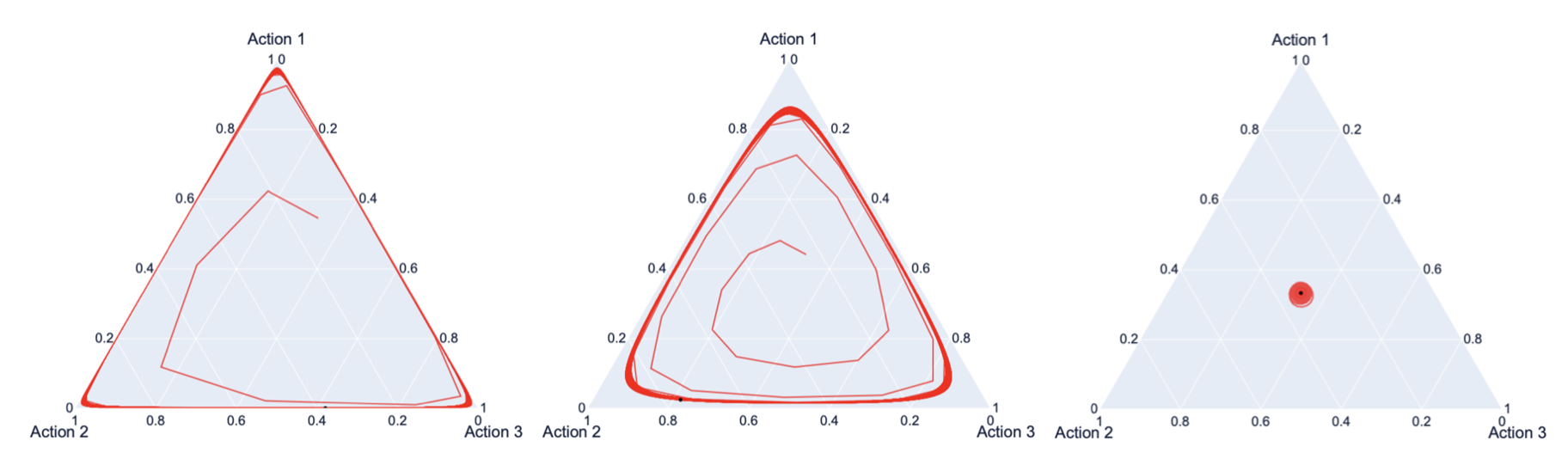
In the main paper, we consider the Network Sato Game, a multiplayer extension of the bimatrix game analysed in (Sato, Akiyama, and Farmer 2002). In the network variant, each edge defines the same bimatrix game , i.e. where
with . Notice that if , the game is zero-sum. In (Sato, Akiyama, and Farmer 2002; Sato and Crutchfield 2003) the case was analysed, and chaotic learning dynamics were found. In Figure 5, we plot trajectories generated by Q-Learning a seven agent network using a ring network and a fully connected network. We iterate Q-Learning for iterations and plot the mixed strategies of a single representative agent. In the ring network, it is clear that the dynamics do not converge for low choices of . In particular, for , Q-Learning displays the same chaotic behaviour shown in (Sato, Akiyama, and Farmer 2002) for the two-player case. At Q-Learning reaches the unique QRE at the uniform distribution . By contrast the fully connected network does not converge for but rather remains around the boundary of the simplex. Instead is required to reach the QRE.