Exact ASP Counting with Compact Encodings

Abstract

Answer Set Programming (ASP) has emerged as a promising paradigm in knowledge representation and automated reasoning owing to its ability to model hard combinatorial problems from diverse domains in a natural way. Building on advances in propositional SAT solving, the past two decades have witnessed the emergence of well-engineered systems for solving the answer set satisfiability problem, i.e., finding models or answer sets for a given answer set program. In recent years, there has been growing interest in problems beyond satisfiability, such as model counting, in the context of ASP. Akin to the early days of propositional model counting, state-of-the-art exact answer set counters do not scale well beyond small instances. Exact ASP counters struggle with handling larger input formulas. The primary contribution of this paper is a new ASP counting framework, called $\mathsf{sharpASP}$, which counts answer sets avoiding larger input formulas. This relies on an alternative way of defining answer sets that allows for the lifting of key techniques developed in the context of propositional model counting. Our extensive empirical analysis over $1470$ benchmarks demonstrates significant performance gain over current state-of-the-art exact answer set counters. Specifically, by using $\mathsf{sharpASP}$, we were able to solve $1062$ benchmarks with PAR2 score of $3082$ whereas using prior state-of-the-art, we could only solve $895$ benchmarks with a PAR2 score of $4205$, all other experimental conditions being the same.

1 Introduction

Answer Set Programming (ASP) (Marek and Truszczyński 1999) is a declarative problem-solving approach with a wide variety of applications ranging from planning, diagnosis, scheduling, and product configuration checking (Nouman et al. 2016; Brik and Remmel 2015; Tiihonen et al. 2003). An ASP program consists of a set of rules defined over propositional atoms, where each rule logically expresses an implication relation. An assignment to the propositional atoms satisfying the ASP semantic is called an answer set. In this paper, we focus on an important class of ASP programs called normal logic programs that have been used in diverse applications (see for example (Dodaro and Maratea 2017; Brooks et al. 2007)), and present a new technique to count answer sets of such programs, while scaling much beyond state-of-the-art exact answer set counters.

In general, given a set of constraints in a theory, model counting seeks to determine the number of models (or solutions) to the set of constraints. From a computational complexity perspective, this can be significantly harder than deciding whether there exists any solution to the set of constraints, i.e. the satisfiability problem. Yet, in the context of propositional reasoning, compelling applications have fuelled significant practical advances in propositional model counting, also referred to as #SAT (Sharma et al. 2019; Thurley 2006), over the past decade. This, in turn, has ushered in new applications in quantified information flow (Biondi et al. 2018), neural network verification (Baluta et al. 2019), computational biology, and the like. The success of practical propositional model counting in diverse application domains have naturally led researchers to ask if practically efficient counting algorithms can be devised for constraints beyond propositional logic. In particular, there has been growing interest in answer set counting, motivated by applications in probabilistic reasoning and network reliability (Kabir and Meel 2023).

Early efforts to build answer set counters sought to work by enumerating answer sets of a given ASP program (Fichte et al. 2017; Gebser et al. 2007). While this works extremely well for answer set counts upto a certain threshold, enumeration doesn’t scale well for problem instances with too many answer sets. Therefore, subsequent approaches to answer set counting sought to leverage the significant progress made in #SAT techniques. Specifically, Aziz et al. (Aziz et al. 2015) integrated a component-caching based propositional model counting technique with unfounded set detection to yield an answer set counter, called ASProblog. In another line of work, dynamic programming on a tree decomposition of the input problem instance has been proposed to achieve scalability for ASP instances with low treewidth (Fichte et al. 2017; Fichte and Hecher 2019). Yet another approach has been to translate a given normal logic program $P$ into a propositional formula $F$, such that there is a one-to-one correspondence between answer sets of $P$ and models of $F$ (Janhunen and Niemelä 2011; Bomanson 2017; Janhunen 2006). Answer sets of $P$ can then be counted by invoking an off-the-shelf propositional model counter (Sharma et al. 2019) on $F$. Though promising in principle, a naive application of this approach doesn’t scale well in practice owing to a blowup in the size of the resulting formula $F$ when the implications between propositional atoms encoded in the program $P$ give rise to circular dependencies (Lifschitz and Razborov 2006), which is a common occurrence when modeling numerous real-world applications. To address this, researchers have proposed techniques to transform the program to effectively break such circular dependencies and then use a treewidth-aware translation of the transformed program to a propositional formula (see, for example (Eiter, Hecher, and Kiesel 2021)). However, breaking such circular dependencies can increase the treewidth of the resulting transformed problem instance, which in turn can adversely affect the performance of answer set counting. Thus, despite significant advances, state-of-the-art exact answer set counters are stymied by scalability bottlenecks, limiting their practical applicability. Within this context, we ask the question: Can we design a scalable answer set counter, accompanied by a substantial reduction in the size of the transformed input program, particularly when addressing circular dependencies?

The principal contribution of this paper addresses the aforementioned question by introducing an alternative approach to exact answer set counting, called $\mathsf{sharpASP}$, while alleviating key bottlenecks faced by earlier approaches. While a mere reduction in translation size does not inherently establish a scalable ASP counting solution for general scenarios, $\mathsf{sharpASP}$ allows us to solve larger and more instances of exact answer set counting than was feasible earlier. Similar to ASProblog, $\mathsf{sharpASP}$ lifts component-caching based propositional model counting algorithms to ASP counting. The key idea that makes this possible is an alternative yet correlated perspective on defining answer sets. This alternative definition makes it possible to lift core ideas like decomposability and determinism in propositional model counters to facilitate answer set counting. Viewed differently, transforming propositional model counters into our proposed ASP counting framework requires minimal adjustments. Our experimental analysis demonstrates that $\mathsf{sharpASP}$, built using this approach, significantly outperforms the performance of previous state-of-the-art techniques across instances from diverse domains. This serves to underscore the effectiveness of our approach over the combined might of earlier state-of-the-art exact answer set counters.

The remainder of this paper is organized as follows. We present some preliminaries and notations in Section 2. Section 3 presents an alternative way of defining the answer set of an ASP instance, which allows us to propose the answer set counting algorithm of $\mathsf{sharpASP}$ in Section 4, where we also present correctness arguments for our algorithm. Section 5 presents our experimental evaluation of the proposed answer set counting algorithm. Finally, we conclude our paper in Section 6.

2 Preliminaries

Before delving into the details, we introduce some notation and preliminaries from propositional satisfiability and answer set programming.

Propositional Satisfiability.

A propositional variable $v$ takes one of two values: $0$ (denoting $\mathsf{false}$) or $1$ (denoting $\mathsf{true}$). A literal $\ell$ is either a variable (positive literal) or its negation (negated literal), and a clause $C$ is a disjunction of literals. For convenience of exposition, we sometimes represent a clause as a set of literals, with the implicit understanding that all literals in the set are disjoined in the clause. A clause with a single literal is also called a unit clause. In general, the constraint represented by a clause $C\equiv(\neg{v_{1}}\vee\ldots\vee\neg{v_{k}}\vee v_{k+1}\vee\ldots\vee v_{k+m})$ can be expressed as a logical implication: $(v_{1}\wedge\ldots\wedge v_{k})\rightarrow(v_{k+1}\vee\ldots\vee v_{k+m})$. If $k=0$, the antecedent of the above implication is $\mathsf{true}$, and if $m=0$, the consequent is $\mathsf{false}$. A conjunctive normal form (CNF) formula $\phi$ is a conjuction of clauses. When there is no confusion, a CNF formula is also sometimes represented as a set of clauses, with the implicit understanding that all clauses in the set are conjoined to give the formula. We denote the set of variables in $\phi$ as $\mathsf{Var}(\phi)$.

An assignment of a set $X$ of propositional variables is a mapping $\tau:X\rightarrow\{0,1\}$. For a variable $v\in X$, we define $\tau(\neg{v})=1-\tau(v)$. Given a CNF formula $\phi$ (as a set of clauses) and an assignment $\tau:X\rightarrow\{0,1\}$, where $X\subseteq\mathsf{Var}(\phi)$, the unit propagation of $\tau$ on $\phi$, denoted $\phi|_{\tau}$, is recursively defined as follows:

$\phi|_{\tau}=\begin{cases}1&\text{if $\phi\equiv 1$}\\ \phi^{\prime}|_{\tau}&\text{if $\exists C\in\phi$ s.t. $\phi^{\prime}=\phi\setminus\{C\}$,}\\ &\text{$\ell\in C$ and $\tau(\ell)=1$}\\ \phi^{\prime}|_{\tau}~{}\cup~{}\{C^{\prime}\}&\text{if $\exists C\in\phi$ s.t. $\phi^{\prime}=\phi^{\prime}\setminus\{C\}$,}\\ &\text{$\neg\ell\in C$,}\text{$C^{\prime}=C\setminus\{\neg\ell\}$}\\ &\text{ and ($\tau(\ell)=1$ or $\{l\}\in\phi$)}\end{cases}$

Note that $\phi|_{\tau}$ always reaches a fixpoint. We say that $\tau$ unit propagates to literal $\ell$ in $\phi$ if $\{\ell\}\in\phi|_{\tau}$, i.e. if $\phi|_{\tau}$ has a unit clause with the literal $\ell$.

Answer Set Programming.

An answer set program $P$ expresses logical constraints between a set of propositional variables. In the context of answer set programming, such variables are also called atoms, and the set of atoms appearing in $P$ is denoted $\mathsf{atoms}(P)$. For notational convenience, we will henceforth use the terms “variable” and “atom” interchangeably. A normal (logic) program is a set of rules of the following form:

$$\text{Rule $r$:~{}~{}}a\leftarrow b_{1},\ldots,b_{m},\sim c_{1},\ldots,\sim c_{n}$$ (1)

In the above rule, $\sim$ denotes default negation, signifying failure to prove (Clark 1978). For rule $r$ shown above, atom “$a$” is called the head of $r$ and is denoted $\mathsf{Head}(r)$. Similarly, the set of literals $\{b_{1},\ldots,b_{m},\sim c_{1},\ldots,\sim c_{n}\}$ is called the body of $r$. Specifically, $\{b_{1},\ldots,b_{m}\}$ are the positive body atoms, denoted $\mathsf{Body}(r)^{+}$, and $\{c_{1},\ldots,c_{n}\}$ are the negative body atoms, denoted $\mathsf{Body}(r)^{-}$. For purposes of the following discussion, we use $\mathsf{Body}(r)$ to denote the conjunction $b_{1}\wedge\ldots\wedge b_{m}\wedge\neg{c_{1}}\wedge\ldots\wedge\neg{c_{n}}$. Atoms that appear in the head of a rule (like $a$ in rule $r$ above) have also been called founded variables/atoms in the literature (Aziz et al. 2015).

In answer set programming, an interpretation $M\subseteq\mathsf{atoms}(P)$ lists the $\mathsf{true}$ atoms, i.e., an atom $a$ is $\mathsf{true}$ iff $a\in M$. An assignment $M$ satisfies $\mathsf{Body}(r)$, denoted $M\models\mathsf{Body}(r)$, iff $\mathsf{Body}(r)^{+}\subseteq M$ and $\mathsf{Body}(r)^{-}\cap M=\emptyset$, where $\sim$ is interpreted classically, i.e., $M\models\sim c_{i}$ iff $M\not\models c_{i}$. The rule $r$ (see Equation 1) specifies that if all atoms in $\mathsf{Body}(r)^{+}$ hold and no atom in $\mathsf{Body}(r)^{-}$ holds, then $\mathsf{Head}(r)$ also holds. The assignment $M$ satisfies rule $r$, denoted $M\models r$, if and only if whenever $M\models\mathsf{Body}(r)$, then $\mathsf{Head}(r)\in M$. Let $\mathsf{Rules}(P)$ denote the set of all rules in a normal program $P$. Then, we say that an assignment $M$ satisfies $P$, denoted $M\models P$, if and only if $M\models r$ for each $r\in\mathsf{Rules}(P)$.

Given an assignment (or set of atoms) $M$, the Gelfond-Lifschitz (GL) reduct of a program $P$ w.r.t. $M$ is defined as $P^{M}=\{\mathsf{Head}(r)\leftarrow\mathsf{Body}(r)^{+}~{}|~{}r\in\mathsf{Rules}(P),\mathsf{Body}(r)^{-}\cap M=\emptyset\}$ (Gelfond and Lifschitz 1988). A set of atoms $M$ is an answer set of $P$ if and only if $M\models P^{M}$, but $N\not\models P^{M}$ for every proper subset $N$ of $M$. The set of all answer sets of program $P$ is denoted by $\mathsf{AS}(P)$, and the answer set counting problem is to compute $|\mathsf{AS}(P)|$, which is denoted by $\mathsf{CntAS}(P)$.

Clark’s completion (Clark 1978) or program completion is a technique for obtaining a translation of a normal program $P$ into a related, but not semantically equivalent, propositional formula $\mathsf{Comp}(P)$. Specifically, for each atom $a\in\mathsf{atoms}(P)$, we do the following:

1. Let $r_{1},\ldots,r_{k}\in\mathsf{Rules}(P)$ such that $\mathsf{Head}(r_{1})=\ldots=\mathsf{Head}(r_{k})=a$, then we add the propositional formula $(a\leftrightarrow(\mathsf{Body}(r_{1})\vee\ldots\vee\mathsf{Body}(r_{k})))$ to $\mathsf{Comp}(P)$.

2. Otherwise, we add the literal $\neg{a}$ to $\mathsf{Comp}(P)$.

Finally, $\mathsf{Comp}(P)$ is obtained as the logical conjunction of all constraints added above. It has been shown in the literature that an answer set of $P$ satisfies $\mathsf{Comp}(P)$ but not vice versa (Lin and Zhao 2004).

To overcome the above problem, the idea of loop formula was introduced in (Lin and Zhao 2004). We outline the construction of a loop formula below. Given a normal program $P$, we start by defining the positive dependency graph $\mathsf{DG}(P)$ of $P$ as follows. The vertices of $\mathsf{DG}(P)$ are simply $\mathsf{atoms}(P)$. For $a,b\in\mathsf{atoms}(P)$, there exists an edge from $b$ to $a$ in $\mathsf{DG}(P)$ if there is a rule $r\in\mathsf{Rules}(P)$ such that $a\in\mathsf{Body}(r)$ and $b=\mathsf{Head}(r)$. A set of atoms $L\subseteq\mathsf{atoms}(P)$ constitutes a loop in $P$ if for every two atoms $x,y\in L$ there is a path from $x$ to $y$ in $\mathsf{DG}(P)$ such that all atoms (nodes) on the path are in $L$. An atom $a$ is called a loop atom of $P$ if there is a loop $L$ in $P$ such that $a\in L$. We use $\mathsf{Loops}(P)$ and $\mathsf{LA}(P)$ to denote the set of all loops and the set of all loop atoms of $P$, respectively. A program $P$ is called tight if there is no loop in $P$; otherwise, $P$ is called non-tight. Lin and Zhao (Lin and Zhao 2004) showed that atoms in a loop cannot be asserted $\mathsf{true}$ by themselves; instead they must be asserted by some atoms external to the loop. Specifically, a rule $r$ is an external support of a loop $L$ in $P$ if $\mathsf{Head}(r)\in L$ and $\mathsf{Body}(r)^{+}\cap L=\emptyset$. Let $\mathsf{ExtRule}(L)$ denote the set of all external supports of loop $L$ in $P$. The loop formula $\mathsf{LF}(L,P)$ (Lee and Lifschitz 2003) of a loop $L$ in program $P$ can now be defined as follows:

$$\mathsf{LF}(L,P) =\big{(}\bigwedge_{a\in L}a\big{)}\rightarrow\bigvee_{r\in\mathsf{ExtRule}(L)}\mathsf{Body}(r)$$

Finally, the loop formula $\mathsf{LF}(P)$ of program $P$ is defined as the conjunction of loop formulas for all loops $L$ in $P$, i.e. $\bigwedge_{L\in\mathsf{Loops}(P)}\mathsf{LF}(L,P)$. Let $M\subseteq\mathsf{atoms}(P)$ be a subset of atoms of $P$. We use $\tau^{M}:\mathsf{atoms}(P)\rightarrow\{0,1\}$ to denote the assignment corresponding to $M$, i.e. $\tau^{M}(v)=1$ if $v\in M$ and $\tau^{M}(v)=0$ otherwise, for all $v\in\mathsf{atoms}(P)$. Then $M$ is an answer set of $P$ if and only if $\tau^{M}$ satisfies the propositional formula $\mathsf{Comp}(P)\wedge\mathsf{LF}(P)$ (Lin and Zhao 2004).

2.1 Related Work

The decision version of normal logic programs is NP-complete; therefore, the ASP counting for normal logic programs is #P-complete (Valiant 1979). Given the #P-completeness, a prominent line of work focused on ASP counting relies on translations from the ASP program to the CNF formula (Lin and Zhao 2004; Janhunen 2004, 2006; Janhunen and Niemelä 2011). Such translations often result in a large number of CNF clauses and thereby limit practical scalability for non-tight ASP programs. Eiter et al. (2021) introduced T_P-unfolding to break cycles and produce a tight program. They proposed an ASP counter called aspmc, that performs a treewidth-aware Clark completion from a cycle-free program to the CNF formula. Jakl, Pichler, and Woltran (2009) extended the tree decomposition based approach for #SAT due to Samer and Szeider (2007) to Answer Set Programming and proposed a fixed-parameter tractable (FPT) algorithm for ASP counting. Fichte et al. (2017; 2019) revisited the FPT algorithm due to Jakl et al. and developed an exact model counter, called DynASP, that performs well on instances with low treewidth. Aziz et al. (2015) extended a propositional model counter to an answer set counter by integrating unfounded set detection. Kabir et al. (2022) focused on lifting hashing-based techniques to ASP counting, resulting in an approximate counter, called ApproxASP, with $(\varepsilon,\delta)$-guarantees.

3 An Alternative Definition of Answer Set

Our algorithm for answer set counting crucially relies on an alternative way of defining the answer sets of a normal program $P$. We first introduce an operation called $\mathsf{Copy}()$ that plays a central role in this alternative definition. Our $\mathsf{Copy}()$ operation is related to, but not the same as, a similar operation used in ASProblog. Specifically, founded variables (i.e. variables appearing at the head of a rule) were the focus of the copy operation used in ASProblog. In contrast, loop atoms in the program $P$ are the focus of the $\mathsf{Copy}()$ operation in our approach. We elaborate more on this below.

3.1 The Copy Operation

Given a normal program $P$, for every loop atom/variable $v$ in $\mathsf{LA}(P)$, let $v\textprime$ be a fresh variable not present in $\mathsf{atoms}(P)$. We refer to $v\textprime$ as the copy variable of $v$. For $X\subseteq\mathsf{LA}(P)$, we denote the set of copy variables corresponding to atoms in $X$ as $X\textprime$.

The $\mathsf{Copy}()$ operation, when applied to a normal program $P$, returns a set of (implicitly conjoined) implications, defined as follows:

1. (type 1) for every $v\in\mathsf{LA}(P)$, the implication $v\textprime\rightarrow v$ is in $\mathsf{Copy}(P)$.

2. (type 2) for every rule $x\leftarrow a_{1},\ldots a_{k},b_{1},\ldots b_{m},\sim c_{1},\ldots\sim c_{n}$ in $P$, where $x\in\mathsf{LA}(P)$, $\{a_{1},\ldots a_{k}\}\subseteq\mathsf{LA}(P)$ and $\{b_{1},\ldots b_{m}\}\cap\mathsf{LA}(P)=\emptyset$, the implication $a_{1}\textprime\wedge\ldots a_{k}\textprime\wedge b_{1}\wedge\ldots b_{m}\wedge\neg{c_{1}}\wedge\ldots\neg{c_{n}}\rightarrow x\textprime$ is in $\mathsf{Copy}(P)$.

3. No other implication is in $\mathsf{Copy}(P)$.

Note that in implications of type 2, copy variables are used exclusively for positive loop atoms in the body of the rule and for the loop atom in the head of the rule. Specifically, if the head of a rule is not a loop atom, we don’t add any implication of type 2 for that rule. As an extreme case, if $P$ is a tight program or $\mathsf{LA}(P)=\emptyset$, then $\mathsf{Copy}(P)$ is empty.

An Alternative Definition of Answer Set

We now present a key observation that provides the basis for an alternative definition of answer sets. Akin to the existing definitions of answer set (Janhunen 2006; Giunchiglia, Lierler, and Maratea 2006; Lifschitz 2010), our definition seeks justification for atoms within an answer set. However, our definition seeks to justify only loop atoms belonging to an answer set, while the existing definitions, to the best of our knowledge, aim to justify each atom in an answer set. The alternative definition derives from the observation that under Clark’s completion of a program, if the loop atoms of an answer set are justified, then the remaining atoms of the answer set are also justified. Thus, under Clark’s completion, it suffices to seek justifications for loop atoms. Unlike existing definitions of answer sets, our definition of answer sets operates exclusively within the realm of Boolean formulas and employs unit propagation as a tool to decide whether an atom is justified or not.

Recall from Section 2 the definition of $\phi|_{\tau}$, i.e. unit propagation of an assignment $\tau$ on a CNF formula $\phi$. Recall also that a CNF formula can be viewed as a set of clauses, where each clause can be interpreted as an implication. Therefore, the set of implications $\mathsf{Copy}(P)$ can be thought of as representing a CNF formula. For an assignment $\tau:X\rightarrow\{0,1\}$ where $X\subseteq\mathsf{atoms}(P)$, we use the notation $\mathsf{Copy}(P)|_{\tau}$ to denote the (implicitly conjoined) set of implications that remain after unit propagating $\tau$ on the CNF formula represented by $\mathsf{Copy}(P)$. Specifically, we say that $\mathsf{Copy}(P)|_{\tau}~{}=\emptyset$ if $\tau$ unit propagates to only unit clauses on copy variables in the CNF formula represented by $\mathsf{Copy}(P)$.

Theorem 1.

For a normal program $P$, let $X\subseteq\mathsf{atoms}(P)$ and let $\tau:X\mapsto\{0,1\}$ be an assignment. Let $M^{\tau}$ denote the set of atoms of $P$ that are assigned $1$ by $\tau$. Then $M^{\tau}\in\mathsf{AS}(P)$ if and only if $\tau\models\mathsf{Comp}(P)$ and $\mathsf{Copy}(P)|_{\tau}=\emptyset$.

Proof.

(i) (proof of ‘if part’) Proof By Contradiction. Assume that $\tau\models\mathsf{Comp}(P)$ and $\mathsf{Copy}(P)|_{\tau}=\emptyset$, but $M^{\tau}\not\in\mathsf{AS}(P)$. Since $M^{\tau}\not\in\mathsf{AS}(P)$ and $\tau\models\mathsf{Comp}(P)$, it implies that $\tau\not\models\mathsf{LF}(P)$. Thus, there is a loop $L$ in $P$ such that $\tau\not\models\mathsf{LF}(L,P)$. Assume that $L$ is comprised of the set of loop atoms $\{\,x_{1},\ldots,x_{k}\,\}$. Then $\tau\not\models x_{1}\wedge\ldots\wedge x_{k}\rightarrow\bigvee_{r\in\mathsf{ExtRule}(L)}\mathsf{Body}(r)$. In other words, even if $\tau$ is augmented by setting $x_{1}=\ldots=x_{k}=1$, the formula $\bigvee_{r\in\mathsf{ExtRule}(L)}\mathsf{Body}(r)$ evaluates to $0$ under the augmented assignment. Now recall that $\tau$ itself is an assignment to a subset of $\mathsf{atoms}(P)$, and it does not assign any truth value to $x_{1}\textprime,\ldots,x_{k}\textprime$. Therefore, there must be at least one type 2 implication in $\mathsf{Copy}(P)|_{\tau}$, specifically one arising from a rule $r\in\mathsf{ExtRule}(L)$, that does not unit propagate to a unit clause or to $1$ under $\tau$. This contradicts the premise that $\mathsf{Copy}(P)|_{\tau}=\emptyset$.

(ii) (proof of ‘only if part’) Proof By Contradiction. Suppose $M^{\tau}\in\mathsf{AS}(P)$. We know that this implies $\tau\models\mathsf{Comp}(P)\wedge\mathsf{LF}(P)$. We now show that in this case, we must also have $\mathsf{Copy}(P)|_{\tau}=\emptyset$. Suppose, if possible, $\mathsf{Copy}(P)|_{\tau}\neq\emptyset$. We ask if an implication of type 1, say $v\textprime\rightarrow v$, can stay back in $\mathsf{Copy}(P)|_{\tau}$. If $v\in M^{\tau}$, then $\tau(v)=1$, and clearly the implication $v\textprime\rightarrow v$ doesn’t stay back in $\mathsf{Copy}(P)|_{\tau}$. If $v\not\in M^{\tau}$, then $\tau(v)=0$, and in this case $\tau$ unit propagates to $\{\neg v\textprime\}$, and hence the implication doesn’t stay back in $\mathsf{Copy}(P)|_{\tau}$ either. Therefore, no implication of type 1 can stay back in $\mathsf{Copy}(P)|_{\tau}$. Next, we ask if any implication of type 2 can stay back in $\mathsf{Copy}(P)|_{\tau}$. Suppose this is possible. Note that for every $v\in\mathsf{atoms}(P)$, either $v\in M^{\tau}$ or $v\not\in M^{\tau}$. Therefore, $\tau(v)$ is either $0$ or $1$ for all $v\in\mathsf{atoms}(P)$. Therefore, if $\mathsf{Copy}(P)|_{\tau}\neq\emptyset$, there must be some $x_{1}\textprime\in\mathsf{Var}(\mathsf{Copy}(P)|_{\tau})$ and there must a (potentially simplified) implication $x_{2}\textprime\wedge C_{1}\rightarrow x_{1}\textprime$ in $\mathsf{Copy}(P)|_{\tau}$, where $C_{1}$ is either $\mathsf{true}$ or a conjunction of copy variables. The existence of copy variable $x_{2}\textprime$ in $\mathsf{Copy}(P)|_{\tau}$ implies the existence of another implication: $x_{3}\textprime\wedge C_{2}\rightarrow x_{2}\textprime$ in $\mathsf{Copy}(P)|_{\tau}$. Continuing this argument, we find that there are two cases to handle: (i) there are an unbounded number of copy variables in $\mathsf{Copy}(P)|_{\tau}$, which contradicts the fact that there can be at most $|\mathsf{Var}(P)|$ copy variables. (ii) otherwise, there exists $i,j$ such that $x_{i}\textprime=x_{j}\textprime$ and $i<j$, which implies that the set of variables $\{\,x_{i},\ldots x_{j-1}\,\}$ constitutes an unfounded set. However, this contradicts the fact that $M^{\tau}\in\mathsf{AS}(P)$. In either case, we reach a contradiction, thereby proving that $\mathsf{Copy}(P)|_{\tau}$ is empty. This completes the proof. ∎

Example 1.

Consider the normal program $P$ given by the rules $\{r_{1}=a\leftarrow\sim b.~{}\text{ }r_{2}=b\leftarrow\sim a.~{}\text{ }r_{3}=c\leftarrow a,b.\text{ }~{}r_{4}=c\leftarrow d.~{}\text{ }r_{5}=d\leftarrow a.~{}\text{ }r_{6}=d\leftarrow b,c.~{}\text{ }r_{7}=e\leftarrow\sim a,\sim b\}$.
This program has a single loop $L$ consisting of atoms $c$ and $d$, i.e. $\mathsf{LA}(P)=\{c,d\}$. Therefore, $\mathsf{Copy}(P)$ consists of the conjunction of implications: $\{\,c\textprime\rightarrow c,d\textprime\rightarrow d,a\wedge b\rightarrow c\textprime,d\textprime\rightarrow c\textprime,a\rightarrow d\textprime,b\wedge c\textprime\rightarrow d\textprime\,\}$. Note that there are no variables $a^{\prime},b^{\prime},e^{\prime}$ or constraints involving them in $\mathsf{Copy}(P)$. The followings are now easily verified.

• Consider $\tau_{1}$ that assigns $1$ to $b$ and $0$ to $a,c,d,e$. For the corresponding answer set $M^{\tau_{1}}$: $\{\,b\,\}$, $\mathsf{Copy}(P)|_{\tau_{1}}=\emptyset$

• Consider $\tau_{2}$ assigns $1$ to $a,c,d$ and $0$ to $b,e$. For the corresponding answer set $M^{\tau_{2}}$: $\{\,a,c,d\,\}$, $\mathsf{Copy}(P)|_{\tau_{2}}=\emptyset$

• Consider $\tau_{3}$ that assigns $1$ to $b,c,d$ and $0$ to $a,e$. For the corresponding non-answer set $M^{\tau_{3}}$: $\{\,b,c,d\,\}$, $\mathsf{Copy}(P)|_{\tau_{3}}\neq\emptyset$

4 Counting Answer Sets

In this section, we first show how the alternative definition of answer sets provides a new way to counting all answer sets of a given normal program. Subsequently, we explore how off-the-shelf state-of-the-art propositional model counters can be easily adapted to correctly count answer sets by leveraging the alternative definition.

It is easy to see from Theorem 1 that the count of answer sets of a normal program $P$ can be obtained simply by counting assignments $\tau\in 2^{|\mathsf{atoms}(P)|}$ such that $\tau\models\mathsf{Comp}(P)$ and $\mathsf{Copy}(P)|_{\tau}=\emptyset$. This motivates us to represent a normal program $P$ using a pair ($F$, $G$), where $F=\mathsf{Comp}(P)$ and $G=\mathsf{Copy}(P)$. Further, we discuss below how key ideas in state-of-the-art propositional model counters can be adapted to work with this pair representation of normal programs to yield exact answer set counters.

4.1 Decomposition

Propositional model counters often decompose the input CNF formula into disjoint subformulas to boost up the counting efficiency (Bayardo Jr and Pehoushek 2000) – for two formulas $\phi_{1}$ and $\phi_{2}$, if $\mathsf{Var}(\phi_{1})\cap\mathsf{Var}(\phi_{2})=\emptyset$, then $\phi_{1}$ and $\phi_{2}$ are decomposable, i.e., we can count the number of models of $\phi_{1}$ and $\phi_{2}$ separately and multiply these two counts to get the number of models of $\phi_{1}\wedge\phi_{2}$.

Given a normal program, our proposed definition involves a pair of formulas: $F$ and $G$. Specifically, we define component decomposition with respect to $(F,G)$ as follows:

Definition 1.

$(F_{1}\wedge F_{2},G_{1}\wedge G_{2})$ is decomposable to $(F_{1},G_{1})$ and $(F_{2},G_{2})$ if and only if $(\mathsf{Var}(F_{1})\cup\mathsf{Var}(G_{1}))\cap(\mathsf{Var}(F_{2})\cup\mathsf{Var}(G_{2}))=\emptyset$.

Finally, Proposition 1 offers evidence supporting the correctness of our proposed definition of decomposition in computing the number of answer sets.

Proposition 1.

Let $(F_{1}\wedge\ldots F_{k},G_{1}\wedge\ldots G_{k})$ is decomposed to $(F_{1},G_{1}),\ldots,(F_{k},G_{k})$ then $\mathsf{CntAS}(F_{1}\wedge\ldots F_{k},G_{1}\wedge\ldots G_{k})=\mathsf{CntAS}(F_{1},G_{1})\times\ldots\mathsf{CntAS}(F_{k},G_{k})$

Proof.

By definition of decomposition, we know that $\big{(}\mathsf{Var}(F_{i})\cup\mathsf{Var}(G_{i})\big{)}\cap\big{(}\mathsf{Var}(F_{j})\cup\mathsf{Var}(G_{j})\big{)}=\emptyset$ for $1\leq i<j\leq k$. This, in turn, implies that $\mathsf{Var}(G_{i})\cap\mathsf{Var}(G_{j})=\emptyset$ for $1\leq i<j\leq k$. Therefore, no variable (copy variable or otherwise) is common in $G_{i}$ and $G_{j}$, if $i\neq j$. Hence, for every assignment $\tau:\mathsf{atoms}(P)\rightarrow\{0,1\}$, unit propagation of $\tau$ on $G_{i}$ and $G_{j}$ must happen completely independent of each other, i.e. no unit literal obtained by unit propagation of $\tau$ on $G_{i}$ affects unit propagation of $\tau$ on $G_{j}$, and vice versa. In other words, $G_{i}|_{\tau}\wedge G_{j}|_{\tau}=(G_{i}\wedge G_{j})|_{\tau}$.

Let $F=F_{1}\wedge\ldots F_{k}$ and $G=G_{1}\wedge\ldots G_{k}$. In the following, we use the notation $\tau$ to denote an assignment $\mathsf{atoms}(P)\rightarrow\{0,1\}$, and $\tau_{i}$ to denote an assignment $\mathsf{atoms}(P)\cap(\mathsf{Var}(F_{i})\cup\mathsf{Var}(G_{i}))\rightarrow\{0,1\}$, for $1\leq i\leq k$. By virtue of the argument in the previous paragraph, it is easy to see that the domains of $\tau_{i}$ and $\tau_{j}$ are disjoint for $1\leq i<j\leq k$. We use the notation $\tau_{1}\cup\ldots\tau_{k}$ to denote the assignment $\mathsf{atoms}(P)\rightarrow\{0,1\}$ defined as follows: if $v\in\mathsf{atoms}(P)\cap\big{(}\mathsf{Var}(F_{i})\cup\mathsf{Var}(G_{i})\big{)}$, then $(\tau_{1}\cup\ldots\tau_{k})(v)=\tau_{i}(v)$. The proof now consists of showing the following two claims:

1. $\mathsf{CntAS}(F_{1},G_{1})\times\cdots\mathsf{CntAS}(F_{k},G_{k})\geq\mathsf{CntAS}(F,G)$.

2. $\mathsf{CntAS}(F_{1},G_{1})\times\cdots\mathsf{CntAS}(F_{k},G_{k})\leq\mathsf{CntAS}(F,G)$.

Proof of part 1: Suppose $\tau\in\mathsf{AS}(F,G)$. By definition, $\tau\models F$ and $G|_{\tau}=\emptyset$. Since $F=F_{1}\wedge\ldots F_{k}$, we know that $\tau\models F_{i}$ for $1\leq i\leq k$. By the above definition of $\tau_{i}$, it then follows that $\tau_{i}\models F_{i}$. Similarly, since unit propagation of $\tau$ on $G_{i}$ and $G_{j}$ happen independently for all $i\neq j$, and since unit propagation of $\tau$ on $G=G_{1}\wedge\ldots G_{k}$ gives $\emptyset$, we have $G_{i}|_{\tau_{i}}=\emptyset$ as well. It follows that $\tau_{i}\in\mathsf{AS}(F_{i},G_{i})$ for $1\leq i\leq k$. Therefore, every $\tau\in\mathsf{AS}(F,G)$ yields a sequence of $\tau_{i}\in\mathsf{AS}(F_{i},G_{i})$, for $1\leq i\leq k$. Since the domains of all $\tau_{i}$’s are distinct, it follows that $\mathsf{CntAS}(F_{1},G_{1})\times\cdots\mathsf{CntAS}(F_{k},G_{k})\geq\mathsf{CntAS}(F,G)$.

Proof of part 2: Suppose $\tau_{i}\in\mathsf{AS}(F_{i},G_{i})$ for $1\leq i\leq k$. By definition, $\tau_{i}\models F_{i}$ and $G_{i}|_{\tau_{i}}=\emptyset$. Since the domains of $\tau_{i}$ and $\tau_{j}$ are disjoint for all $1\leq i<j\leq k$, it follows that $(\tau_{1}\cup\ldots\tau_{k})\models(F_{1}\wedge\ldots F_{k})$ and hence $\tau\models F$. We have also seen that $(G_{1}\wedge\cdots G_{k})|_{\tau}=(G_{1}|_{\tau}\wedge\cdots G_{k}|_{\tau})$. However, since $\mathsf{Var}(G_{i})$ is a subset of the domain of $\tau_{i}$, we have $(G_{1}\wedge\cdots G_{k})|_{\tau}=(G_{1}|_{\tau_{1}}\wedge\cdots G_{k}|_{\tau_{k}})$. Since $G_{i}|_{\tau_{i}}=\emptyset$ for $1\leq i\leq k$, it follows that $(G_{1}\wedge\cdots G_{k})|_{\tau}=\emptyset$. Therefore $G|_{\tau}=\emptyset$. Since $\tau\models F$ as well, we have $\tau\in\mathsf{AS}(F,G)$. Therefore, every distinct sequence of $\tau_{i},1\leq i\leq k$ such that $\tau_{i}\in\mathsf{AS}(F_{i},G_{i})$ yields a distinct $\tau\in\mathsf{AS}(F,G)$. It follows that $\mathsf{CntAS}(F_{1},G_{1})\times\cdots\mathsf{CntAS}(F_{k},G_{k})\leq\mathsf{CntAS}(F,G)$.

It follows from the above two claims that

$$\mathsf{CntAS}(F_{1},G_{1})\times\cdots\mathsf{CntAS}(F_{k},G_{k})=\mathsf{CntAS}(F,G).$$

∎

One of the drawbacks of the definition is its comparative weakness in relation to the conventional definition of decomposition. When dealing with a hard-to-decompose program $(F,G)$, then the process of counting answer sets regresses to enumerating the answer sets of the program.

4.2 Determinism

Propositional model counters utilize determinism (Darwiche 2002), which involves assigning one of the variables in a formula to either $\mathsf{false}$ or $\mathsf{true}$. The number of models of $\phi$ is then determined as the sum of the number of models in which a variable $x\in\mathsf{Var}(\phi)$ is assigned to $\mathsf{false}$ and $\mathsf{true}$. A similar idea can be used for answer set counting using our pair representation as well. To establish the correctness of the determinism employed in our approach, we first introduce two helper propositions: Proposition 2 and 3.

Proposition 2.

For partial assignment $\tau$ and program $P$ represented as $(\mathsf{Comp}(P),\mathsf{Copy}(P))$, if $\mathsf{Comp}(P)|_{\tau}=\emptyset$ and $\emptyset\subset\mathsf{Var}(\mathsf{Copy}(P)|_{\tau})\subseteq\mathsf{CopyVar}(P)$, then $\exists L\in\mathsf{Loops}(P)$ s.t. $L\subseteq M^{\tau}$ and $\tau\not\models\mathsf{LF}(L,P)$.

Proof.

Since $\emptyset\subset\mathsf{Var}(\mathsf{Copy}(P)|_{\tau})\subseteq\mathsf{CopyVar}(P)$, there exists a copy variable $x_{i_{1}}\textprime\in\mathsf{Var}(\mathsf{Copy}(P)|_{\tau})$ and an implication (simplified after unit propagation) of type 2 of the form $C_{1}\rightarrow x_{i_{1}}\textprime$ in $\mathsf{Copy}(P)|_{\tau}$, where $C_{1}$ is a non-empty conjunction of copy variables. Let $x_{i_{2}}\textprime\in\mathsf{Var}(C_{1})$, then there must also exist another implication (simplified after unit propagation) $C_{2}\rightarrow x_{i_{2}}\textprime$ in $\mathsf{Copy}(P)|_{\tau}$, where $C_{2}$ is again a conjunction of copy variables. Accordingly, for $x_{i_{3}}\in\mathsf{Var}(C_{2})\setminus\mathsf{Var}(C_{1})$, we have another implication of the form $C_{3}\rightarrow x_{i_{3}}\textprime$ in $\mathsf{Copy}(P)|_{\tau}$. Since the number of atoms is bounded, it must be the case that there exists $i_{k}$ such that there is an implication (simplified) of type 2 $C_{k}\rightarrow x_{k}\textprime$ such that $C_{k}\setminus(C_{1}\cup C_{2}\ldots C_{k-1})=\emptyset$.

Now, observation $C_{k}\setminus(C_{1}\cup C_{2}\ldots C_{k-1})=\emptyset$ implies existence of an atom set $L=\{x_{i_{1}},x_{i_{2}},\ldots x_{i_{j}}\}\subseteq\{x_{i_{1}},x_{i_{2}},\ldots x_{i_{k}}\}$ that forms a loop in $\mathsf{DG}(P)$. Given that $\mathsf{Var}(\mathsf{Copy}(P)|_{\tau})\subseteq\mathsf{CopyVar}(P)$, we also know that $\tau$ assigns a value to every $x\in\mathsf{Var}(\mathsf{Copy}(P))\cap\mathsf{atoms}(P)$. Furthermore, each of the atoms $x_{i_{1}},\ldots x_{i_{k}}$ must have been assigned $1$ by $\tau$. Otherwise, if any $x_{i_{l}}$ was assigned $0$ by $\tau$, then $\tau$ would have unit propagated on $\mathsf{Copy}(P)|_{\tau}$ to $\neg x_{i_{l}}^{\prime}$, which contradicts the observation that the copy variables $x_{i_{1}}^{\prime},\ldots x_{i_{k}}^{\prime}$ stayed backed in antecedents of implications of type 2 in $\mathsf{Copy}(P)|_{\tau}$. It follows that atoms in loop $L$ form a subset of atoms assigned $1$ by $\tau$.

We have shown above that $\{x_{i_{1}},x_{i_{2}},\ldots x_{i_{j}}\}$ constitutes a loop in the positive dependency graph. We now show by contradiction that $\tau\not\models\bigvee_{r\in\mathsf{ExtRule}(L)}\mathsf{Body}(r)$. Indeed, if $\tau\models\bigvee_{r\in\mathsf{ExtRule}(L)}\mathsf{Body}(r)$, let $x_{i_{t}}$ be $\mathsf{Head}(r)$ for a rule $r$ such that $\tau\models\mathsf{Body}(r)$. In this case, $\tau$ must have unit propagated to $\{x_{i_{t}}^{\prime}\}$ in $\mathsf{Copy}(P)|_{\tau}$. This contradicts the fact that the copy variables $x_{i_{1}}^{\prime},\ldots x_{i_{k}}^{\prime}$ stayed backed in antecedents of implications of type 2 in $\mathsf{Copy}(P)|_{\tau}$.

Therefore $\tau\models x_{i_{1}}\wedge\ldots x_{i_{j}}$ but $\tau\not\models\bigvee_{r\in\mathsf{ExtRule}(L)}\mathsf{Body}(r)$. This shows that $\tau\not\models\mathsf{LF}(L,P)$. ∎

Proposition 3.

For partial assignment $\tau$ and program $P$ represented as $(\mathsf{Comp}(P),\mathsf{Copy}(P))$, suppose $\tau\not\models\mathsf{LF}(L,P)$, where $L=\{x_{1},\ldots,x_{k}\}$. Then there exists $\tau^{+}$ such that $\{x_{1}\textprime,\ldots,x_{k}\textprime\}\subseteq\mathsf{Var}(\mathsf{Copy}(P)|_{\tau^{+}})$, $\mathsf{Comp}(P)|_{\tau^{+}}=\emptyset$ and $\tau\subseteq\tau^{+}$.

Proof.

As $\tau\not\models\mathsf{LF}(L,P)$, we have $\forall x_{i}\in L,\tau(x_{i})=1$ and $\forall r\in\mathsf{ExtRule}(L),\tau\not\models\mathsf{Body}(r)$. Let us denote by $r^{\prime}$ an implication of type 2 corresponding to a rule $r\in\mathsf{ExtRule}(L)$. Then we have $r^{\prime}|_{\tau}\neq\emptyset$; moreover, if $\mathsf{Head}(r)=x_{i}$, then $x_{i}\textprime\in\mathsf{Var}(r|_{\tau})$. Since the above observation holds for all $r\in\mathsf{ExtRule}(L)$ and for $x_{i}\in L$, therefore, $\{x_{1}\textprime,\ldots,x_{k}\textprime\}\subseteq\mathsf{Var}(\mathsf{Copy}(P)|_{\tau})$. Observe that for every extension $\tau^{\prime}$ of $\tau$ that does not assign values to variables in $\{x_{1}\textprime,\ldots,x_{k}\textprime\}$, it must be the case that $\{x_{1}\textprime,\ldots,x_{k}\textprime\}\subseteq\mathsf{Var}(\mathsf{Copy}(P)|_{\tau^{\prime}})$. Furthermore, since the set of variables in $\mathsf{Comp}(P)$ does not contain a variable from the set $\{x_{1}\textprime,\ldots,x_{k}\textprime\}$, therefore, there exists an extension, $\tau^{+}$, of $\tau$ such that $\mathsf{Comp}(P)|_{\tau^{+}}=\emptyset$ and $\{x_{1}\textprime,\ldots,x_{k}\textprime\}\subseteq\mathsf{Var}(\mathsf{Copy}(P)|_{\tau^{\prime}})$. ∎

We are now ready to state and prove the correctness of determinism employed in our ASP counter:

Proposition 4.

Let program $P$ be represented as $(F,G)$. Then

$$\mathsf{CntAS}(F,G) =\mathsf{CntAS}(F|_{\neg{x}},G|_{\neg{x}})+\mathsf{CntAS}(F|_{x},G|_{x}),$$

$$~{}~{}\text{for all }x\in\mathsf{atoms}(P)$$ (2)

$$\mathsf{CntAS}(\bot,G) =0$$ (3)

$$\mathsf{CntAS}(\emptyset,G) =\begin{cases}1&\text{if $G=\emptyset$ }\\ 0&\text{if $\mathsf{Var}(G)\subseteq\mathsf{CopyVar}(P)$ }\end{cases}$$ (4)

Note that if $\mathsf{Comp}(P)=\emptyset$ then either $G=\emptyset$ or $\emptyset\subset\mathsf{Var}(G)\subseteq\mathsf{CopyVar}(P)$.

Proof.

The proof comprises the following three parts:

Equation 2 applies determinism by partitioning all answer sets of $(F,G)$ into two parts – the answer sets where $x$ is $0$ and $1$, respectively. Observe that performing unit propagation on $(F,G)$ is valid since $\tau\in\mathsf{AS}(F|_{\sigma},G|_{\sigma})$ if and only if $\sigma\cup\tau\in\mathsf{AS}(F,G)$, where $\sigma\in 2^{|X|}$, $\tau\in 2^{|\mathsf{atoms}(P)\setminus X|}$, where $X\subseteq\mathsf{atoms}(P)$.

The proof of the first base case eq. 3 is trivial. Each answer set of $P$ conforms to the completion of the program $\mathsf{Comp}(P)$, where, according to the alternative definition of answer sets, $F=\mathsf{Comp}(P)$.

We utilize the helper propositions proved earlier to demonstrate the correctness of the second base case, as outlined in eq. 4, which appropriately selects answer sets from the models of completion. First, we show that if there is a copy variable in $\mathsf{Copy}(P)|_{\tau}$, where $\mathsf{Comp}(P)|_{\tau}=\emptyset$, then one of the loop formulas of the program is not satisfied by $\tau$. The claim is proved in Proposition 2. Thus, $\tau$ cannot be extended to an answer set. Second, we demonstrate that if there is an unsatisfied loop formula under a partial assignment $\tau_{1}$, then there exists $\tau_{1}^{+}$ such that some copy variables are not propagated in $\mathsf{Copy}(P)|_{\tau_{1}^{+}}$, where $\mathsf{Comp}(P)|_{\tau_{1}^{+}}=\emptyset$ and $\tau_{1}\subseteq\tau_{1}^{+}$. The claim is established in Proposition 3. Thus, through the method of contradiction, we can infer that, for an assignment $\tau$, if $\mathsf{Copy}(P)|_{\tau}=\emptyset$, then $\tau$ can be extended to an answer set.

∎

4.3 Conjoin $F$ and $G$

Until now, we have represented a program $P$ as a pair of formulas $F$ and $G$. However, in this subsection, we illustrate that rather than considering the pair, we can regard their conjunction $F\wedge G$, and all the subroutines of model counting algorithms work correctly. First, in Proposition 5, we demonstrate that $F\wedge G$ uniquely defines a program $(F,G)$ under arbitrary partial assignments.

Proposition 5.

For two assignments $\tau_{1}$ and $\tau_{2}$, and given a normal program, $F|_{\tau_{1}}\wedge G|_{\tau_{1}}=F|_{\tau_{2}}\wedge G|_{\tau_{2}}$ if and only if $F|_{\tau_{1}}=F|_{\tau_{2}}$ and $G|_{\tau_{1}}=G|_{\tau_{2}}$

Proof.

(i) (proof of ‘if part’) The proof is trivial.

(ii) (proof of ‘only if part’) Proof By Contradiction. Assume that there is a clause $c\in F|_{\tau_{1}}$ and $c\not\in F|_{\tau_{2}}$. As $F|_{\tau_{1}}\wedge G|_{\tau_{1}}=F|_{\tau_{2}}\wedge G|_{\tau_{2}}$ clause $c\in G|_{\tau_{2}}$. As $c\in F|_{\tau_{1}}$, $c$ has no copy variable. Assume that clause $c$ is derived from the unit propagation of $\mathsf{Copy}(r)$, i.e., $c=\mathsf{Copy}(r)|_{\tau_{2}}=a_{1}\textprime\wedge\ldots\wedge a_{k}\textprime\wedge b_{1}\wedge\ldots\wedge b_{m}\wedge\neg{c_{1}}\wedge\ldots\wedge\neg{c_{n}}\rightarrow x\textprime|_{\tau_{2}}$, where $\forall i,a_{i}\textprime$ propagates to $1$ and $x\textprime$ propagates to $0$, which follows that under assignment $\tau_{2}$, the atom $x$ is assigned to $0$ and $\forall i,a_{i}$ is assigned to $1$. The rule $r$ also belongs to $\mathsf{Comp}(P)$ and both $F|_{\tau_{1}}$ and $F|_{\tau_{2}}$ are derived from $\mathsf{Comp}(P)$. Thus, under assignment $\tau_{2}$, if $x$ is assigned to $0$ and each of the $a_{i}$’s is assigned to $1$, then the clause $c\in F|_{\tau_{2}}$, which must be derived from rule $r$, so contradiction. ∎

As a result, it is possible to perform unit propagation on $F\wedge G$ instead of performing unit propagation on $F$ and $G$ separately. Although both formulas $F$ and $G$ are necessary to check the base cases, we can still check base cases by considering the conjunction $F\wedge G$. Checking the first base case (eq. 3) is trivial because if an assignment $\tau$ conflicts on $F$, then $\tau$ conflicts on $F\wedge G$ as well. Additionally, calculating $\mathsf{Var}(F\wedge G)$ suffices to check the second base case (eq. 4). The component decomposition part also works with their conjunction because the component decomposition condition $(\mathsf{Var}(F_{1})\cup\mathsf{Var}(G_{1}))\cap(\mathsf{Var}(F_{2})\cup\mathsf{Var}(G_{2}))=\emptyset$ is equivalent to $(\mathsf{Var}(F_{1}\wedge G_{1}))\cap(\mathsf{Var}(F_{2}\wedge G_{2}))=\emptyset$. Moreover, as we restrict our decision to $\mathsf{atoms}(P)$, the conjunction $F\wedge G$ does not introduce new conflicts — if a partial assignment $\tau$ conflicts on $F\wedge G$, then $\tau$ conflicts on $F$. To summarize, the model counting algorithm correctly computes the answer set count, even when processing the formula $F\wedge G$ instead of processing the two formulas $F$ and $G$ separately.

4.4 $\mathsf{sharpASP}$: Putting It All Together

In this subsection, we aim to extend a propositional model counter to an exact answer set counter by integrating the alternative answer set definition, component decomposition (Proposition 1), and determinism (Equation 2).

Algorithm 1 $\mathsf{sharpASP}(P)$

1:function $\mathsf{Counter}(\phi,CV)$ $\triangleright$ modified CNF counter

2:     if $\phi=\emptyset$ then return $1$

3:     else if $\mathsf{Var}(\phi)\subseteq CV$ then return $0$

4:     else if $\emptyset\in\phi$ then return $0$      

5:     $\mathsf{v}\leftarrow\mathsf{PickNonCopyVar}(\phi)$

6:     for $\ell\leftarrow\{\mathsf{v},\neg{\mathsf{v}}\}$ do

7:         $\mathsf{Count}[\ell]\leftarrow 1$

8:         $\mathsf{comps}\leftarrow\mathsf{Decomposition}(\phi|_{\ell})$

9:         for each $\mathsf{c}\in\mathsf{comps}$ do

10:              if $\mathsf{c}\in\mathsf{Cache}$ then

11:                  $\mathsf{Count}[\ell]\leftarrow\mathsf{Count}[\ell]\times\mathsf{Cache}[\mathsf{c}]$

12:              else

13:                  $\mathsf{Count}[\ell]\leftarrow\mathsf{Count}[\ell]\times\mathsf{Counter}(\mathsf{c},CV)$               

14:              if $\mathsf{Count}[\ell]=0$ then

15:                  break                             

16:     $\mathsf{Cache}[\phi]\leftarrow\mathsf{Count}[\mathsf{v}]+\mathsf{Count}[\neg{\mathsf{v}}]$

17:     return $\mathsf{Cache}[\phi]$

18:end function

19:$F\leftarrow\mathsf{Comp}(P),G\leftarrow\mathsf{Copy}(P)$ $\triangleright$ Algorithm starts here

20:return $\mathsf{Counter}(F\wedge G,\mathsf{CopyVar}(P))$

The pseudocode for $\mathsf{sharpASP}$ is presented in Algorithm 1. Given a non-tight program $P$, $\mathsf{sharpASP}$ initially computes $\mathsf{Comp}(P)$ and $\mathsf{Copy}(P)$ (Line 19 of Algorithm 1) and then calls the adapted propositional model counter $\mathsf{Counter}$, with $\mathsf{Comp}(P)\wedge\mathsf{Copy}(P)$ as the input formula, and $\mathsf{CopyVar}(P)$ as the set of copy variables (Line 20 of Algorithm 1). The model counting algorithm utilizes $\mathsf{CopyVar}(P)$ to check the base cases (Equation (3) and (4)) of the Equation 2.

The $\mathsf{Counter}$ differs from the existing propositional model counters mainly in two ways. Firstly, following eq. 4, the $\mathsf{Counter}$ returns $0$ if it encounters a component consisting solely of copy variables (Line 3 of Algorithm 1). Secondly, during variable branching, $\mathsf{Counter}$ selects variables from $\mathsf{Var}(\mathsf{Comp}(P))$ (Line 5 of Algorithm 1). Apart from that, the subroutines of unit propagation, component decomposition (Line 8 of Algorithm 1), and caching (Line 10 of Algorithm 1) within $\mathsf{Counter}$ and a propositional model counter remain unchanged.

While $\mathsf{sharpASP}$ uses copy variables and copy operations similar to ASProblog, there are notable distinctions between the two approaches. Firstly, $\mathsf{sharpASP}$ aims to justify only loop atoms, whereas the ASProblog algorithm aims to justify all founded variables. Our empirical findings underscore that loop atoms constitute a relatively small subset of the founded variables. Consequently, the copy operation of ASProblog introduces more copy variables and logical implications involving copy variables compared to ours. Secondly, the unit propagation techniques employed in ASProblog differ from those used in $\mathsf{sharpASP}$. Specifically, ASProblog  performs unit propagation by propagating only the justified literals from a program while leaving the unjustified literals in the residual program. In contrast, $\mathsf{sharpASP}$ adheres to the conventional unit propagation technique and employs copy variables to determine whether all atoms are justified.

5 Experimental Evaluation

We developed a prototype of $\mathsf{sharpASP}$ on top of the existing state-of-the-art model counters (GANAK, D4, and SharpSAT-TD) (Korhonen and Järvisalo 2021; Sharma et al. 2019; Lagniez and Marquis 2017). We modified SharpSAT-TD by disabling all the preprocessing techniques, as they would no longer preserve answer sets. We use notations $\mathsf{sharpASP}$(STD), $\mathsf{sharpASP}$(G), and $\mathsf{sharpASP}$(D) to represent $\mathsf{sharpASP}$ with underlying propositional model counters SharpSAT-TD, GANAK, and D4, respectively.

We compared the performance of $\mathsf{sharpASP}$ with that of the prior state-of-the-art exact ASP counters: clingo  (Gebser et al. 2007), ASProblog (Aziz et al. 2015), and DynASP (Fichte et al. 2017). In addition, we utilized two translations from ASP to SAT: (i) lp2sat (Fages 1994; Janhunen and Niemelä 2011; Bomanson 2017)  (ii) aspmc (Eiter, Hecher, and Kiesel 2021), followed by invoking off-the-shelf propositional model counters. We use notations lp2sat+X and aspmc+X to denote lp2sat and aspmc followed by propositional model counter X, respectively.

Our benchmark suite consists of non-tight programs from the domains of the Hamiltonian cycle and graph reachability problems (Kabir et al. 2022; Aziz et al. 2015). We also considered the benchmark set from (Eiter, Hecher, and Kiesel 2021) (designated as aspben). We gathered a total of $1470$ graph instances from the benchmark set of (Kabir et al. 2022; Eiter, Hecher, and Kiesel 2021). The choice/random variables in the hamiltonian cycle and aspmc benchmark pertain to graph edges. While the choice variables are associated with graph nodes for the graph reachability problem.

All experiments were carried out on a high-performance computer cluster, where each node consists of AMD EPYC $7713$ CPUs running with $128$ real cores. The runtime and memory limit were set to $5000$ seconds and $8$GB, respectively.

5.1 Runtime Performance Comparison

				aspmc			lp2sat			$\mathsf{sharpASP}$
	clingo	ASProb	DynASP	D	G	STD	D	G	STD	D	G	STD
Hamil. (405)	230	0	0	173	197	167	135	164	112	238	261	300
Reach. (600)	318	149	2	187	288	421	317	471	167	293	458	463
aspben (465)	321	39	208	278	285	252	278	193	193	282	273	260
Total (1470)	869 (4285)	188 (8722)	210 (8571)	638 (5829)	770 (5015)	840 (4572)	730 (5282)	668 (5734)	776 (5082)	813 (4514)	992 (3473)	1023 (3372)

Table 1: The performance comparison of $\mathsf{sharpASP}$ vis-a-vis other ASP counters on different problems in terms of number of solved instances and PAR$2$ scores.

		clingo ($\leq 10^{5}$) +
	clingo	ASProb	aspmc +STD	lp2sat +STD	$\mathsf{sharpASP}$ (STD)
Hamil. (405)	230	123	167	128	302
Reach. (600)	318	152	418	470	460
aspben (465)	321	278	284	297	300
Total (1470)	869 (4285)	553 (6239)	869 (4310)	895 (4205)	1062 (3082)

Table 2: The performance comparison of hybrid counters in terms of number of solved instances and PAR$2$ scores. The hybrid counters correspond to last $4$ columns that employ clingo enumeration followed by ASP counters. The clingo ($2$nd column) refers to clingo enumeration for $5000$ seconds.

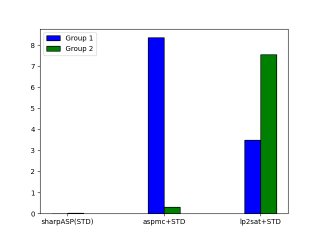
(a) Time spent in BCP (seconds)

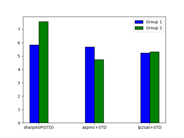
(b) Number of decisions ($10$-base log).

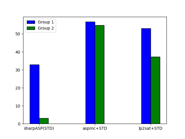
(c) Cache hit (percentage).

Figure 1: The ablation study of $\mathsf{sharpASP}$(STD), lp2sat+STD, and aspmc+STD on Group $1$ and Group $2$ benchmarks.

The performance of our considered counters varies across different computational problems. Our evaluation of their performance, considering both total solved instances and PAR$2$ scores, for each computational problem is detailed in Table 1. The table demonstrates that $\mathsf{sharpASP}$ either outperforms or achieves performance on par with existing ASP counters, particularly for the Hamiltonian cycle and graph reachability problems. However, on aspben, the clingo enumeration outperforms other answer set counters.

We observed that clingo demonstrates superior performance, particularly on instances with a limited number of answer sets. Since this observation applies to all non-enumeration based counters in our repertoire, we devised a hybrid counter that combines the strengths of enumeration based counting with that of translation and propositional SAT based counting. Based on data collected from runs of clingo, there is a shift in the runtime performance of clingo when the count of answer sets exceeds $10^{5}$ (within our benchmarks). To ensure that our experiments can be replicated on different platforms, we chose to use an answer set count-based threshold instead of a time-based threshold. Hence, our hybrid counter is structured as follows: it initiates enumeration with a maximum of $10^{5}$ answer sets. In cases where not all answer sets are enumerated, the hybrid counter then employs an ASP counter with a time limit of $5000-t$ seconds, where $t$ is the time spent in clingo. The performance of the hybrid counters is tabulated in Table 2, demonstrating that the hybrid counter based on $\mathsf{sharpASP}$ clearly outperforms competitors by a handsome margin.

5.2 Ablation Study

We now delve into the internals, and to this end, we form two groups of benchmarks – Group $1$: instances where $\mathsf{sharpASP}$(STD) runs faster than lp2sat+STD and aspmc+STD, which highlights the scenarios where the $\mathsf{sharpASP}$(STD) algorithm is more efficient than lp2sat+STD and aspmc+STD; and Group $2$: instances where lp2sat+STD and aspmc+STD run faster than $\mathsf{sharpASP}$(STD), which shows the opposite scenario of Group $1$. Each group consists of $10$ instances that had more than $10^{5}$ answer sets, and therefore clingo could not enumerate all answer sets. By running the instances on all versions of SharpSAT-TD, we record the time spent on the procedure binary constraint propagation (BCP), number of decisions, and cache hit rate for each counter. Taking each group’s average of each quantity provides a clear and concise way to see how $\mathsf{sharpASP}$ compares with others on average across all benchmarks. The statistical findings across all counters are visually summarized in Figure 1.

The strength of $\mathsf{sharpASP}$ lies in its ability to minimize the time spent on binary constraint propagation (BCP) compared to other counters. The significantly large formula size increases the overhead for BCP in the case of lp2sat+STD and aspmc+STD. However, we also observe that $\mathsf{sharpASP}$ suffers from high overhead in the branching phase and high cache misses on Group $2$ instances. To find out the reason for a higher number of decisions, we analyze the decomposibility of Group $1$ and Group $2$ instances.

Our investigation has shown that, on all variants of SharpSAT-TD, most instances of Group $1$ start decomposing at nearly the same decision levels. Thus, $\mathsf{sharpASP}$(STD) outperforms on Group $1$ instances due to spending less time on BCP. We observed that several instances of Group $1$ took comparatively more decisions to make to count the number of answer sets on $\mathsf{sharpASP}$(STD). One possible explanation is that aspmc+STD and lp2sat+STD assign auxiliary variables, which have higher activity scores compared to original ASP program variables. Assigning auxiliary variables facilitates lp2sat+STD and aspmc+STD by assigning fewer variables. However, $\mathsf{sharpASP}$(STD) outperforms others due to structural simplicity and low-cost BCP.

Our investigation has also revealed that Group $2$ instances are hard-to-decompose on $\mathsf{sharpASP}$(STD) compared to other counters – necessitating more variable assignments to break down an instance into disjoint components. Since $\mathsf{sharpASP}$(STD) assigns the original set of variables; it necessitates a larger number of decisions to count answer sets on hard-to-decompose instances compared to aspmc and lp2sat based counters. Moreover, the structure of hard-to-decompose instances also worsens the cache performance of $\mathsf{sharpASP}$. However, lp2sat+STD and aspmc+STD effectively decompose the input formula by initially assigning auxiliary variables.

In light of these findings, it is evident that the performance of $\mathsf{sharpASP}$ is critically reliant on the decomposability of input instances and the variable branching heuristic employed. Notably, $\mathsf{sharpASP}$ demonstrates superior performance when applied to structurally simpler input instances. If a variable branching heuristic effectively decomposes the input formula by assigning variables within the ASP programs, $\mathsf{sharpASP}$ outperforms alternative ASP counters. Conversely, when the input formula’s decomposability is hindered, alternative approaches involving the introduction of auxiliary variables prove to be more advantageous.

6 Conclusion

Our approach, called $\mathsf{sharpASP}$, lifts the component caching-based propositional model counting to ASP counting without incurring a blowup in the size of the resulting formula. The proposed approach utilizes an alternative definition for answer sets, which enables the natural lifting of decomposability and determinism. Empirical evaluations show that $\mathsf{sharpASP}$ and its corresponding hybrid solver can handle a greater number of instances compared to other techniques. As a future avenue of research, we plan to investigate extensions of our approach in the context of disjunctive programs.

Acknowledgement

This work was supported in part by National Research Foundation Singapore under its NRF Fellowship Programme [NRF-NRFFAI1-2019-0004], Ministry of Education Singapore Tier $2$ grant MOE-T2EP20121-0011, and Ministry of Education Singapore Tier $1$ Grant [R-252-000-B59-114]. The computational work for this article was performed on resources of the National Supercomputing Centre, Singapore (https://www.nscc.sg).

References

- Aziz et al. (2015) Aziz, R. A.; Chu, G.; Muise, C.; and Stuckey, P. J. 2015. Stable model counting and its application in probabilistic logic programming. In AAAI.
- Baluta et al. (2019) Baluta, T.; Shen, S.; Shinde, S.; Meel, K. S.; and Saxena, P. 2019. Quantitative verification of neural networks and its security applications. In Proceedings of the 2019 ACM SIGSAC Conference on Computer and Communications Security, 1249–1264.
- Bayardo Jr and Pehoushek (2000) Bayardo Jr, R. J.; and Pehoushek, J. D. 2000. Counting models using connected components. In AAAI/IAAI, 157–162.
- Biondi et al. (2018) Biondi, F.; Enescu, M. A.; Heuser, A.; Legay, A.; Meel, K. S.; and Quilbeuf, J. 2018. Scalable approximation of quantitative information flow in programs. In VMCAI, 71–93. Springer.
- Bomanson (2017) Bomanson, J. 2017. lp2normal—A Normalization Tool for Extended Logic Programs. In LPNMR, 222–228.
- Brik and Remmel (2015) Brik, A.; and Remmel, J. 2015. Diagnosing automatic whitelisting for dynamic remarketing ads using hybrid ASP. In LPNMR, 173–185. Springer.
- Brooks et al. (2007) Brooks, D. R.; Erdem, E.; Erdoğan, S. T.; Minett, J. W.; and Ringe, D. 2007. Inferring phylogenetic trees using answer set programming. Journal of Automated Reasoning, 39(4): 471.
- Clark (1978) Clark, K. L. 1978. Negation as failure. In Logic and data bases, 293–322. Springer.
- Darwiche (2002) Darwiche, A. 2002. A compiler for deterministic, decomposable negation normal form. In AAAI/IAAI, 627–634.
- Dodaro and Maratea (2017) Dodaro, C.; and Maratea, M. 2017. Nurse scheduling via answer set programming. In LPNMR, 301–307. Springer.
- Eiter, Hecher, and Kiesel (2021) Eiter, T.; Hecher, M.; and Kiesel, R. 2021. Treewidth-aware cycle breaking for algebraic answer set counting. In KR, volume 18, 269–279.
- Fages (1994) Fages, F. 1994. Consistency of Clark’s completion and existence of stable models. Journal of Methods of logic in computer science, 1(1): 51–60.
- Fichte and Hecher (2019) Fichte, J. K.; and Hecher, M. 2019. Treewidth and counting projected answer sets. In LPNMR, 105–119. Springer.
- Fichte et al. (2017) Fichte, J. K.; Hecher, M.; Morak, M.; and Woltran, S. 2017. Answer Set Solving with Bounded Treewidth Revisited. In LPNMR, 132–145.
- Gebser et al. (2007) Gebser, M.; Kaufmann, B.; Neumann, A.; and Schaub, T. 2007. Conflict-driven Answer Set Enumeration. In LPNMR, volume 4483, 136–148.
- Gelfond and Lifschitz (1988) Gelfond, M.; and Lifschitz, V. 1988. The stable model semantics for logic programming. In ICLP/SLP, volume 88, 1070–1080.
- Giunchiglia, Lierler, and Maratea (2006) Giunchiglia, E.; Lierler, Y.; and Maratea, M. 2006. Answer set programming based on propositional satisfiability. Journal of Automated reasoning, 36(4): 345–377.
- Jakl, Pichler, and Woltran (2009) Jakl, M.; Pichler, R.; and Woltran, S. 2009. Answer-Set Programming with Bounded Treewidth. In IJCAI, volume 9, 816–822.
- Janhunen (2004) Janhunen, T. 2004. Representing normal programs with clauses. In ECAI, volume 16, 358.
- Janhunen (2006) Janhunen, T. 2006. Some (in) translatability results for normal logic programs and propositional theories. Journal of Applied Non-Classical Logics, 16(1-2): 35–86.
- Janhunen and Niemelä (2011) Janhunen, T.; and Niemelä, I. 2011. Compact Translations of Non-disjunctive Answer Set Programs to Propositional Clauses, 111–130.
- Kabir et al. (2022) Kabir, M.; Everardo, F. O.; Shukla, A. K.; Hecher, M.; Fichte, J. K.; and Meel, K. S. 2022. ApproxASP–a scalable approximate answer set counter. In AAAI, volume 36, 5755–5764.
- Kabir and Meel (2023) Kabir, M.; and Meel, K. S. 2023. A Fast and Accurate ASP Counting Based Network Reliability Estimator. In LPAR, volume 94, 270–287.
- Korhonen and Järvisalo (2021) Korhonen, T.; and Järvisalo, M. 2021. Integrating tree decompositions into decision heuristics of propositional model counters. In CP.
- Lagniez and Marquis (2017) Lagniez, J.-M.; and Marquis, P. 2017. An Improved Decision-DNNF Compiler. In IJCAI, volume 17, 667–673.
- Lee and Lifschitz (2003) Lee, J.; and Lifschitz, V. 2003. Loop formulas for disjunctive logic programs. In ICLP, 451–465. Springer.
- Lifschitz (2010) Lifschitz, V. 2010. Thirteen definitions of a stable model. Fields of logic and computation, 488–503.
- Lifschitz and Razborov (2006) Lifschitz, V.; and Razborov, A. 2006. Why are there so many loop formulas? ACM Transactions on Computational Logic (TOCL), 7(2): 261–268.
- Lin and Zhao (2004) Lin, F.; and Zhao, Y. 2004. ASSAT: computing answer sets of a logic program by SAT solvers. Artificial Intelligence, 157(1): 115 – 137.
- Marek and Truszczyński (1999) Marek, V. W.; and Truszczyński, M. 1999. Stable models and an alternative logic programming paradigm. In The Logic Programming Paradigm, 375–398. Springer.
- Nouman et al. (2016) Nouman, A.; Yalciner, I. F.; Erdem, E.; and Patoglu, V. 2016. Experimental evaluation of hybrid conditional planning for service robotics. In International Symposium on Experimental Robotics, 692–702. Springer.
- Samer and Szeider (2007) Samer, M.; and Szeider, S. 2007. Algorithms for propositional model counting. In LPAR, 484–498. Springer.
- Sharma et al. (2019) Sharma, S.; Roy, S.; Soos, M.; and Meel, K. S. 2019. GANAK: A Scalable Probabilistic Exact Model Counter. In IJCAI, volume 19, 1169–1176.
- Thurley (2006) Thurley, M. 2006. sharpSAT–counting models with advanced component caching and implicit BCP. In SAT, 424–429. Springer.
- Tiihonen et al. (2003) Tiihonen, J.; Soininen, T.; Niemelä, I.; and Sulonen, R. 2003. A practical tool for mass-customising configurable products. In ICED.
- Valiant (1979) Valiant, L. G. 1979. The complexity of enumeration and reliability problems. SIAM Journal on Computing, 8(3): 410–421.