Collision-Free Navigation of Wheeled Mobile Robots: An Integrated Path Planning and Tube-Following Control Approach

Abstract

In this paper, an integrated path planning and tube-following control scheme is proposed for collision-free navigation of a wheeled mobile robot (WMR) in a compact convex workspace cluttered with sufficiently separated spherical obstacles. An analytical path planning algorithm is developed based on Bouligand’s tangent cones and Nagumo’s invariance theorem, which enables the WMR to navigate towards a designated goal location from almost all initial positions in the free space, without entering into augmented obstacle regions with safety margins. We further construct a virtual “safe tube” around the reference trajectory, ensuring that its radius does not exceed the size of the safety margin. Subsequently, a saturated adaptive controller is designed to achieve safe trajectory tracking in the presence of disturbances. It is shown that this tube-following controller guarantees that the WMR tracks the reference trajectory within the predefined tube, while achieving uniform ultimate boundedness of both the position tracking and parameter estimation errors. This indicates that the WMR will not collide with any obstacles along the way. Finally, we report simulation and experimental results to validate the effectiveness of the proposed method.

I Introduction

The path planning and control of wheeled mobile robots (WMRs) is an important problem in robotics due to the extensive real-world applications that these systems have, such as cargo transportation, exploration of hazardous environments, automated patrolling [1], to name a few cases. In practical applications, WMRs usually operate in obstacle-cluttered environments, which limits the implementation of traditional motion control methods, thus, motivates the development of collision-free navigation algorithms that can steer WMRs from an initial position to a target goal without colliding with any obstacles along the way [2]. Collision-free robot navigation has garnered significant attention from the robotics and control research communities [3].

Existing solutions to the collision-free navigation problem of robots can be primarily classified into two categories [4]: global (map-based) methods and local (reactive) methods. The former relies on global knowledge of the environment, requiring a priori information about the obstacles (e.g., position and shape). In contrast, the latter utilizes only local knowledge of obstacles in the immediate vicinity of the robot, obtained from on-board sensors. Among the global methods, a simple and computationally efficient solution is the artificial potential field (APF)-based approach [5], which uses a field of virtual potential forces to push the robot towards a target position and pull it away from obstacles; Representative APF-based methods can be found in [6, 7, 8] and references therein. These kind of methods often reach local minima, which hinders achieving global convergence to a designated goal (especially in topologically complex settings). Although navigation functions developed in [9] can help to deal with this problem, they come with extra drawbacks, such as the need for unknown tuning of parameters. Other global methods for collision-free navigation are e.g., heuristic approaches like $A^{\star}$ [10, 11], rapidly exploring random tree (RRT) [12], genetic algorithms [13], etc. As most of them are search-based solutions, their performance can be significantly affected by the scale of the problem [14]. Optimization-based methods [15], while providing alternatives, typically rely on numerical solutions of the constrained optimization problems that result on heavily computational costs. Both the search-based and optimization-based methods are inherently open loop, which makes them vulnerable to disturbances and sensor noise. Thus, the actual robot trajectory may deviates from the desired path, hence, risking collisions with the environment.

Local methods that offer reactive solutions for collision-free robot navigation are highly desirable in practice. Particularly in autonomous exploration applications, where WMRs often have limited access to global information and must rely on local sensory data to detect obstacles and perform navigate. Bug algorithms that evolved from maze solving algorithms are one of the simplest reaction navigation approaches for mobile robots in planar environments [16, 17]. Lionis et al. [18] proposed locally computable navigation functions for robotic navigation in unknown sphere worlds. Filippidis and Kyriakopoulos [19] introduced adjustable navigation functions that are capable of autonomously tuning parameters when new obstacles are discovered. Paternain and Ribeiro [20] provided a stochastic extension of these navigation functions with provable convergence properties. However, one caveat is that these reactive function-based methods also suffer from local minima [4]. Arslan and Koditschek [21] proposed a sensor-based reactive method based on a robot-centric spatial decomposition for collision-free navigation with convex obstacles. Huber et al. [22] adopted contraction-based dynamical systems theory to achieve a closed-form solution to the avoidance of moving obstacles. Recently, reinforcement learning methods were used in [23], however, the learning process requires a substantial amount of interaction with the real world. Note that although most of the aforementioned reactive approaches are closed-form, they only consider nominal (holonomic or non-holonomic) robot kinematics, without taking into account disturbances/uncertainties that may arise from external forces, modeling errors, inaccurate controls, sensor noise, data dropout, etc. These unknown actions/terms inevitably degrade the system’s performance, potentially leading to deviations of the desired trajectory, thus, jeopardizing the robot’s safety.

In this paper, we study the collision-free navigation problem of differential-drive WMRs operating in a compact convex workspace cluttered with multiple sufficiently separated spherical obstacles. To overcome the non-holonomic constraints inherent in this type of systems, an off-center point is selected as the virtual control point, enabling to transform the original non-holonomic kinematics into a fully-actuated two degrees-of-freedom system [24, 25]. Building upon this model, we propose a novel robot navigation scheme that integrates a path planner and a tube-following controller. By “tube-following” it is meant that the tracking trajectory of the WMR should remain within a virtual safe tube around the reference trajectory to ensure its motion safety. The proposed method can achieve collision-free navigation in cluttered environments from almost all initial configurations in the robot’s free space despite the presence of disturbances. To the best of the authors’ knowledge, this is the first time an integrated path planning and tube-following control scheme is proposed for safe robot navigation in cluttered environments. The effectiveness of the proposed method is validated through numerical simulations and experiments. Specifically, the original contributions of the paper are two-fold:

1. Inspired by [4], a safe path planner is presented based on Bouligand’s tangent cones [26] and Nagumo’s invariance theorem [27], yielding a continuous saturated vector field that can guide the WMR from almost all initial positions in the free space towards a designated goal, without entering into the augmented obstacle regions with safety margins. In essence, the proposed planning algorithm is sensor-based, and the vector field can be generated in real-time using only the local sensing information (i.e., the distance between the WMR and the obstacle boundaries).

2. We propose an adaptive tube-following control method that defines a virtual safe tube around the reference trajectory with its radius no larger than the size of the safety margin. It is shown that the derived controller ensures the tracking of the reference trajectory within the predefined safe tube, while achieving uniform ultimate boundedness of both the trajectory tracking and parameter estimation errors, despite the presence of disturbances. By design, the chosen tube radius ensures that the WMR’s trajectory never enters into the actual obstacle regions, thus achieving the collision-free robot navigation in the perturbed conditions.

The remainder of the paper is organized as follows: Sec. II describes the kinematics and operating environment of the WRM, and formulates the robot navigation problem; Sec. III proposes an integrated path planning and tube-following control strategy for collision-free robot navigation, accompanied by rigorous stability analyses; Sec. IV and V present the simulation and experimental results, respectively. Finally, Sec. VI gives concluding remarks and future work.

Notations: Throughout the paper, $\mathbb{R}^{n}$ is the $n$-dimensonal Euclidean space, $\mathbb{R}^{m\times n}$ is the vector space of $m\times n$ real matrices, and $\mathbf{I}_{n}$ is a $n\times n$ unit matrix. $|\cdot|$ is the absolute value, and $\|\cdot\|$ denotes either the Euclidean vector norm or the induced matrix norm. The topological interior and boundary of a subset $\mathcal{A}\subset\mathbb{R}^{n}$ are denoted by $\text{int}(\mathcal{A})$ and $\partial\mathcal{A}$, respectively, while the complement of $\mathcal{A}$ in $\mathbb{R}^{n}$ is denoted by $\complement\mathcal{A}$. Given two non-empty subsets $\mathcal{A},\mathcal{B}\subset\mathbb{R}^{n}$, $\text{d}_{\mathcal{A}}(\mathbf{x}):=\inf\{\|\mathbf{x}-\mathbf{y}\|\mid\mathbf{y}\in\mathcal{A}\}$ denotes the distance of a point $\mathbf{x}\in\mathbb{R}^{n}$ to the set $\mathcal{A}$, and $\text{d}(\mathcal{A},\mathcal{B}):=\inf\{\|\mathbf{a}-\mathbf{b}\|\mid\mathbf{a}\in\mathcal{A},~{}\mathbf{b}\in\mathcal{B}\}$ denotes the distance between $\mathcal{A}$ and $\mathcal{B}$.

II Problem Statement

II-A Kinematics of wheeled mobile robots

In this paper, we consider a nonholonomic wheeled mobile robot (WMR) with a control point $\bar{\bm{P}}$ located at the midpoint of the axis connecting the two driving wheels, as depicted in Fig. 1. Let $\bar{\mathbf{x}}:=[\bar{x},\bar{y}]^{\top}\in\mathbb{R}^{2}$ be the position vector of $\bar{\bm{P}}$ in the global coordinate frame, and $\bar{\theta}$ be the WMR’s heading angle. The kinematic model of the WMR is expressed as

$$\left[\begin{matrix}\dot{\bar{x}}\\ \dot{\bar{y}}\\ \dot{\bar{\theta}}\end{matrix}\right]=\left[\begin{matrix}\cos\bar{\theta}&0\\ \sin\bar{\theta}&0\\ 0&1\end{matrix}\right](\mathbf{u}+\mathbf{u}_{d}),$$ (1)

where $\mathbf{u}:=[v,\omega]^{\top}\in\mathbb{R}^{2}$ is the the control input vector with $v$ and $\omega$ being the linear and angular velocities of the WMR, respectively, and $\mathbf{u}_{d}\in\mathbb{R}^{2}$ is the matched disturbance that may arise from control errors, sensor noise, etc.

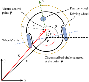
Figure 1: Sketch of the wheeled mobile robot.

To facilitate the subsequent design and analysis, we select an off-center point $\bm{P}$ as the virtual control point, which locates at a distance $\ell\neq 0$ away from $\bar{\bm{P}}$ along the longitudinal axis of the WMR [24, 25], as shown in Fig. 1. Denote by $\mathbf{x}:=[x,y]^{\top}\in\mathbb{R}^{2}$ and $\theta$ the position and heading angle of $\bm{P}$, respectively. We have the following change of coordinates:

$$\left\{\begin{aligned} &x:=\bar{x}+\ell\cos\theta,\\ &y:=\bar{y}+\ell\sin\theta,\\ &\theta:=\bar{\theta}.\end{aligned}\right.$$ (2)

In view of (1) and (2), the kinematics of $\mathbf{x}$ is given by

$$\dot{\mathbf{x}}=\mathbf{R}(\theta)(\mathbf{u}+\mathbf{u}_{d}),$$ (3)

where $\mathbf{R}(\theta)\in\mathbb{R}^{2\times 2}$ is defined as

$$\mathbf{R}(\theta):=\left[\begin{matrix}\cos\theta&-\ell\sin\theta\\ \sin\theta&\ell\cos\theta\\ \end{matrix}\right],$$ (4)

which is full rank. By setting $|\ell|\leq 1$, it follows that $\|\mathbf{R}(\theta)\|=\max\{1,|\ell|\}=1$ and $\|\mathbf{R}^{-1}(\theta)\|=\max\{1,1/|\ell|\}=1/\ell$.

Assumption 1.

The disturbance $\mathbf{u}_{d}$ is bounded by an unknown constant $d=\sup_{t\geq 0}\|\mathbf{u}_{d}(t)\|$, that is, $\|\mathbf{u}_{d}\|\leq d$.

Remark 1.

The full rank of $\mathbf{R}(\theta)$ enables us to freely control the position of the WMR (specifically, the virtual control point $\bm{P}$) without being restricted by nonholonomic constraints.

II-B Operating environment

Consider a WMR operating inside a closed compact convex workspace $\mathcal{W}^{\ast}\subset\mathbb{R}^{2}$, punctured by a set of $n\in\mathbb{N}$ obstacles $\mathcal{O}_{i}^{\ast}$, $i\in\mathbb{I}:=\{1,2,...,n\}$, which are represented by open balls with centers $\mathbf{c}_{i}\in\mathbb{R}^{2}$ and radii $r_{i}>0$. A circumscribed circle centered at $\bm{P}$ with radius $r>0$ is constructed, which is the smallest circle enclosing the WMR (see Fig. 1). To ensure that the WMR can navigate freely between any of the obstacles in $\mathcal{W}^{\ast}$, we make the following assumption:

Assumption 2.

The $n$ obstacles are separated from each other by a clearance of at least

$${\rm d}(\mathcal{O}_{i}^{\ast},\mathcal{O}_{j}^{\ast})>2(r+h),~{}\forall i,j\in\mathbb{I},~{}i\neq j,$$ (5)

and from the boundary of the workspace $\mathcal{W}^{\ast}$ as

$${\rm d}(\mathcal{O}_{i}^{\ast},\partial\mathcal{W}^{\ast})>2r+h,~{}\forall i\in\mathbb{I},$$ (6)

where $h>0$ is a constant.

For ease of design, the WMR is considered as a point (i.e., the virtual control point $\bm{P}$), by transferring the volume of the circumscribed circle to the other workspace entities. Then, for the point $\bm{P}$, the workspace is defined as

$$\mathcal{W}:=\{\mathbf{x}\in\mathbb{R}^{2}\mid\text{d}_{\complement\mathcal{W}^{\ast}}(\mathbf{x})\geq r\},$$ (7)

and the obstacle regions are defined as the following pairwise disjoint spherical subsets of $\mathbb{R}^{2}$:

$$\mathcal{O}_{i}:=\{\mathbf{x}\in\mathbb{R}^{2}\mid\beta_{i}(\mathbf{x})<0\},~{}i\in\mathbb{I},$$ (8)

where $\beta_{i}(\mathbf{x}):=\|\mathbf{x}-\mathbf{c}_{i}\|-(r+r_{i})$. Thus, the free space of $\bm{P}$ is given by the closed set $\mathcal{X}:=\mathcal{W}\setminus\mathcal{O}$ with $\mathcal{O}:=\cup_{i=1}^{n}\mathcal{O}_{i}$. To enhance the safety, a safety margin of size $0<\epsilon<h$ is introduced (see the light blue regions in Fig. 2), which results in an eroded workspace $\mathcal{W}^{\epsilon}:=\{\mathbf{x}\in\mathbb{R}^{2}\mid\text{d}_{\complement\mathcal{W}^{\ast}}(\mathbf{x})\geq r+\epsilon\}$ and $n$ augmented obstacle regions $\mathcal{O}_{i}^{\epsilon}:=\{\mathbf{x}\in\mathbb{R}^{2}\mid\beta_{i}(\mathbf{x})<\epsilon\}$, $i\in\mathbb{I}$. By doing so, the free space of $\bm{P}$ reduces to $\mathcal{X}_{\epsilon}:=\mathcal{W}^{\epsilon}\setminus\mathcal{O}^{\epsilon}$ with $\mathcal{O}^{\epsilon}:=\cup_{i=1}^{n}\mathcal{O}_{i}^{\epsilon}$.

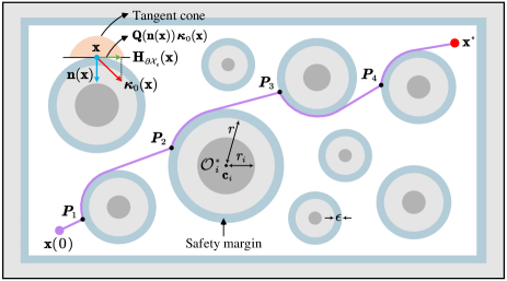
Figure 2: Schematic diagram of the operating environment. The dark gray balls denote the obstacles $\mathcal{O}_{i}^{\ast}$, $i\in\mathbb{I}$, the light gray regions denote the augmented workspace boundary and obstacles, whereas the light blue regions denote the safety margin.

II-C Problem formulation

The collision-free navigation problem for the WMR is now formulated as follows:

Problem 1.

Consider the WMR kinematics (3) under Assumptions 1 and 2. The objective is to develop a control law $\mathbf{u}$ that derives the virtual control point $\bm{P}$ from almost all initial configurations $\mathbf{x}(0)\in\mathcal{X}_{\epsilon}$ to a designated goal $\mathbf{x}^{\ast}\in\text{int}(\mathcal{X}_{\epsilon})$, without colliding with any obstacles along the route.

III Main Results

To solve Problem 1, we propose a closed-form robot navigation scheme that integrates a path planner and a tube-following controller. The block diagram of this scheme is depicted in Fig. 3. The path planner explicitly considers the safety margin and generates a collision-free reference trajectory $\mathbf{x}_{d}$ in the free space $\mathcal{X}{\epsilon}$, using tangent cones and the well-known Nagumo’s invariance theorem. In the control module, an adaptive tube-following controller is designed to track the planned trajectory in the presence of unknown disturbances, while ensuring that the position $\mathbf{x}$ of $\bm{P}$ stays within a predefined tube around the reference trajectory $\mathbf{x}_{d}$. Under this framework, if the radius of the tube is set less than the width $\epsilon$ of the safety margin, then the actual motion trajectory of $\mathbf{x}$ will remain within the set $\mathcal{X}$, thus achieving safe robot motions.

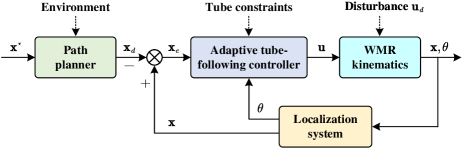
Figure 3: Block diagram of the collision-free navigation scheme.

III-A Preliminaries

The definition of tangent cones and Nagumo’s theorem that are necessary for collision-free path planning are given.

Definition 1 (Bouligand’s tangent cone [26]).

Given a closed set $\mathcal{F}\in\mathbb{R}^{n}$, the tangent cone to $\mathcal{F}$ at a point $\mathbf{x}\in\mathbb{R}^{n}$ is the subset of $\mathbb{R}^{n}$ defined by

$$\mathbf{T}_{\mathcal{F}}(\mathbf{x}):=\left\{\mathbf{z}\in\mathbb{R}^{n}\mid\mathop{\lim\inf}\limits_{\tau\to 0^{+}}\dfrac{{\rm d}_{\mathcal{F}}(\mathbf{x}+\tau\mathbf{z})}{\tau}=0\right\}.$$

The tangent cone $\mathbf{T}_{\mathcal{F}}(\mathbf{x})$ is a set that contains all the vectors pointing from $\mathbf{x}$ inside or tangent to $\mathcal{F}$, while for $\mathbf{x}\notin\mathcal{F}$, $\mathbf{T}_{\mathcal{F}}(\mathbf{x})=\emptyset$. Since for all $\mathbf{x}\in\text{int}(\mathcal{F})$, we have $\mathbf{T}_{\mathcal{F}}(\mathbf{x})=\mathbb{R}^{n}$, the tangent cone $\mathbf{T}_{\mathcal{F}}(\mathbf{x})$ is non-trivial only on the boundary $\partial\mathcal{F}$. Next, we recall the Nagumo’s invariance theorem.

Theorem 1 (Nagumo 1942 [27]).

Consider the system $\dot{\mathbf{x}}(t)=\mathbf{f}(\mathbf{x}(t))$ and assume that it admits a unique solution in forward time for each initial condition $\mathbf{x}(0)$ in an open set $\mathcal{O}$. Then, the closed set $\mathcal{F}\subset\mathcal{O}$ is forward invariant iff

$$\mathbf{f}(\mathbf{x})\in\mathbf{T}_{\mathcal{F}}(\mathbf{x}),~{}\forall\mathbf{x}\in\mathcal{F}.$$ (9)

An intuitive interpretation of Nagumo’s theorem is that if the vector field $\mathbf{f}(\mathbf{x})$ points inside or is tangent to the set $\mathcal{F}$ at each point $\mathbf{x}\in\mathcal{F}$, then $\mathcal{F}$ is forward invariant. As stated earlier, $\mathbf{T}_{\mathcal{F}}(\mathbf{x})$ is non-trivial only on $\partial\mathcal{F}$, thus it is only necessary to check (9) for the boundary points.

Lemma 1.

Given any constant $b>0$, the following inequalities hold for all $0\leq q<b$:

$$\frac{q}{b}\leq\ln\dfrac{b}{b-q}\leq\dfrac{q}{b-q}.$$

Proof. Define two functions $h_{1}(q):=q/(b-q)-\ln(b/(b-q))$ and $h_{2}(q):=\ln(b/(b-q))-q/b$. After simple calculations, it follows that

$$\dfrac{\partial h_{1}(q)}{\partial q}=\dfrac{q}{(b-q)^{2}}\geq 0,~{}\dfrac{\partial h_{2}(q)}{\partial q}=\dfrac{q}{b(b-q)}\geq 0,$$

for all $0\leq q<b$. Hence, $h_{i}(q)$, $i=1,2$ are nondecreasing functions of $q$, and $h_{i}(q)\geq h_{i}(0)=0$ for all $0\leq q<b$. The latter implies that Lemma 1 holds. $\hfill\Box$

III-B Path planing based on tangent cones

Based on Bouligand’s tangent cones and Nagumo’s theorem, a safe path planning approach is proposed, which can guide the virtual control point $\bm{P}$ towards the goal $\mathbf{x}^{\ast}$ (motion-to-goal) from almost all initial conditions $\mathbf{x}(0)\in\mathcal{X}_{\epsilon}$, while ensuring forward invariance of the free space $\mathcal{X}_{\epsilon}$ (collision avoidance). We neglect the disturbance $\mathbf{u}_{d}$ in (3) and consider a control law of the following form

$$\mathbf{u}=\mathbf{R}^{-1}(\theta)\bm{\tau},$$ (10)

where $\bm{\tau}\in\mathbb{R}^{2}$ is a virtual control law to be designed. Then, substituting (10) into (3), one gets

$$\dot{\mathbf{x}}=\bm{\tau}.$$ (11)

According to Nagumo’s theorem, it is sufficient to address the collision-free path planning problem by solving the following constrained optimization problem

$$\begin{split}\min\limits_{\bm{\tau}}&~{}\|\bm{\tau}-\bm{\kappa}_{0}(\mathbf{x})\|,\\ \text{s.t.}&~{}\bm{\tau}\in\mathbf{T}_{\mathcal{{X}}_{\epsilon}}(\mathbf{x}),~{}\forall\mathbf{x}\in\mathcal{X}_{\epsilon},\end{split}$$ (12)

where $\bm{\kappa}_{0}(\mathbf{x})$ is a nominal control law for motion-to-goal and is designed here as the following smooth function:

$$\bm{\kappa}_{0}(\mathbf{x})=-k_{0}(\mathbf{x})(\mathbf{x}-\mathbf{x}^{\ast}),$$ (13)

with $k_{0}(\mathbf{x})>0$ given by

$$k_{0}(\mathbf{x}):=\dfrac{\alpha}{\sqrt{\|\mathbf{x}-\mathbf{x}^{\ast}\|^{2}+\beta^{2}}},$$ (14)

where $\alpha$ and $\beta$ are positive design constants. From (13) and (14), it follows that $\|\bm{\kappa}_{0}(\mathbf{x})\|\leq\alpha$, which allows us to generate a saturated nominal vector field. The problem (12) is clearly a nearest point problem, which has an explicit solution that will be demonstrated in the following.

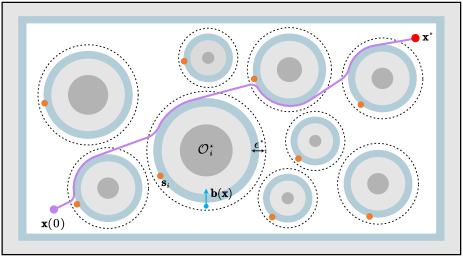
Figure 4: The resulting smooth navigation trajectories maintains a safety margin of size $\epsilon$ (light blue regions) from the workspace boundary and obstacles. The dashed circles denote the influence regions from each obstacle. Moreover, the orange points are the unstable stationary points associated with each obstacles.

The robot workspace $\mathcal{W}^{\ast}$ is a convex set, so does $\mathcal{W}^{\epsilon}$, which together with the fact that $\mathbf{x}^{\ast}\in\text{int}(\mathcal{X}_{\epsilon})$ suggests that for all $\mathbf{x}\in\partial\mathcal{W}^{\epsilon}$, $\bm{\kappa}_{0}(\mathbf{x})$ points inside the free space $\mathcal{X}_{\epsilon}$ (i.e., $\bm{\kappa}_{0}(\mathbf{x})\in\mathbf{T}_{\mathcal{{X}}_{\epsilon}}(\mathbf{x})$) and thus is a solution to (12). Moreover, for all $\mathbf{x}\in\text{int}(\mathcal{X}_{\epsilon})$, it follows that $\bm{\kappa}_{0}(\mathbf{x})$ is also the solution to (12). Next we check the obstacle boundary points $\mathbf{x}\in\partial\mathcal{O}^{\epsilon}$. As $\partial\mathcal{O}^{\epsilon}$ is a smooth hypersurface of $\mathbb{R}^{2}$, which is orientable, there exists a continuously differentiable map (known as the Gauss map [28]) $\mathbf{n}:\partial\mathcal{O}^{\epsilon}\to\mathbb{S}^{1}$ such that for all $\mathbf{x}\in\partial\mathcal{O}^{\epsilon}$, $\mathbf{n}(\mathbf{x})$ is the outward unit normal vector to $\partial\mathcal{O}^{\epsilon}$. As clearly seen in Fig. 2, the tangent cone at any $\mathbf{x}\in\partial\mathcal{O}^{\epsilon}$ is a half-space

$$\mathbf{T}_{\mathcal{X}_{\epsilon}}(\mathbf{x}):=\{\mathbf{y}\in\mathbb{R}^{2}\mid(\mathbf{y}-\mathbf{x})^{\top}\mathbf{n}(\mathbf{x})\leq 0\},$$ (15)

which is a convex function. Thus, (12) has a unique solution. Based on the above argument, it is known that if $\mathbf{x}\in\mathcal{X}_{\epsilon}\setminus\partial\mathcal{O}^{\epsilon}$ or $\mathbf{x}\in\partial\mathcal{O}^{\epsilon}$ and $\bm{\kappa}_{0}^{\top}(\mathbf{x})\mathbf{n}(\mathbf{x})\leq 0$, then $\bm{\kappa}_{0}(\mathbf{x})$ is a solution to (12). On the other hand, if $\mathbf{x}\in\mathcal{O}^{\epsilon}$ and $\bm{\kappa}_{0}^{\top}(\mathbf{x})\mathbf{n}(\mathbf{x})>0$, the closest point of (12) is obtained by the orthogonal projection $\mathbf{Q}(\mathbf{n}(\mathbf{x})):=\mathbf{I}_{2}-\mathbf{n}(\mathbf{x})\mathbf{n}^{\top}(\mathbf{x})$ onto the tangent hyperplane of $\partial\mathcal{X}_{\epsilon}$, defined by $\mathbf{H}_{\partial\mathcal{X}_{\epsilon}}(\mathbf{x}):=\{\mathbf{y}\in\mathbb{R}^{2}\mid(\mathbf{y}-\mathbf{x})^{\top}\mathbf{n}(\mathbf{x})=0\}$. Then, a general solution to (12) is as follows:

$$\bm{\tau}(\mathbf{x})=\left\{\begin{split}&\bm{\kappa}_{0}(\mathbf{x}),&\text{if}~{}&\text{d}_{\mathcal{O}}(\mathbf{x})>\epsilon~{}\text{or}\\ &&&\bm{\kappa}_{0}^{\top}(\mathbf{x})\mathbf{n}(\mathbf{x})\leq 0,\\ &\mathbf{Q}(\mathbf{n}(\mathbf{x}))\bm{\kappa}_{0}(\mathbf{x}),&\text{if}~{}&\text{d}_{\mathcal{O}}(\mathbf{x})=\epsilon~{}\text{and}\\ &&&\bm{\kappa}_{0}^{\top}(\mathbf{x})\mathbf{n}(\mathbf{x})>0.\end{split}\right.$$ (16)

By inspecting (16), we find that the resulting vector field is discontinuous at some boundary points $\mathbf{x}\in\partial\mathcal{O}^{\epsilon}$ like $\bm{P}_{1}-\bm{P}_{4}$ in Fig. 2. To address this issue, a continuous version of (16) is proposed in the sequel. Following the line of [4], we specify an influence region for each obstacle (marked by the dashed line in Fig. 4), which is defined as $\{\mathbf{x}\in\mathbb{R}^{2}\mid\text{d}_{\mathcal{O}_{i}}(\mathbf{x})\leq\epsilon^{\ast}\}$, where $\epsilon^{\ast}\in(\epsilon,h]$ and $i\in\mathbb{I}$. Obstacle avoidance is activated only when the position $\mathbf{x}$ of $\bm{P}$ enters the influence regions of obstacles. To proceed, a bearing vector is defined as

$$\mathbf{b}(\mathbf{x}):=\dfrac{\mathbf{P}_{\partial\mathcal{O}}(\mathbf{x})-\mathbf{x}}{\|\mathbf{P}_{\partial\mathcal{O}}(\mathbf{x})-\mathbf{x}\|}=\dfrac{\mathbf{P}_{\partial\mathcal{O}}(\mathbf{x})-\mathbf{x}}{\text{d}_{\mathcal{O}}(\mathbf{x})}.$$ (17)

for all $\mathbf{x}$ with $\epsilon\leq\text{d}_{\mathcal{O}}(\mathbf{x})\leq\epsilon^{\ast}$. Since $\text{d}(\mathcal{O}_{i}^{\ast},\mathcal{O}_{j}^{\ast})>2(r+h)$, $\forall i,j\in\mathbb{I}$, $i\neq j$ (referring to (5) in Assumption 2) and $\epsilon^{\ast}\leq h$, there can be only one obstacle $\mathcal{O}_{i}$, $i\in\mathbb{I}$ such that $\text{d}_{\mathcal{O}}(\mathbf{x})=\text{d}_{\mathcal{O}_{i}}(\mathbf{x})\leq\epsilon^{\ast}$. With this in mind, $\mathbf{b}(\mathbf{x})$ in (17) can be computed by $\mathbf{b}(\mathbf{x})=(\mathbf{c}_{i}-\mathbf{x})/\|\mathbf{c}_{i}-\mathbf{x}\|$. Note that when $\mathbf{x}\in\partial\mathcal{O}_{\epsilon}$, $\mathbf{b}(\mathbf{x})$ is equivalent to the Gauss map $\mathbf{n}(\mathbf{x})$.

Now the control law (16) is modified as

$$\bm{\tau}(\mathbf{x})=\left\{\begin{split}&\bm{\kappa}_{0}(\mathbf{x}),&\text{if}~{}&\text{d}_{\mathcal{O}}(\mathbf{x})>\epsilon^{\ast}~{}\text{or}\\ &&&\bm{\kappa}_{0}^{\top}(\mathbf{x})\mathbf{b}(\mathbf{x})\leq 0,\\ &\mathbf{\Pi}(\mathbf{x})\bm{\kappa}_{0}(\mathbf{x}),&\text{if}~{}&\text{d}_{\mathcal{O}}(\mathbf{x})\leq\epsilon^{\ast}~{}\text{and}\\ &&&\bm{\kappa}_{0}^{\top}(\mathbf{x})\mathbf{b}(\mathbf{x})>0,\end{split}\right.$$ (18)

with

$$\mathbf{\Pi}(\mathbf{x}):=\mathbf{I}_{2}-\phi(\text{d}_{\mathcal{O}}(\mathbf{x}))\mathbf{b}(\mathbf{x})\mathbf{b}^{\top}(\mathbf{x}),$$ (19)

where $\phi(\text{d}_{\mathcal{O}}(\mathbf{x}))\in\mathbb{R}$ is a $C^{1}$ bump function that smoothly transitions from $1$ to $0$ on the interval $\text{d}_{\mathcal{O}}(\mathbf{x})\in[\epsilon,\epsilon^{\ast}]$, that is to say, its first derivatives equal to zero at the endpoints of the interval $[\epsilon,\epsilon^{\ast}]$. A simple choice of $\phi(\text{d}_{\mathcal{O}}(\mathbf{x}))$ is

$$\phi(\text{d}_{\mathcal{O}}(\mathbf{x}))=\left\{\begin{split}&1,&\text{if}~{}&\text{d}_{\mathcal{O}}(\mathbf{x})\leq\epsilon,\\ &\lambda(\text{d}_{\mathcal{O}}(\mathbf{x})),&\text{if}~{}&\epsilon<\text{d}_{\mathcal{O}}(\mathbf{x})<\epsilon^{\ast},\\ &0,&\text{if}~{}&\text{d}_{\mathcal{O}}(\mathbf{x})\geq\epsilon^{\ast},\end{split}\right.$$ (20)

with

$$\lambda(\text{d}_{\mathcal{O}}(\mathbf{x}))=\dfrac{1}{2}\left[1-\cos\left(\pi\dfrac{\epsilon^{\ast}-\text{d}_{\mathcal{O}}(\mathbf{x})}{\epsilon^{\ast}-\epsilon}\right)\right].$$ (21)

One can verify that $\phi(\epsilon)=1$, $\phi(\epsilon^{\ast})=0$, and

$$\left.\dfrac{d\phi(\text{d}_{\mathcal{O}}(\mathbf{x}))}{d\text{d}_{\mathcal{O}}(\mathbf{x})}\right|_{\text{d}_{\mathcal{O}}(\mathbf{x})=0~{}\text{or}~{}\epsilon^{\ast}}=0.$$

Since the nominal control law, $\bm{\kappa}_{0}(\mathbf{x})$, the bearing vector, $\mathbf{b}(\mathbf{x})$, and the bump function, $\phi(\text{d}_{\mathcal{O}}(\mathbf{x}))$, are continuously differentiable, the resulting control law $\bm{\tau}(\mathbf{x})$ in (18) is continuous and piecewise continuously differentiable on the domain $\mathcal{X}$. It is not differentiable only at those points satisfying $\text{d}_{\mathcal{O}}(\mathbf{x})\leq\epsilon^{\ast}$ and $\bm{\kappa}_{0}^{\top}(\mathbf{x})\mathbf{b}(\mathbf{x})=0$. Now the main result of the path planning problem is summarized in the following theorem.

Theorem 2.

Consider the single-integrator kinematics defined by (11). Given that $\mathbf{x}^{\ast}\in\text{int}(\mathcal{X}_{\epsilon})$ and the obstacles $\mathcal{O}_{i}^{\ast}$, $i\in\mathbb{I}$ satisfying Assumption 2, the continuous control law (18) with $\bm{\kappa}_{0}(\mathbf{x})$ given by (13) can guarantee that:

1. The free space $\mathcal{X}_{\epsilon}$ in (7) is forward invariant.

2. For any $\mathbf{x}(0)\in\mathcal{X}_{\epsilon}$, the kinematics (11) admits a unique solution in forward time, which asymptotically converges to the set $\{\mathbf{x}^{\ast}\}\cup_{i=1}^{n}\mathcal{S}_{i}$ with $\mathcal{S}_{i}$ given by

   $$\mathcal{S}_{i}:=\left\{\mathbf{x}\in\mathcal{X}_{\epsilon}\bigg{|}{\rm d}_{\mathcal{O}_{i}}(\mathbf{x})=\epsilon,~{}\dfrac{\bm{\kappa}_{0}^{\top}(\mathbf{x})\mathbf{b}(\mathbf{x})}{\|\bm{\kappa}_{0}(\mathbf{x})\|}=1\right\}.$$ (22)

3. The undesired stationary points $\mathbf{s}_{i}\in\mathcal{S}_{i}$, associated with obstacles $\mathcal{O}_{i}$, are locally unstable and only have a stable manifold of measure zero.

4. The equilibrium point $\mathbf{x}=\mathbf{x}^{\ast}$ is almost globally asymptotically stable and locally exponentially stable.

Proof. The proof is relegated to Appendix. $\hfill\Box$

Remark 2.

The proposed safe path planning scheme offers an analytical solution and thus is computationally much more efficient than the optimization-based methods. Moreover, unlike the navigation functions, the scheme can achieve almost global asymptotic convergence without requiring unknown parameter tuning, making it easy to implement in practice.

Remark 3.

A smooth and saturated nominal control law (18) is proposed, instead of the traditional proportional control law $k_{0}(\mathbf{x})=-k(\mathbf{x}-\mathbf{x}^{\ast})$ [4, 21], with the aim of generating a saturated vector field (18). This is justified by the inequality $\|\bm{\tau}(\mathbf{x})\|\leq\|\bm{\kappa}_{0}(\mathbf{x})\|\leq\alpha$, where the equality $\|\bm{\Pi}(\mathbf{x})\|=1$ has been used. In fact, different types of saturation functions can be used to design $\kappa_{0}(\mathbf{x})$ as an alternative, such as the standard saturation function $\text{sat}(\cdot)$, hyperbolic tangent function $\tanh(\cdot)$, arctangent function $\text{arctan}(\cdot)$, etc. However, it is worth noting that these functions may result in the nominal control direction not aligning directly with the desired position, which in turn leads to an unnecessarily long path.

III-C Adaptive tube-following control

The planning algorithm introduced in Sec. III-B can generate a collision-free reference trajectory for the WMR. To avoid conflicts of notations, the reference trajectory is denoted as $\mathbf{x}_{d}$, which is governed by

$$\dot{\mathbf{x}}_{d}=\bm{\tau}_{d},$$ (23)

where $\bm{\tau}_{d}$ is given by (18) but with $\mathbf{x}$ replaced by $\mathbf{x}_{d}$. Let us define the position tracking error as $\mathbf{x}_{e}:=\mathbf{x}-\mathbf{x}_{d}$ and impose an inequality constraint on it as follows:

$$\|\mathbf{x}_{e}(t)\|^{2}<\rho^{2},$$ (24)

where $\rho>0$ is a user-defined constant. At each time instance, the actual position $\mathbf{x}$ of the virtual control point $\bm{P}$ is allowed to stay within a 1-sphere of radius $\rho$ and center $\mathbf{x}_{d}(t)$. Unifying all such spheres along $t$ forms a tube around $\mathbf{x}_{d}(t)$, as shown in Fig. 5. Since a safety margin is considered in the planning module, if the tube radius is taken no larger than the size $\epsilon$ of the safety margin and (24) holds for all $t\geq 0$, then the actual trajectory $\mathbf{x}(t)$ will remain within the predefined tube without colliding with any actual obstacles, that is, $\mathbf{x}\in\mathcal{X}$.

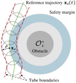
Figure 5: Illustration of the predefined tube.

In the following, an adaptive tube-following controller is developed to achieve high-precision trajectory tracking, while ensuring that $\mathbf{x}(t)$ evolves within the tube defined by (24). To this end, we define a transformed error

$$\xi(t):=\dfrac{\|\mathbf{x}_{e}(t)\|^{2}}{\rho^{2}}.$$ (25)

Taking the time derivative of (25), whilst using (3) and (23), one can easily get

$$\dot{\xi}=\dfrac{2}{\rho^{2}}\mathbf{x}_{e}^{\top}[\mathbf{R}(\theta)(\mathbf{u}+\mathbf{u}_{d})-\bm{\tau}_{d}].$$ (26)

Inspecting (25) reveals that $0\leq\xi(t)<1$ is equivalent to (24), and $\xi(t)=0$ only when $\mathbf{x}_{e}(t)=\mathbf{0}$. Therefore, the tube-following control problem boils down to achieving $\lim_{t\to\infty}\xi(t)=0$, while ensuring $0\leq\xi(t)<1$, $\forall t\geq 0$, via a properly-designed controller. To achieve this, the following logarithmic barrier function is considered

$$L=\dfrac{1}{2}\ln\dfrac{1}{1-\xi}.$$ (27)

Let $\mathbf{z}:=\mathbf{x}_{e}/(\rho^{2}(1-\xi))$. Then, evaluating the time derivative of $L$ along (26) yields

$$\dot{L}= ~{}\mathbf{z}^{\top}[\mathbf{R}(\theta)(\mathbf{u}+\mathbf{u}_{d})-\bm{\tau}_{d}]$$

$$\leq ~{}\mathbf{z}^{\top}(\mathbf{R}(\theta)\mathbf{u}-\bm{\tau}_{d})+d\|\mathbf{z}\|,$$ (28)

wherein we have used the fact that $\|\mathbf{R}(\theta)\|=1$.

The adaptive control law is designed as

$$\mathbf{u}=\mathbf{R}^{-1}(\theta)(-k\mathbf{x}_{e}+\bm{\tau}_{d}-\bm{\varpi}),$$ (29)

with

$$\bm{\varpi}:=\dfrac{\hat{d}^{2}\mathbf{z}}{\sqrt{\hat{d}^{2}\|\mathbf{z}\|^{2}+\varphi^{2}}},$$ (30)

where $\hat{d}$ denotes the estimate of $d$ (see Assumption 1 for its definition) and is updated by a projection-based adaptive law. Suppose $d\in\Omega:=\{\nu\in\mathbb{R}\mid 0\leq\nu\leq d_{m}\}$ and let $\Omega_{\delta}:=\{\nu\in\mathbb{R}\mid 0\leq\nu\leq d_{m}+\delta\}$, where $d_{m}>0$ and $\delta>0$ are known constants. Inspired by [29], the adaptive law is derived as

$$\dot{\hat{d}}=\text{Proj}(\hat{d},\Phi),~{}\Phi:=\|\mathbf{z}\|-\gamma\hat{d},$$ (31)

with

$$\text{Proj}(\hat{d},\Phi)=\left\{\begin{split}&\eta\Phi,&{\rm if}~{}&1)~{}0\leq\hat{d}<d_{m}~{}\text{or}\\ &&~{}&2)~{}\hat{d}\geq d_{m}~{}\text{and}~{}\Phi\leq 0,\\ &\eta\breve{\Phi},&{\rm if}~{}&3)~{}\hat{d}\geq d_{m}~{}\text{and}~{}\Phi>0,\end{split}\right.$$ (32)

where $\eta,\,\gamma>0$ are design constants and

$$\breve{\Phi}=\left(1-\dfrac{\hat{d}-d_{m}}{\delta}\right)\Phi.$$ (33)

Note that the projection operator $\text{Proj}(\hat{d},\Phi)$ is locally Lipschitz in $(\hat{d},\Phi)$ [29]. Choosing the initial condition of (31) as $\hat{d}(0)\in\Omega_{\delta}$, we will now demonstrate that

$$\hat{d}(0)\in\Omega_{\delta}\Rightarrow\hat{d}(t)\in\Omega_{\delta},~{}\forall t\geq 0.$$ (34)

In Cases 1 and 2, the adaptive law (31) reduces to

$$\dot{\hat{d}}=\eta(\|\mathbf{z}\|-\gamma\hat{d}).$$ (35)

Solving (35) yields

$$\hat{d}(t)=e^{-\eta\gamma t}\hat{d}(t_{0})+\eta\int_{t_{0}}^{t}\|\mathbf{z}(\tau)\|e^{-\eta\gamma(t-t_{0}-\tau)}d\tau,$$ (36)

where $t_{0}\geq 0$ marks the beginning of each time interval during which Cases 1 and 2 hold. Moreover, in these two cases, (34) holds as a result of the given conditions. In Case 3, however, (31) becomes

$$\dot{\hat{d}}=\dfrac{\delta+d_{m}-\hat{d}}{\delta}\Phi,$$ (37)

which implies that $\hat{d}$ decreases when $\hat{d}>\delta+d_{m}$ and increases if $\hat{d}<\delta+d_{m}$ until it reaches $\delta+d_{m}$ such that $\dot{\hat{d}}=0$. Therefore, the adaptive law (31) ensures that (34) holds. Let us define the parameter estimation error as $\tilde{d}:=\hat{d}-d$.

Theorem 3.

Consider the WMR kinematics (3) under Assumption 1 and suppose that $d\in\Omega$. Given the initial position $\mathbf{x}(0)$ satisfying (25), then the adaptive controller (29), together with the projection-based update law (31), can steer $\mathbf{x}$ to track the reference trajectory $\mathbf{x}_{d}$ given by (23) along with the predefined tube (25), while ensuring uniform ultimate boundedness of the position error $\mathbf{x}_{e}$ and the estimation error $\tilde{d}$.

Proof. Consider the Lyapunov function candidate (LFC):

$$V=L+\dfrac{1}{2\eta}\tilde{d}^{2}.$$ (38)

Taking the derivative of $V$ and using (III-C) and (29) lead to

$$\dot{V}\leq-k\mathbf{z}^{\top}\mathbf{x}_{e}-\mathbf{z}^{\top}\bm{\varpi}+\hat{d}\|\mathbf{z}\|+\dfrac{1}{\eta}\tilde{d}(\dot{\hat{d}}-\eta\|\mathbf{z}\|).$$ (39)

Invoking the inequality $|\nu|\leq\nu^{2}/\sqrt{\nu^{2}+\varphi^{2}}+\varphi$ for any $\nu\in\mathbb{R}$ and $\varphi>0$, one gets $-\mathbf{z}^{\top}\bm{\varpi}+\hat{d}\|\mathbf{z}\|\leq\varphi$. In addition, noting (26), (III-C), and Lemma 1, it follows that $-k\mathbf{z}^{\top}\mathbf{x}_{e}=-k\xi/(1-\xi)\leq-2kL$ for all $0\leq\xi<1$. As a result, (39) reduces to

$$\dot{V}\leq-2kL+\varphi+\dfrac{1}{\eta}\tilde{d}(\dot{\hat{d}}-\eta\|\mathbf{z}\|),$$ (40)

on the set $0\leq\xi<1$. To proceed, we consider three cases in (32). For Cases 1 and 2, it follows from (35) that

$$\tilde{d}(\dot{\hat{d}}-\eta\|\mathbf{z}\|)=-\eta\gamma\tilde{d}\hat{d}.$$ (41)

While for Case 3, we have

$$\tilde{d}(\dot{\hat{d}}-\eta\|\mathbf{z}\|)=-\eta\gamma\tilde{d}\hat{d}-\dfrac{\eta\tilde{d}(\hat{d}-d_{m})\Phi}{\delta}\leq-\eta\gamma\tilde{d}\hat{d},$$ (42)

which is true because $\tilde{d}\geq 0$, $\hat{d}-d_{m}\geq 0$, and $\Phi>0$ according to the conditions specified in Case 3. In view of (41) and (42), one can easily get

$$\dot{V} \leq-2kL-\gamma\tilde{d}\hat{d}+\varphi$$

$$\leq-2kL-\dfrac{\gamma}{2}\tilde{d}^{2}+c$$

$$\leq-aV+c,$$ (43)

where $a:=\min\{2k,\eta\gamma\}>0$ and $c:=\gamma d^{2}/2+\varphi>0$.

Integrating both sides of (III-C) over $[0,\infty)$ yields

$$V(t)\leq\left(V(0)-\dfrac{c}{a}\right)e^{-at}+\dfrac{c}{a},~{}\forall t\geq 0,$$ (44)

showing that $V\in\mathcal{L}_{\infty}$ and hence $L\in\mathcal{L}_{\infty}$. The later implies that $0\leq\xi(t)<1$ for all $t\geq 0$. As a consequence, $\mathbf{x}$ keeps within the predefined tube (25). As $L(t)\leq V(t)$, it follows from (25) and (27) that $\|\mathbf{x}_{e}(t)\|\leq\rho\sqrt{1-e^{-2V(t)}}$. In addition, $\tilde{d}^{2}/(2\eta)\leq V(t)$ leads to $|\tilde{d}(t)|\leq\sqrt{2\eta V(t)}$. As shown in (44), $V(t)$ is eventually bounded by $c/a$, whereby one can get

$$\mathop{\lim\sup}\limits_{t\to\infty}\|\mathbf{x}_{e}(t)\|\leq\rho\sqrt{1-e^{-2c/a}},~{}\mathop{\lim\sup}\limits_{t\to\infty}|\tilde{d}(t)|\leq\sqrt{2\eta c/a}.$$

Thus, $\mathbf{x}_{e}$ and $\tilde{d}$ are uniformly ultimately bounded. $\hfill\Box$

Remark 4.

Based on the facts that $\|\mathbf{R}^{-1}(\theta)\|=1/\ell$ ($\ell<1$), $\|\bm{\tau}_{d}\|\leq\|\bm{\kappa}_{0}(\mathbf{x}_{d})\|\leq\alpha$ (noting (13), (14), and $\|\bm{\Pi}(\mathbf{x}_{d})\|=1$), and $\|\bm{\varpi}\|\leq\hat{d}\leq d_{m}+\sigma$ (noting (34)), it can be easily verified that the adaptive controller (29) is bounded and its bound can be explicitly expressed as

$$\|\mathbf{u}\|\leq\dfrac{1}{\ell}(k\rho+\alpha+d_{m}+\delta).$$ (45)

This implies that the input constraint $\|\mathbf{u}\|\leq u_{m}$ can be met by judiciously choosing the design parameters such that $k\rho+\alpha+d_{m}+\delta\leq\ell u_{m}$. However, it is noted that achieving smaller convergence bounds for $\mathbf{x}_{e}$ and $\tilde{d}$ requires a larger value of $k$. Thus, a compromise should be reached according to the robot actuation capability and performance requirement.

Remark 5.

As defined in (1), the kinematics of $\theta$ is

$$\dot{\theta}=\omega+u_{d2},$$ (46)

where $u_{d2}$ is the second element of $\mathbf{u}_{d}$. Due to the presence of disturbances, we can only show that the right-hand side of $\eqref{eq66}$ is bounded. However, it cannot strictly converge to zero, which would lead to the continuous changes of $\theta$, even if the WMR has already reached the designated position. To address this issue, a simple approach is to halt the WMR motion once $\mathbf{x}$ enters a predefined, sufficiently small neighborhood around the goal position $\mathbf{x}^{\ast}$.

IV Simulation Results

In this section, we demonstrate the proposed control method in a $6.4\,\text{m}\times 3.4\,\text{m}$ rectangular workspace $\mathcal{W}^{\ast}$ cluttered with 8 circular obstacles, denoted as $\mathcal{O}_{i}^{\ast}$, whose centers and radii are listed in Table I. The distance between the virtual and actual control points is $\ell=0.05\,\rm m$, the radius of the circumscribed circle around $\bm{P}$ is $r=0.2\,\rm m$, and the clearance constant in Assumption 2 is $h=0.2\,\rm m$. The size of the safety margin is set to $\epsilon=0.1\,\rm m$, and the obstacle influence region is specified by $\epsilon^{\ast}=0.2\,\rm m$. The goal location is taken as $\mathbf{x}^{\ast}=[2.5,1]^{\top}\,\rm m$. Assume that the control input constraint is $u_{m}=1.5$, and the disturbance $\mathbf{u}_{d}$ is of the following form

$$\mathbf{u}_{d}=0.01\times\left[\begin{matrix}\sin(0.2t)+1\\ \cos(0.3t)-2\end{matrix}\right].$$ (47)

According to Remark 4, the planner parameters are chosen as $\alpha=0.03$ and $\beta=0.005$, while the controller parameters are chosen as $\rho=0.06$, $k=0.1$, $\psi=0.005$, $\eta=0.1$, $\gamma=0.01$, $d_{m}=0.03$, $\delta=0.005$, and $\hat{d}(0)=0.01$. The simulation duration is $500\,\rm s$, and the sample step is $0.01\,\rm s$.

We begin by verifying the efficiency of the proposed tangent cone-based path planning method (denoted as “TC-based planner”) in the absence of disturbances. For comparison purposes, the PF-based path planning method presented in [30] (denoted as “PF-based planner”) is also simulated. A slight modification is made for [30] to facilitate its implementation. The attractive and repulsive potentials are chosen as

$$U_{att}(\mathbf{x}_{d})= \dfrac{1}{2}k_{a}\|\mathbf{x}_{d}-\mathbf{x}^{\ast}\|^{2},$$

$$U_{rep}(\mathbf{x}_{d})= \dfrac{1}{2}k_{r}\left(\sum_{i=0}^{8}\dfrac{1}{\rho_{i}}\right)\|\mathbf{x}_{d}-\mathbf{x}^{\ast}\|^{2},$$

where $k_{a}$ and $k_{r}$ are positive weights, $\rho_{0}:=1-(x_{d}/2.9)^{20}-(y_{d}/1.4)^{20}$, while $\rho_{i}:=\|\mathbf{x}_{d}-\mathbf{c}_{i}\|^{2}-(r+r_{i}+\epsilon)^{2}$, $i\in\mathbb{I}$. The total velocity is then given by

$$\bm{\tau}_{d}=-\nabla U_{att}(\mathbf{x}_{d})-\nabla U_{rep}(\mathbf{x}_{d}).$$ (48)

For fair comparison, we chose the parameters of the PF-based path planner to be $k_{a}=0.05$ and $k_{r}=0.0001$, such that the two planners have nearly identical convergence times. Figure 6 shows the obtained robot navigation trajectories of both path planners starting at a set of initial positions (purple points). As can be seen, both planners can successfully guide the virtual control point $\bm{P}$ from different initial positions to the goal (red point), while avoiding all obstacle regions $\mathcal{O}_{i}^{\epsilon}$, $i=1,2,...,8$. However, the proposed planner yields shorter trajectories than the PF-based one. The comparison results of the velocity norm $\|\bm{\tau}_{d}\|$ are depicted in Fig. 7, from which it is clear that the PF-based planner requires larger velocity than the proposed one. Actually, $\bm{\tau}_{d}$ under the proposed planner is upper bounded by $\alpha=0.03$, which is consistent with our analysis in Remark 3. The above results demonstrate the effectiveness and superiority of the proposed path planner.

TABLE I: Geometrical details of the obstacles.

Index	Configuration		Index	Configuration
	Center (m)	Radius (m)		Center (m)	Radius (m)
$\mathcal{O}_{1}^{\ast}$	$[-2,-0.55]^{\top}$	$0.10$	$\mathcal{O}_{5}^{\ast}$	$[0.4,0.55]^{\top}$	$0.25$
$\mathcal{O}_{2}^{\ast}$	$[-0.9,0.85]^{\top}$	$0.10$	$\mathcal{O}_{6}^{\ast}$	$[0.7,-0.6]^{\top}$	$0.10$
$\mathcal{O}_{3}^{\ast}$	$[-0.7,-0.5]^{\top}$	$0.35$	$\mathcal{O}_{7}^{\ast}$	$[2,-0.6]^{\top}$	$0.25$
$\mathcal{O}_{4}^{\ast}$	$[-2.1,0.6]^{\top}$	$0.15$	$\mathcal{O}_{8}^{\ast}$	$[1.8,0.7]^{\top}$	$0.15$

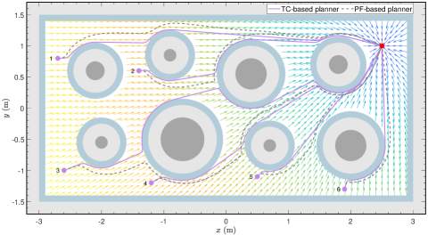
Figure 6: Navigation trajectories of the two path planners.

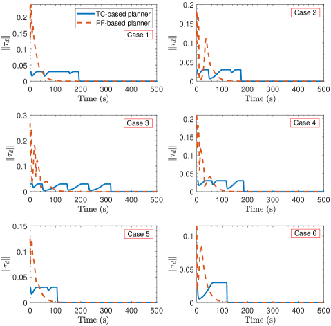
Figure 7: Velocity norms of the two path planners.

We next illustrate the performance of the proposed adaptive tube-following controller (29) (denoted as “TF controller”) in the presence of disturbance given by (47). As a case study, the trajectory starting from the 3nd initial position is selected as the reference trajectory (see Fig. 6). For comparison purposes, the extensively used proportional-integral (PI) controller of the following form is simulated:

$$\mathbf{u}=-k_{p}\mathbf{x}_{e}-k_{i}\int_{0}^{t}\mathbf{x}_{e}(\tau)\text{d}\tau,$$

where $k_{p}=0.5$ and $k_{i}=0.3$ are constant gains. Furthermore, in order to verify the robustness of the PF-based planner (48) (denoted here as “PF controller”), we execute it in the presence of disturbances and define the difference between the ideal and actual trajectories as the position tracking error $\mathbf{x}_{e}$. The closed-loop responses of these three controllers are shown in Fig. 8. In the top left subfigure of Fig. 8, the tracking error $\mathbf{x}_{e}$ under both the TF and PI controllers is shown to remain within a small neighborhood of the origin (but quantitatively, the TF controller has higher tracking accuracy than the PI controller), while satisfying the tube constraint (24). However, the PF controller yields a larger tracking error and violates the tube constraint. The latter may result in collision with obstacles or the workspace boundary. The WMR’s heading angle is plotted in the top right subfigure of Fig. 8, from which it is clear that $\theta$ under the TF and PI controllers is bounded and converges to a nearly constant value (precisely, the TF controller has a higher stability), while under the PF controller $\theta$ continuously increases. This implies that the PF controller (i.e., path planner (48)) is susceptible to disturbances. The control input norm $\|\mathbf{u}\|$ is shown in the bottom left subfigure of Fig. 8. Obviously, the control input $\mathbf{u}$ of the TF and PI controllers satisfies the magnitude limits $\|\mathbf{u}\|\leq u_{m}$, while the PF controller fails. The parameter estimate $\hat{d}$ is given in the bottom right subfigure of Fig. 8. As can be seen, $\hat{d}$ remains within the set $\Omega_{\delta}$, indicating the effectiveness of the projection adaptive law (31). Finally, the position tracking trajectory of the proposed TF controller (29) is shown in Fig. 9. Intuitively, the virtual control point $\bm{P}$ accurately tracks the reference trajectory, while remaining with the predefined tube. Therefore, the WMR reaches the goal position without colliding with any obstacles (dark gray balls), as clearly seen in Fig. 9.

Overall, the proposed integrated path planning and tube-following control scheme can successfully drive the WMR to reach the predefined goal without colliding with any obstacles, despite the presence of input disturbances.

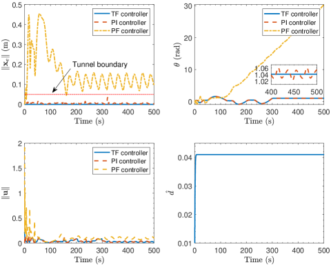
Figure 8: Closed-loop control responses.

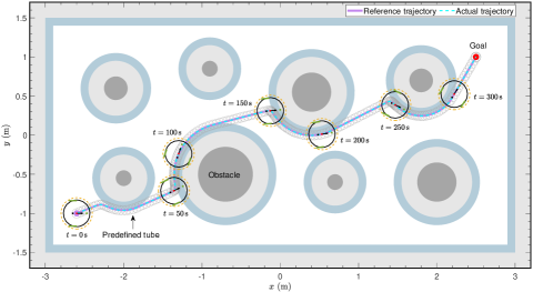
Figure 9: Position tracking trajectory with WMR snapshots.

V Experiments

In this section, several experiments are carried out to verify the effectiveness of the proposed method.

V-A Experimental setup

In the experiments, several simple scenarios are considered where the WMR is tasked with navigating towards a designated goal location, while ensuring avoidance of any obstacles en route. The experimental platform is shown in Fig. 10, which consists of a Mona robot [31] with nonholonomic dynamics, several hot obstacles containing iron powders that can heat up themselves, a RGB camera to observe the pose and location of the WMR, a thermal camera to obtain the size and location of the hot obstacles, and a control PC to collect feedback data and send motion commands. The Wi-Fi communication (at a rate of $10\,\rm Hz$) between the control PC and the robot is built by ROS. All experiments are performed in an arena with a size of $\rm 1.8\,m\times 0.8\,m$. It should be emphasized that since the WMR in our lab has a very limited sensing capability, the distance between the WMR and obstacle boundary is obtained in real-time from the RGB and thermal cameras, rather than sensors onboard the WMR.

Regarding the robot configuration, we set the radius of the circle surrounding the robot to $r=0.06\,\text{m}$, the parameter for the change of coordinates to $\ell=-0.02$, the safety margin to $\epsilon=0.04\,\text{m}$, and the obstacle influence region to $\epsilon^{*}=0.05\,\text{m}$. In all experiments, the parameters of the path planner are set to $\alpha=0.03$ and $\beta=0.005$, while the controller parameters are set to $\rho=0.03$, $k=1.5$, $\psi=0.005$, $\eta=0.1$, $\gamma=0.01$, $d_{m}=0.036$, $\delta=0.005$, and $d(0)=0.01$.

V-B Experimental results

We here report the results of two representative experiments, where the extracted thermal image and the RGB image are merged to record the experimental process. In the first experiment, six obstacles are placed in the arena. The WMR starts from the left side of the arena (coordinates: $[0.27,0.21]^{\top}\text{m}$), and is tasked with reaching the goal location situated on the right side (coordinates: $[1.73,0.54]^{\top}\text{m}$). The results are shown in Fig. 11, from which it can be observed that the proposed path planner generates a collision-free navigation path for the WMR (i.e., the red line in Fig. 11(a)), and the tube-following controller guarantees that the WMR tracks the desired path along with the predefined safe tube. The latter can be seen from Fig. 11(c), where the norm of the position tracking error is smaller than the tube width $\rho=0.03\text{m}$ all the time.

In the second experiment, we add two more hot obstacles to the arena, which makes the environment more complex for the WMR. In this case, the WMR starts from the right side of the arena (coordinate: $[1.83,0.68]^{\top}\text{m}$) and is required to reach a goal location at the left side (coordinate: $[0.20,0.40]^{\top}\text{m}$). The experiment results are shown in Fig. 12, where we can observe similar outcomes as in the first experiment. Our path planner successfully generates a collision-free navigation path for the WMR and the tube-following controller drives the WMR to track the generated path without running out the predefined tube (see Fig. 12(c)).

Furthermore, we perform multiple trials with different initial and goal locations to further test the proposed method. From these experiments, we consistently observe the effectiveness of our proposed robot navigation algorithm. More details can be found in the supplementary video (https://vimeo.com/895801720).

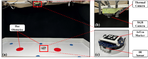
Figure 10: The experiment setup: (a) experimental platform; (b) cameras; (c) Mona robot.

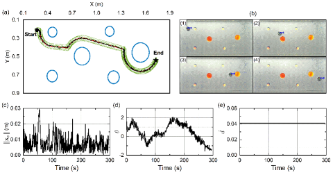
Figure 11: The experimental scenario with six obstacles: (a) the generated path (red line) and the actual trajectory (black line) of the WMR; (b) screenshots of the experiment; (c) position error; (d) WMR’s orientation; (e) parameter estimation $\hat{d}$.

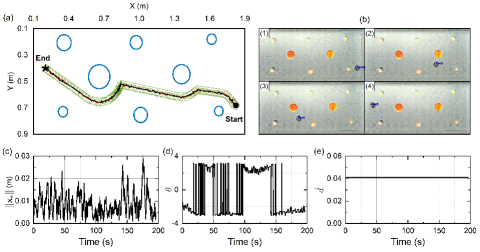
Figure 12: The experimental scenario with eight obstacles: (a) the generated path (red line) and the actual trajectory (black line) of the WMR; (b) screenshots of the experiment; (c) position error; (d) WMR’s orientation; (e) parameter estimation $\hat{d}$.

VI Conclusion

In this paper, we have proposed an integrated path planning and tube-following control scheme for collision-free navigation of WMRs in a convex workspace cluttered with multiple spherical obstacles. A path planner was designed using Bouligand’s tangent cones to generate safe, collision-free motion paths for the WMR. The resulting vector field asymptotically guides the WMR from almost all initial configurations in the free space towards the goal location, without colliding with any obstacles along the way. Then, an adaptive tube-following controller was derived, which guarantees that the actual trajectory of the WMR remains within a predefined safe tube around the reference trajectory, despite the presence of disturbances. The tube-following control significantly enhances the safety of robot navigation in the perturbed scenarios. In particular, the proposed closed-loop navigation strategy can be implemented using only the local sensing information. Finally, numerical simulations and experiments illustrate the effectiveness of the proposed autonomous navigation algorithm. Future work will focus on reactive collision-free navigation of multiple WMRs.

[Proof of Theorem 2]

From (18) and (19), it follows that $\bm{\tau}(\mathbf{x})\in\mathbf{T}_{\mathcal{X}_{\epsilon}}(\mathbf{x})$ for all $\mathbf{x}\in\mathcal{X}_{\epsilon}$, which according to Theorem 1 suggests that the free space $\mathcal{X}_{\epsilon}$ is forward invariant.

As previously stated, $\bm{\tau}(\mathbf{x})$ is piecewise continuously differentiable, indicating that it is locally Lipschitz on its domain $\mathcal{X}$ [32]. Moreover, the free space $\mathcal{X}{\epsilon}$, as a compact subset of $\mathcal{X}$, is forward invariant. Then, it follows from [33, Theorem 3.3] that the closed-loop kinematics (11) with $\mathbf{x}(0)\in\mathcal{X}_{\epsilon}$ has a unique solution that is defined for all $t\geq 0$. Subsequently, we show that the unique solution converges to a set of stationary points. To this end, we consider the following LFC:

$$W(\mathbf{x})=\dfrac{1}{2}\|\mathbf{x}-\mathbf{x}^{\ast}\|^{2}.$$ (49)

For ease of analysis, (18) is rewritten as

$$\bm{\tau}(\mathbf{x})=\underbrace{(c(\mathbf{x})\mathbf{I}_{2}+(1-c(\mathbf{x}))\mathbf{\Pi}(\mathbf{x}))}_{\mathbf{\Theta}(\mathbf{x})}\bm{\kappa}_{0}(\mathbf{x}),$$ (50)

with

$$c(\mathbf{x}):=\left\{\begin{split}&1,&\text{if}~{}&\text{d}_{\mathcal{O}}(\mathbf{x})>\epsilon^{\ast}~{}\text{or}\\ &&&\text{d}_{\mathcal{O}}(\mathbf{x})\leq\epsilon^{\ast}~{}\text{and}~{}\bm{\kappa}_{0}^{\top}(\mathbf{x})\mathbf{b}(\mathbf{x})\leq 0,\\ &0,&\text{if}~{}&\text{d}_{\mathcal{O}}(\mathbf{x})\leq\epsilon^{\ast}~{}\text{and}~{}\bm{\kappa}_{0}^{\top}(\mathbf{x})\mathbf{b}(\mathbf{x})>0.\end{split}\right.$$ (51)

Taking the time derivative of $W(\mathbf{x})$ along (11) and noting (13) and (50), one gets

$$\dot{W}(\mathbf{x})=-k_{0}(\mathbf{x})(\mathbf{x}-\mathbf{x}^{\ast})^{\top}\mathbf{\Theta}(\mathbf{x})(\mathbf{x}-\mathbf{x}^{\ast}).$$ (52)

Since $k_{0}(\mathbf{x})>0$ and $\mathbf{\Pi}(\mathbf{x})$ is positive semidefinite, one has

$$\dot{W}(\mathbf{x})\leq 0,~{}\forall\mathbf{x}\in\mathcal{X}_{\epsilon},$$ (53)

indicating that $\mathbf{x}=\mathbf{x}^{\ast}$ is a stable equilibrium of (11). From LaSalle’s invariance principle, it follows that the solution of (11) asymptotically converges to the set $\{\mathbf{x}\in\mathcal{X}_{\epsilon}\mid\dot{W}(\mathbf{x})=0\}$, i.e., a set of stationary points. One can infer from (19) and (52) that the stationary points correspond to either $\mathbf{x}=\mathbf{x}^{\ast}$ or the points satisfying $\text{d}_{\mathcal{O}}(\mathbf{x})=\epsilon$ and $\bm{\kappa}_{0}^{\top}(\mathbf{x})\mathbf{b}(\mathbf{x})/\|\bm{\kappa}_{0}(\mathbf{x})\|=1$. Therefore, for any $\mathbf{x}(0)\in\mathcal{X}_{\epsilon}$, the solution of (11) converges to the set $\{\mathbf{x}^{\ast}\}\cup_{i=1}^{n}\mathcal{S}_{i}$. The set contains $n+1$ stationary points, all of which are isolated due to Assumption 2. Geometrically, the undesired stationary point $\mathbf{s}_{i}\in\mathcal{S}_{i}$ (on the boundary of $\mathcal{O}_{i}^{\epsilon}$) and $\mathbf{x}^{\ast}$ are collinear with $\mathbf{c}_{i}$, but located on the opposite sides of $\mathbf{c}_{i}$, as seen in Fig. 13. As per (52), the analytical form of $\mathbf{s}_{i}$ is obtained as follows:

$$\mathbf{s}_{i}=(1+\alpha_{i})\mathbf{c}_{i}-\alpha_{i}\mathbf{x}^{\ast},$$ (54)

with $\alpha_{i}:=(r+r_{i}+\epsilon)\|\mathbf{x}^{\ast}-\mathbf{c}_{i}\|^{-1}$.

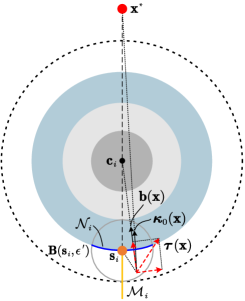
Figure 13: Illustration of the undesired stationary point $\mathbf{s}_{i}$.

The isolated stationary points $\mathbf{s}_{i}$, $i\in\mathbb{I}$ may prevent us from achieving the objective (motion-to-goal). To check the stability of $\mathbf{s}_{i}$, we define a small neighborhood of $\mathbf{s}_{i}$, i.e., an open ball $\mathcal{B}(\mathbf{s}_{i},\epsilon^{\prime})$ with $0<\epsilon^{\prime}\leq\min\{\epsilon,\epsilon^{\ast}-\epsilon\}$, such that $\bf{\kappa}_{0}^{\top}(\mathbf{x})\mathbf{b}(\mathbf{x})>0$ holds for all $\mathbf{x}\in\mathcal{B}(\mathbf{s}_{i},\epsilon^{\prime})$. When restricted on $\mathcal{B}(\mathbf{s}_{i},\epsilon^{\prime})$, the feasible set of initial configurations is $\mathcal{F}_{i}:=\mathcal{X}_{\epsilon}\cap\mathcal{B}(\mathbf{s}_{i},\epsilon^{\prime})$, and $\mathbf{x}$ evolves according to

$$\dot{\mathbf{x}}=-k_{0}(\mathbf{x})(\mathbf{I}_{2}-\phi(\text{d}_{\mathcal{O}}(\mathbf{x}))\mathbf{b}(\mathbf{x})\mathbf{b}^{\top}(\mathbf{x}))(\mathbf{x}-\mathbf{x}^{\ast}).$$ (55)

Further define two sets

$$\mathcal{M}_{i}:= ~{}\left\{\mathbf{x}\in\mathcal{X}_{\epsilon}\bigg{|}\text{d}_{\mathcal{O}_{i}}(\mathbf{x})\geq\epsilon,~{}\dfrac{\bm{\kappa}_{0}^{\top}(\mathbf{x})\mathbf{b}(\mathbf{x})}{\|\bm{\kappa}_{0}(\mathbf{x})\|}=1\right\},$$ (56)

$$\mathcal{N}_{i}:= ~{}\partial\mathcal{X}_{\epsilon}\cap\mathcal{B}(\mathbf{s}_{i},\epsilon^{\prime}).$$ (57)

Geometrically speaking, all elements of $\mathcal{M}_{i}$ form a radial line extending outward from the stationary point $\mathbf{s}_{i}$ along $\mathbf{s}_{i}-\mathbf{c}_{i}$ (see the yellow line in Fig. 13), while all elements of $\mathcal{N}_{i}$ form a curve, which is a portion of the boundary $\partial\mathcal{O}_{i}^{\epsilon}$ (see the blue curve in Fig. 13). In the following, three cases are considered: 1) $\mathbf{x}(0)\in\mathcal{B}(\mathbf{s}_{i},\epsilon^{\prime})\cap\mathcal{M}_{i}$; 2) $\mathbf{x}(0)\in\mathcal{N}_{i}\setminus\{\mathbf{s}_{i}\}$; and 3) $\mathbf{x}(0)\in\mathcal{F}_{i}\setminus(\mathcal{M}_{i}\cup\mathcal{N}_{i})$.

Case 1): $\mathbf{x}(0)\in\mathcal{B}(\mathbf{s}_{i},\epsilon^{\prime})\cap\mathcal{M}_{i}$. Note that for all $\mathbf{x}\in\mathcal{M}_{i}$, $\bm{\kappa}_{0}^{\top}(\mathbf{x})\mathbf{b}(\mathbf{x})/\|\bm{\kappa}_{0}(\mathbf{x})\|=1$ holds, whereby (55) reduces to

$$\dot{\mathbf{x}}=-k_{0}(\mathbf{x})(1-\phi(\text{d}_{\mathcal{O}}(\mathbf{x})))(\mathbf{x}-\mathbf{x}^{\ast}).$$ (58)

From (20) and (56), it is evident that $0\leq\phi(\text{d}_{\mathcal{O}}(\mathbf{x}))\leq 1$ on the set $\mathcal{M}_{i}$ and $\phi(\text{d}_{\mathcal{O}}(\mathbf{x}))=1$ only when $\mathbf{x}=\mathbf{s}_{i}$. Moreover, $k_{0}(\mathbf{x})$ is strictly larger than $0$ by construction. Hence, for all $\mathbf{x}\in\mathcal{M}_{i}\setminus\{\mathbf{s}_{i}\}$, the control vector $\bm{\tau}(\mathbf{x})$ (i.e., the right-hand side of (58)) points directly towards $\mathbf{s}_{i}$ and becomes zero when $\mathbf{x}=\mathbf{s}_{i}$, indicating that the set $\mathcal{M}_{i}$ is forward invariant. Consider the following LFC:

$$W_{i}(\mathbf{x})=\dfrac{1}{2}\|\mathbf{x}-\mathbf{s}_{i}\|^{2}.$$ (59)

The time derivative of $W_{i}(\mathbf{x})$ along (58) is given by

$$\dot{W}_{i}(\mathbf{x})=-k_{0}(\mathbf{x})(1-\phi(\text{d}_{\mathcal{O}}(\mathbf{x})))(\mathbf{x}-\mathbf{s}_{i})^{\top}(\mathbf{x}-\mathbf{x}^{\ast}).$$ (60)

Since $(\mathbf{x}-\mathbf{s}_{i})^{\top}(\mathbf{x}-\mathbf{x}^{\ast})\geq 0$ for all $\mathbf{x}\in\mathcal{M}_{i}$, one can conclude from (60) that $\dot{W}_{i}(\mathbf{x})\leq 0$ on the set $\mathcal{M}_{i}$ and $\dot{W}_{i}(\mathbf{x})=0$ only occurs at $\mathbf{x}=\mathbf{s}_{i}$. This implies that $\mathcal{M}_{i}$ is a stable manifold of $\mathbf{s}_{i}$ and any initial state on it will converge to $\mathbf{s}_{i}$. Thus, all $\mathbf{x}(0)\in\mathcal{B}(\mathbf{s}_{i},\epsilon^{\prime})\cap\mathcal{M}_{i}\subset\mathcal{M}_{i}$ will converge to $\mathbf{s}_{i}$.

Case 2): $\mathbf{x}(0)\in\mathcal{N}_{i}\setminus\{\mathbf{s}_{i}\}$. For all $\mathbf{x}\in\mathcal{N}_{i}\setminus\{\mathbf{s}_{i}\}$, we have $\text{d}_{\mathcal{O}}(\mathbf{x})=\epsilon$ and $\phi(\text{d}_{\mathcal{O}}(\mathbf{x}))=1$. As such, (55) becomes

$$\dot{\mathbf{x}}=-k_{0}(\mathbf{x})\mathbf{Q}(\mathbf{b}(\mathbf{x}))(\mathbf{x}-\mathbf{x}^{\ast}),$$ (61)

where $\mathbf{Q}(\mathbf{b}(\mathbf{x})):=\mathbf{I}_{2}-\mathbf{b}(\mathbf{x})\mathbf{b}^{\top}(\mathbf{x})$ is defined for notational brevity. Consider again the LFC $W_{i}(\mathbf{x})$ in (59). Then, taking the time derivative of $W_{i}$ along (61) and noting (54) and the fact that $(\mathbf{x}-\mathbf{c}_{i})^{\top}\mathbf{Q}(\mathbf{b}(\mathbf{x}))=0$, we get

$$\dot{W}_{i}(\mathbf{x})= ~{}k_{0}(\mathbf{x})\alpha_{i}(\mathbf{x}-\mathbf{x}^{\ast})^{\top}\mathbf{Q}(\mathbf{b}(\mathbf{x}))(\mathbf{x}-\mathbf{x}^{\ast})$$

$$-k_{0}(\mathbf{x})(1-\alpha_{i})(\mathbf{x}-\mathbf{c}_{i})^{\top}\mathbf{Q}(\mathbf{b}(\mathbf{x}))(\mathbf{x}-\mathbf{x}^{\ast})$$

$$= ~{}k_{0}(\mathbf{x})\alpha_{i}(\mathbf{x}-\mathbf{x}^{\ast})^{\top}\mathbf{Q}(\mathbf{b}(\mathbf{x}))(\mathbf{x}-\mathbf{x}^{\ast})$$

$$= ~{}k_{0}(\mathbf{x})\alpha_{i}(1-\cos\psi)\|\mathbf{x}-\mathbf{x}^{\ast}\|^{2}>0,$$ (62)

where $\psi$ is the angle between the vectors $\mathbf{b}(\mathbf{x})$ and $\bm{\kappa}_{0}(\mathbf{x})$ and satisfies $0<\psi<\pi/2$ for all $\mathbf{x}\in\mathcal{N}_{i}\setminus\{\mathbf{s}_{i}\}$. Further consider the following LFC:

$$V_{i}(\mathbf{x})=\frac{1}{2}\|\mathbf{x}-\mathbf{c}_{i}\|^{2},$$ (63)

whose time derivative along (61) is given by

$$\dot{V}_{i}(\mathbf{x})=-k_{0}(\mathbf{x})(\mathbf{x}-\mathbf{c}_{i})^{\top}\mathbf{Q}(\mathbf{b}(\mathbf{x}))(\mathbf{x}-\mathbf{x}^{\ast})=0,$$ (64)

showing that for all $\mathbf{x}\in\mathcal{N}_{i}\setminus\{\mathbf{s}_{i}\}$, the control vector is tangent to the boundary of $\mathcal{O}_{i}^{\epsilon}$, thus directing the robot to move along $\partial\mathcal{O}_{i}^{\epsilon}$. In view of (VI) and (64), we can conclude that if $\mathbf{x}(0)\in\mathcal{N}_{i}\setminus{\mathbf{s}_{i}}$, then $\mathbf{x}$ will keep away from $\mathbf{s}_{i}$ along $\partial\mathcal{O}_{i}^{\epsilon}$ until it leaves the set $\mathcal{B}(\mathbf{s}_{i},\epsilon^{\prime})$.

Case 3): $\mathbf{x}(0)\in\mathcal{F}_{i}\setminus(\mathcal{M}_{i}\cup\mathcal{N}_{i})$. Actually, for any $\mathbf{x}\in\mathcal{F}_{i}\setminus(\mathcal{M}_{i}\cup\mathcal{N}_{i})$, it holds that $\phi(\text{d}_{\mathcal{O}}(\mathbf{x}))\in(0,1)$, and $\bf{\kappa}_{0}(\mathbf{x})$ and $\mathbf{b}(\mathbf{x})$ are not collinear. Moreover, we can decompose $\bm{\tau}(\mathbf{x})=\mathbf{\Pi}(\mathbf{x})\bm{\kappa}{0}(\mathbf{x})$ into two components: the component $\bm{\tau}(\mathbf{x})_{\parallel}=\mathbf{b}(\mathbf{x})\mathbf{b}^{\top}(\mathbf{x})\bm{\tau}(\mathbf{x})$ parallel to $\mathbf{b}(\mathbf{x})$ and the component $\bm{\tau}(\mathbf{x})_{\perp}=(\mathbf{I}_{2}-\mathbf{b}(\mathbf{x})\mathbf{b}^{\top}(\mathbf{x}))\bm{\tau}(\mathbf{x})$ perpendicular to $\mathbf{b}(\mathbf{x})$, as shown in Fig. 13. With (19) in mind, one can verify that

$$\mathbf{b}^{\top}(\mathbf{x})\bm{\tau}(\mathbf{x})_{\parallel}= ~{}\mathbf{b}^{\top}(\mathbf{x})\bm{\tau}(\mathbf{x})$$

$$= ~{}(1-\phi(\text{d}_{\mathcal{O}}(\mathbf{x})))\mathbf{b}^{\top}(\mathbf{x})\bm{\kappa}_{0}(\mathbf{x})>0,$$ (65)

which implies that $\bm{\tau}(\mathbf{x}){\parallel}$ and the bearing vector $\mathbf{b}(\mathbf{x})$ have the same direction, causing $\bm{\tau}(\mathbf{x}){\parallel}$ to point towards $\mathbf{c}_{i}$. A straightforward calculation yields $(\mathbf{I}_{2}-\mathbf{b}(\mathbf{x})\mathbf{b}^{\top}(\mathbf{x})\mathbf{\Pi}(\mathbf{x})=\mathbf{Q}(\mathbf{b}(\mathbf{x}))$, which allows us to express $\bm{\tau}(\mathbf{x})_{\perp}=\mathbf{Q}(\mathbf{b}(\mathbf{x}))\bm{\kappa}_{0}(\mathbf{x})$. Under $\bm{\tau}(\mathbf{x})_{\perp}$, (55) turns to be (61), which results in $\dot{W}_{i}(\mathbf{x})>0$ as seen in (VI). Thus, $\bm{\tau}(\mathbf{x})_{\perp}$ generates a velocity component tangent to $\mathbf{b}$, causing $\mathbf{x}$ to move away from $\mathbf{s}_{i}$. Since $\bm{\tau}(\mathbf{x})$ and the vector $\mathbf{s}_{i}-\mathbf{x}$ are situated on opposite sides of $\mathbf{b}(\mathbf{x})$ (see Fig. 13), $\mathbf{x}$ cannot move toward $\mathbf{s}_{i}$ on the set $\mathcal{F}_{i}\setminus(\mathcal{M}_{i}\cup\mathcal{N}_{i})$. From Fig. 13, one can intuitively observe that $\bm{\tau}(\mathbf{x})$ guides $\mathbf{x}$ towards the boundary of $\mathcal{O}_{i}^{\epsilon}$ (attributed to $\bm{\tau}(\mathbf{x})_{\parallel})$, while simultaneously keeping away from the manifold $\mathcal{M}_{i}$ (attributed to $\bm{\tau}(\mathbf{x})_{\perp}$). Therefore, for any $\mathbf{x}(0)\in\mathcal{F}_{i}\setminus(\mathcal{M}_{i}\cup\mathcal{N}_{i})$, the solution of (11) will either directly leaves the ball $\mathcal{B}(\mathbf{s}_{i},\epsilon^{\prime})$, or first converges to the set $\mathcal{N}_{i}\setminus\{\mathbf{s}_{i}\}$ and then leaves the ball $\mathcal{B}(\mathbf{s}_{i},\epsilon^{\prime})$ along $\partial\mathcal{O}_{i}^{\epsilon}$ (as shown in Case 2).

The three cases above demonstrate that each stationary point $\mathbf{s}_{i}$ ($i\in\mathbb{I}$) is an unstable fixed point, but there exists one line of initial conditions, namely the stable manifold $\mathcal{M}_{i}$, that is attracted to $\mathbf{s}_{i}$. Note that $\mathcal{M}_{i}$ is a 1-dimensional manifold with boundary and thus has zero measure [34]. As such, $\mathbf{x}^{\ast}$ is an almost globally asymptotically stable equilibrium, with a basin of attraction consisting of the free space $\mathcal{X}_{\epsilon}$, except for a set of measure zero. Furthermore, as $\mathbf{x}^{\ast}\in\text{int}(\mathcal{X}_{\epsilon})$, there certainly exists $r^{\ast}>0$ such that $\text{d}_{\mathcal{O}}(\mathbf{x})>\epsilon^{\ast}$ for all $\mathbf{x}\in\mathcal{B}(\mathbf{x}^{\ast},r^{\ast})$. On the ball $\mathcal{B}(\mathbf{x}^{\ast},r^{\ast})$, the kinematics reduces to

$$\dot{\mathbf{x}}=-k_{0}(\mathbf{x})(\mathbf{x}-\mathbf{x}^{\ast}),$$ (66)

It can be easily verified that $k_{0}(\mathbf{x})\geq\alpha/\sqrt{(r^{\ast})^{2}+\beta^{2}}$ on the ball $\mathcal{B}(\mathbf{x}^{\ast},r^{\ast})$. Given this, (66) implies the local exponential stability of $\mathbf{x}=\mathbf{x}^{\ast}$. Furthermore, by using the inequality $|z|-z^{2}/\sqrt{z^{2}+\beta^{2}}\leq\beta$, $\forall z\in\mathbb{R}$, (52) reduces to

$$\dot{W}_{i}(\mathbf{x})\leq -\alpha\|\mathbf{x}-\mathbf{x}^{\ast}\|+\alpha\beta$$

$$\leq -\sqrt{2}\alpha W_{i}(\mathbf{x})^{\frac{1}{2}}+\alpha\beta,$$ (67)

which warrants the locally practical finite-time convergence of $\mathbf{x}=\mathbf{x}^{\ast}$ [35, Lemma 3.6]. This completes the proof. $\hfill\Box$

References

- [1] G. Klancar, A. Zdesar, S. Blazic, and I. Skrjanc, Wheeled mobile robotics: from fundamentals towards autonomous systems. Butterworth-Heinemann, 2017.
- [2] X. Chu, R. Ng, H. Wang, and K. W. S. Au, “Feedback control for collision-free nonholonomic vehicle navigation on SE (2) with null space circumvention,” IEEE/ASME Transactions on Mechatronics, vol. 27, no. 6, pp. 5594–5604, 2022.
- [3] V. J. Lumelsky, Sensing, intelligence, motion: how robots and humans move in an unstructured world. John Wiley & Sons, 2005.
- [4] S. Berkane, “Navigation in unknown environments using safety velocity cones,” in 2021 American Control Conference (ACC). IEEE, 2021, pp. 2336–2341.
- [5] O. Khatib, “Real-time obstacle avoidance for manipulators and mobile robots,” The International Journal of Robotics Research, vol. 5, no. 1, pp. 90–98, 1986.
- [6] J.-O. Kim and P. Khosla, “Real-time obstacle avoidance using harmonic potential functions,” IEEE Transactions on Robotics and Automation, vol. 8, no. 3, pp. 338–349, 1992.
- [7] L. Valbuena and H. G. Tanner, “Hybrid potential field based control of differential drive mobile robots,” Journal of Intelligent & Robotic Systems, vol. 68, pp. 307–322, 2012.
- [8] H. Li, W. Liu, C. Yang, W. Wang, T. Qie, and C. Xiang, “An optimization-based path planning approach for autonomous vehicles using the dynefwa-artificial potential field,” IEEE Transactions on Intelligent Vehicles, vol. 7, no. 2, pp. 263–272, 2021.
- [9] E. Rimon and D. Koditschek, “Exact robot navigation using artificial potential functions,” IEEE Transactions on Robotics and Automation, vol. 8, no. 5, pp. 501–518, 1992.
- [10] C. Wang, L. Wang, J. Qin, Z. Wu, L. Duan, Z. Li, M. Cao, X. Ou, X. Su, W. Li et al., “Path planning of automated guided vehicles based on improved a-star algorithm,” in 2015 IEEE International Conference on Information and Automation. IEEE, 2015, pp. 2071–2076.
- [11] S. Erke, D. Bin, N. Yiming, Z. Qi, X. Liang, and Z. Dawei, “An improved a-star based path planning algorithm for autonomous land vehicles,” International Journal of Advanced Robotic Systems, vol. 17, no. 5, p. 1729881420962263, 2020.
- [12] I. Noreen, A. Khan, and Z. Habib, “Optimal path planning using rrt* based approaches: a survey and future directions,” International Journal of Advanced Computer Science and Applications, vol. 7, no. 11, 2016.
- [13] J. Tu and S. X. Yang, “Genetic algorithm based path planning for a mobile robot,” in 2003 IEEE International Conference on Robotics and Automation (Cat. No. 03CH37422), vol. 1. IEEE, 2003, pp. 1221–1226.
- [14] M. M. Costa and M. F. Silva, “A survey on path planning algorithms for mobile robots,” in 2019 IEEE International Conference on Autonomous Robot Systems and Competitions (ICARSC). IEEE, 2019, pp. 1–7.
- [15] Y. Yan, L. Peng, J. Wang, H. Zhang, T. Shen, and G. Yin, “A hierarchical motion planning system for driving in changing environments: Framework, algorithms, and verifications,” IEEE/ASME Transactions on Mechatronics, 2022.
- [16] V. J. Lumelsky and T. Skewis, “Incorporating range sensing in the robot navigation function,” IEEE transactions on Systems, Man, and Cybernetics, vol. 20, no. 5, pp. 1058–1069, 1990.
- [17] K. N. McGuire, G. C. de Croon, and K. Tuyls, “A comparative study of bug algorithms for robot navigation,” Robotics and Autonomous Systems, vol. 121, p. 103261, 2019.
- [18] G. Lionis, X. Papageorgiou, and K. J. Kyriakopoulos, “Locally computable navigation functions for sphere worlds,” in Proceedings 2007 IEEE International Conference on Robotics and Automation. IEEE, 2007, pp. 1998–2003.
- [19] I. Filippidis and K. J. Kyriakopoulos, “Adjustable navigation functions for unknown sphere worlds,” in 2011 50th IEEE Conference on Decision and Control and European Control Conference. IEEE, 2011, pp. 4276–4281.
- [20] S. Paternain and A. Ribeiro, “Stochastic artificial potentials for online safe navigation,” IEEE Transactions on Automatic Control, vol. 65, no. 5, pp. 1985–2000, 2019.
- [21] O. Arslan and D. E. Koditschek, “Sensor-based reactive navigation in unknown convex sphere worlds,” The International Journal of Robotics Research, vol. 38, no. 2-3, pp. 196–223, 2019.
- [22] L. Huber, A. Billard, and J.-J. Slotine, “Avoidance of convex and concave obstacles with convergence ensured through contraction,” IEEE Robotics and Automation Letters, vol. 4, no. 2, pp. 1462–1469, 2019.
- [23] Y. Zhu, Z. Wang, C. Chen, and D. Dong, “Rule-based reinforcement learning for efficient robot navigation with space reduction,” IEEE/ASME Transactions on Mechatronics, vol. 27, no. 2, pp. 846–857, 2021.
- [24] H. M. Becerra, J. A. Colunga, and J. G. Romero, “Simultaneous convergence of position and orientation of wheeled mobile robots using trajectory planning and robust controllers,” International Journal of Advanced Robotic Systems, vol. 15, no. 1, p. 1729881418754574, 2018.
- [25] X. Liang, H. Wang, Y.-H. Liu, Z. Liu, and W. Chen, “Leader-following formation control of nonholonomic mobile robots with velocity observers,” IEEE/ASME Transactions on Mechatronics, vol. 25, no. 4, pp. 1747–1755, 2020.
- [26] G. Bouligand, “Introduction à la géométrie infinitésimale directe,” (No Title), 1932.
- [27] M. Nagumo, “Über die lage der integralkurven gewöhnlicher differentialgleichungen,” Proceedings of the Physico-Mathematical Society of Japan. 3rd Series, vol. 24, pp. 551–559, 1942.
- [28] J. M. Lee, Manifolds and Differential Geometry. American Mathematical Society, 2022, vol. 107.
- [29] H. K. Khalil, “Adaptive output feedback control of nonlinear systems represented by input-output models,” IEEE transactions on Automatic Control, vol. 41, no. 2, pp. 177–188, 1996.
- [30] S. S. Ge and Y. J. Cui, “New potential functions for mobile robot path planning,” IEEE Transactions on Robotics and Automation, vol. 16, no. 5, pp. 615–620, 2000.
- [31] F. Arvin, J. Espinosa, B. Bird, A. West, S. Watson, and B. Lennox, “Mona: an affordable open-source mobile robot for education and research,” Journal of Intelligent & Robotic Systems, vol. 94, pp. 761–775, 2019.
- [32] R. W. Chaney, “Piecewise functions in nonsmooth analysis,” Nonlinear Analysis: Theory, Methods & Applications, vol. 15, no. 7, pp. 649–660, 1990.
- [33] H. K. Khalil, Nonlinear Systems (3rd edn). NJ: Prentice Hall, 2002.
- [34] J. W. Milnor and D. W. Weaver, Topology from the differentiable viewpoint. Princeton University Press, 1997.
- [35] Z. Zhu, Y. Xia, and M. Fu, “Attitude stabilization of rigid spacecraft with finite-time convergence,” International Journal of Robust and Nonlinear Control, vol. 21, no. 6, pp. 686–702, 2011.